Preprint
Article

This version is not peer-reviewed.

Pore Structure Analysis of Growing Media Using X-Ray Microcomputed Tomography

Submitted:

30 September 2025

Posted:

30 September 2025

You are already at the latest version

Abstract

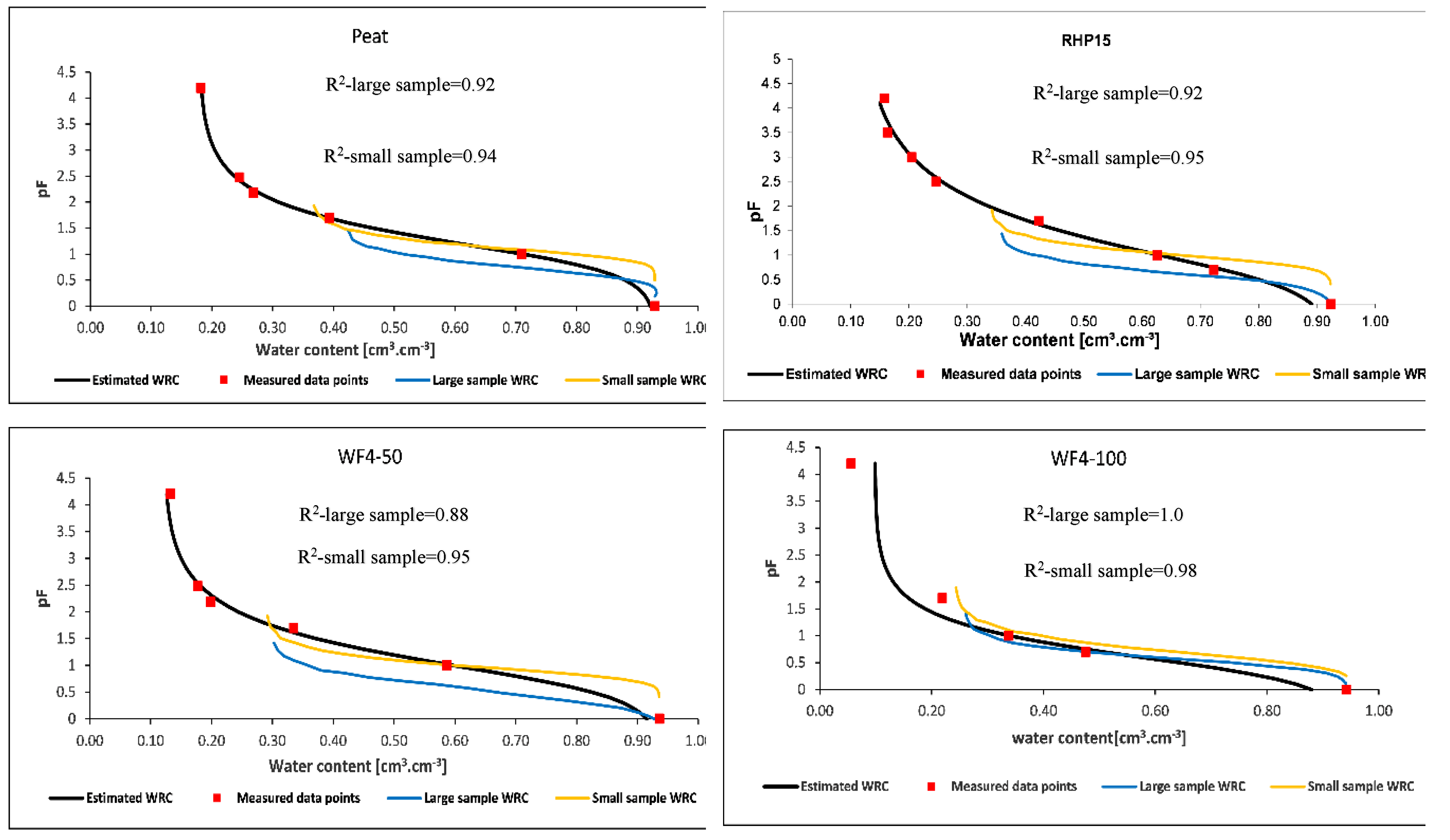
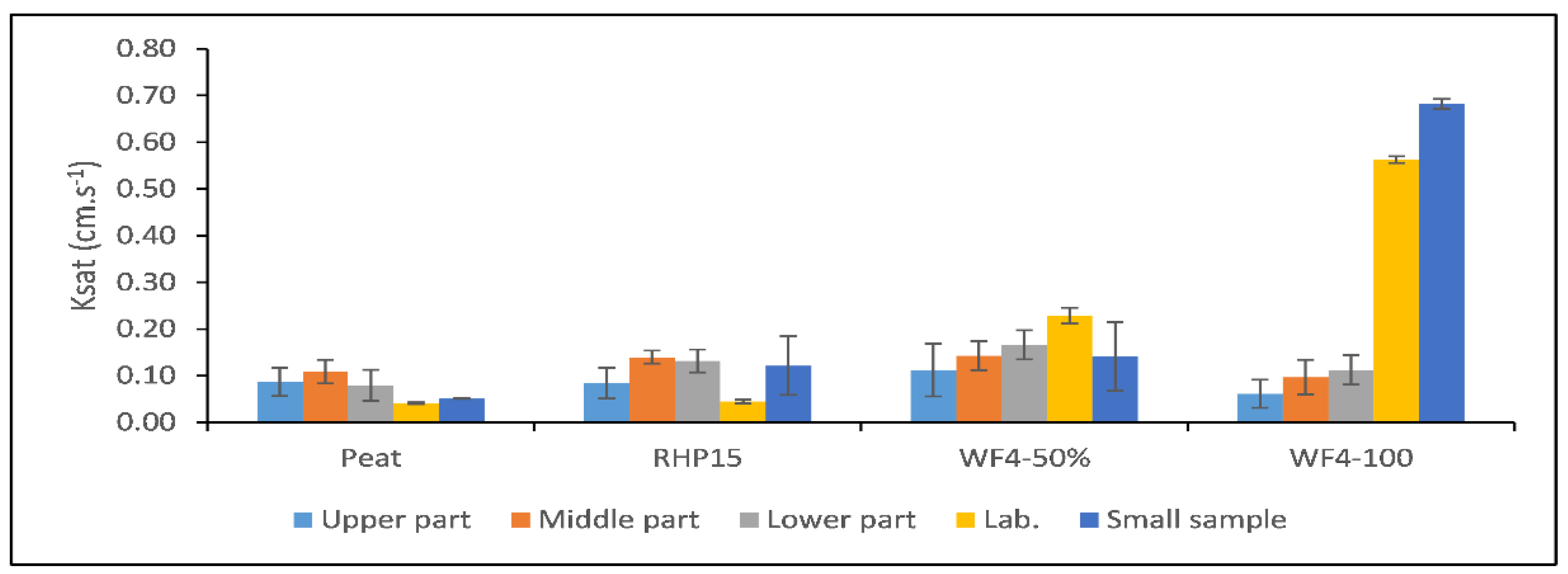
This study investigated the representative elementary volume (REV) for visible porosity in horticultural growing media (peat, commercial mixture, treated wood fibre/peat, pure wood fibre) using x-ray micro-computed tomography (µCT) with 2D and 3D image division, pore morphology, water retention curve (WRC), and saturated hydraulic conductivity (Ksat) via pore network modelling (PNM). Two sample sizes (10 x 10 cm, 3 x 3 cm, height x diameter) with resolutions of 46 and 15 µm were analysed. REV was assessed using deterministic (dREV) and statistical (sREV) criteria, evaluating porosity and coefficient of variation across subvolumes. Results showed 3D division of large samples achieved REV only for pure wood fibre (8000–10000 µm), while 2D division met both criteria for all media. For small samples, 3D division achieved REV only for wood fibre/peat mixture, but 2D division succeeded for all media above 3,000 µm. Pore analyses indicated pure wood fibre had the largest, most connected pores, enhancing drainage, while peat showed complex, retentive structures. WRCs aligned well with lab data (R2 > 0.88). PNM Ksat estimates from small images were more accurate, with discrepancies (21–172%) due to segmentation artefacts. Future studies should incorporate permeability or tortuosity and explore multiscale imaging for improved hydrophysical predictions. This study also highlights advantages unique to X-ray µCT compared to standard laboratory methods, e.g. direct three-dimensional quantification of pore structure parameters and an image-based determination of the REV.

Keywords: 
;  ;  ;  ;  

1. Introduction

The structural arrangement of porous medium components is critical to its function, and accurately measuring its internal architecture is crucial for understanding the processes that govern its development. Soil presents a challenging study due to its diverse mix of mineral particles, air- and water-filled pores, and organic matter across various scales, which has led to its characterisation as 'the most complex biomaterial on the planet’ [1,2,3]. Consequently, our understanding of how soil structure forms, stabilises, and degrades remains incomplete. Because soil is organised hierarchically in a complex and dynamic manner, progress in understanding its behaviour requires detailed spatial assessments of its constituent configurations in three dimensions (3D) and precise quantification of the underlying processes that drive changes over time.
Like mineral soil, a growing medium is a porous material. The hydro-physical properties of growing media play a critical role in determining their suitability for plant growth, water retention, and nutrient availability in agricultural and horticultural applications [2,4,5]. Among these properties, the pore structure encompassing porosity, pore size distribution, and pore connectivity stands out as a fundamental factor influencing the performance of growing media. Understanding the intricate details of pore structures is essential for optimising hydrodynamic strategies, enhancing root development, and improving overall crop productivity [6,7]. Traditional methods for analysing pore structures, such as mercury intrusion porosimetry for soils or water retention curve analysis for soils and growing media, often provide limited insights into the three-dimensional (3D) architecture of pores and may involve destructive techniques that alter the sample. In practice, the hydraulic properties of growing media are determined with analytical laboratory methods. For example, the saturated hydraulic conductivity of growing media can be determined with the standard procedure of constant head (DIN EN 19683, 1998) [8], and the water retention curve with (DIN EN 13041, 2011 and DIN EN ISO 11274, 2019) [9,10]. Recently, another laboratory centrifuge method was developed by [11], by which the water retention curve of growing media is determined. However, these laboratory procedures quantify bulk hydraulic behaviour but do not resolve 3D pore geometry and may partially alter sample structure. Beyond laboratory tests, direct simulation models have been used to determine the hydraulic properties of growing media [12,13,14]. Likewise, an inverse numerical simulation model has been used to determine the hydraulic properties and parameters of growing media [15]. These numerical approaches complement measurements but rely on simplifying assumptions about pore geometry and calibration data, and thus still do not provide spatially explicit internal structure. Taken together, these limitations highlight the need for advanced, non-destructive techniques capable of providing high-resolution, spatially resolved data on the internal structure of growing media. Accordingly, X-ray microcomputed tomography (µCT) has provided a non-destructive tool for visualising and quantifying the three-dimensional structure of porous media over the last three decades [16,17] adding valuable spatial information not available through standard laboratory tests.
µCT has emerged as a powerful tool for non-invasively characterising the 3D pore structure of porous materials, offering significant advantages over conventional methods. By generating detailed 3D images of the internal architecture of porous media, µCT enables researchers to quantify key structural parameters, such as total porosity [18], pore size distribution [19], permeability [20], water retention curve (WRC) [21] and connectivity [22], with unprecedented accuracy. These parameters are critical for understanding how soils and growing media interact with water, air, and roots, ultimately influencing plant health and yield. Furthermore, µCT allows for the repeated analysis of the same sample under varying conditions, providing insights into dynamic processes such as water infiltration, compaction, or degradation of the growing medium over time [22,23,24,25,26,27]. The µCT provides superior insights into soil pore structure by non-destructively capturing high-resolution, three-dimensional images of the internal porous media, enabling precise quantification of properties critical to hydraulic behaviour [28]. The µCT scanner operates by emitting X-rays at controlled energy levels through soil samples, detecting differential absorption based on material density [29]. This generates detailed grayscale images, where contrasts between solid soil particles and pore spaces are resolved at micrometre scales (µm/pixel resolution). Binarisation processes these images to distinguish pores from solids, necessary for quantitative analysis of pore characteristics [30]. µCT images have the potential for identifying the geometrical shapes and connectivity of the pores within the porous material, which are frequently called Minkowski functionals [3,31]. Additionally, the µCT images can provide a network of the pores and throats by which the permeability and saturated hydraulic conductivity of samples can be estimated using the pore network modelling [32,33]. The µCT technique derives porosity by calculating the volume fraction of pore spaces relative to the total sample volume, offering accurate measurements of open and closed porosity. Pore surface area is computed by tracing the interfaces between pores and solids in the 3D reconstructions, providing insights into surface interactions affecting water flow [34]. The pore size distribution is determined by analysing the size range of individual pores, revealing the prevalence of macropores, mesopores and micropores, which directly influences permeability. It may be noted, however, that µCT images can only detect pores larger than the image resolution. Therefore, only a part of the micropores can be evaluated from images. Critical pore diameter, the size of the largest interconnected pore controlling flow, is identified through connectivity analysis, highlighting pathways for water movement [35]. The water retention curve is inferred by correlating pore size distribution with capillary pressure, as smaller pores retain water more strongly [30]. Permeability and saturated hydraulic conductivity (Ksat) are estimated by modelling fluid flow through the interconnected pore network, where open pores enhance Ksat, while closed pores and finer textures reduce it. By quantifying these parameters, µCT elucidates the structural controls on soil hydraulic properties, offering a robust tool for predicting water and solute transport.
The µCT image analysis has been commonly used in the fields of mineral soils and rock reservoirs. The major characteristics of porous media, evaluated using the µCT image method, include the representative elementary volume (REV), pore structure metrics (Minkowski functionals), water retention curve (WRC), and permeability [36,37,38]. A limited number of studies have been conducted on specific growing media using µCT images. For example, Turunen et al. [39] quantified water retention, pore size distribution and sample shrinkage of Sphagnum-based growing medium and Quinton et al. [40] estimated volumetric water content of the peat-based growing medium. However, to the best of our knowledge, no comprehensive µCT image package has yet been published that evaluates all the REV, WRC, Minkowski functionals, and permeability in a unified framework in growing media with different structures. Therefore, there is a need to conduct this study to develop an integrated framework that enables the simultaneous extraction and analysis of these key parameters from µCT images, which would significantly advance the quantitative characterisation of porous growing media.
The objectives of this study were to: (1) quantify the representative elementary volume (REV) of the imaged samples; (2) evaluate the pore structure parameters (including Minkowski functionals) of the growing media; (3) derive the water retention curve (WRC) from the image data; and (4) simulate the saturated hydraulic conductivity of the imaged growing media using a pore network model (PNM).

2. Materials and Methods

2.1. Laboratory Experiment

2.1.1. The Studied Growing Media

For this research, four different types of growing media were chosen to represent a wide spectrum of particle sizes, organic matter content, and raw materials, including a peat-free substrate. These substrates used were pure white peat (Peat), a commercial mixture containing black and white sphagnum peat, perlite, compost, wood fibre and clay (RHP15), pure thermally treated wood fibre (WF4-100), and a 50% v/v mixture of the peat and wood fibre (WF4-50). Initially, the basic physical and chemical properties of these growing media were characterised (Table 1). Electrical conductivity (EC) was measured using a 1:5 ratio of substrate to distilled water, v/v, while pH was determined with a 1:2.5 ratio of substrate to 0.02 mol/L CaCl2, v/v, as per [41]. The pH values ranged from 3.2 (peat) to 5.9 (RHP15), and EC ranged from 0.05 dS m−1 (Peat) to 0.29 dS m−1 (RHP15), depending on the materials and fertilisers used. Organic matter percentages were assessed by ignition loss according to [42], varying from 65.09% mass (RHP15) to 99.40% m/m (WF4-100). Mean weighted diameters [43] spanned from very fine (1.18 mm; Peat) to coarse (4.93 mm; RHP15) (Table 1). Particle density was estimated from organic and mineral matter via ignition loss [42], while pore volume was determined from particle density and bulk density following DIN EN 13041 [9]. Furthermore, saturated hydraulic conductivity of the substrates was measured using the constant head method [8].

2.1.2. Water Retention Curve

The standard procedure for determining the WRC of growing media follows the DIN reference method [9]. In this process, two polyethylene vinyl chloride (PVC) cylinders (16 cm in height, 16 cm in diameter, holding 3.2 litres each) were filled with each substrate type without compaction. These cylinders were then placed in a water bath, where water was gradually added from the base of the cylinders to a level one centimetre below the top over 30 minutes. This bottom-up saturation method was used to minimise air entrapment within the substrate pores. The substrates remained saturated for 24 hours. Following saturation, the samples were placed on a sandbox suction table and subjected to a −50 hPa pressure head for 48 hours to reach equilibrium. Subsequently, the substrate from each cylinder was emptied onto a tray, homogenised, and then refilled into four double-ring samplers (serving as four replicates per substrate type). Each double ring consisted of an upper and lower ring, both measuring 5 cm in height and 10 cm in diameter. A non-biodegradable synthetic mesh was attached to the base of each lower ring to secure the material. The filled rings were resaturated (as above) and subsequently positioned on the sandbox, where successive pressure heads of −5, −10, and −50 hPa (corresponding to pF values of 0.7, 1.0, and 1.7) were applied with respect to the centre of the lower ring as described in [9]. After using the first pressure head (pF 0.7), the upper rings and excess material were carefully removed. The lower rings were weighed after equilibrium at each pressure step. Once the final suction at pF 1.7 was completed, the remaining material in the lower rings was dried at 105 °C for 48 hours to determine gravimetric water content and dry matter. Dry bulk density (BD) was then calculated from the dried sample’s weight and volume. To capture water retention at higher suctions, additional pressure heads of −158, −316, and −15848 hPa (equivalent to pF values of 2.2, 2.5, and 4.2) were applied using smaller rings (1 cm in height and 5 cm in diameter) in a pressure plate apparatus [10]. The water content values obtained at different suction levels were used to construct water retention curves. The water retention data were then fitted using the Van Genuchten model [44] (Equation (1)), with the saturated water content (θs) set equal to the measured pore volume. The curve fitting was performed using Microsoft Excel’s solver tool.
S e h = θ h θ r θ s θ r = 1 + α h n m                                               h < 0 θ h = θ s                                               h 0
where Se is effective saturation; θr and θs denote the residual and saturated water contents, respectively (L3·L−3); α (L−1), n (-), and m = 1-1/n (-) are empirical parameters. Finally, the expected porosity, i.e. the porosity of pores larger than the resolution size of the µCT images, was derived from the WRC. This expected porosity was used as a reference to compare with the image-based visible porosity. The coefficient of variation (R2) was implemented between the laboratory-measured WRCs and the image-based WRCs.

2.2. Image Experiment

2.2.1. Sample Packing for Scanning

The preparation of samples for µCT analysis was conducted to ensure accurate and consistent characterisation of the growing media. Based on the bulk density of the laboratory measurements, five Plexiglas cylinders were filled with each growing medium. Each cylinder had an internal diameter of 9.4 cm and a height of 10 cm, designed to provide a representative volume for analysing the structural properties of the substrates (referred to as ‘large samples’ in the following text). These cylinders were scanned using µCT at a resolution of 46 µm per pixel to capture detailed pore structures. Additionally, two smaller tubes per growing medium were prepared, each with a diameter of 3 cm and a height of 3 cm, to support complementary analyses such as higher-resolution imaging or physical testing. These smaller tubes were scanned at a higher resolution of 15 µm per pixel to enable finer visualisation of microstructural features (referred to as ‘small samples’ in the following text). All containers were filled with care to prevent compaction artefacts, preserving the natural pore structure of the substrates and ensuring reliable data for subsequent image processing and analysis.

2.2.2. X-Ray Microcomputed Tomography Scanning

The samples consisted of cylindrical specimens categorised into large and small cylinders based on their dimensions. All samples were prepared to ensure compatibility with the µCT scanner's field of view and resolution requirements. Scans were performed using a RayScan Smart µCT scanner (RayScan Technologies GmbH, Meersburg, Germany), equipped with a FINETEC FORE 230.01C TT X-ray tube and a high-resolution flat panel detector. The detector featured a size of approximately 410 mm × 410 mm, with a resolution of 4096 × 4096 pixels and a pixel pitch of 100 µm. It offered a 16-bit dynamic range and CT-grade sensitivity. The detector supported readout rates of up to 15 frames per second in binning mode, with an optical interface and adjustable gain settings to optimise image quality. Scanning parameters were tailored to the sample size to ensure optimal image resolution and contrast. For large cylinders, 720 projections were acquired over a full 360° rotation, with the X-ray tube set to 155 kV and 145 µA, and an exposure time of 499 ms per projection. For small cylinders, the same number of projections (720) was acquired over 360°, but with the X-ray tube set to 170 kV and 150 µA, maintaining the same exposure time of 499 ms. These settings were chosen to balance penetration depth and image clarity for the respective sample sizes. Image reconstruction was performed using the proprietary RayWare5-Reco software (RayScan Technologies GmbH). The reconstructed image slices were imported into VGStudioMax 2023.2 (Volume Graphics GmbH) for visualisation and then exported as RAW files for further processing and quantitative analysis in a Python program.

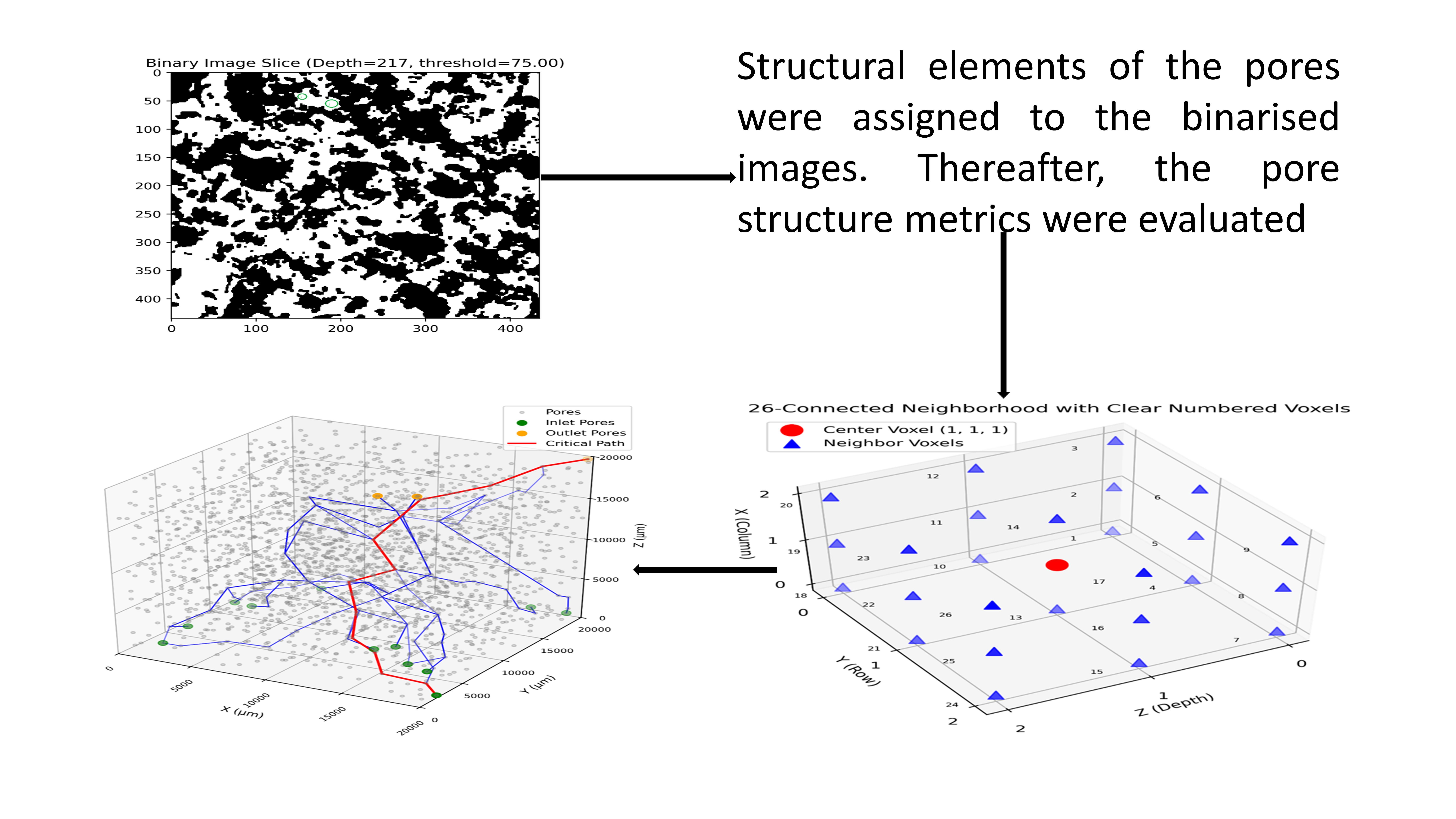
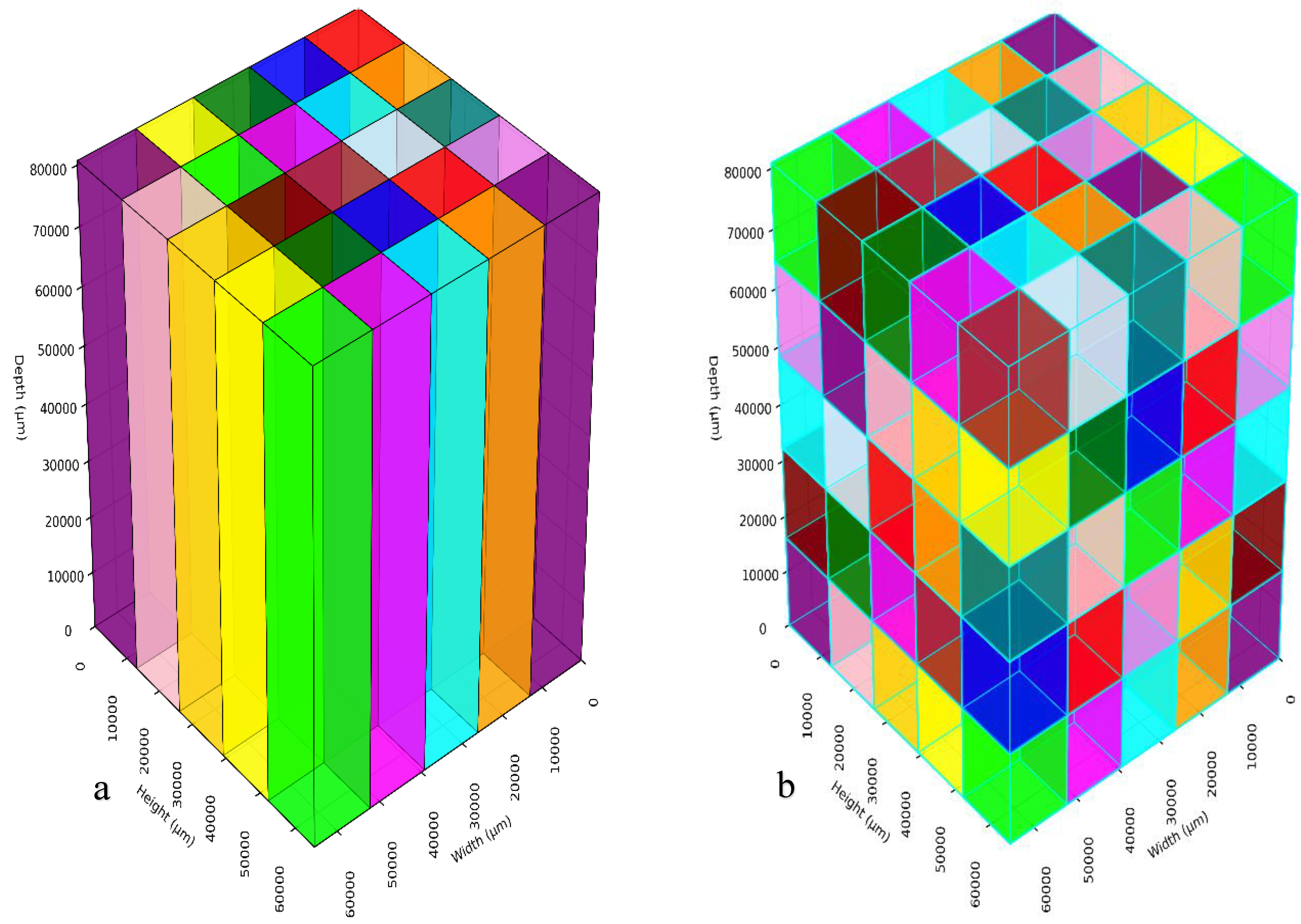
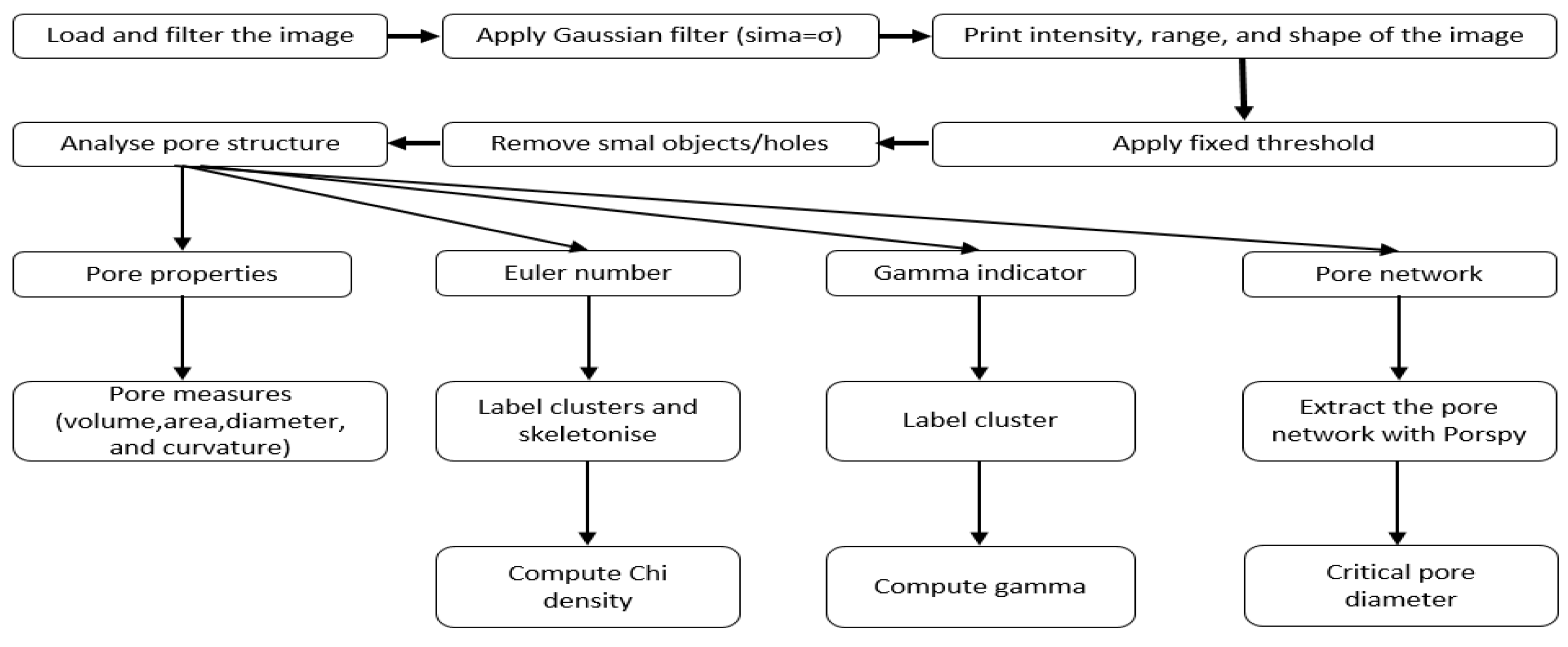
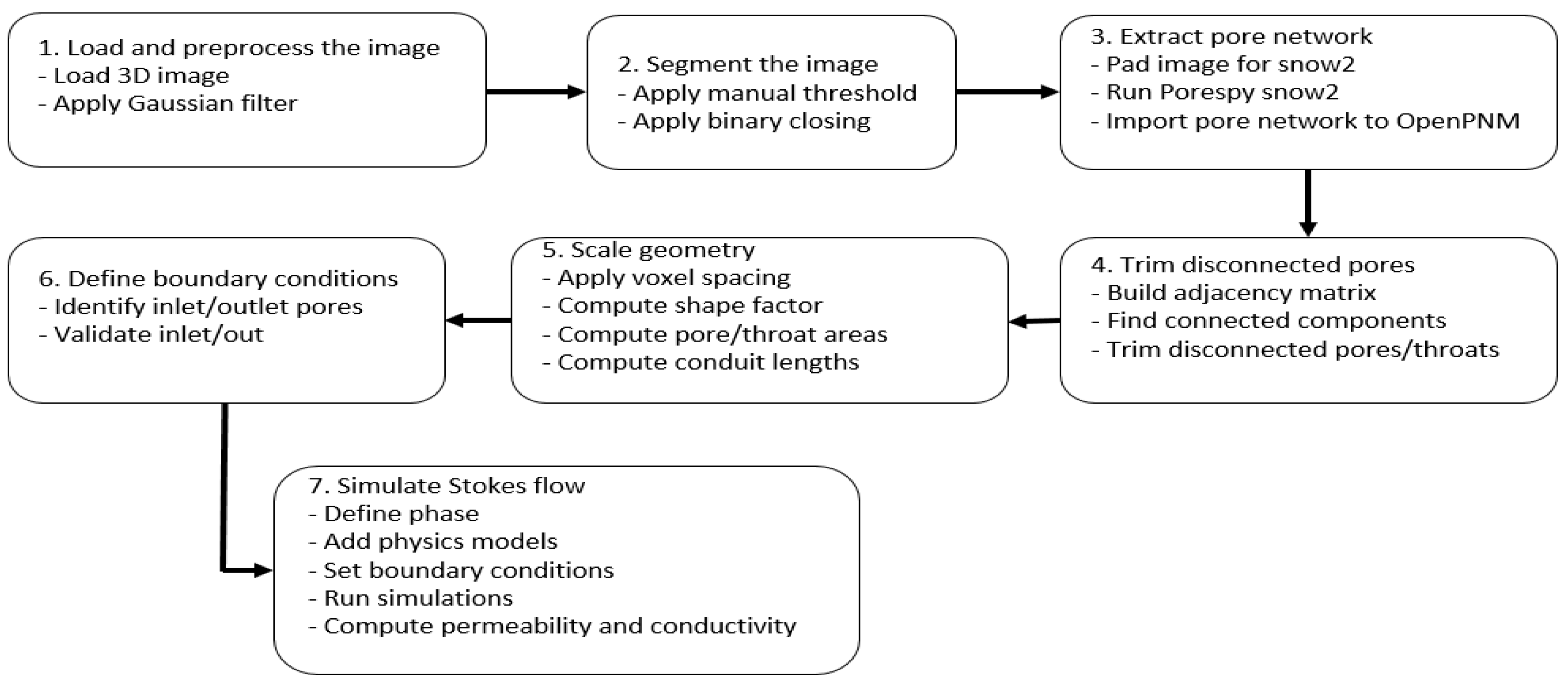
2.2.3. Image Processing and Analysis

The µCT image analysis was implemented using a combination of Python packages tailored for image processing, morphological analysis, and pore network modelling. The images were first imported with tifffile and denoised using a Gaussian filter from SciPy [45] to reduce noise. Segmentation and morphological operations, such as labelling, skeletonisation, and removal of small objects or holes, were performed using scikit-image [46]. Quantitative descriptors of pore geometry, including volume, surface area, equivalent diameter, and curvature, were derived through NumPy [47] operations and region-based measurements. Connectivity metrics such as Euler number density and the gamma indicator were computed using scikit-image and custom routines. For pore network extraction, PoreSpy’s snow2 algorithm [48] was employed to generate a network representation, which was subsequently converted into an OpenPNM [49] project to calculate network-level properties (e.g pore and throat size distributions). Visualisation of distributions was performed using matplotlib, while quantitative results and raw data arrays were stored in structured formats using pandas for further analysis. Together, these packages provided an integrated workflow from 3D image preprocessing to pore-scale structural and network analysis.
Representative Elementary Volume (REV)
The Python workflow comprised three main scripts: (i) determination of the REV based on two and three dimensional partitions, (ii) extraction of pore-structure metrics, including the WRC and Minkowski functionals, and (iii) estimation of saturated hydraulic conductivity.
For image processing, the thresholding can be global, local, or manual (visual) methods [50,51,52,53]. However, we applied a manual thresholding method to differentiate the pixel intensity of the pores from the solid particles (Table 2).
To determine the REV for each material, µCT images of the large and small samples were partitioned into two and three dimensions to assess the spatial variability of visible pore volume across different subvolume sizes (Figure 1). The large and small cubic µCT substacks used to determine the REV measured 1755, 1420, 1420 and 1601, 1250, 1250 voxels (z,y,x), resulting in a total volume of 344.5 and 8.5 cm³, respectively. The isotropic pixel sizes of 46 µm (large samples) and 15 µm (small samples), yielded single voxel volumes of 97336 µm3 and 3375 µm3, respectively. The REV procedure was identical for large and small samples; only the voxel size differed. Figure 1 shows 3D visualisations for the large samples. The analysis was performed using a Python-based workflow leveraging NumPy, SciPy, scikit-image, and Matplotlib libraries [45,46,47,54], as described below. Images were loaded using the tifffile library [55] and preprocessed with a Gaussian filter (σ = 1.0) [56] from SciPy’s ndimage module to reduce noise while maintaining structural integrity. The images were segmented using a fixed intensity threshold (manual thresholding) to distinguish pore voxels from solid voxels (Table 2), resulting in a binary image where pores were represented by 1s and solids by 0s. The visible porosity of the full volume was calculated as the fraction of pore voxels.
The volumes were then partitioned into non-overlapping cubic subvolumes by dividing each axis into n equal segments (n ϵ { 2,3,4,5,6,7,8,9,10,15,20,25,30,35,40,45, and 50}), yielding n3 subvolumes in 3D. For the 2D analysis, depth (z) was kept intact, producing n2 tiles in the (y,x) plane. The visible porosity of each subvolume was computed as the ratio of pore voxels to total voxels. For each division level n, the mean visible porosity, standard deviation, and coefficient of variation (CV, defined as the standard deviation divided by the mean) were calculated across all subvolumes; this method is referred to as statistical REV(sREV) [38,57,58,59]. The characteristic subvolume edge length was defined as the minimum of (Δz, Δy, and Δx) multiplied by the voxel size. These metrics were aggregated to assess how porosity variability changed with subvolume size. The overall mean visible porosity across all subvolumes was also computed. The REV was identified by evaluating the CV across subvolume sizes. A decreasing CV with increasing subvolume size indicates convergence toward a representative scale where porosity becomes statistically stable. The smallest subvolume size at which the CV stabilised (typically below a threshold such as 0.1) was considered the REV, ensuring that the sample’s pore structure was adequately represented for subsequent analyses. The second method for determining the REV is called a deterministic REV (dREV) [50,60,61]. Operationally, dREV was identified by locating at least three consecutive subvolumes with minimal differences in visible porosity(i.e., a locally stable plateau), providing a practical representative scale complementary to sREV.
Pore structure and WRC
A flowchart describing the image processing steps for pore structure calculations is given in Figure 2. Pore properties were quantified using the Python scikit package (scikit-image.measure). The total visible pore volume was calculated as the number of pore voxels multiplied by the voxel volume. Specific surface area was estimated by dividing the pore area by the pore volume (surface area density). The average pore diameters were derived from the equivalent sphere diameter of labelled pore regions. A distance transform (Python scipy package: scipy.ndimage.distance_transform_edt) was used to estimate pore sizes. Mean curvature density was computed from the divergence of the unit normal field derived from the distance map gradient [62,63]. Additionally, to calculate the pore size distribution, the pore volume was used to calculate the volume-equivalent sphere diameter using a standard geometrical relation [64]: D v o l u m e = 6 v π 1 3 , where v is the pore volume in µm3.
Topological properties included the Euler number density (χ), calculated as χ = N - C, where N is the number of connected pore clusters and C is the number of skeleton branches, normalised by the sample volume (mm3). The gamma indicator, γ = i = 1 N n i 2 ( i = 1 N n i ) 2 , where n i is the number of pore voxels in the i-th pore cluster and N is the total number of pore clusters, was computed to assess pore size heterogeneity [65]. The critical pore diameter was calculated as the minimum diameter along the largest inscribed sphere path that percolates from top to bottom through the pore system [66,67].
The extracted pore diameters were used to derive the matric potential using the Yang-Laplace equation [68]: |Ψ|= 2980 D , where Ψ is a matric potential in hectopascal, and D is the pore diameter in micrometres. The cumulative pore equivalent diameter was plotted versus the matric potential to draw the WRC. Note that the cumulative pore distribution reflects only µCT visible pores (resolution-limited). To reconcile with the laboratory porosity, the unresolved fraction (lab total porosity minus expected porosity) was added to the smallest diameter class.
Hydraulic conductivity calculations
A flowchart describing the image processing steps using the pore network model to calculate Ksat is shown in Figure 3.
Pore network extraction was conducted by trimming disconnected pores and throats using a custom function in the PoreSpy Python library [48], which identified the largest connected component via a connectivity matrix derived from throat connections. The structural element of (3,3,3) for the images was considered as the pores which are highly connected [69]. In this structural element, each pore is viewed as a unit cube with six faces, 12 edges, and eight vertices (26-neighbourhoods). This matrix, constructed using the compressed sparse graph module of the SciPy library, ensured only the percolating network was retained, removing isolated regions to enhance flow simulation. The extracted network was then imported into the OpenPNM Python library [49]. The pore network model function was parameterised by assigning geometric models (spherical pores and cylindrical throats) [70]. The flow modelling also incorporated the Valvatne-Blint model (equation 2), calculating throat hydraulic conductance based on pore and throat shape factors, approximating non-circular cross-sections and conduit length, where throat length was defined as the distance from the midpoint of two neighbouring pores to adjust pore resistance [71]. The Stokes flow (equation 3) model simulated fluid dynamics by solving the pressure gradient from the inlet to the outlet of the flow domain using Stokes flow algorithms. Finally, permeability was obtained from Darcy’s law (equation 4), and saturated hydraulic conductivity was derived from the permeability.
g = f π . r 2 8 μ L
where g is the hydraulic conductance, f is a shape factor calculated inside the PNP library, r is the pore radius, μ is the fluid viscosity (1.0x10⁻³) pascal per second, and L is the sample length
Q = g . p  
where Q is flow rate and Δp is the pressure difference
K = Q . L . μ A . Δ p
where K is permeability and A is the cross-sectional area.

3. Results and Discussion

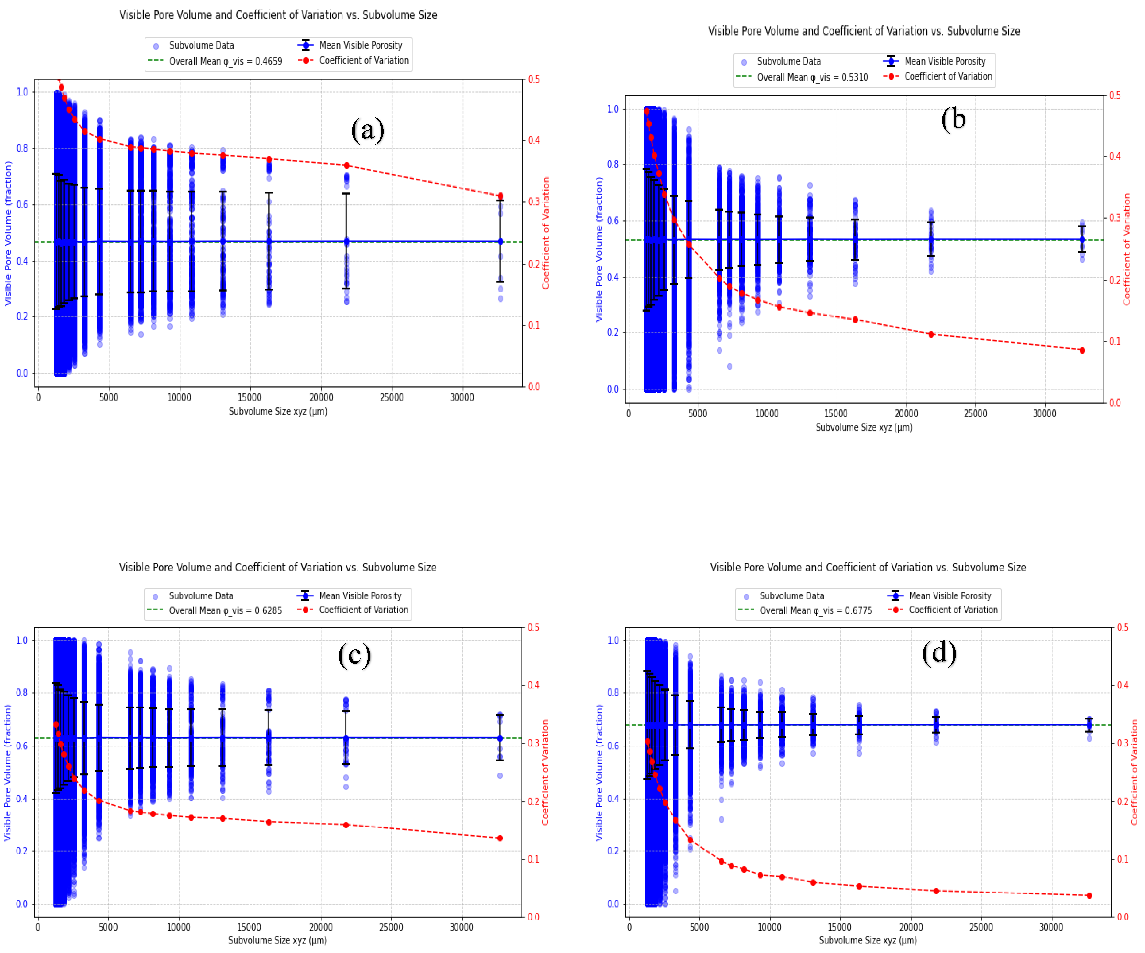
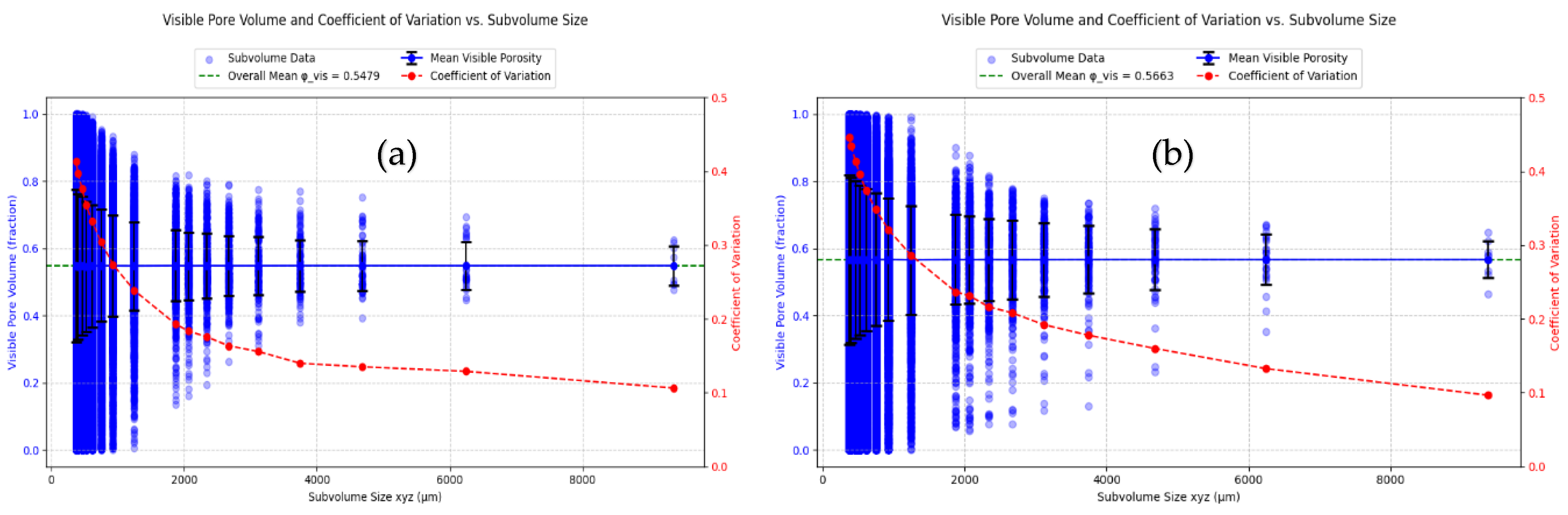
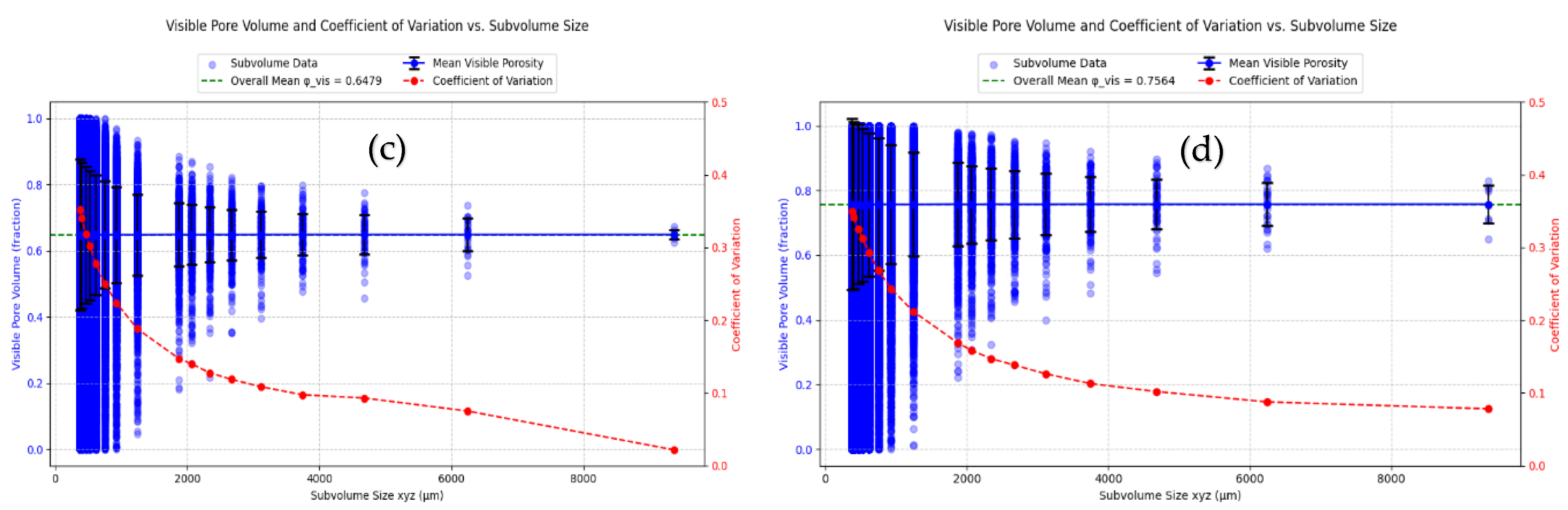
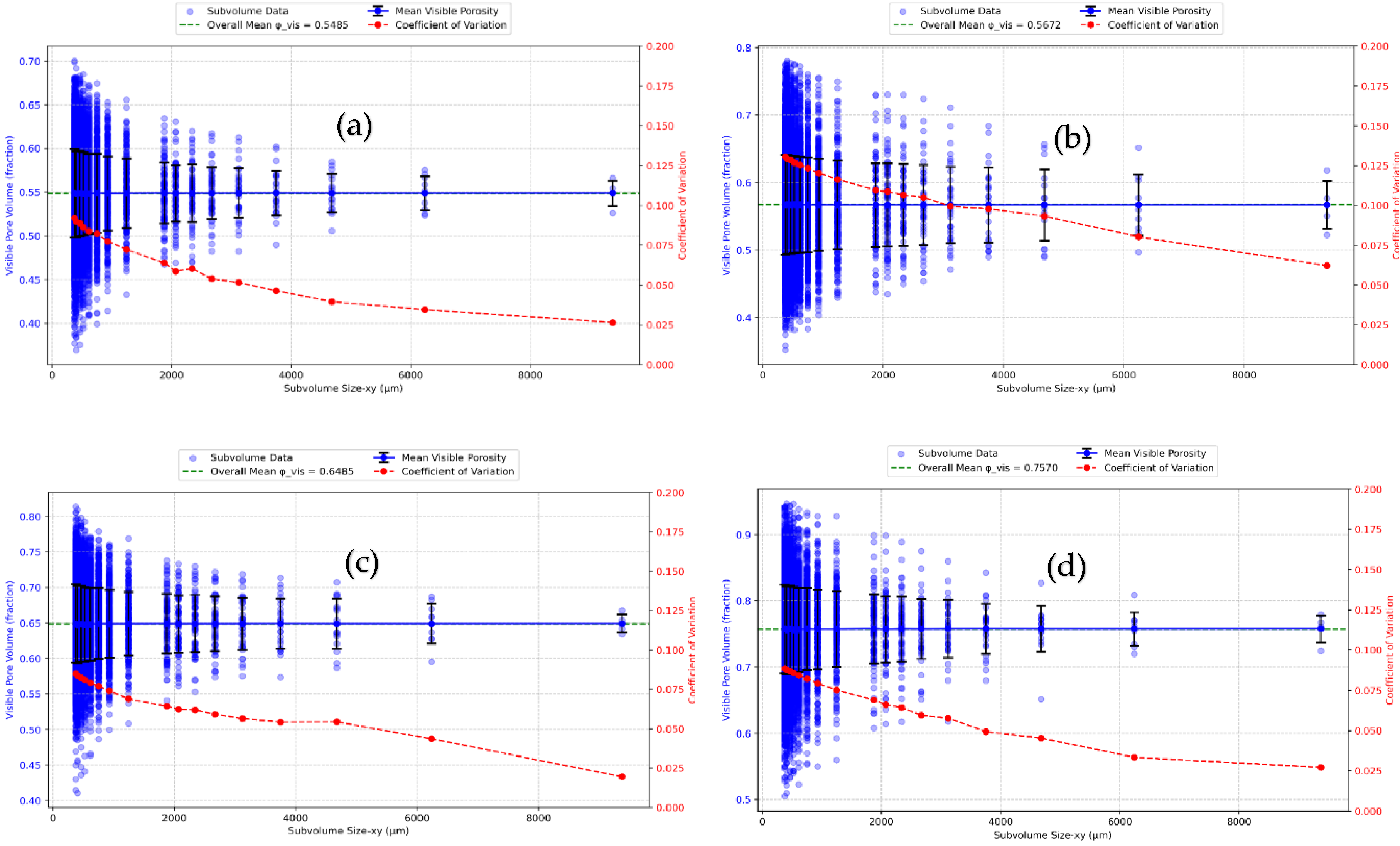
3.1. Analysis of REV

Figure 4a–d and Table 3 summarise the representative elementary volume analysis using two complementary criteria. The sREV is identified when the coefficient of variation stabilises below a fixed threshold as subvolume edge length increases, and the dREV is identified when at least three consecutive subvolumes show minimal change in visible porosity. In the 3D division of the large samples, all materials display pronounced variability at small edge lengths. Peat and RHP15 converge only slowly, WF4-50 shows comparable behaviour, and only WF4-100 satisfies both criteria. Because the dual criteria are not fulfilled consistently across materials in this configuration, we did not pursue three-dimensional division of the large samples further; detailed thresholds are reported in Table 3.
A slight vertical compaction gradient was unavoidable despite careful packing and handling, which increases visible porosity near the cylinder top and inflates variability when the depth is partitioned. To minimise this effect, we repeated the analysis with a two-dimensional division in which the full depth remains intact and tiling is performed only in the x and y directions. Under this configuration (Figure 5a–d), all four materials meet both criteria within the mesoscale range, and the variability of subvolume porosity is markedly reduced relative to the three-dimensional division. For subsequent analyses on large samples, we therefore adopt an edge length of 20000 µm.
For the small samples, the higher resolution and smaller physical extent shift the relevant scales downward. In the three-dimensional division (Figure 6a–d), residual heterogeneity still prevents a universal REV; only WF4-50 meets both criteria, whereas Peat, RHP15, and WF4-100 show non-overlapping ranges for the statistical and deterministic criteria. When the depth is kept intact and only the x and y directions are tiled (Figure 7a–d), all materials satisfy both criteria within a narrow lower-mesoscale band. We therefore use an edge length of 6000 µm for subsequent analyses on the small samples.
Taken together, these results show that keeping the full depth improves the robustness of REV detection in the presence of weak vertical gradients and yields material-consistent scales for downstream pore-structure metrics and hydraulic modelling. The adopted edge lengths of 20000 µm for large cylinders and 6000 µm for small cylinders ensure that all subsequent analyses are performed on statistically representative subvolumes. Exact thresholds per material and division mode are provided in Table 3.

3.2. Pore Structure Measures

Figure 8 shows the pore morphological properties, including pore volume, pore surface density, mean pore curvature density, the pore topological properties (Euler characteristic density and gamma indicator), and the average and critical pore diameter.
The laboratory-measured expected porosity consistently exceeded the image-based visible porosity across most samples (Figure 8a, large samples, and 8b, small samples), suggesting that µCT-derived estimates systematically understate expected porosity because most of the fine pores fall below the imaging resolution threshold (e.g., [72,73]). In the case of large images, samples RHP15 and WF4-50 exhibited minimal discrepancy between the two approaches, indicating good agreement for these relatively more homogeneous and coarse-textured media. In contrast, Peat and WF4-100 showed marked underestimation in image-based porosity, likely due to the exclusion of sub-voxel-scale pores during segmentation. Thresholding biases during image processing commonly documented as a source of visible porosity underestimation further exacerbate this effect, particularly in heterogeneous materials like peat (e.g., [74]). All small-image samples demonstrated lower image-based porosity compared to expected laboratory values, with the discrepancy more pronounced than in larger images. This pattern underscores the influence of the field of view and limited sampling of denser regions may bias image-derived porosity downward. The close match between image- and lab-based porosity for RHP15 and WF4-50 in large images suggested that a more uniform pore structure and fewer fine voids enhance µCT performance. Overall, these findings strongly affirmed that voxel resolution, segmentation threshold choice, and image volume critically affect the accuracy of µCT-based porosity estimation, particularly for fine-textured or highly heterogeneous growing media.
The comparison between large and small samples with the different resolutions (Figure 8c and 8d) revealed systematic differences in pore surface density and mean curvature density across all materials. Small samples consistently showed higher pore surface density than large samples, in some cases more than double. This is likely due to the higher resolution when imaging smaller volumes, which allows a more accurate capture of fine meso- and micro-pores [75,76]. In contrast, large samples tended to exhibit higher mean curvature densities than small samples, suggesting that larger volumes capture a more complete representation of complex three-dimensional pore–solid interfaces, including macro-pore features that may be underrepresented in small volumes [77]. Among the materials analysed, peat exhibited the highest mean curvature density in both large and small datasets. This reflects the inherently intricate and heterogeneous pore geometry of peat-dominant medium, often characterised by irregular voids and highly tortuous surfaces [78]. The consistently positive curvature values in all cases indicated predominantly convex interface shapes, which may correspond to bubble-like or spherical pores embedded in the matrix [79]. From a functional perspective, pore surface density and curvature are mechanistic controls rather than mere descriptors and higher surface density increases solid-liquid interfacial area, which can enhance capillarity and water retention in fine pores but also accelerate drying by enlarging the evaporative interface [80]. Curvature plays a key role in controlling capillary pressure, as described by the Young–Laplace equation: pores with high positive curvature (convex surfaces) tend to hold water at higher tensions, which influences the shape of water retention curves. The increased interfacial area associated with high surface density can promote greater solute adsorption and facilitate diffusive exchange between pore water and the solid phase [81,82]. However, highly tortuous, high-curvature surfaces may also create micro-domains of slow flow, leading to solute trapping and delayed breakthrough in leaching scenarios. Large, interconnected macro-pores typically have lower curvature values and dominate oxygen diffusion and CO₂ release in porous media [83]. Conversely, high-curvature small pores may remain water-filled under typical irrigation regimes, limiting gaseous exchange and potentially creating localised anaerobic conditions that impact root respiration and microbial activity. The observed differences highlight a fundamental trade-off in µCT-based pore characterisation as small samples enhance the detection of fine-scale surface features due to higher resolution, while larger volumes yield a more statistically representative measure of overall structural complexity. These findings reinforce the need for careful selection of sample size and voxel resolution in quantitative analysis of porous media, particularly when parameters such as surface density and curvature are used in hydraulic modelling, solute transport predictions, or assessments of aeration status in growing substrates.
The Euler characteristic density and probability of connectivity or gamma indicator (γ) revealed distinct differences in the pore network structure of the growing media (Figure 8e and 8f). The Euler characteristic density of the small samples is markedly more negative than that of the large samples, indicating a higher degree of pore connectivity [3,34]. Highly negative Euler values suggested fewer isolated pores and more continuous pathways, which is beneficial for fluid transport. The γ values for all samples, both large and small, are close to 1 (0.997–1.000), demonstrating that the pore networks are well connected. This high connectivity is crucial for maintaining efficient water flow, solute transport, and gas exchange in growing media [84,85]. In particular, high pore connectivity reduces the risk of waterlogging and improves oxygen diffusion to plant roots, while facilitating nutrient mobility. The combination of highly negative Euler values and γ ≈ 1 indicates that all media types have robust, percolating pore networks, although the small samples tend to show more interconnected pores at the microstructural level due to their higher resolution, potentially influencing hydraulic conductivity and aeration capacity.
The average pore diameter (mean pore size) was consistently largest in WF4-100 and smallest in Peat across both large and small image volumes (Figure 8g), indicating that wood fibre–rich media exhibit coarser pore structures compared to Peat. The critical pore diameter representing the largest pore necks and governing hydraulic continuity, was also greatest in WF4-100 and lowest in Peat (Figure 8h), with small-sample measurements generally yielding much smaller values than large-sample analyses. Functionally, larger pore diameters facilitate rapid drainage and low capillary retention, promoting hydraulic conductivity, but may reduce water storage capacity, aligning with the water retention curve (WRC) theory that links pore size to matric suction via the Young–Laplace equation [86]. The finer pores observed in peat likely enhance water retention and reduce hydraulic conductivity (see section (3.4)), whereas larger critical pore sizes in WF4-100 suggested improved aeration and lower risk of waterlogging, a key consideration for growing media design. The marked reductions in critical pore diameter for small-sample segments underscore the importance of imaging volume on hydraulic interpretation, underestimations could misrepresent gravity-driven flow pathways in µCT analyses. Overall, the pore diameter metrics reinforce the trade-offs between retention, drainage, and aeration in substrate selection, underscored by fundamental soil physics relationships.

3.3. Water Retention Curve

The water retention curves (WRCs) derived from the µCT image analysis for large and small samples were compared with the laboratory-measured WRC (both estimated continuous curves and discrete measurement points) for the four growing media (Figure 9). Across all materials, the laboratory-estimated WRCs showed the expected S-shaped retention behaviour, with high water contents at low matric potentials (low pF) and a progressive decline as pF increased. However, the image-derived WRCs deviated from laboratory measurements to varying extents, with discrepancies influenced by both material type and image volume.
For Peat and RHP15, the large-sample WRCs tended to slightly underestimate water content at intermediate suction ranges (pF ≈ 1–2), while overestimating water content near saturation compared to laboratory measurements. Small-sample WRCs, in contrast, often overestimated intermediate-range water contents but showed closer agreement near saturation. This divergence is likely due to differences in the ability of small and large sample volumes to capture the full range of macro- and mesopores. Larger sample volumes capture more structural heterogeneity and macro-pore pathways, which drain rapidly and thus lower the predicted water contents in the mid-suction range. Smaller sample volumes, particularly if dominated by finer pore regions, may overestimate water retention due to reduced representation of gravity-driven drainage pathways.
For WF4-50, both large- and small-sample WRCs aligned relatively well with the laboratory curve in the high water content range (pF < 1), but large-sample results showed underestimations at intermediate suctions. The small-sample WRC remained higher than the large-sample WRC at pF ≈ 1–2, again indicating the influence of sample size on capturing connected macro-pores. This behaviour supports earlier findings that insufficient sample volume in μCT analyses can misrepresent preferential drainage networks, particularly those associated with gravity-driven flow [75,87].
For WF4-100, differences between image-derived and laboratory WRCs were smaller, especially in the intermediate and high pF ranges. Both large and small sample WRCs followed similar trends, suggesting that pore size distribution in this material is more homogeneous, reducing the impact of scanning resolution. However, the large sample still predicted slightly lower water contents at intermediate suctions, reflecting a better representation of larger, well-connected pores.
Overall, the results confirm that image volume (with resolution value) significantly affects μCT-derived WRCs. Larger volumes are more likely to include representative distributions of macro-pores and associated gravity-driven flow pathways, which drain at low suctions and reduce water retention estimates. Smaller sample volumes may bias results towards higher retention if macro-pore representation is limited. These findings are consistent with previous studies showing that sample size and structural heterogeneity influence the accuracy of μCT-derived hydraulic parameters [88,89]. Therefore, while μCT-based WRC estimation is a powerful non-destructive tool with R2 higher than 0.9 across all the samples, care must be taken to select an image volume that adequately captures the pore network relevant to water retention, drainage, and associated gas exchange dynamics in growing media. The results indicate that the images with higher resolution can capture more pores, which in turn, they contribute to a more extended WRCs.

3.4. Estimation of Saturated Hydraulic Conductivity

The saturated hydraulic conductivity (Ksat) was estimated using a pore network model (PNM). The PNM simulations were conducted on subsections of a large sample (divided into upper, middle, and lower parts) and on separate small samples for each sample. The REV results suggested the edge length of 20000 µm for large samples with the total image depth and the edge length of 6000 µm for small samples with the total image depth. However, processing the images with total image depth is computationally expensive. Therefore, the large images were divided into three subsections, whereas the middle of the small sample was used for the Ksat estimation.
These estimates were compared to laboratory-measured Ksat values obtained through standard methods (constant head). The results are visualised in a bar chart (Figure 10).
For the Peat sample, PNM estimates from the large image subsections, each subsection with 20000 µm edge length, showed consistent values without statistical differences: 0.086 cm.s-1 (upper part), 0.109 cm.s-1 (middle part), and 0.079 cm.s-1 (lower part). The small sample yielded a lower Ksat of 0.051 cm.s-1, which differed from the laboratory measurement of 0.041 cm.s-1 by 25%, indicating a moderate overestimation. This suggests potential limitations in capturing fine porosity at the larger scale. In the RHP15 sample, the large sample parts exhibited Ksat values of 0.0841 cm.s-1 (upper), 0.140 cm.s-1 (middle), and 0.132 cm.s-1 (lower), with minimal variation among them. The small sample estimate was 0.121 cm.s-1 , differing from the lab-measured 0.044 cm.s-1 by 172%, pointing to a significant overestimation.
For WF4-50, the large sample estimates were 0.112 cm.s-1 (upper), 0.143 cm.s-1 (middle), and 0.166 cm.s-1 (lower), showing a slight increasing trend from upper to lower, possibly due to subtle structural gradients. The small sample provided 0.141 cm.s-1, which differed from the lab value of 0.228 cm.s-1 by -38%, indicating an underestimation. This suggested variable performance across material types. Finally, for WF4-100, the large sample subsections yielded low values: 0.061 cm.s-1 (upper), 0.097 cm.s-1 (middle), and 0.112 cm.s-1 (lower). The small sample estimate was 0.682 cm.s-1, differing from the lab measurement of 0.562 cm.s-1 by 21%, reflecting the method's efficacy for coarser materials.
The consistency among the upper, middle, and lower parts of the large samples within each sample indicates homogeneity in the modelled pore networks at that scale. This could be attributed to the applied pressure gradient in PNM simulations dominating over minor porosity variations. However, the overestimation observed in large sample subsections for lower-Ksat materials like Peat and RHP15 highlights potential issues, such as insufficient resolution to resolve fine pores or artefacts from image segmentation, leading to artificially enhanced connectivity. In contrast, small samples, likely acquired at higher magnification, yielded Ksat values in better agreement with laboratory measurements, with relative discrepancies ranging from 21% to 172% across samples (with underestimation of 38% in WF4-50), likely due to enhanced detail in capturing microporosity critical for organic-rich media. This aligns with findings that higher-resolution imaging reduces errors in PNM for estimating saturated conductivity [90].
The PNM approach offers a non-invasive, image-based method to estimate Ksat by simulating fluid flow through extracted pore networks, capturing microstructural details like pore size distribution and throat connectivity [91]. The tendency to improved fidelity of small sample estimates suggested that higher-resolution imaging better resolves key flow paths, particularly for lower-permeability media. For higher-conductivity samples (e.g., WF4-100), the PNM estimates from small samples deviated only slightly from lab values, underscoring the method's reliability for materials with coarser pore structures. Compared to other models [90], intercomparisons showed PNM provides statistically equivalent Ksat to more computationally intensive Navier-Stokes approaches, with no significant discrepancies, while empirical equations like Kozeny-Carman may vary in accuracy due to unaccounted factors.
Comparisons in other studies revealed that PNM tends to overestimate Ksat in low-permeability media relative to lab values, possibly due to assumptions like Poiseuille flow in throats or neglecting surface roughness, which may not fully replicate real-world conditions; simplified geometries in PNM can introduce minor biases, though overall credibility depends on accurate pore space representation from experimental data [91]. Future refinements could involve multi-scale imaging to bridge large and small sample discrepancies, or integrating machine learning for better segmentation and direct Ksat prediction using techniques like neural networks or random forests, which have shown efficacy in modelling hydraulic properties from porous media data [92]. Overall, PNM provides valuable insights into microstructural controls on hydraulic properties, with small-scale imaging enhancing its predictive accuracy for diverse growing media. This has implications for optimising substrates in horticulture and hydrology, where rapid, non-destructive assessments are advantageous.

4. Conclusions

This study has successfully elucidated the representative elementary volume (REV) for visible porosity in various horticultural growing media namely Peat, RHP15, WF4-50, and WF4-100 using µCT imaging at different scales and division methods, while also evaluating pore morphological and topological properties, water retention curves (WRCs), and saturated hydraulic conductivity (Ksat) through pore network modelling (PNM). The main findings revealed that REV determination is highly dependent on the image division approach and sample size. For 3D division of the large images, REV was achieved only for WF4-100 based on dual criteria (deterministic REV [dREV] and statistical REV [sREV]), with subvolume sizes ranging from 8000 to 10000 µm, highlighting the intrinsic heterogeneity of other media like Peat, RHP15, and WF4-50, where criteria were not simultaneously met due to pronounced porosity fluctuations at microscales (<5000 µm). In contrast, 2D division of large images yielded REV for all media within 13000 to 21000 µm, exhibiting reduced variability and better stability, attributed to the inclusion of full image depth. For small images, 3D division met dual criteria only for WF4-50 (REV 3000–6000 µm), while 2D division succeeded for all materials, underscoring the superiority of 2D approaches in capturing mesoscale homogeneity. Pore analyses further demonstrated that laboratory-measured porosity consistently exceeded µCT-derived visual porosity values, with discrepancies minimised in homogeneous media (e.g., RHP15, WF4-50), due to resolution limitations excluding sub-voxel pores. Small images showed higher pore surface density but lower mean curvature density than large images, reflecting enhanced fine-pore detection at higher resolutions, with peat exhibiting the most complex structures. Topological metrics indicated highly connected networks (γ ≈ 1, negative Euler densities), particularly in small samples, promoting efficient transport. Pore sizes were largest in WF4-100 and smallest in Peat, influencing drainage and retention. Image-derived WRCs aligned well with laboratory data (R² > 0.9), though small images overestimated retention at intermediate suctions (pF 1–2) due to limited macro-pore representation, while large images better captured drainage pathways. PNM-estimated Ksat from small images showed closer agreement with lab values (discrepancies 21–172%), outperforming large-image subsections, which overestimated in low-permeability media like Peat and RHP15, likely from image resolutions.
These findings directly align with the study's objectives to determine REV for porosity in growing media via µCT, compare image- and lab-based hydrophysical properties, and assess PNM for Ksat prediction. By establishing REV scales, the research provides a framework for selecting representative sample volumes that minimise variability in porosity measurements, ensuring reliable characterisation of pore networks critical for hydraulic behaviour. The observed trade-offs—e.g., higher porosity and connectivity in wood fibre-rich media (WF4-100) versus finer, retentive structures in peat inform substrate optimisation for water management, aeration, and nutrient transport in horticulture, supporting sustainable alternatives to peat-based media. Moreover, the validation of µCT and PNM as non-destructive tools advances multiscale imaging for predicting functional properties, bridging microstructural details to macroscopic performance as per Young–Laplace and Darcy's principles.
Despite these contributions, the study is limited by determining REV solely based on visible porosity, potentially overlooking other parameters that could yield different REV scales. Future work should extend REV assessments to permeability or tortuosity, which may better capture flow dynamics in heterogeneous media. Additionally, while PNM demonstrated utility for Ksat estimation, comparative evaluations with advanced models such as Lattice Boltzmann Method (LBM) [93,94] or numerical finite element approaches [95] could reveal discrepancies in handling complex geometries and multiphase flows, enhancing model selection for hydraulic simulations. Finally, testing varied sample scales and image resolutions would address resolution-induced biases in pore detection, enabling more robust multiscale analyses and improved accuracy in hydrophysical predictions for diverse growing substrates.
Compared to standard laboratory methods, this study shows what µCT may uniquely add for growing media research: an image-based REV, quantitative interfacial geometry, explicit connectivity, and percolating throat sizes that link structure to function. These descriptors enable mechanism-based interpretation of WRCs and image driven Ksat estimates, and they reveal depth dependent compaction that remains hidden to standard methods.

Author Contributions

Conceptualization, H.H.M.; methodology, H.H.M. and R.A.; validation, K.K., M.S.R. and R.A.; formal analysis, H.H.M.; investigation, R.A.; writing—original draft preparation, H.H.M.; writing—review and editing, H.H.M., R.A., K.K., and M.S.R.; visualization, R.A.; supervision, R.A.; project administration, D.D.; funding acquisition, D.D. All authors have read and agreed to the published version of the manuscript

Funding

The study was partly financed by the German Federal Ministry of Food and Agriculture (BMEL), Project promotor FNR, Project NaKuHo, FKZ 2220MT001A.

Institutional Review Board Statement

Not applicable

Informed Consent Statement

Not applicable

Data Availability Statement

Data supporting this work will be made available upon request.

Conflicts of Interest

The authors declare that they have no known competing financial interests or personal relationships that could have appeared to influence the work reported in this paper.

References

  1. Helliwell, J.R.; Sturrock, C.J.; Grayling, K.M.; Tracy, S.R.; Flavel, R.J.; Young, I.M.; Whalley, W.R.; Mooney, S.J. Applications of X -ray computed tomography for examining biophysical interactions and structural development in soil systems: a review. European J Soil Science 2013, 64, 279–297. [Google Scholar] [CrossRef]
  2. Zong, Y.; Yu, X.; Zhu, M.; Lu, S. Characterizing soil pore structure using nitrogen adsorption, mercury intrusion porosimetry, and synchrotron-radiation-based X-ray computed microtomography techniques. J Soils Sediments 2015, 15, 302–312. [Google Scholar] [CrossRef]
  3. Vogel, H.-J.; Weller, U.; Schlüter, S. Quantification of soil structure based on Minkowski functions. Computers & Geosciences 2010, 36, 1236–1245. [Google Scholar] [CrossRef]
  4. Soracco, C.G.; Villarreal, R.; Melani, E.M.; Oderiz, J.A.; Salazar, M.P.; Otero, M.F.; Irizar, A.B.; Lozano, L.A. Hydraulic conductivity and pore connectivity. Effects of conventional and no-till systems determined using a simple laboratory device. Geoderma 2019, 337, 1236–1244. [Google Scholar] [CrossRef]
  5. Chamindu Deepagoda, T.; Chen Lopez, J.C.; Møldrup, P.; Jonge, L.W. de; Tuller, M. Integral parameters for characterizing water, energy, and aeration properties of soilless plant growth media. Journal of Hydrology 2013, 502, 120–127. [Google Scholar] [CrossRef]
  6. Müller, K.; Katuwal, S.; Young, I.; McLeod, M.; Moldrup, P.; Jonge, L.W. de; Clothier, B. Characterising and linking X-ray CT derived macroporosity parameters to infiltration in soils with contrasting structures. Geoderma 2018, 313, 82–91. [Google Scholar] [CrossRef]
  7. Gong, L.; Nie, L.; Xu, Y.; Ji, X.; Liu, B. Characterization of Micro-Scale Pore Structure and Permeability Simulation of Peat Soil Based on 2D/3D X-ray Computed Tomography Images. Eurasian Soil Sc. 2022, 55, 790–801. [Google Scholar] [CrossRef]
  8. DIN 19683. Methods of Soil Investigations for agricultural engineering – Physical laboratory tests- part9 : Determination of the saturated hydraulic water conductivity in the cylindrical core-cutter; 1998.
  9. DIN EN 13041. Soil Improvers and Growing Media-Determination of Physical Properties-Dry Bulk Density, Air Volume, Water Volume, Shrinkage Value and Total Pore Space; 2011.
  10. DIN EN ISO 11274. Soil quality – Determination of the water-retention characteristic – Laboratory methods. 1127.
  11. Muhammed, H.H.; Schumm, L.; Anlauf, R.; Reineke, T.; Daum, D. Validity of a Centrifuge-Based Method for Determining the Water Retention Curve of Growing Media. Horticulturae 2024, 10, 1255. [Google Scholar] [CrossRef]
  12. Fields, J.S.; Owen, J.S.; Stewart, R.D.; Heitman, J.L.; Caron, J. Modeling water fluxes through containerized soilless substrates using HYDRUS. Vadose Zone Journal 2020, 19. [Google Scholar] [CrossRef]
  13. Anlauf, R.; Rehrmann, P.; Schacht, H. Simulation of water uptake and redistribution in growing media during ebb-and-flow irrigation. Journal of Horticulture and Forestry 2012, 4, 8–21. [Google Scholar] [CrossRef]
  14. Anlauf, R.; Muhammed, H.H.; Reineke, T.; Daum, D. Water retention properties of wood fiber based growing media and their impact on irrigation strategy. 2023. [CrossRef]
  15. Muhammed, H.H.; Anlauf, R.; Daum, D. Estimation of Hydraulic Properties of Growing Media from Numerical Inversion of Mini Disk Infiltrometer Data. Hydrology 2025, 12, 100. [Google Scholar] [CrossRef]
  16. Kuka, K.; Illerhaus, B.; Fox, C.A.; Joschko, M. X-ray computed microtomography for the study of the soil–root relationship in grassland soils. Vadose Zone Journal 2013, 12, vzj2013–01.0014. [Google Scholar] [CrossRef]
  17. Kuka, K.; Joschko, M. Grassland management intensity determines root development, soil structure, and their interrelationship: Results of a regional study of Leptosols in the Swabian Alps. Grassland Research 2024, 3, 171–186. [Google Scholar] [CrossRef]
  18. Fomin, D.S.; Yudina, A.V.; Romanenko, K.A.; Abrosimov, K.N.; Karsanina, M.V.; Gerke, K.M. Soil pore structure dynamics under steady-state wetting-drying cycle. Geoderma 2023, 432, 116401. [Google Scholar] [CrossRef]
  19. Houston, A.N.; Otten, W.; Falconer, R.; Monga, O.; Baveye, P.C.; Hapca, S.M. Quantification of the pore size distribution of soils: Assessment of existing software using tomographic and synthetic 3D images. Geoderma 2017, 299, 73–82. [Google Scholar] [CrossRef]
  20. Peters, A.; Hohenbrink, T.L.; Iden, S.C.; Durner, W. A simple model to predict hydraulic conductivity in medium to dry soil from the water retention curve. Water Resources Research 2021, 57, e2020WR029211. [Google Scholar] [CrossRef]
  21. Pires, L.F.; Auler, A.C.; Roque, W.L.; Mooney, S.J. X-ray microtomography analysis of soil pore structure dynamics under wetting and drying cycles. Geoderma 2020, 362, 114103. [Google Scholar] [CrossRef]
  22. Rijfkogel, L.S.; Ghanbarian, B.; Hu, Q.; Liu, H.-H. Clarifying pore diameter, pore width, and their relationship through pressure measurements: A critical study. Marine and Petroleum Geology 2019, 107, 142–148. [Google Scholar] [CrossRef]
  23. Zhang, Y.; Yang, Z.; Wang, F.; Zhang, X. Comparison of soil tortuosity calculated by different methods. Geoderma 2021, 402, 115358. [Google Scholar] [CrossRef]
  24. Munkholm, L.J.; Heck, R.J.; Deen, B. Soil pore characteristics assessed from X-ray micro-CT derived images and correlations to soil friability. Geoderma 2012, 181-182, 22–29. [Google Scholar] [CrossRef]
  25. Ju, X.; Jia, Y.; Li, T.; Gao, L.; Gan, M. Morphology and multifractal characteristics of soil pores and their functional implication. CATENA 2021, 196, 104822. [Google Scholar] [CrossRef]
  26. Torre, I.G.; Losada, J.C.; Heck, R.J.; Tarquis, A.M. Multifractal analysis of 3D images of tillage soil. Geoderma 2018, 311, 167–174. [Google Scholar] [CrossRef]
  27. Sun, X.; She, D.; Sanz, E.; Martín-Sotoca, J.J.; Tarquis, A.M.; Gao, L. Multifractal analysis on CT soil images: Fluctuation analysis versus mass distribution. Chaos, Solitons & Fractals 2023, 176, 114080. [Google Scholar] [CrossRef]
  28. Mady, A.Y.; Shein, E.V.; Abrosimov, K.N.; Skvortsova, E. X-ray computed tomography: Validation of the effect of pore size and its connectivity on saturated hydraulic conductivity. Soil & Environment 2021, 40. [Google Scholar] [CrossRef]
  29. Wildenschild, D.; Sheppard, A.P. X-ray imaging and analysis techniques for quantifying pore-scale structure and processes in subsurface porous medium systems. Advances in Water Resources 2013, 51, 217–246. [Google Scholar] [CrossRef]
  30. Weller, U.; Albrecht, L.; Schlüter, S.; Vogel, H.-J. An open Soil Structure Library based on X-ray CT data. Soil 2022, 8, 507–515. [Google Scholar] [CrossRef]
  31. Kalnin, T.G.; Ivonin, D.A.; Abrosimov, K.N.; Grachev, E.A.; Sorokina, N.V. Analysis of Tomographic Images of the Soil Pore Space Structure by Integral Geometry Methods. Eurasian Soil Sc. 2021, 54, 1400–1409. [Google Scholar] [CrossRef]
  32. Köhne, J.M.; Schlüter, S.; Vogel, H.-J. Predicting Solute Transport in Structured Soil Using Pore Network Models. Vadose Zone Journal 2011, 10, 1082–1096. [Google Scholar] [CrossRef]
  33. Tracy, S.R.; Daly, K.R.; Sturrock, C.J.; Crout, N.M.J.; Mooney, S.J.; Roose, T. Three-dimensional quantification of soil hydraulic properties using X-ray Computed Tomography and image-based modeling. Water Resources Research 2015, 51, 1006–1022. [Google Scholar] [CrossRef]
  34. Armstrong, R.T.; McClure, J.E.; Robins, V.; Liu, Z.; Arns, C.H.; Schlüter, S.; Berg, S. Porous media characterization using Minkowski functionals: Theories, applications and future directions. Transport in Porous Media 2019, 130, 305–335. [Google Scholar] [CrossRef]
  35. Koestel, J.; Larsbo, M.; Jarvis, N. Scale and REV analyses for porosity and pore connectivity measures in undisturbed soil. Geoderma 2020, 366, 114206. [Google Scholar] [CrossRef]
  36. Borges, J.A.R.; Pires, L.F.; Cássaro, F. am; Roque, W.L.; Heck, R.J.; Rosa, J.A.; Wolf, F.G. X-ray microtomography analysis of representative elementary volume (REV) of soil morphological and geometrical properties. Soil and Tillage Research 2018, 182, 112–122. [Google Scholar] [CrossRef]
  37. Gaspareto, J.V.; Oliveira, J.A.T. de; Andrade, E.; Pires, L.F. Representative Elementary Volume as a Function of Land Uses and Soil Processes Based on 3D Pore System Analysis. Agriculture 2023, 13, 736. [Google Scholar] [CrossRef]
  38. Koestel, J.; Larsbo, M.; Jarvis, N. Scale and REV analyses for porosity and pore connectivity measures in undisturbed soil. Geoderma 2020, 366, 114206. [Google Scholar] [CrossRef]
  39. Turunen, M.; Hyväluoma, J.; Heikkinen, J.; Keskinen, R.; Kaseva, J.; Koestel, J.; Rasa, K. Quantifying Physical Properties of Three Sphagnum -Based Growing Media as Affected by Drying–Wetting Cycles. Vadose Zone Journal 2019, 18. [Google Scholar] [CrossRef]
  40. Quinton, W.L.; Elliot, T.; Price, J.S.; Rezanezhad, F.; Heck, R. Measuring physical and hydraulic properties of peat from X-ray tomography. Geoderma 2009, 153, 269–277. [Google Scholar] [CrossRef]
  41. VDLUFA, 1991. VDLUFA (Association of German Agricultural Analytic and Research Institutes) (1991) Methods Book I "Soil Analysis" (1st-6th supplement delivery), 4th edn. VDLUFA-Verlag, Darmstadt.
  42. DIN EN 13039. Soil Improvers and growing media – Determination of organic content and ash. German Version.; 2009.
  43. Kemper, W.D.; Rosenau, R.C. Aggregate stability and size distribution. Methods of soil analysis: Part 1 Physical and mineralogical methods 1986, 5, 425–442. [Google Scholar] [CrossRef]
  44. van Genuchten, M.T. A closed-form equation for predicting the hydraulic conductivity of unsaturated soils. Soil Science Society of America Journal 1980, 44, 892–898. [Google Scholar] [CrossRef]
  45. Borges, J.A.R.; Pires, L.F.; Cássaro, F. am; Roque, W.L.; Heck, R.J.; Rosa, J.A.; Wolf, F.G. X-ray microtomography analysis of representative elementary volume (REV) of soil morphological and geometrical properties. Soil and Tillage Research 2018, 182, 112–122. [Google Scholar] [CrossRef]
  46. Gaspareto, J.V.; Oliveira, J.A.T. de; Andrade, E.; Pires, L.F. Representative Elementary Volume as a Function of Land Uses and Soil Processes Based on 3D Pore System Analysis. Agriculture 2023, 13, 736. [Google Scholar] [CrossRef]
  47. Kettridge, N.; Binley, A. Characterization of peat structure using X-ray computed tomography and its control on the ebullition of biogenic gas bubbles. Journal of Geophysical Research: Biogeosciences 2011, 116. [Google Scholar] [CrossRef]
  48. San José Martínez, F.; Martín, L.; García-Gutiérrez, C. Minkowski functionals of connected soil porosity as indicators of soil tillage and depth. Frontiers in Environmental Science 2018, 6, 55. [Google Scholar] [CrossRef]
  49. Harris, C.R.; Millman, K.J.; van der Walt, S.J.; Gommers, R.; Virtanen, P.; Cournapeau, D.; Wieser, E.; Taylor, J.; Berg, S.; Smith, N.J.; et al. Array programming with NumPy. Nature 2020, 585, 357–362. [Google Scholar] [CrossRef]
  50. Hunter, J.D. Matplotlib: A 2D graphics environment. Computing in science & engineering 2007, 9, 90–95. [Google Scholar] [CrossRef]
  51. van der Walt, S.; Schönberger, J.L.; Nunez-Iglesias, J.; Boulogne, F.; Warner, J.D.; Yager, N.; Gouillart, E.; Yu, T. scikit-image: image processing in Python. PeerJ 2014, 2, e453. [Google Scholar] [CrossRef]
  52. Virtanen, P.; Gommers, R.; Oliphant, T.E.; Haberland, M.; Reddy, T.; Cournapeau, D.; Burovski, E.; Peterson, P.; Weckesser, W.; Bright, J.; et al. SciPy 1.0: fundamental algorithms for scientific computing in Python. Nature Methods 2020, 17, 261–272. [Google Scholar] [CrossRef]
  53. Christoph Gohlke. cgohlke/tifffile: v2025.6.11; 2025.
  54. Mafi, M.; Martin, H.; Cabrerizo, M.; Andrian, J.; Barreto, A.; Adjouadi, M. A comprehensive survey on impulse and Gaussian denoising filters for digital images. Signal Processing 2019, 157, 236–260. [Google Scholar] [CrossRef]
  55. Costanza-Robinson, M.S.; Estabrook, B.D.; Fouhey, D.F. Representative elementary volume estimation for porosity, moisture saturation, and air-water interfacial areas in unsaturated porous media: Data quality implications. Water Resources Research 2011, 47. [Google Scholar] [CrossRef]
  56. Nordahl, K.; Ringrose, P.S. Identifying the representative elementary volume for permeability in heterolithic deposits using numerical rock models. Mathematical geosciences 2008, 40, 753–771. [Google Scholar] [CrossRef]
  57. Wu, M.; Wu, J.; Wu, J.; Hu, B.X. A new criterion for determining the representative elementary volume of translucent porous media and inner contaminant. Hydrology and Earth System Sciences Discussions 2020, 2020, 1–41. [Google Scholar] [CrossRef]
  58. Borges, J.A.R.; Pires, L.F.; Belmont Pereira, A. Computed tomography to estimate the representative elementary area for soil porosity measurements. The Scientific World Journal 2012, 2012, 526380. [Google Scholar] [CrossRef]
  59. Zhang, D.; Zhang, R.; Chen, S.; Soll, W.E. Pore scale study of flow in porous media: Scale dependency, REV, and statistical REV. Geophysical Research Letters 2000, 27, 1195–1198. [Google Scholar] [CrossRef]
  60. Osher, S.; Sethian, J.A. Fronts propagating with curvature-dependent speed: Algorithms based on Hamilton-Jacobi formulations. Journal of computational physics 1988, 79, 12–49. [Google Scholar] [CrossRef]
  61. Sethian, J.A. Level set methods and fast marching methods; Cambridge Cambridge UP, 1999.
  62. Pabst, W.; Gregorová, E. Characterization of particles and particle systems. Available online: https://old.vscht.cz/sil/keramika/Characterization_of_particles/CPPS%20_English%20version_.pdf (accessed on 13 August 2025).
  63. Renard, P.; Allard, D. Connectivity metrics for subsurface flow and transport. Advances in Water Resources 2013, 51, 168–196. [Google Scholar] [CrossRef]
  64. Koestel, J.; Schlueter, S. Quantification of the structure evolution in a garden soil over the course of two years. Geoderma 2019, 338, 597–609. [Google Scholar] [CrossRef]
  65. Nishiyama, N.; Yokoyama, T. Permeability of porous media: Role of the critical pore size. Journal of Geophysical Research: Solid Earth 2017, 122, 6955–6971. [Google Scholar] [CrossRef]
  66. Hillel, D. Introduction to Environmental Soil Physics. Elsevier Academic Press, Amsterdam, 2004., 2005, 56 (5). 56.
  67. Gostick, J.T.; Khan, Z.A.; Tranter, T.G.; Kok, M.; Agnaou, M.; Sadeghi, M.; Jervis, R. PoreSpy: A python toolkit for quantitative analysis of porous media images. Journal of Open Source Software 2019, 4, 1296. [Google Scholar] [CrossRef]
  68. Bouix, S. , Siddiqi, K. Divergence-based medial surfaces 2000. [CrossRef]
  69. Gostick, J.; Aghighi, M.; Hinebaugh, J.; Tranter, T.; Hoeh, M.A.; Day, H.; Spellacy, B.; Sharqawy, M.H.; Bazylak, A.; Burns, A. OpenPNM: a pore network modeling package. Computing in science & engineering 2016, 18, 60–74. [Google Scholar] [CrossRef]
  70. Patzek, T.W.; Silin, D.B. Shape factor and hydraulic conductance in noncircular capillaries: I. One-phase creeping flow. Journal of colloid and interface science 2001, 236, 295–304. [Google Scholar] [CrossRef] [PubMed]
  71. Valvatne, P.H.; Blunt, M.J. Predictive pore-scale modeling of two-phase flow in mixed wet media. Water Resources Research 2004, 40. [Google Scholar] [CrossRef]
  72. Meira Cassaro, F.A.; Posadas Durand, A.N.; Gimenez, D.; Pedro Vaz, C.M. Pore-Size Distributions of Soils Derived using a Geometrical Approach and Multiple Resolution MicroCT Images. Soil Science Soc of Amer J 2017, 81, 468–476. [Google Scholar] [CrossRef]
  73. Beckers, E.; Plougonven, E.; Gigot, N.; Léonard, A.; Roisin, C.; Brostaux, Y.; Degré, A. Coupling X-ray microtomography and macroscopic soil measurements: a method to enhance near-saturation functions? Hydrology and Earth System Sciences 2014, 18, 1805–1817. [Google Scholar] [CrossRef]
  74. Ojeda-Magaña, B.; Quintanilla-Domínguez, J.; Ruelas, R.; am Tarquis; Gómez-Barba, L. ; Andina, D. Identification of pore spaces in 3D CT soil images using PFCM partitional clustering. Geoderma 2014, 217, 90–101. [Google Scholar] [CrossRef]
  75. Wildenschild, D.; Sheppard, A.P. X-ray imaging and analysis techniques for quantifying pore-scale structure and processes in subsurface porous medium systems. Advances in Water Resources 2013, 51, 217–246. [Google Scholar] [CrossRef]
  76. Houston, A.N.; Schmidt, S.; am Tarquis; Otten, W. ; Baveye, P.C.; Hapca, S.M. Effect of scanning and image reconstruction settings in X-ray computed microtomography on quality and segmentation of 3D soil images. Geoderma 2013, 207, 154–165. [Google Scholar] [CrossRef]
  77. Smet, S.; Plougonven, E.; Leonard, A.; Degré, A.; Beckers, E. X-ray µCT: how soil pore space description can be altered by image processing. Vadose Zone Journal 2018, 17. [Google Scholar] [CrossRef]
  78. Rezanezhad, F.; Price, J.S.; Craig, J.R. The effects of dual porosity on transport and retardation in peat: A laboratory experiment. Canadian Journal of Soil Science 2012, 92, 723–732. [Google Scholar] [CrossRef]
  79. Prodanović, M.; Lindquist, W.B.; Seright, R.S. 3D image-based characterization of fluid displacement in a Berea core. Advances in Water Resources 2007, 30, 214–226. [Google Scholar] [CrossRef]
  80. Or, D.; Smets, B.F.; Wraith, J.M.; Dechesne, A.; Friedman, S.P. Physical constraints affecting bacterial habitats and activity in unsaturated porous media–a review. Advances in Water Resources 2007, 30, 1505–1527. [Google Scholar] [CrossRef]
  81. Menon, M.; Jia, X.; Lair, G.J.; Faraj, P.H.; Blaud, A. Analysing the impact of compaction of soil aggregates using X-ray microtomography and water flow simulations. Soil and Tillage Research 2015, 150, 147–157. [Google Scholar] [CrossRef]
  82. Fukumasu, J.; Jarvis, N.; Koestel, J.; Larsbo, M. Links between soil pore structure, water flow and solute transport in the topsoil of an arable field: Does soil organic carbon matter? Geoderma 2024, 449, 117001. [Google Scholar] [CrossRef]
  83. Du, Y.; Guo, S.; Wang, R.; Song, X.; Ju, X. Soil pore structure mediates the effects of soil oxygen on the dynamics of greenhouse gases during wetting–drying phases. Science of The Total Environment 2023, 895, 165192. [Google Scholar] [CrossRef]
  84. Arthur, E.; Moldrup, P.; Schjønning, P.; Jonge, L.W. de. Water retention, gas transport, and pore network complexity during short-term regeneration of soil structure. Soil Science Soc of Amer J 2013, 77, 1965–1976. [Google Scholar] [CrossRef]
  85. Peth, S.; Horn, R.; Beckmann, F.; Donath, T.; Fischer, J.; Smucker, A.J. Three-dimensional quantification of intra-aggregate pore-space features using synchrotron-radiation-based microtomography. Soil Science Soc of Amer J 2008, 72, 897–907. [Google Scholar] [CrossRef]
  86. Hou, X.; Qi, S.; Liu, F. Soil water retention and pore characteristics of intact loess buried at different depths. Sustainability 2023, 15, 14890. [Google Scholar] [CrossRef]
  87. Blunt, M.J.; Bijeljic, B.; Dong, H.; Gharbi, O.; Iglauer, S.; Mostaghimi, P.; Paluszny, A.; Pentland, C. Pore-scale imaging and modelling. Advances in Water Resources 2013, 51, 197–216. [Google Scholar] [CrossRef]
  88. Baveye, P.C.; Laba, M.; Otten, W.; Bouckaert, L.; Sterpaio, P.D.; Goswami, R.R.; Grinev, D.; Houston, A.; Hu, Y.; Liu, J. Observer-dependent variability of the thresholding step in the quantitative analysis of soil images and X-ray microtomography data. Geoderma 2010, 157, 51–63. [Google Scholar] [CrossRef]
  89. Houston, A.N.; Otten, W.; Falconer, R.; Monga, O.; Baveye, P.C.; Hapca, S.M. Quantification of the pore size distribution of soils: Assessment of existing software using tomographic and synthetic 3D images. Geoderma 2017, 299, 73–82. [Google Scholar] [CrossRef]
  90. Gackiewicz, B.; Lamorski, K.; Sławiński, C.; Hsu, S.-Y.; Chang, L.-C. An intercomparison of the pore network to the Navier–Stokes modeling approach applied for saturated conductivity estimation from X-ray CT images. Sci. Rep. 2021, 11, 5859. [Google Scholar] [CrossRef]
  91. Xiong, Q.; Baychev, T.G.; Jivkov, A.P. Review of pore network modelling of porous media: Experimental characterisations, network constructions and applications to reactive transport. Journal of contaminant hydrology 2016, 192, 101–117. [Google Scholar] [CrossRef]
  92. Devi, A.; Chandel, A.; Shankar, V. Modelling hydraulic conductivity of porous media using machine learning techniques. Journal of Hydroinformatics 2025, 27, 381–405. [Google Scholar] [CrossRef]
  93. Foroughi, S.; Shojaei, M.J.; Lane, N.; Rashid, B.; Lakshtanov, D.; Ning, Y.; Zapata, Y.; Bijeljic, B.; Blunt, M.J. A framework for multiphase pore-scale modeling based on micro-CT imaging. Transport in Porous Media 2025, 152, 18. [Google Scholar] [CrossRef]
  94. Song, R.; Wang, Y.; Liu, J.; Cui, M.; Lei, Y. Comparative analysis on pore-scale permeability prediction on micro-CT images of rock using numerical and empirical approaches. Energy Science & Engineering 2019, 7, 2842–2854. [Google Scholar] [CrossRef]
  95. Callow, B.; Falcon-Suarez, I.; Marin-Moreno, H.; Bull, J.M.; Ahmed, S. Optimal X-ray micro-CT image based methods for porosity and permeability quantification in heterogeneous sandstones. Geophysical Journal International 2020, 223, 1210–1229. [Google Scholar] [CrossRef]
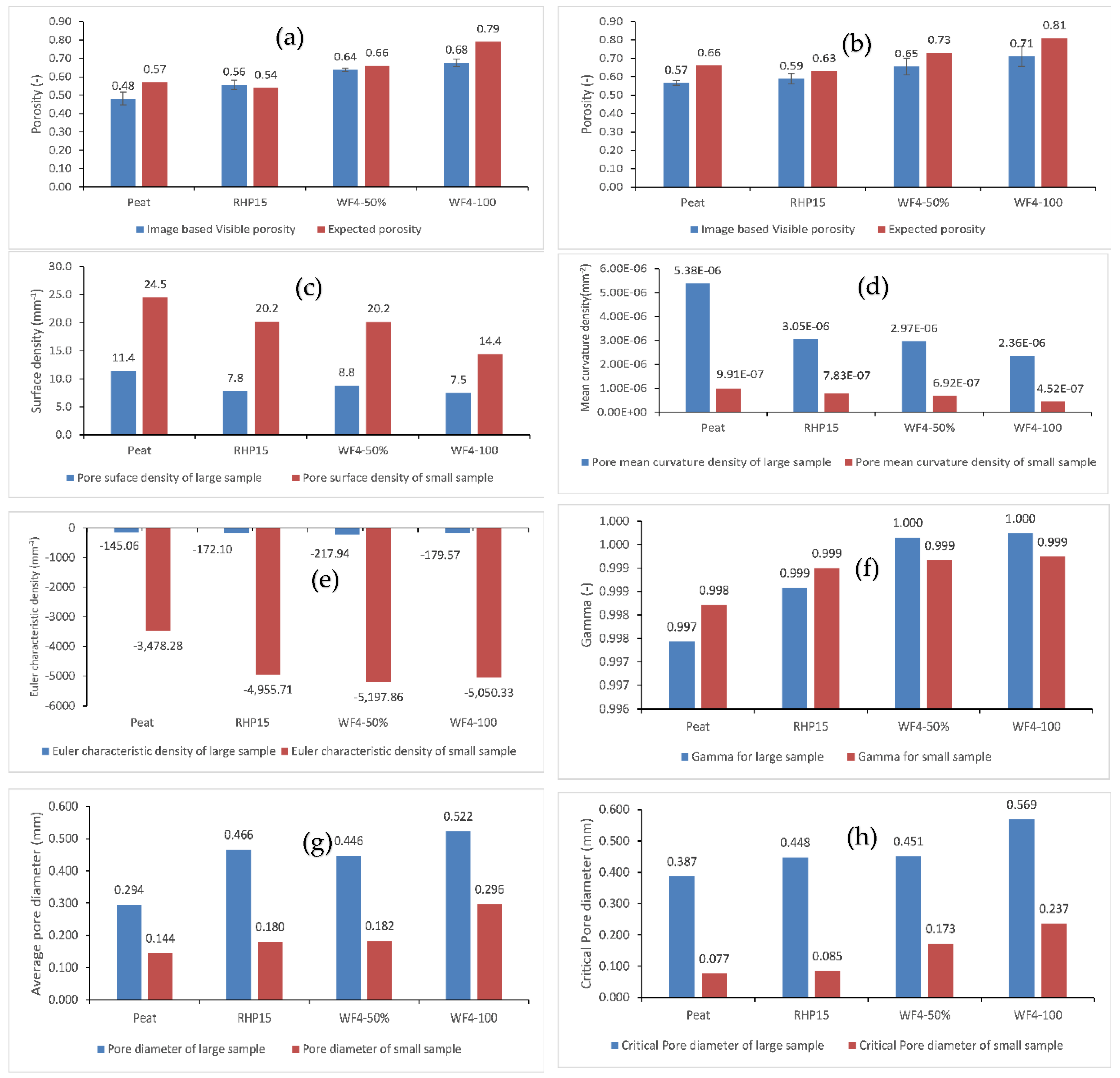
Figure 1. Holographic view of two(a) and three-dimensional (b) divisions, dividing the main images into subvolumes.
Preprints 178902 g001
Figure 2. A flowchart showing image processing for pore structure using Python libraries.
Preprints 178902 g002
Figure 3. A flowchart showing image processing for the pore network model using Python libraries.
Preprints 178902 g003
Figure 4. Determination of REV based on porosity variability across the subvolumes for three-dimensionally divided large images. a: Peat, b: RHP15, c: WF4-50, d: WF4-100. Black bars denote standard deviation.
Preprints 178902 g004
Figure 5. Determination of REV based on visible porosity variability across the subvolumes for two-dimensionally divided large images. a: Peat, b: RHP15, c: WF4-50, d: WF4-100. Black bars denote standard deviation.
Preprints 178902 g005
Figure 6. Determination of REV based on porosity variability across the subvolumes for three-dimensionally divided small images. a: Peat, b: RHP15, c: WF4-50, d: WF4-100. Black bars denote standard deviation.
Preprints 178902 g006aPreprints 178902 g006b
Figure 7. Determination of REV based on visible porosity variability across the subvolumes for two-dimensionally divided small images. a: Peat, b: RHP15, c: WF4-50, d: WF4-100. Black bars denote standard deviation.
Preprints 178902 g007
Figure 8. Pore topological and morphological measures of the studied materials. a and b: image visual porosity and lab-based expected porosity for the large and small samples, respectively; c: pore surface density, d: pore mean curvature density, e: Euler characteristic density, f: Gamma value, g: mean pore diameter, h: critical pore diameter.
Preprints 178902 g008
Figure 9. Comparison between the image-based WRCs and laboratory-based WRCs.
Preprints 178902 g009
Figure 10. Estimation of saturated hydraulic conductivity with PNM simulation, compared to the laboratory measured data.
Preprints 178902 g010
Table 1. Basic physical and chemical properties of the growing media.
Substrate pH EC Organic matter Particle density MWD* Pore#break#
volume
Bulk density Ksat **
- [dS.m-1] [%mas] [g.cm-3] [mm] [cm3.cm-3] [g.cm-3] [cm.s-1]
Peat 3.2 0.05 96.40 1.57 1.18 0.935 0.101 0.0406
RHP15 5.9 0.29 65.09 1.81 4.93 0.924 0.137 0.0447
WF4-50 3.9 0.13 98.03 1.66 1.19 0.925 0.104 0.2286
WF4-100 4.3 0.16 99.40 1.55 1.30 0.942 0.091 0.5624
*: Mean weighted diameter of the particles; **:saturated hydraulic conductivity.
Table 2. Applied manual thresholding for large and small images (pixel values 0-254).
Samples Peat RHP15 WF4-50 WF4-100
Large sample 75 55 80 85
Small sample 85 53 95 110
Table 3. REV derived from large and small images by two criteria (sREV: CV<0.1) and dREV.
Criteria Peat RHP15 WF4-50 WF4-100
Large samples 3D division in µm
sREV (CV<0.1) - 30000 - => 8000
dREV 9000 - 13000 9000 - 13000 10000 - 16000 8000 – 10000
Both criteria fulfilled no no no yes
REV - - - 10000
Large samples 2D division in µm
sRev (CV<0.1) => 2000 => 2000 => 2000 => 2000
dREV 13000 – 21000 13000 – 21000 13000 – 21000 13000 – 21000
Both criteria fulfilled yes yes yes Yes
REV 21000 21000 21000 21000
Small samples 3D division in µm
sRev (CV<0.1) - 9000 4000 4000
dREV 4000 – 9000 3000 – 4000 3000 – 6000 2000 – 3000
Both criteria fulfilled no no yes no
REV - - 4000 -
Small samples 2D division in µm
sRev (CV<0.1) => 500 => 3000 => 500 => 500
dREV 3000 – 6000 3000 – 6000 3000 – 6000 3000 – 6000
Both criteria fulfilled yes yes yes Yes
REV 6000 6000 6000 6000
Disclaimer/Publisher’s Note: The statements, opinions and data contained in all publications are solely those of the individual author(s) and contributor(s) and not of MDPI and/or the editor(s). MDPI and/or the editor(s) disclaim responsibility for any injury to people or property resulting from any ideas, methods, instructions or products referred to in the content.
Copyright: This open access article is published under a Creative Commons CC BY 4.0 license, which permit the free download, distribution, and reuse, provided that the author and preprint are cited in any reuse.
Prerpints.org logo

Preprints.org is a free preprint server supported by MDPI in Basel, Switzerland.

Subscribe

Disclaimer

Terms of Use

Privacy Policy

Privacy Settings

© 2025 MDPI (Basel, Switzerland) unless otherwise stated