Submitted:
20 November 2025
Posted:
20 November 2025
You are already at the latest version
Abstract
Self-organization is common in complex systems, especially those in a metastable state at critical tipping points. This article examines the concept of energy storage and sub-regions formation during self-organization pathways within a specific region of interest known as the control volume. Spontaneous self-organization typically occurs in response to events that trigger a need to respond to an imbalance in the rate of entropy production within the control volume. All entropy-producing processes generate anti-work, enabling the creation of storable power and new sub-boundary pat-terns. A new concept, called anti-work (and related anti-power), is introduced to explain the stability of sub-regions. Examples of triggers include exceeding a local warming rate, earthquakes, or uniquely shaped bird flight formations aimed at energy efficiency, or supercooling, which is the primary example studied in this article to illustrate self-organization. The main conclusion is that the product of temperature and entropy density rate production remains constant during an entropy-producing process. Self-organization leads to a new order and new sub-boundaries. The resilience of this new order is examined in the context of energy partitioning and sub-boundary formation rates. It is observed that self-organization often follows sigmoidal (S-curve) patterns when selecting process pathways. This feature enables the maximization of entropy generation rate and the corresponding availability anti-power. This seemingly universal mechanism for pathway selection in entropy-producing transformations is closely related to the main findings of this article, namely the maximization of the entropy generation rate coupled with energy storage, which helps establish connections across discrete events.
Keywords:
complexity
; entropy production
; solidification
; analogs
; multiscale patterns
; atmosphere
; bird flight
; system boundaries
; utility
; fragility
; efficiency
; anti-work
; resilience
; fractal dimensions
; robustness
; oscillatory behavior
; energy conservation
; S-Curve behavior
; energy storage
; sub-regions and sub-boundaries
1. Introduction
Self-organization in both living and non-living complex systems arises from internal communication, adaptation, and interactions among their components. Complex systems that self-organize dynamically can spontaneously generate new order and new sub-boundaries, while also exhibiting unusual features within these boundaries. In this article, we examine self-organized pathway choices from the perspective of entropy generation rate and the relevant work events that comprise these pathways. The primary objective of this article is to investigate whether the specific process paths selected for self-organization are predictable and whether they enhance the resilience of the self-organized structure.
During self-organization, the central system (control volume) can change its internal patterns in response to one or more triggers, internal or external. These triggers disrupt a metastable state, leading to a new metastable or equilibrium state. Self-organizing systems are also resilient [1,2,3,4,5,6,7,8,9,10,11,12,13,14,15,16,17,18,19,20,21,22,23,24,25,26,27,28,29,30,31,32,33,34,35,36,37,38,39,40,41,42,43,44,45,46,47,48,49,50,51,52,53,54,55,56,57,58,59,60,61,62,63,64,65,66,67,68,69,70,71,72,73,74,75,76,77,78,79,80,81,82,83,84,85,86,87,88,89,90,91,92,93,94,95,96,97,98,99,100,101,102,103,104,105,106,107,108,109,110,111,112,113,114,115,116,117,118,119,120,121,122,123,124,125,126,127,128,129,130,131,132,133,134,135,136,137,138,139,140,141,142]. A key aspect of self-organization is the development or reorganization of new patterns and internal boundaries [3,6,22,44]. The article also investigates, within the limited context of condensed matter, whether self-organized structures form more adaptable and durable arrangements with the new order. While the usefulness of self-organization is not always apparent, experimental evidence suggests that patterns (a hallmark of self-organization) may be linked to more efficient power management during steady-state conditions. The spontaneous formation of a new order in natural and physical systems often involves more efficient resource use [2,3,4,5,6,7,8,9,10,25,26,27,28,29,30,122]. These internal processes involve fundamental changes within a system, sometimes through energy storage at sub-boundaries and in the available work potential from the emerging new order [2,3,44,45,53,54,55,56,57,58,59,60,61,62,63,64,65,66,67,68,69,70,71,72,73,74,75,76,77,78,79,80,81,82,83,84,85,86,87]. In this article, we examine self-organized transformation pathways that are both internally driven, such as supercooled droplet recalescence or sintering, and externally driven, including changes in steady-state solidification velocity and the morphological flow of a liquid in a pipe, where a pressure gradient drives the flow.
Figure 1 illustrates examples of ordering at different scales, showing the sub-boundary regions and their sizes across various levels of repetitive order [44,52,70,74]. Most spontaneous transformations (self-organizing systems) are driven by a force that results from the potential to reduce the system’s free energy within its control volume. However, all real processes must follow a pathway (e.g., a change in temperature over time) to reach a final state, which requires additional energy and a minimum rate of energy availability to overcome the demands of irreversibility during transformation [3,9,14,18,43]. A system that can spontaneously transform finds itself in a metastable or unstable state, requiring a specific rate of entropy production, which can only be met by choosing a process pathway that satisfies this demand. Examples include nucleation and growth pathways that overcome surface energy during the cooling of a liquid into a solid [47,48,49], as well as tropospheric entropy demands for weather prediction [44,45,46]. The significance of the entropy generation rate is one of the key concepts developed by Onsager [40]. Typically, the new order formed after self-organization displays a high level of symmetry (more order). However, the boundaries between self-similar, orderly sub-regions can be less symmetrical (less ordered or even disordered). Symmetrical laws govern the universe, but a system’s actual state may not be symmetrical. This phenomenon, known as "spontaneous symmetry breaking," produces complex and unusual ordered structures. An increase in apparent order can occur when large amounts of energy are released, thereby increasing the surrounding environment’s disorder (entropy). A perfect crystal exemplifies a highly ordered, highly symmetrical system where atoms are arranged in precise, repeating patterns. When the crystal melts, the atoms move randomly, and the liquid phase exhibits much less symmetry and is more disordered. In chemical processes, reaching equilibrium is often associated with an increase in entropy (disorder) and a decrease in symmetry.
The article examines condensed systems used to describe self-organization from a metastable state, employing a control-volume approach [52]. This volume interacts with its surroundings (exterior). In most of the examples chosen for this article, the overall volume changes are minimal, typically reflecting the inverse of the density difference between phases or regions with different symmetries in the initial and final states of a transformation in condensed matter. The textbooks on solidification, which provide additional context on the physical and atomic processes involved in both equilibrium and non-equilibrium solidification, as well as the critical non-equilibrium defects mentioned in the article, are listed in references [47,48,49]. Some earlier concepts from references [4,5,52] are expanded to strengthen the connections between microstates in the energy distribution and larger morphological features resulting from pathway selection during self-organization, using relative entropy (Kullback–Leibler divergence). Key discussions on the implications of this theorem are found in references [19,34]. The article cites published literature on solidification [47,48,49,131,132] and other transformations to validate experimental measurements and property trends, and to support the thermodynamic groupings discussed here for self-organized behavior [4,5,6,44,46,47,48,49,50,51,52,53,54,55,56,57,58,59,60,61,62,63,64,65,66,67,68,69,70,71,72,73,74,75,76,77,78,79,80,81,82,83,84,85,86,87,88,89,90,91,92,93,94,95,96,97,98,99,100,101,102,103,104,105,106,107,108,109,110,111,112,113,114,115,116,117,118,119,120,121,122,123,124,125,126,127,128,129,130,131,132,133,134,135,136,137,138,139].
The article is organized as follows: (1) An introduction to patterns and self-organization, highlighting self-repeating morphologies and resilience; (2) Insights into irreversible processes, work, and the entropy generation rate in classical thermodynamics, with an introduction to anti-work; (3) Validation of MEPR (maximum entropy production rate) for self-organization, entropy generation, and boundary defects; (4) Ease of calculation using the MEPR condition for both steady-state and non-steady-state self-organization; (5) Sub-boundary regions versus sub-regions for energy storage: Fluid Eddies, Solidification, Microstructure, and Particle Sintering Behavior; (6) The importance of sigmoidal-shaped curves (S-curves) in self-organization, followed by (7) a summary and conclusion discussing the significance of S-curves in complex self-organization.
1.1. Self-Repeating Morphologies
Several complex objects possess both resilience and the ability to self-generate dynamically. These are called fractal objects or self-similar patterns. They often appear rough or diffuse, like coastlines. A similar roughness can also be observed in the interfaces of solid-liquid transformations and plasma-treated surfaces [52]. Objects are rarely perfectly linear, smooth, or free of flaws, a fact that becomes more noticeable at specific observation scales than others [17,65,66,67,68]. Fractal objects enable the optimization of features at scales smaller than the observation scale [22,44,52]. In this article, we examine the conditions that lead to varying rates of sub-boundary creation. For all practical purposes, fractal dimensions are considered pathways that generate entropy. Fractal numbers associated with a pathway are thought to be linked to its entropy production rates. Consequently, utility and resilience are interconnected properties when examined at various scales, with utility primarily involving integer powers and resilience sometimes involving non-integer powers. Self-repeating shapes, often called fractals, emerge or become visible through a process of self-organization. These patterns also appear in reaction-diffusion systems, where two or more components interact to create patterns [46,47,48,49,50,51,52,53,54,55,56,57,58,59,60,61,62,63,64,65,66,67,68,69,70,71,72,122]. Many of these patterns can be simulated by repeatedly applying simple rules, as in computer-generated fractal shapes such as the well-known Sierpinski triangles. In nature, these patterns result from efficient, repetitive processes, such as branching in trees, lightning, blood vessel formation, wave-like formations in chaotic systems, star formation, and even at the molecular level with enzymes [20,22,25,50,51,72,77,78]. These examples highlight similarities across different sizes and time scales, as well as in oscillatory conditions, across various fields where they are relevant. Self-similar systems and their associated organized behaviors are understood to be common across different areas of study [139]. This aspect is explored in more detail in Section 6. The exponent of a fundamental unit, such as length, raised to a non-integer power, indicates fractal measurements. Nonetheless, self-similar patterns can be observed across different magnifications (length scales), often repeating within a control volume and in detailed structures at smaller scales. Such structures may not have standard topological dimensions. Fractal dimensions and entropy are related [68,72], often connected morphologically by measurable features such as the area of a grain boundary [73], which we have described as a critical feature in certain types of self-organized systems. Fractal dimension provides a scale-independent measure of a fractal’s complexity. This is also true for the entropy rate density [62].
In this article, we assume that fractal and entropy-producing diffuse interfaces (and sub-boundaries) are essentially different descriptions of the same structure within a complex system spanning multiple volumes and part of a larger system. However, mathematically, fractals are not differentiable [65]. This creates a challenge when applying fractal-based models of self-organization transformation, unlike models that consider the entropy density generation rate (see Figure 1). For physical systems, the units used to describe fractals require normalizing the entropy generation rate per unit volume. Still, it is widely accepted that complex systems can produce entropy at different scales, likely at varying rates depending on the driving conditions of self-organization [1,2,3,4,5,6,7,8,9,10,11,12,13,14,15,16,17,18,19,20,21,22,23,24,25,26,27,28,29,30,31,32,33,34,35,36,37,38,39,40,41,42,43,44]. For example, clouds are estimated to have a fractal dimension of about 2.2; however, this does not provide a method for analyzing their dynamic behavior in rainfall prediction. Conversely, an approach that connects the rate of entropy generation by treating the cloud as a diffuse interface allows for the description of climate events influenced by global warming [44]. It is also important to note that fractal descriptions are not limited to static geometric patterns; they can also depict processes that occur over time (67). Fractal-shaped structures tend to evolve to maximize their surface area for energy or nutrient exchange, as seen in the branching structures of trees [65,67]. When viewed as diffuse interfaces, the conditions required to describe multibranch dendritic shapes or highly fine cellular patterns appear to be those in which the highest rates of entropy generation per unit volume are associated with significant reorganizations at very fine scales [52].
An increase in fractal dimension signifies more complex structures, such as additional dendritic branches or hierarchical formations. The same is true for dendrites. In terms of entropy generation rate, finer dendrites are associated with a higher rate. However, suppose the demand for entropy generation rate per unit continues to grow. In that case, morphology can evolve from finely spaced cells to a high-defect plane front, and eventually into a glassy state. This is shown in [52], where a plot of the entropy generation rate per unit volume against the scale of dominant characteristic events illustrates how entropy generation shifts to smaller volumes of characteristic pattern repeatability. When the coefficient of friction is a key property for wear optimization, both references [52,69] demonstrate a non-linear relationship between the ratio of roughness and a measure of self-similar wave behavior. Non-dimensional properties, such as the coefficient of friction, relate to ratios like (Roughness/Auto Correlation Lengths), which are independent of scale [69].
The article explores the maximum entropy production rate (MEPR) postulate to analyze the pathways leading to self-similar regions within a volume where self-organization occurs. During liquid-to-solid transformations, the solidified boundaries—forming boundaries between similar regions (usually on the millimeter scale)—are high-entropy regions during the self-organization process (3). However, as shown in Section 4, different pathways can be followed to create a high-hardness lattice region or sub-boundary regions, depending on where energy is dissipated. Both pathways result in improved resilience, as discussed below for dislocation movement and crack propagation.
Several researchers now consider the maximum entropy generation rate as the pathway to spontaneous self-organization [4,6,11,12,13,40,41,47,49,50,51,52,53,54,55,62]. At the microscopic level, for atomic- or molecular-scale organization, the key features of the self-organizing region, such as during solidification (Figure 1) or rapid enthalpy-producing metastable oscillatory reactions (Figure 2), involve dynamic activity at the nanoscale that influences properties measurable at larger scales [46,47,48,50,51,70,74].
Figure 1 illustrates self-similar structures in frozen solids containing nano-crystalline icosahedral phases and rain-cloud-forming clusters. These are examples of regions and boundaries that exhibit self-similarity. Figures 1(a, b, and c) display different boundaries and scales of self-similar structures at various magnifications for a solidified Cu-Sn alloy. Figures 1(d) and 1 (e) depict grainy patterns of visibly recognizable diffuse interfaces in evolving thunderclouds on a hot afternoon in Cincinnati, OH, USA (see Section 3 for more details). Occasionally, in condensed matter, boundaries may involve glassy (non-crystalline) phases, even within a crystalline or quasi-crystalline matrix (70). A key characteristic of the internal patterns displayed by a dynamic, self-organized system at steady state is its ability to store energy and entropy in a new pattern [5,52].
Repetitive oscillatory structures, such as the Belousov-Zhabotinsky (B-Z) patterns shown in Figure 2 (a-d), form repetitive patterns (bands with distinct colors and features). These bands are visible in animals such as zebras (Figure 2(a)), which exhibit a banded structure with contrasting colors that repeat at the centimeter scale. Such macro-bands appear alongside non-banded hair follicle growth that remains consistent regardless of the band color. Figures 2(b) and 2(c) depict micro- and nanoscale structures in BZ oscillating systems [50,51,64], illustrating oscillatory reactions in complex systems. These bands [50,51] also correlate with X-ray observations and thermal oscillations, which are hallmark features of classic BZ reactions. Such reactions follow an irreversible path through multiple self-organizing, oscillatory quasi-steady states before completion. Figures 2(d and e) show fatigue serrations related to crack growth and deflection rates [79]. These images show striations caused by fatigue cracks in titanium alloy samples with similar hardness but markedly different fatigue resistance, due to differences in the microstructural size of Widmanstätten colonies [79]. The finer spacings indicate a slower crack growth rate during fatigue crack propagation, resulting in a longer fatigue life. The utility and spacing of zebra stripes, or their branching patterns, are complex to model accurately; however, their main features allow for similar pathway assessments as discussed in this article. Beauty and elegance are also connected to patterns [17,83,87]. The structures of self-organized patterns may serve multiple functions, not all of which are immediately apparent. For example, Zebra stripes are believed to serve as individual signatures for identification, and as discussed in detail in this article, the formation flying of large migratory birds.
For a dynamic, local steady state, unlike a macroscopic static equilibrium, patterns do not need to be spherically symmetrical or isotropic [5]. Bacterial colonies and fluid boundaries exemplify systems that utilize energy to generate collective motion and patterns, similar to those observed in solidified structures [52,53]. When subjected to physical constraints, strong self-localized structures form through processes such as self-replication [50,54,55,64]. Three types of spontaneous, self-organized control scenarios can be identified in self-organizing systems, as shown in Figure 3. Figure 3(a) displays the time-temperature plot for a cooling liquid, which may or may not exhibit metastable states as it cools from a higher temperature to the external reservoir temperature. These include: (1) the system moving toward a thermodynamic equilibrium after a self-organizing event (path A, B, or C); (2) reaching a new steady state or metastable equilibrium (path C) (Section 3) and remaining there; and (3) an oscillatory system that alternates between states while decaying very slowly (Figure 2). The first two are well exemplified by crystallization (crystal growth) either by cooling [46,47,48,49,76] or Rapid Pressurization [75,138], A liquid droplet can be cooled from a high temperature and solidified into a powder (a non-steady-state process), or a crystal can be grown using the Czochralski (CZ) method by pulling a liquid into a cooler region under steady conditions. Both techniques are essential in physical manufacturing from an engineering perspective. They involve complex, multicomponent, multiphase alloy transformations, resulting in a new, functionally useful repetitive scale with utility tied to a specific length. The third type is easily visualized in low- and high-temperature Belousov–Zhabotinsky reactions, which also influence the development of new high-temperature alloys [50,51].
1.2. Utility and Resilience
Self-organization leads to order and resilience (which has a contextual meaning). Resilience can be defined in various ways, as discussed below, and its meaning can differ across scales of understanding. In this article, we examine resilience at various scales that can result from self-organization and relate it to the energy processes underlying self-organization.
Resilience is a property that enables disturbances to be dampened, meaning they are not amplified. Turbulent flows are often described as "resilient" (or more commonly, "stable" or "robust" once established) because of their inherent ability to rapidly dissipate disturbances and maintain their overall chaotic, mixed state through internal mechanisms. It can be argued that properties such as the hardness of an alloy [43,44,47,48,49,50,69,70,74,75,76,77,78,79,80,81,82,83,84,85,86,87,131,132] reflect aspects of its usefulness, a term enabled by resilience. A material’s stress intensity factor for resisting spontaneous crack growth [70,79,132] or wear [52,69,70,74,131,132] could serve as a measure of its resilience. However, it is noteworthy that hardness also indicates resistance to dislocation movements at sub-boundaries or by precipitates, so both hardness and fracture resistance could be somewhat synonymous at different scales of measurement, but not necessarily so, except under certain conditions. Hardness of the lattice (the sub-regions) could result from Peierls stress for lattice dislocations, which represents the fundamental measure of the intrinsic lattice resistance to dislocation motion. Its value is unique to each material, depending on its crystal structure and bonding characteristics. Resistance to crack growth may be inversely related to lattice hardness unless sub-boundary regions become involved. Often, resistance to degradation or external stress must overcome the periodic potential of organized patterns, such as lattices or nano-precipitates within the lattice or at sub-boundaries [85,86]. Hardness is measured in Joules per cubic meter (J/m³) and depends on grain or dendrite size [47,48,49]. Sometimes, hardness is also expressed in terms of lattice friction and a Hall-Petch constant with units of J/m2. Fracture toughness, which indicates a material’s resistance to crack growth, is measured in J/m2 (80). These measures describe the resistance to dislocations or cracks moving smoothly across periodically varying potential barriers. However, fracture resistance is also expressed as energy per unit area, similar to hardness. Peierls stress, which resists dislocation movement, is measured in Pa (N/m²) or sometimes as a non-dimensional number when divided by the shear modulus. A material with low Peierls stress, facilitating easier dislocation motion, is generally better at blunting cracks and thus more resilient or tougher. Conversely, high Peierls stress, as seen in ceramics, resists dislocation motion, making such materials more brittle and less tough. The specific wear rate has units of m³/J (chalk: 10^-12 m²/N to diamond: 10^-19 m²/N) [69]. Graded or inhomogeneous materials and properties, such as viscoelasticity, involve non-integer powers of material properties. The fracture toughness can change with orientation in brittle materials, whereas the hardness remains essentially isotropic when measured on large quasi-crystals with oriented sub-boundaries [124,131,132]. The phenomenon of material creep occurs when a system deforms under its own weight or under anisotropic loads, typically at high temperatures, close to but below its melting point or the point of bond breakage. Here, having many boundaries increases the creep rate (strain rate), whereas fracture toughness decreases. Creep, unlike resistance to dislocations or cracks, could be an event that requires resilience during a self-organizing process (i.e., continuous feedback mechanisms are active). During creep, grain boundaries slide past each other, and in some cases, they may migrate toward planes of maximum shear stress, changing the orientation of grains and grain boundaries. This reorientation is a key part of the deformation process and can also involve the movement of dislocations and vacancies. This unusual phenomenon is discussed in Sections 4 and 5, as well as in references [18,47,48,130,131,132].
We thus recognize that resilience is a term associated with the system’s ability (or resistance) to energy, i.e., the energy required per unit volume or area, and that a more resilient material will be able to overcome a more energetic disturbance. Both heat- and work-based degradation can weaken the defenses of a periodic, ordered barrier in a similar manner, whether for an army facing an onslaught of intruders or for opposition on a more microscopic scale to dislocation movement that can cause yielding or growth in a crystalline lattice [70,71,72,73,74,75,76,77,78,79,80,81,82,83,84,85,86].
This article examines the entropy generation rate as a key variable [4,5] in the formation of pathways and sub-boundaries during self-organization. The pathway selection influences the morphological scale of the self-organized pattern (4). In this way, the entropy generation rate is linked to measurable engineering properties, as it affects pattern formation, which in turn impacts these properties [4,47,48,49,79,80,86]. The article uses a classical thermodynamic approach, based on Onsager’s work (18, 40), to address flux entropy generation arising from the irreversible transport of measurable quantities within a system. Irreversible transport refers to phenomena driven by energy, matter, pressure, and charge gradients. Another aspect of irreversible entropy generation is configurational entropy, a component of a system’s total entropy related to the number of possible spatial arrangements, or microstates, of particles and their influence on energy distribution. Its generation involves changes in these arrangements or the creation of new active microstates.
Several published studies highlight the importance of comparing a process to a reversible one in terms of the thermodynamic uncertainty of interactions (in a canonical sense) for self-organizing systems [61,82,83,84]. Physical processes can be described by stochastic models, such as Markov chains and diffusion processes, and entropy production can be defined probabilistically for these models. As seen in many phase-field studies of liquid-to-solid ordering and morphological evolution, changes in an order parameter are used to infer the system’s dynamics. The uncertainty per unit of work output can measure the efficiency of ordering during self-organization [61], relating it to a grouping like [(1/R)(δS(config)/δW)] where T, δS(config), R, and δW stand for temperature, configurational entropy (a form of entropy generation), the universal gas constant, and work, respectively. However, this grouping feels somewhat awkward because the path should ideally be related to a rate, which is difficult in a probabilistic or stochastic model. Nonetheless, predictions [82,83,84] suggest maximum efficiency of ordering at critical temperatures, thus implying a maximal tendency for ordering based on the Gouy-Stodola theorem in reference [81], which states that the rate of exergy destruction (lost work potential) in a thermodynamic process is directly proportional to the rate of entropy generation during that process. Additionally, the maximum entropy generation rate or power requirements for various scales of subregion volumes involved in self-organizing transformations can be modeled by analyzing energy, matter, or configurational entropy fluxes, respectively [4,18,40,52,84].
2. Insights into Irreversible Processes, Work, and the Entropy Generation Rate in Classical Thermodynamic Formulations
No process path is reversible. A system (control volume) can spontaneously transition from one equilibrium (or metastable) state to another, making the process irreversible. A simple example is a hot object that cools spontaneously by releasing energy to the environment (the sink) through an irreversible heat transfer process. Any irreversible process increases the entropy of the universe. The presence of gradients in temperature, chemical potential, or pressure generates a rate of entropy (Ṡgen), making the process path thermodynamically irreversible [18,39,40,41,42,43,71].
Assume that heat flows in a bar with length L, cross-sectional area A, and thermal conductivity κ, placed between two reservoirs T1 and T0 (T1>T0). A linear gradient is established (Figure 3), especially when the temperature difference is small. The heat flow rate, Q̇ (J/s), at steady state is constant. Local equilibrium conditions prevail. The rate of entropy generation in the bar is [33,71]:
This new entropy also flows down the temperature gradient along with the thermal energy in the bar and is delivered to the reservoir at T0 when the steady state is established. Because of a linear temperature gradient, Q̇ can also be written as:
Giving the entropy generation rate as,
The Carnot efficiency limits the maximum work that can be done between two temperatures. The maximum possible power, Pmax, available from a heat engine operating between and for a heat transfer rate is
Thus, although the physical situation in Figure 4(a) is at a steady-state condition, it is an irreversible pathway defined by the local equilibrium conditions (The local equilibrium condition is required for the heat flux to be defined and for an experimentally measurable (verifiable) linear temperature gradient to be established).
Regardless, even for an idealistic heat engine operating between reservoirs and The maximum power output, Pmax (J/s), must include a heat transfer coefficient between the corresponding temperatures of the heat engine, (RE), and (RE), where RE stands for Reversible Engine. Figure 3(b) illustrates a reversible heat engine between two thermal reservoirs, yielding a maximum power (Pmax) that depends on the heat transfer coefficient (J/m² · K ·s) and the contact area (A) with the thermal reservoirs [71].
In the ideal case (i.e., when no entropy is generated)
In the realistic case
Because T0 < T1, Equation (2.7) indicates that a realistic Pmax is always less than the ideal Pmax(ideal), as given in Equation (2.4), for a fixed energy (heat) rate extracted from the hot reservoir. The corresponding entropy generation, which effectively reduces the available power from the ideal Carnot amount, is transferred with the heat to the cold reservoir—that is, an energy rate sent to the cold reservoir exceeds what would have been transferred if no entropy had been generated. In a way, this also reflects the work done on the system to maintain the reversible cycle processes shown in Figure 4(b).
Equation (2.5) represents the maximum entropy generation rate because it is the highest work rate possible, divided by the lowest temperature within the range. Therefore, the rate of entropy production is always at a maximum in a steady-state simple thermal heat transfer process or heat engine. Steady state is generally defined as a condition where local equilibrium exists, regardless of thermodynamic fluxes, temperature, pressure, charge, or chemical potential gradients. In other words, it applies when macroscopic temperature and other thermodynamic properties can be defined and measured. Similar arguments regarding the rate of entropy generation were first presented in references [4,5].
Note that in the example shown in Figure 4, the rod length remains constant. In reality, the rod must expand because of a positive coefficient of expansion, with T0 serving as a reservoir. Therefore, constraining it results in work being done on the system. Energy dissipation is the process through which work and energy convert into forms that can be transferred as heat during a process. It primarily represents an energy loss that occurs through irreversible processes, such as friction, resistance, or other dissipative forces, resulting in a decrease in the system’s mechanical or functional energy over time. However, this dissipation can instead be thought of as anti-work, creating sub-boundaries and therefore being considered anti-work (Sections 3 and 4).
Work can be done on the system due to non-ideality. This permits defining Tav in terms of and , as was done for solidification, where the product (Tav.Ṡgen) is also possibly maximized, as shown in Equation (2.9) below, because the heat transfer coefficient, the energy transfer rate, Q̇̇1, and the temperatures and are fixed in this problem. The loss in work-potential is thus approximated by:
The Maximum (if Q̇1=h.A.T1). Following Figure 5, this condition occurs at a Tav where: , which occurs at the Pmax(ideal) of 0.75. This implies that if entropy is generated at its maximum value (e.g., spontaneous self-reorganization, as discussed in later sections of this article), the maximum work conversion efficiency is only 25%.
The examples discussed above are cases where spontaneous heat flow is obtained, and the work done on the system was external, the rod was fictitiously compressed (an assumption that permits use of the thermal conductivity), or a heat engine operated between two temperatures, and the heat engine was operated by an external energy source. Another way to think about this is to consider two equal masses initially at T1 and To that are brought to equilibrium by physical contact. If they were brought to equilibrium by touching each other (a condition that maximizes entropy generation), then the final temperature would be = (T1 + T0)/2. If on the other hand, they were brought to an equilibrium temperature by transferring heat between them with the help of a device that does work to prevent entropy generation, the equilibrium temperature would be .
Energy dissipation is defined as the process by which useful energy is transformed into a less useful, often unusable form, such as heat. This can increase the entropy at a specific location during a process. It’s commonly known as the type of energy loss that results from irreversible processes, like friction, electrical resistance, or other dissipative forces, which cause a decrease in the system’s useful energy typically mechanical or electrical energy) over time.
Note, however, that in the examples discussed above, no entropy production pathway results in a temperature lower than that of the entropy-producing pathway. This is because the entropy generation pathway leads to a condition where the internal energy is higher at the end of the equilibration process. Therefore, energy dissipated as heat can, in principle, be partially converted into work, albeit only after the original process is completed. L process.
Understanding the work done on the system is crucial for understanding any entropy-producing (generating) system. This anti-work effectively encompasses the energy transferred into the system and is either stored within its high-entropy sub-boundaries or within a low-entropy lattice (subregions). This energy can be utilized beneficially.
The following sections analyze whether the rate of entropy generation reaches its maximum value and the implications of stored energy within sub-region boundaries when no external work is performed (we refer to this as anti-work to distinguish it from external work done on the system). We also explore whether the creation of sub-boundaries results from maximizing anti-work.
3. Validations MEPR (Maximum Entropy Production Rate) for Self-Organization, Entropy Generation Rate, and Boundary Defects: Fluid Eddies, Solidification, Microstructure, and Particle Sintering Behavior
One of the key understandings developed in this article to analyze self-organizational behavior relies heavily on entropy generation rates. A brief analysis of this MEPR is presented in this section. Wherever model results are available and can be compared with experiments and observations, they are presented. In addition, Turbulence, Sintering, and Recrystallization are also examined, although no calculations are provided for these processes to facilitate experimental and modeling comparisons. A connection between a macroscopic principle and the microscopic features of self-organizing systems is established by applying the MEPR (Maximum Entropy Production Rate) principle, first outlined in the Gouy-Stodola theorem (see Section 1 above). It has been previously argued and discussed in detail in the introduction of this article that pathways that maximize the entropy generation rate provide a basis for explaining the complex, ordered patterns that can spontaneously emerge in non-equilibrium systems. While reducing entropy production (generation) rate to zero is necessary to reach classical thermodynamic equilibrium in a closed system, Sekhar [4] has demonstrated, through morphological examples, that increasing the rate of entropy production (generation) to its maximum within an open control volume is a valid way to describe the shape and other defect evolutionary features in a steady-state transformation. Shape formation and its relation to entropy generation rates have also been explored by Martyushev [6] and Hill [38], among others, with physical examples drawn from various fields. Non-steady state systems are discussed later in this article.
According to MEPR, a system’s internal structure will evolve toward a state that maximizes its entropy generation rate (Ṡgen). The straightforward proof of MEPR presented in Section 2 above may not demonstrate that the MEPR hypothesis always holds. Regardless, the MEPR formulation has been successfully tested in more complex situations (Table 1). Bensah et al. [23] have shown that the entropy maximization rate is a fundamental principle that describes transitions between microstructural morphologies, such as self-organized dendrites, cells, or grains that develop during solidification, and that it effectively predicts physical constants [23,52,62]. Some of these measurements and calculations are shown in Table 1. Experimentally recorded and calculated bird flight angles with the MEPR formulation are matched [5] as shown in Table 1 and Table 2.
In entropy-generation-rate models, a diffuse-interface approach has proven helpful for accurately capturing morphological transitions [4,23,44]. A diffuse interface represents a boundary between two different phases or materials that is not necessarily sharp. The key features of a diffuse interface include a finite thickness, a smooth transition of the order parameter or transformed fraction, and a somewhat unclear mixing of phases that are not easily visualized, even in clouds. There are a few clear images of diffuse interfaces; however, within the diffuse interface, the phases may not be strictly separated but somewhat mixed, which better reflects physical phenomena at a microscopic level. The reaction occurring at the diffuse interface is a mixed-order reaction [4].
With MEPR, explicit modeling of the role of boundary defects in driving entropy generation can be addressed. This involves mathematically accounting for the work and energy required to form new interfaces, such as those that form during solidification or wear [52]. MEPR incorporates terms that quantify the contributions of defects to the total entropy generation. These include the work rate (dW/dt) and defect entropy, which were introduced in the previous section as antiwork, a key process of self-organization. In reference [4], this is described as (ωD/Tav), where ωD is the defect energy and Tav, as described in Section 2, is the average temperature at which the loss in efficiency is maximized. This term, along with an entropy term associated with chemical species segregation and two-phase mixing at the boundaries, contributes to the overall entropy generated.
Cloud formations and energy distribution between various weather phenomena are accurately determined with MEPR [44]. The cloud cluster photograph (Figure 1d) was taken with an iPhone® 12 through a colored window on a cloudy Saturday afternoon, August 23, 2025, at 2:10 pm. The sun is directly overhead, and a diffuse interface [44] exists between the dark and light regions within the clear sky. The camera captures blue and yellow hues, as well as dark, high-water-content regions. Despite the temperature being 28°C and the relative humidity being 54%, it did not rain. This is inferred due to the development of many clouds that formed horizontally rather than vertically (Figure 1(e)). The horizontal development (spreading instead of vertical growth) relates to a low entropy rate change [44]. MEPR has been used to predict large-scale weather patterns [1,44,45,46]. It provides a useful conceptual and methodological tool for understanding the macro-scale thermodynamic forces driving thunderstorm activity. It can assist in developing more reliable parameterizations for convective processes in large-scale climate models. MEPR has also been used to analyze the behavior of both equilibrium and non-equilibrium clouds. Interactions between high-velocity winds and significant water-containing clouds can lead to the formation of multicellular thunderstorms. Lightning can also transfer entropy out of a cloud, increasing the demand for entropy generation per unit time. For non-equilibrium thunderstorm cumulonimbus clouds with the current tropospheric expansion rate, the upward velocity of thunderclouds, V(m/s), is related in the MEPR model [44] to the cloud thickness, and a constant Z ~0.05 (s-1).
Vc3 ~ Z.xc
The maximum entropy production rate hypothesis is the only solidification model that has accurately predicted bifurcations and high-temperature liquid diffusion constants [4,23,62,63], which are consistent with experimental data. MEPR models the energy needed to create and sustain morphological features as a work rate and includes additional terms for the entropic contribution of defects. Similarly, it has been able to explain the lower friction coefficient resulting from self-organization during pairwise friction at the Hertzian regions between metallic contacts [52]. The importance of sub-boundary defects in driving entropy generation has been key in validating models of entropy generation rate. This involves mathematically accounting for the work and energy involved in forming new interfaces, such as during solidification or wear. The MEPR maximization principle avoids the fine-tuning required in kinetic models with arbitrary order parameters, as the energy flow naturally aligns with efficiency goals. This is also demonstrated for heat engines (Section 2). Because it provides an additional maximization condition, MEPR also enables seamless connections across different pattern scales.
Birds such as Canadian geese (Branta canadensis) display several closely related flight pattern formations during the steady-state part of their long migratory flights (5). A V-shaped formation is often observed during high-altitude long flights, as shown in Figure 1. The observed “V” formation during the long-distance migration of large birds is related to MEPR [5]. The “V” formation is compared to other closely related but distinctly different formations that a flock can also adopt.
A thermodynamic model of bird flight formations shows that efficient thermal herding is achievable by flying in specific formations [5]. The analysis of the model’s results indicates that the “V” formation (referred to as the SV formation) is the pattern that optimizes energy use for the flight duration. Comparing it with experimental data indicates that the MEPR thermodynamic model provides reasonable predictions. The MEPR postulate for bird flight formation predicts the emergence of the most optimal self-organized formation, the "V" formation, which is also commonly observed. The model verifies three main experimental findings: (i) the preference for a V formation over other formations, (ii) the energy-saving benefits of flying in the V formation, and (iii) the decrease in energy use as flock size grows. See Figure 6. Additionally, the "V" formation allows for slight adjustments to accommodate birds of different sizes by offering enough lateral movement. When creating a pattern with the highest rate of entropy generation or the highest rate per unit of energy, a migrating flock organizes into its most energy-efficient and stable pattern.
The V and other closely related formations allow spatial separation, enabling optimal bird temperature during the flight passage. This formation also ensures that all trailing birds experience the same thermal environment. As flock size increases, the power expended per bird decreases when comparing the same velocity or mass flow rate. Compared to flying alone, flock formation reduces fatigue for each bird, allowing the flock to cover larger distances [5].
The angle for the V depends on the bird’s dimensions in the pattern, assuming all birds are the same size. Table 2 lists the reported size variations for Canada Geese [105,106,107]. The V angle predicted by the model is 113-116 degrees, calculated as 2 × tan^-1 (Wingspan/Length) for optimized flight formations. This angle aligns well with the reported angles for small flocks [105,106,107], although some variation is expected due to differences in goose sizes. The results for the reasons for formation flying, based on the thermodynamic model with MEPR conditions, indicate a very high probability of a physical basis for formation flying, in addition to the "behavior only" preferences sometimes reported in the ornithological literature. It should be noted that there are reports that suggest that almost forty-one bird species that fly long migratory routes do so often with V-type formations (5), which could indicate that thermal herding is essential for flight optimization. Note that the V formation is a way that no new boundaries between birds must form while maximizing the entropy production rate (Figure 6 (a) and (b)). This implies that the anti-work or energy gained from formation flying can be fully utilized for additional power whenever needed.
As the flock size increases, the distribution of bird sizes may need to be fitted to the formation. A distribution of wingspans will change the birds’ leg separation, but not affect any thermal calculations, because the model assumes energy transfer only along the flight direction. A decrease in the overall median length/wingspan ratio will lead to a sharper V angle. This suggests the MEPR-based angle prediction of 113°-116° is a reasonable estimate for the higher V angles in large Canada Geese. Angles above those predicted are mostly seen only in very small flocks [5,105,106], where there is likely a greater need for behavior and visual conformity, with less emphasis on energy optimization from flock size (since ostensibly small flocks can coordinate more easily for frequent stops). Sharper angles may also occur in the thermodynamic model if the birds are not closely aligned in the flight direction, as reported in reference [107], or if a slight variation to the V shape is chosen (several of which are described in Reference [5].
For completeness, it should be noted that a well-defined organizational phenomenon is also observed in ball bearings that are organized in an orderly manner in a rotational system, subject to vibration, at high angular speeds [141]. The symmetrical resting positions of ball bearings are governed by conservation of angular momentum and by the force balance that promotes well-defined organization (such as the stability of bird formations in flight [5]) or even the patterns observed in vibrating plates [142]. Waves lose energy from friction or turbulence. The organized behavior associated with standing waves [142] is observed, despite energy loss over time.
3.1. Minimum Size for Turbulent Eddies and Solidification Morphologies
Although not yet completely understood for several morphological transformations, the limits on particular shapes exist. For steady laminar and turbulent flows, Pal [33] has derived entropy generation rates that depend on fluid properties, velocity, and pipe diameter, assuming constant temperature and negligible temperature dependence. A critical velocity indicates the transition between flow types, where energy is extracted by large eddies that are anisotropic and unaffected by viscosity. In contrast, small eddies are isotropic and driven by viscosity. For steady and fully developed laminar flow and for turbulent flows of a Newtonian liquid in a smooth pipe, the entropy generation rate per unit length of pipe is derived by Pal [33] as:
Laminar Flow:
Ṡgen~(8𝜋/𝑇)𝜇𝑉2
Turbulent Flow:
Ṡgen~(0.079𝜋/2𝑇)𝜇0.25𝜌0.75𝐷0.75𝑉2.75
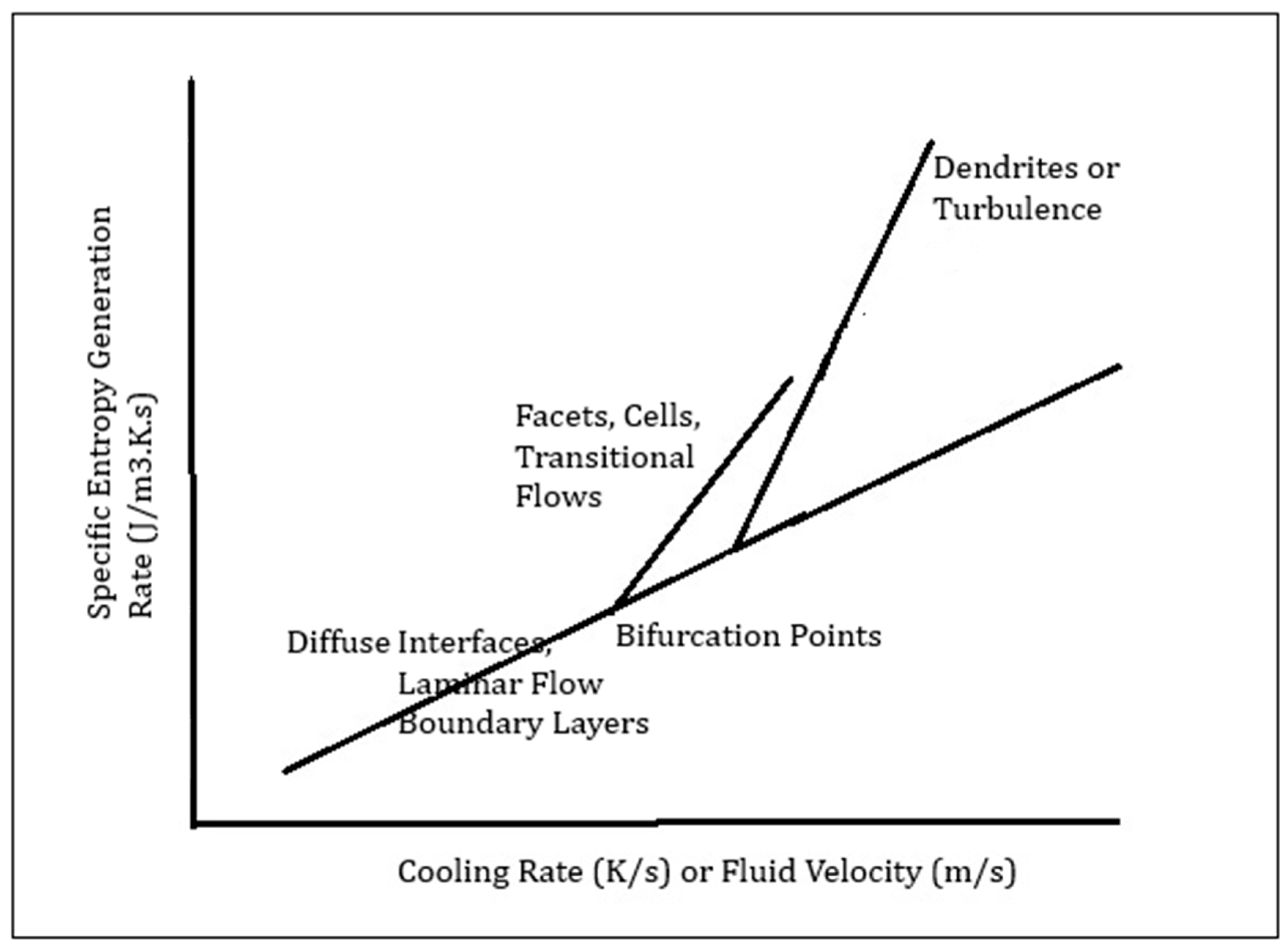
Similar to the known variations in tip radius size of dendrites with the Peclet number [47,48] Equation 3.5, that can be formulated as the diffuse interface size variation with the cooling rate during solidification [61] shown in Figure (6a), the plots of the Reynolds number and entropy generation rate show an increase with flow speed, with the relationship differing between laminar and turbulent regimes (Equations 3.2 and 3.3). In laminar flow, entropy increases linearly with velocity; in turbulence, the increase is steeper, shifting upward with larger pipe diameters. Higher Reynolds numbers indicate more turbulence, a broader eddy spectrum, and greater scale separation, with energy cascading to smaller scales where it dissipates. As the Reynolds number increases, large eddies develop and become dominant. However, the smallest eddies that are particularly viscosity dependent are described by Kolmogorov’s limit [90,91,95].
In both turbulent and laminar flows, the entropy generation rate per unit length of the pipe depends on fluid density (ρ), as well as viscosity (μ) and average fluid velocity (V). T is assumed to be constant in the analysis. Although this assumption isn’t strictly valid in entropy generation analysis, Pal [33] suggests that the temperature dependency may be small for pipe flows. This holds if the eddy diameters have not reached the Kolmogorov scale. Note the dependency on pipe diameter (D) in turbulent flows. There are notable similarities between cellular-to-dendritic transitions during solidification and laminar-to-turbulent flows. A critical velocity exists where morphological transitions occur, with each morphology associated with a characteristic slope of Sġen versus velocity. The largest eddies extract kinetic energy from the mean flow, thereby serving as a source of energy. The length scale is comparable to the flow’s dimensions. These processes are highly anisotropic and are largely unaffected by viscosity. Most transport and mixing happen in this range. The smallest eddies have universal characteristics independent of the flow geometry and conditions. Those eddies in this range usually receive energy from the larger eddies and dissipate their energy into heat through the fluid’s molecular viscosity. These eddies are isotropic, with length scales described by the Kolmogorov scales [90,91,95]. It is assumed that the small-scale eddies are determined by viscosity and dissipation. Eddies in this region can be characterized by the turbulent dissipation ε and the wave number κ (or eddy size L). The energy E = Ckκ-5/3ε2/3 changes with eddy size or curvature and is defined by the constant Ck ~ 1.5 [94] as a function of κ, the curvature of an eddy, where ε is the energy dissipation rate density. However, unlike solidification, the pictorial descriptions of self-organized turbulent flow [91] do not always present a single, universally accepted image [10,91,92,93,94,95]; instead, they offer a conceptual view of turbulence development and organization within a fluid featuring varying eddy sizes. Such diagrams display chaotic, swirling patterns of eddies and currents overlaid on mean flow, contrasting with smooth, laminar flow. Turbulence involves eddies of different sizes; at high Reynolds numbers, a scale separation exists between large and small eddies. Turbulent flow is diffusive, with chaotic eddies enhancing boundary layer momentum transfer, delaying separation, increasing resistance and heat transfer, and dissipating kinetic energy into thermal energy. Following the MEPR condition for minor disturbances, where the viscosity is unchanged by velocity or temperature for Laminar flow (Equation 3.2), indicates that the temperature multiplied rate of velocity disturbance is equal to the rate of change of the fluid’s temperature (which will be lost through the pipe walls). The ratio of the largest to the smallest eddy scale with the Reynolds number [91] in the following manner:
Consequently, it is related to the Sgen rate for turbulent flows via Equation (3.3). Re is the Reynolds number for a Newtonian flow, and L is the largest eddy. The entropy generation rate multiplied by the average temperature, differentiated with respect to a spatial coordinate, can produce shear. Shear serves a dual role: it is a source of turbulence in the system (such as in boundary-layer turbulence), and it also alters the energy transfer from large to small scales by affecting the Kolmogorov limits [90].
The imposed cooling rate during solidification in a positive temperature gradient environment (i.e., dT/dx>0) is similarly related to the entropy generation rate [3,61], thereby ensuring that the Trivedi limit depends on it. Likewise, there is a threshold beyond which cell and dendrite boundaries cease to form, resulting in a planar interface at very high transformation velocities during solidification. Mullins and Sekerka first described the formation of high-velocity planar interfaces [47,48]. This was later recognized as a very wide, diffuse interface [4,23,52].
Both the Kolmogorov scale eddy development discussed above and the tip of a dendrite during solidification impose limits on the morphology within specific domains of entropy generation rate. During solidification, the Trivedi limits apply for the radius of the largest and smallest diameters of the solidification dendrite tip, which is defined by the relationship [47,48,92,93,94].
Rtip/Rtip-min= Pe . (Va/V)
Where Pe is the Peclet number, Va is the absolute velocity at which dissipation reaches its maximum (i.e., boundaries disappear and a broad diffuse phase forms [4,52], similar to the Kolmogorov limit [91,92,93,94]. In viscous dissipation, heat is produced. The morphology of eddies approaching the Kolmogorov limit is not well studied, but some branching and optimized structures for energy dissipation are thought to be possible [94]. The energy dissipates as heat, and rotational inertial work from the overall kinetic energy of turbulent flow is thus converted into heat, boundary work, similar to the potential energy (lattice energy) during solidification. From reference [61], we can relate the cooling rate to the Sgen rate at the critical bifurcation to the cooling rate (V.G), where V is the solidification velocity, G is the temperature gradient, and Nc is a constant that includes diffusivity.
Figure 7.
The rate of entropy generation increases with the driving force (a) Cooling Rate [62] or (b) Pressure drop in a pipe of diameter D from reference [31], with an increase with the driving force, namely cooling rate or velocity (pressure gradient), respectively. Both axes are plotted on a log scale.
The crystallization case has more experimental studies related to the Trivedi limits [89,93,94]. Kolmogorov’s limit suggests that an energy flux exists towards small scales, which eventually leads to the dissipation of kinetic energy [91], , where V is the velocity and m²/s³) is the rate of energy dissipation (m²/s³) [91,92]. However, for fluid flow, an estimate of energy dissipation is only made with difficulty because the energy dissipation occurs with unclear boundary formation information, albeit with some spread in curvature, similar to the spread in dendrite arm sizes shown for secondary dendrite arms in Figure 8.
3.2. Sintering and Densification
Particle sintering [95], in which heating the material or creating a temperature gradient causes the system to lower its overall energy by expanding grain boundaries and reducing porosity, is an entropy-generating process. Differences in chemical potential and interfacial energy across a powder compact generate the thermodynamic driving force for sintering. Areas with convex (positive) curvature have higher chemical potential [96], while concave (negative) curvature areas have lower chemical potential. In a solid compact requiring densification, atoms diffuse from regions of high chemical potential, such as the convex surfaces of powder particles, to regions of low chemical potential, like the concave "necks" between particles. This mass transfer decreases the system’s total surface area and releases energy. The pathway taken can result in different morphological outcomes. For example, sintering may involve grain growth without densification: if the difference between surface and grain boundary energies is small, pores can remain stable. In such cases, the system’s free energy decreases through grain growth, eliminating grain boundaries, rather than pore shrinkage. Conversely, densification can occur without grain growth when the grain boundary energy is much lower than the surface energy. In this scenario, the system reduces its free energy by forming grain boundaries and eliminating pore surfaces, resulting in minimal changes in grain size and leading to rapid densification. The most common scenario involves both densification and grain growth co-occurring: initially, pore elimination dominates, but as surface energy decreases, grain growth becomes the primary mechanism for further reducing free energy. Kinetic factors are influenced by the formation of a neck at grain contacts (96). The reduction in surface energy over time, along with the development of grain boundaries, is like balancing a diffuse interface region with grain or dendrite boundaries [4,61,62]. Ultimately, the tipping point that causes morphological transitions is a response to the requirement to minimize free energy or to an imbalance in entropy generation rate.
During sintering, entropy production involves at least four factors: heat conduction, mass transfer, chemical reactions, and grain-boundary movement [97]. Rapid sintering processes generate enthalpy [50]. Similarly, the high configurational entropy in high entropy alloys can influence sintering behavior, sometimes hindering grain boundary migration [98]. An entropy gradient may exist at grain interfaces, affecting material properties such as Hardness.
Sintering can be effectively slowed down by selecting pathways that prevent the coalescence of expensive catalysts [98]. Therefore, in principle, lower-cost, high-temperature processes [99] can replace costly high-entropy material catalysts. The ratio of grain boundary energy to surface energy () is a key thermodynamic parameter that drives the sintering process. Sintering requires that the formation of grain boundaries is energetically favorable, meaning that. for isolated particles. Sintering additives and the compressive pressure of resistive heating can be used to provide energy assistance, either enhancing or inhibiting the sintering process. Grain growth reduces the total grain boundary area, thereby decreasing the system’s overall free energy. The question is whether MEPR is followed during the sintering process. Does any work done on the system become a requirement? What happens when a current is applied? What occurs when pressure is applied? Since there are always several possibilities and pathways for the objectives of sintering, it is left for a future publication to determine if maximum entropy production applies to every sintering scenario. However, there is no reason to believe it is not.
All real self-driven sintering processes will produce entropy (Sgen) [6,14,26,31,47,51,62,64,97]. Similarly, during Recovery and Recrystallization [131,132,135,136], entropy is generated. The key point is that sintering, grain growth, or even the merging of soap bubbles are physical processes in which boundary areas, such as particle surfaces or grain boundaries, may decrease during spontaneous self-organization. At first glance, this differs from the solidification and turbulence examples discussed earlier, where new boundaries form during pathway selection, helping explain anti-work or work done on a control volume during self-organization. However, the volume reduction during sintering absorbs the anti-work involved in the process. Pathway choices are made for various reasons [5,110] that involve entropy generation and work done inside a control volume. These choices and sub-regions build resilience against deformation, reduce wasteful power expenditure, and act as barriers to prevent epidemics [110]. In some cases, energy release can cause fractures and reorganize boundaries to enhance resilience [111,132,133].
4.0. Ease of Computation with the MEPR Condition for Steady State and Non-Steady State Self-Organization
The MEPR condition discussed above permits kinetic determinations, particularly when morphological transitions are involved. As we will note later, these are important for understanding the stability and resilience of complex structures. Two examples are provided below: one from a steady-state, one-dimensional morphological transition and another from a non-steady-state, nucleation-triggered transformation leading to an ordered organizational process that offers further validation and extensions for understanding the significance of the rate of entropy generation as a possible principle that may apply to several aspects of self-organization.
4.1. Morphological Transition Modeling at Steady State
Morphological models using the MEPR principle can predict features such as changes in dendrite arm spacing during solidification in response to process variables, like solidification velocity (V) or spacing, by setting δ/δλ(δSgen/dt) = 0 or δ/δV(δSgen/dt) = 0. This condition helps approximate the connections between morphological and connectivity features within a self-organized system or subsystem. The following equation from reference [52] captures the energy cost of maintaining the morphological features that export entropy from a control volume, which exports boundary entropy and a volume of the boundary that has higher energy than the lattice. When a morphological transformation occurs, λ2 (secondary dendrite arm size) responds to new defect evolution conditions during a self-organization process. Following the arguments in reference [52], when a transition to dendritic morphology happens, it occurs from a cellular dendrite morphology to a dendritic morphology.
(λ12/λ2(C−D)) = 6Γ·(Ts/Tl)/(∆T0 − ∆Tctip(C−D))
∆T0 is the solidification range, and ∆Tctip(C−D) is the difference in the tip temperatures between the two morphologies. Here, Ts and Tl are the solidus and liquidus temperatures, C-D indicates cellular to dendritic, and Γ (the capillarity constant) is typically about 10^ (- 7) for metals [47,48,49]. Figure 8 is a plot of λ1 vs. λ2, for metals from equation (4.1) recast as Equation (4.2) with the clubbing of material constants in a catchall constant C.
λ12 = C.λ2(C−D)
Note that Figure 8 has been plotted solely from the thermodynamic constants in Equation (4.2), yet it connects various emergent scales in the solidification microstructure. The λ1 at the C-D transition condition is reported to be ~300 micrometers for two alloys with very different solidification ranges ∆T0 (369 K for the Rene-108 alloy, but only about ~29 K for the IN-718 alloy). Yet Figure 8 is predictive for both alloys.
4.2. Non-Steady-State Solidification
As an example of a solution for a non-steady state solidification problem, consider the temperature or pressure-based undercooling of a volume of liquid (like a small droplet) that occurs before a recalescence event [46,47,48,49,50,75,76]. Assume a small droplet with a low Biot number is cooled into a supercooled state (assume that the droplet is a sphere with a side of dimension R, h is the heat transfer coefficient, and is the thermal conductivity (assumed equal for the solid and liquid). The temperature time profile of the droplet is typically of the type shown in Figure 3. The cooling can be assessed in several parts. The first part occurs during droplet cooling, without any recalescence. The second part involves recalescence, where the fraction solid transitions from 0 to 1 in a very brief period, and the third part is when the solid cools. In the first and third parts, any work generated during entropy generation is due to compression work (alternatively, thought of as because of the positive rate of thermal expansion with temperature for all materials). The cooling in the liquid or solid droplet states with the MEPR principle gives:
d(dṠgen)/dt = Cpl[(T−1d2T/dt2) − (T−2.(dT/dt2)] + [h/R.T0.T−2dT/dT] + [PT−2dT/dt] = 0
Assuming Cp =1000J/K.s, h=105 J/m2K.s, R=10−3 m, T0=3x 10⁻²K.,the compressive pressure P=10 J/m3 equation 4.3 can be solved with the initial conditions T(0) =1000K, dT/dt (0) =103 K/s. Figure 9 shows the shape of the cooling curve.
The plot (logarithmic y-axis) in Figure 8 shows that, decreases exponentially due to the damping term . In Equation 4.3. The shape of the cooling curve is the expected solution for all cooling, and thus validates, the conditions developed in Section 2 regarding the entropy generation rate, namely that the process path maximizes the entropy generation rate, i.e., that the differential with respect to time of the Sgen rate is zero. For completion, it should be noted that if this curve were a representation of a statistical function of the form, , where is a rate parameter, the entropy and entropy generation rate would be positive and always at a maximum [82,83,84]. Such an analysis applies to the information-loss rate of Shannon entropy.
It is also known that among all continuous probability distributions of a variable between (0, ∞) that has a mean μ, the exponential distribution with λ = 1/μ has the largest differential entropy [19,34]. In other words, it is the maximum entropy probability distribution for a random variation, which is greater than or equal to zero, and for which the expected value is fixed. This is yet another indication of the maximum rate of entropy production, as anti-work supports the process of confinement that is required for distribution.
For the recalescence part of the droplet cooling/solidification process [46,47,48,49,75,76], a heat balance that ignores external cooling for a linear droplet [76] yields a second-order differential equation,
Here, t” is the dimensionless time (D.tr/R2), where t(s) is real time, D is diffusivity (m2/s), and R is the scale of the problem (e.g., the droplet radius). T is the temperature, and T0 is the temperature of the reservoir, outside the boundary of the cooling or recalescing droplet.
Equation (4.4) can be solved using the conditions T(0) = 700K, the assumed nucleation temperature, and using the velocity of the interface with a condition that is described in the caption of Figure 8, namely that the interface velocity is proportional to Kc.(Tm-T) where Tm is the melting point (~933 K for aluminum). The solution to the recalescence equation (Equation 4.4) for undercooled aluminum can be plotted, as shown in Figure 8a, with knowledge of a minimal set of information, including Kc = 0.1 (m/s·K) and T0 = 300 K. The plot resembles the shape of an error function. Curve-fitting methods can be used to fit the parameters that describe Figure 9(a). The fitted parameters for the error function approximation of the graph T(t) ≈ a⋅erf(b⋅(t”−c)) + d, are a = 500.0, b = 4.0, c = 1.0, d = 300.0. These parameters shape the curve to match the nonlinear behavior. It is no surprise that Equation (4.4), plotted in Figure 10(a) and (b), indicates the recalescence behavior to be sigmoidal shaped. Sigmoidal-shaped solidification has also been discussed earlier in reference [117]. When defined by the error function, the temperature plot (Figure 9a) and the heating rate plot can be created because the T(t”) is now the CDF of a normal distribution. The heating rate, which is also the PDF of the normal distribution, is now shown in Figure 8b. The solution to Equation (4.4), F(T/To), is a sigmoidal function:
The rate of change of temperature is the derivative of F(T/To), namely, f(T/T0) = Ṫ /To, which involves the derivative of the error function. Therefore, the rate of temperature change is as follows.
entropy generated per unit volume) exhibits a behavior proportional to Ṫ/T² [23,52,62] for a maximum entropy generation pathway.
ṡgen ~ Δℎ𝑠𝑙.(Ṫ/T2)
Assuming a maximum entropy generation rate results in an equation identical to Equation (4.4), i.e., a solution in the form of an S-curve or error function (i.e., CDF of Ṫ). Note that Equation (4.4) involved an energy balance, whereas Equation (4.7), first discussed in reference [62], was derived from the MEPR principle.
where ωD (J m-3) is the energy of defects (such as grain boundaries or dislocations) per unit volume. The heat of fusion of the solid with defects, Δhm (J m-3), and the equilibrium heat of fusion Δhsl (J m-3). If ωD term is considered, then the rate of ω̇D ~ g.dAD/dt, is related to the rate of new boundary formation dAD/dt (m2/s)), which are the units for diffusivity. Here g is the boundary energy per unit volume (considered constant for this calculation) can be inferred by setting d(ṡgen )/dt = 0 and using the initial condition that dAD/dt at the start of the process is zero. Equation 4.7 can be rewritten as:
Δℎ𝑠𝑙 = Δℎ𝑚 + 𝜔𝐷
ṡgen ~ Δℎm(Ṫ/T2) - (gdAD/dt)/T
To determine the rate of boundary formation, Equation (4.9) can be differentiated and set to zero (MEPR condition). In Figure 11, the S-curve (signifying the temperature vs time plot) and dAD/dt are both plotted on a logarithmic scale (note that the S-curve becomes linear on a log scale). The anti-work rate (signifying the rate of sub-boundary formation (Figure 10), which equals the new boundary formation rate during the transformation) is noted to be constant. This is an important assessment finding for such S-curve transformations, as will be discussed in the sections below.
Note that the sigmoidal curve is best plotted as the transformation or function of the study against non-dimensional time (D.t/R2). When discussing the sigmoidal curve below, we will assume that the functions plotted are always intensive functions on the y-axis (i.e., ones that do not depend on the size of the control volume) against non-dimensional time. This approach involves consolidating several similar plots to facilitate a more comprehensive assessment of their behavior.
5. Sub-Regions and Sub-Boundary Regions for Energy Storage
In the previous section, a powerful result on self-organization was obtained. We observe from Equation (4.9) that the lattice energy can influence the entropy generation rate and the related internal energy terms, i.e., either through the term Δℎsl/Ṫ (J/m3s) or the term γ dAd.dt (J/m3.s),. Both of which can significantly impact the internal energy increase from stored potential in a sub-region of the rate of sub-boundary creation. However, the anti-work and entropy generation rates remain constant during a sigmoidal process. This suggests, as shown in Section 2, that an average temperature can be defined for any process as:
where the integral limits are from the start of the process to its end (time-dependent pathway).
In Sections 2 and 3, we have already examined the impact of the dAD/dt term in Equation (4.9)for entropy generation rate and energy storage rate. Boundary creation is kept to a minimum, with an unchanging amount for the V formation. Here, the entropy generation associated with anti-work is absorbed by the birds and stored, mitigating the power and allowing it to be used as needed.
In some cases, increasing the boundaries is necessary, as mentioned in the introduction. Increasing boundary areas per unit volume enhances resistance to fracture. It can also boost hardness, i.e., resistance to dislocations, depending on the Hall-Petch constants. Reducing the sub-boundary height improves resistance against creep. The creep rate in metals is proportional to m-3 multiplied by stress for unstrained creep, like the term gdAD/dt in Equation 4.7. However, there is a limit to decreasing the region size or enlarging the sub-boundary area, as indicated by the Kolmogorov and Trivedi limits (section 3) for turbulent flow and crystal growth, respectively.
Morphological choices for self-organization involve subregions and their boundaries that interact across a control volume, which responds to a tipping point by engaging with its surroundings. The smallest self-replicating structures may include regions of high energy density and high dissipation rates. During solidification, solute atoms often segregate at grain boundaries or between dendrite arms. This spatial rearrangement of chemical species acts as a form of defect, increasing the overall entropy. When different phases or compositions are near the boundary, local mixing and non-uniformity generate entropy. In highly alloyed systems, the mixing entropy of multiple components, including eutectics and solute gradients, becomes a crucial factor. In pipe flow, especially at the pipe wall, gradient effects are particularly significant.
Often, a trade-off occurs in energy distribution through morphological adaptations that also help conserve energy by storing it within new regional or sub-regional boundaries. For example, plants can divert energy to survival rather than growth, resulting in less overall biomass than in non-stressed plants under optimal conditions. Plants regulate transpiration rate by opening and closing their stomata. This process is influenced by light, humidity, and carbon dioxide levels [126,137]. A similar trade-off is observed in climate predictions, where the dominant process must choose between going into the wind or clouds [44]. In creep of metals used in hazardous applications, the partitioning of energy within the metal lattice or at grain boundaries is often studied to analyze sub-grain boundaries [136]. This method assesses potential embrittlement due to time-in-use.
When entropy is produced during an entropy-generating process, energy is redistributed within the system’s high-entropy sub-boundaries or organized sub-regions, such as strain energy or other potential energies. These components can directly and efficiently transfer energy as Work, as shown in Section 3 of this article. In all cases of entropy generation [33,61,62], there is potential to recover stored energy when it is transferred out of a control volume in an organized manner [118,119,120,121,126,128,129,130,131,132,136]. This energy remains accessible after passing through the entropy-producing self-organization pathway. Such processes can be simple, like an elastic spring returning to its original shape after a thermomechanical process, such as insufficient annealing, or more complex, involving mass transfer out of a control volume. A classic example of a complex pathway is rainfall from clouds, which occurs due to an entropy-demand rate [44]. Rainfall can be collected in high-potential-energy situations and stored or dammed to generate hydroelectricity or even harnessed through more inventive methods [140].
6. The Significance of Sigmoidal-Shaped Curves (S-Curves) for Complex Self-Organization
Many natural and artificial processes follow a sigmoidal (S-shaped) curve, characterized by slow initial growth, a rapid acceleration phase, and a final plateau as the system approaches its limit or carrying capacity. Several autocatalytic reactions and forced reactions of the type discussed in this article often exhibit S-shaped transformations. They are frequently associated with the formation of complex, self-organizing structures. The process also maximizes the entropy generation rate, a key finding of this article.
In the processes studied above, we have reached the following conclusions: (a) Processes at steady state tend to follow the principle of maximum entropy production during steady-state transformations, (b) entropy generation occurs alongside work done on the system, including anti-work, which is the work needed to enable internal boundary formation during morphological transitions, (c) in self-driven, self-organizing processes, the maximum entropy generation rate principle appears to govern the rates of transformation, (d) the transformation progresses according to a sigmoidal function for the fraction transformed, and (e) in such processes, the entropy generation rate, already maximized at any location, is constant across the process.
Sigmoidal (s-curve) transformation and related rates are ubiquitous in nature (see Figure 12). The sigmoidal transformation is observed in contexts such as chemical reactions and most coordinated growth situations across various dimensional scales. Other examples include population growth patterns, like bacterial colonies expanding into environments with limited resources. In these cases, the growth rate initially accelerates and then slows down as it approaches the environment’s capacity. Similarly, the reaction rate of allosteric enzymes or ligand binding, such as oxygen binding to hemoglobin, exhibits cooperative binding, in which the binding of one molecule facilitates subsequent binding. A notable example of S-curve behavior in earthquakes is the recovery of a community or infrastructure system after the event, as well as the planning and distribution of resources to enable faster, more effective responses [128]. Human diurnal temperatures also show a sigmoidal phase [129]. Even social and technological processes, like the diffusion of innovations, follow an S-curve pattern. The S-curve indicates slower activity in the initial and final stages, with peak activity during the main phase. Sigmoid functions are commonly used as activation functions in neural networks to introduce nonlinearity and map input values to an output range. S-curves also feature a phase called the Lag (see Figure 12). This lag time isn’t always clearly predictable, but it can be shortened. For example, a nutrient-rich medium results in a shorter lag phase for microbial growth, or investments can substantially enable a diffusion of innovation.
When a metal is cold worked, meaning it is deformed by a compressive process such as rolling to create sheet metal, the process increases the stored energy. This can be done at low or high temperatures. Recovery and recrystallization redistribute energy among microstates; both are part of a self-organizing process called annealing. During recovery, dislocations reorganize within grains, relieving some internal stress. Recrystallization occurs quickly and discontinuously through a nucleation-like process, characterized by the formation and movement of high-angle grain boundaries. Finally, grain growth occurs similarly to the sintering phenomenon described in Section 3 [131,132,135]. Each of these processes individually shows S-curve behavior, and collectively they exhibit multi-S-curve behavior.
Figure 12a shows a typical S-curve behavior and S-curve nomenclature across the many fields where an S-curve is noted. Figure 12b, redrawn from Reference [135], is an illustration of evolving properties with an S-Curve transformation during the process of recrystallization mentioned in the preceding paragraph. The figure illustrates the evolution of properties (hardness and Ductility) with the fraction of recrystallized grains, which increases with time. Notably, a third process, known as Grain Growth, begins to take over as the Recrystallization process ends. Figure 12(b) is a well-known example of follow-on S-curves, shown in Figure 12(a), as the Recrystallization process itself followed a previous process called Recovery. On the left side of Figure 12(b), the starting state is metal grains that have undergone deformation and experienced an earlier-stage entropy-generating process called Recovery, during which boundaries were formed at a lower length scale. The reorganization and evolution of the sub-boundary structure are shown. An unbiased random walk, in any number of dimensions, is a Figure 12(c) illustrates metal creep, a phenomenon in which the control volume undergoes permanent shape changes due to exposure to high temperatures and small anisotropic stresses [131,132]. This is the plot of intensive property, namely, creep strain versus time. The strain rate vs time mimics a ṡgen behavior. Shown in Figure 12(d) is a repetition of the S curve of the extender type of repetition in Figure 12(a). Figure 12 (d) is a schematic of a temperature-time profile that repeats over the course of several years for the diurnal cyclic human body temperature that varies gradually with age.
For a normal distribution with a time-varying mean, the distribution’s normalized variance may be a martingale-type property, for example, leading to isotropic, single-valued diffusivity (m2/s). If the distribution remains symmetric, then there must be a conserved quantity associated with this. This parameter has units of (1/K). As a result, the change in free energy (the driving force) at any point during a process—whether at equilibrium or non-equilibrium—leads to a condition of no change in free energy (work) or free energy rate (power), respectively. Non-equilibrium systems (discussed in Section 3) often operate at the maximum entropy production rate, meaning they convert available energy into heat as quickly as possible. For a phase transformation, this would correspond to the fastest possible conversion rate. Noether’s reasoning [108], which involves symmetries, can be used to identify conservation laws, such as the conservation of energy. Symmetries are important because they lead to conserved quantities through Noether’s theorem. The normal distribution is always symmetrical. However, it’s important to remember that not all symmetrical distributions are normal. Hermann and Schmidt [109] have studied systems completely bounded by external walls (i.e., a control volume). They define the “sum rules” imposed by the three types of dynamical displacements, which are satisfied. This is comparable in many ways to the zero-force condition for birds in V-patterns [5], which gave rise to V patterns optimized for power use.
The sigmoidal shape, as shown in Section 4, is characteristic of a normal distribution, as indicated by its PDF (Probability Density Function) and CDF (Cumulative Distribution Function) (the sigmoidal curve itself), and is a key feature of self-organization in complex systems. The rate of entropy generation, which is the ratio of the PDF to the CDF, is maximized at every point on the curve [61], but in some cases reaches its peak at the beginning and stays constant. A steeper CDF curve for a normal distribution (PDF) indicates that data points are more tightly grouped around the mean during the self-organizing process, meaning less spread, a smaller standard deviation, and lower variance. Since the PDF of a normal distribution is identical to the distribution itself, several observations can be made that provide more general insights into self-organizing processes.
- (a)
- The PDF/CDF ratio is always positive, as is required for the Sgen and Sgen rate.
- (b)
- An asymptote is noted at infinity (), because the CDF approaches 0, and the PDF also approaches 0, but the ratio approaches a very large, positive value.
- (c)
- The PDF/CDF is related to the entropy generation rate (example Ṫ/T from Figure 8 or after applying the MEPR condition to Equation (3.6)). Typically, after an initial establishment of entropy generation, the rate remains relatively constant during a sigmoidal transformation (self-organization).
- (d)
- At the mean (, The PDF is at its peak (approximately 0.3989), and the CDF is 0.5 for a normal distribution with mean 0 and standard deviation 1. The ratio is ≈ 0.798. There is a relatively stable point of entropy generation across the central part of any such process.
- (e)
- As the PDF/CDF ratio approaches positive infinity (), the CDF approaches 1, while the PDF approaches 0. The ratio, therefore, approaches 0.
The distribution with the highest entropy depends on the constraints applied to it. For a real-valued distribution with a given mean and variance, the normal distribution has the highest entropy, representing the most "uncertain" distribution under those constraints. However, before the study reported in this article, it was unclear whether the entropy generation rate is maximized. It appears that, at least in this case, an S-curve pattern emerges in an entropy maximization scenario. Every point along the sigmoidal curve, therefore, represents the maximum entropy distribution. The start and end points indicate the maximum entropy generation rate when one steady-state condition of the system shifts into another, as the entropy rate demands change [44]. The PDF of a sigmoidal event offers some unique properties, for example. where s is the standard deviation of the normal distribution. This implies that the total energy per unit volume that can be stored is related to the steepness of the CDF, or, in other words, the area under the PDF function, which is proportional to An entropy-generating process always leaves the system with more energy per unit after the transformation than before. Thus, self-organization can be thought of as a process that stores internal energy within the system, often requiring a different type of order within sub-regions, while creating high-entropy, energy-containing sub-boundaries.
Figure 12.
(a) A typical S-curve and its extensions, (b) Sub-boundary and property evolution during the Recrystallization of metals [135], (c) Creep-strain and Strain Rate with time. Notice the similarity with the intensive property of an S-Curve (from (a)) and the similarities with the plot of the Rate of Entropy Generation with time (compare with Figure 9), (d) a typical plot of the variation of the human body temperature every 24-hour cycle, modified from reference [129].
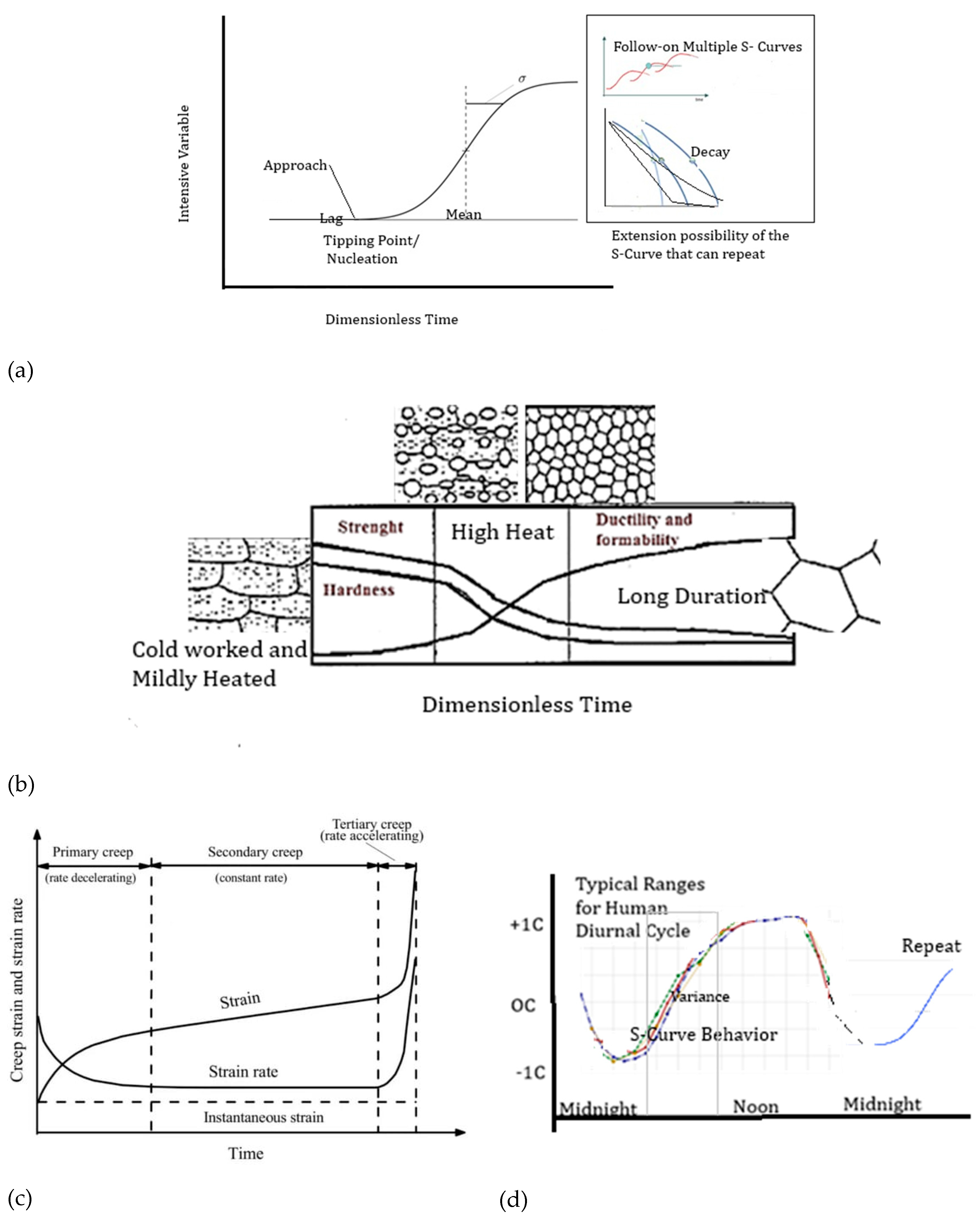
6.1. Groups of Self-Organized sub-Regions Inside a Control Volume
The sub-regions and the new order that develop within the sub-region clearly do not need to be identical. There are several cases where different types of subregions coexist in an equilibrated or slowly changing canopy (control volume), which can itself contract or expand significantly during an entropy-generating process. Figure 13 illustrates examples and schematics of such groupings [100,101,102]. Figure 13a,c are simple representations of sub-regions. However, the brain image shown in 13(b) is only a very approximate schematic representation, as this is particularly difficult to model accurately because of the complexities within and between the sub-regions [144] requiring very heavy computational resources,
Human organs within the body do not share the same temperature; there are localized differences, with some organs being slightly warmer than the core temperature and the extremities cooler due to heat loss. The body maintains an overall core temperature of about 37°C (98.6°F), but this is an average; individual organs and body parts can have minor variations. A recent study shows that the healthy human brain temperature varies significantly by region, with deeper brain areas often exceeding 40°C, and it can fluctuate throughout the day and differ between individuals due to factors such as age, sex, and menstrual cycles [129]. These temperatures affect the boundaries between elements of self-similar, organized patterns in contact with each other [52,126,127,128,129,130]. We have not investigated how variations in the subgrouping of otherwise self-similar patterns affect a system’s energy efficiency, resilience, or utility when it interacts with its surroundings.
7. Summary and Concluding Remarks
In physical systems, local fluctuations can trigger events that lead to the formation of a new order, accompanied by the emergence of new disorder at sub-boundaries. This can occur in a control volume that reaches a tipping point. The tipping point can be nucleation (e.g., a first-order transformation), spinodal decomposition (a second-order transformation), or mixed-order transformations [4], which are unstable because they can produce more entropy before reaching a more metastable or equilibrium-like condition, including oscillatory reactions that form ordered patterns, such as BZ reactions. The consequences of such processes could include the creation of new boundaries and the competitive storage of energy, or the creation of new pathways in sub-regions, as reflected in the rate of entropy generation.
Resilience is a context-dependent property. The emergence of resilience is a scale-dependent phenomenon. The S-Curve provides a contextual indication of which types of new resilience emerge, as it is based on where new energy is stored and the amount of anti-work the system experiences. Sub-boundary formation and growth are important features of self-organization that define resilience in several scenario examples presented in this article. The fact that birds are known to fly in a V pattern shows resilience against exhaustion, as discussed in Sections 3 and 5. In fact, the V pattern is one of the few patterns that show dAAD/dt as being equal to zero for the entire bird flock ([5]. There is emerging evidence for new and unusual barriers that support cognitive reserves [131,132] and related resilience due to sub-boundary formation. Plant resilience to climate change involves reorganizing boundaries and de-emphasizing growth [123,137].
Thermodynamic efficiencies, when sought, lead to emergent behavior that peaks at a critical point [44,52,61]. The stability of any morphology is related to the energy stored from anti-work; this leads to contextual resilience. The relationships between yield strength, hardness, and structure are positively correlated: finer structure has higher yield strength because the number of grain boundaries increases, but only within specific regimes. Beyond the Trivedi limit (see Section 3), a morphological transformation to a glass-like structure can occur, resulting in a considerable loss of ductility; however, the compression strength remains very high. This is because the defect structure moves from a dislocation-type non-equilibrium structure to a much more lattice non-equilibrium structure that does not permit ductility but gives a low transformer loss objective. The formation of self-organized structures, particularly in living biological systems, requires minimal energy [4,5,22,44], thereby allowing neurons to form in the human brain [56,57,58] with a relatively low energy rate demand.
All entropy-generating processes result in anti-work, enabling the generation of storable power and the formation of new sub-boundary patterns. This anti-work enables various forms of resilience from the new order that forms. For entropy-generating processes, the . Individual processes that are Sigmoidal in nature can be followed by new processes or repetitive processes, thus permitting connections between discrete events due to the property of energy storage that discrete entropy-producing pathways enable for connectivity across the time dimension.
Funding
No Funding
Institutional Review Board Statement
Not applicable.
Informed Consent Statement
Not Applicable
Data Availability Statement
None except as shown in the References.
Acknowledgments
I am grateful to MHI Inc. for providing me with the space and permitting me the time to write this article.
Conflicts of Interest
None
References
- Paltridge, G.W. The steady-state format of global climate. Quart. J. Roy. Meteor. Soc. 1978, 104, 927–945. [CrossRef]
- Louise K. Comfort, Self-Organization in Complex Systems. Journal of Public Administration Research and Theory, J-PART, 4(1994):3:393-410.
- Kondepudi, D.; Prigogine, I. Modern Thermodynamics: From Heat Engines to Dissipative Structures; John Wiley & Sons: Hoboken, NJ, USA, 2015; ISBN-10:0471973947.
- Sekhar, J.A. The description of morphologically stable regimes for steady state solidification based on the maximum entropy production rate postulate. J. Mater. Sci. 2011, 46, 6172–6190. [CrossRef]
- Sekhar, J.A. An Entropic Model for Assessing Avian Flight Formations. arXiv 2022, arXiv:2204.03102.
- Martyushev, L.M. Maximum entropy production principle: History and current status. Uspekhi Fiz. Nauk 2021, 64, 586–613. [CrossRef]
- Tzafestas, S.G. Energy, Information, Feedback, Adaptation, and Self-Organization, Intelligent Systems, Control and Automation: Science and Engineering 90; Springer: Berlin/Heidelberg, Germany, 2018.
- Pave, A.; Schmidt-Lainé, C. Integrative Biology: Modelling and Simulation of the Complexity of Natural Systems. Biol. Int. 2004, 44, 13–24.
- Fath, B. Encyclopedia of Ecology, 2nd ed.; Elsevier: Amsterdam, The Netherlands, 2019.
- Niven, RK. Simultaneous Extrema in the Entropy Production for Steady-State Fluid Flow in Parallel Pipes. arXiv 2009, arXiv:0911.5014.
- Endres, R.G. Entropy production selects non-equilibrium states in multistable systems. Sci. Rep. 2017, 7, 14437.
- Wei, Y.; Shen, P.; Wang, Z.; Liang, H.; Qian, Y. Time Evolution Features of Entropy Generation Rate in Turbulent Rayleigh-Bernard Convection with Mixed Insulating and Conducting Boundary Conditions. Entropy 2020, 22, 672. [CrossRef]
- Nicolis G, Prigogine I., Self-organization in non-equilibrium systems. New York: John Wiley & Sons; 1977.
- Vita, A. Beyond Linear Non-Equilibrium Thermodynamics. In Non-Equilibrium Thermodynamics; Lecture Notes in Physics; Springer: Cham, Switzerland, 2022; Volume 1007.
- Dyke, J.; Kleidon, A. The Maximum Entropy Production Principle: Its Theoretical Foundations and Applications to the Earth System. Entropy 2010, 12, 613-630. [CrossRef]
- Reis, A.H. Use and validity of principles of extremum of entropy production in the study of complex systems. Ann. Phys. 2014, 346, 22–27. [CrossRef]
- Sekhar, J. Thermodynamics, Irreversibility and Beauty. Available online: https://encyclopedia.pub/9548 (accessed on 27 October 2025).
- Ballufi, R.W.; Allen, M.A.; Carter, W.C. Kinetics of Materials; John Wiley & Sons: Hoboken, NJ, USA, 2005.
- Wikipedia. Differential Entropy. Available online: https://en.wikipedia.org/wiki/Differential_entropy (accessed on 27 October 2025).
- Martyushev, L.M.; Zubarev, S.N. Entropy production of stars. Entropy 2015, 17, 3645–3655.
- Martyushev, L.M.; Birzina, A. Entropy production and stability during radial displacement of fluid in Hele-Shaw cell. J. Phys. Condens. Matter 2008, 20, 465102. [CrossRef]
- Turing, A.M. The molecular basis of morphogenesis. Philos. Trans. R. Soc. 1952, 37, 237.
- Bensah, Y.D.; Sekhar, J.A. Solidification Morphology and Bifurcation Predictions with the Maximum Entropy Production Rate Model. Entropy 2020, 22, 40. [CrossRef]
- Heylighen, F. The Science of Self-Organization and Adaptivity, Center; Free University of Brussels: Brussels, Belgium, 2001; p. 9.
- H. Reuter, F. Jopp, J. M. Blanco-Moreno, C. Damgaard, Y. Matsinos, and D.L. DeAngelis, Ecological hierarchies and self-organisation - Pattern analysis, modelling and process integration across scales. [CrossRef]
- Lucia, U. Maximum entropy generation and K-exponential model. Phys. A Stat. Mech. Appl. 2010, 389, 4558–4563. [CrossRef]
- Hill, A. Entropy production as the selection rule between different growth morphologies. Nature 1990, 348, 426–428. [CrossRef]
- Ziman, J.M. The general variational principle of transport theory. Can. J. Phys. 1956, 35, 1256. [CrossRef]
- Kirkaldy, J.S. Entropy criteria applied to pattern selection in systems with free boundaries. Metall. Trans. A 1985, 16, 1781–1796. [CrossRef]
- Guggenheim, E.A. (1985). Thermodynamics. An Advanced Treatment for Chemists and Physicists, seventh edition, North Holland, Amsterdam, ISBN 0-444-86951-4.
- Ziegler, H.; Wehrli, C. On a principle of maximal rate of entropy production. J. Non-Equilib. Therm. 1978, 12, 229. [CrossRef]
- Pave, A.; Schmidt-Lainé, C. Integrative Biology: Modelling and Simulation of the Complexity of Natural Systems. Biol. Int. 2004, 44, 13–24.
- Pal, R. (2019). Teaching Fluid Mechanics and Thermodynamics Simultaneously through Pipeline Flow Experiments. Fluids, 4(2), 103. [CrossRef]
- Wikipedia. Differential Entropy. Available online: https://en.wikipedia.org/wiki/Differential_entropy (accessed on 27 October 2025).
- Martyushev, L.M.; Zubarev, S.N. Entropy production of stars. Entropy 2015, 17, 3645–3655. [CrossRef]
- Heylighen, F. The Science of Self-Organization and Adaptivity, Center; Free University of Brussels: Brussels, Belgium, 2001; p. 9.
- Sánchez-Gutiérrez D. Tozluoglu M., Barry J.D., Pascual A.; Mao Y., Escuder L.M., Fundamental physical cellular constraints drive self-organization of tissues. EMBO J. 2016, 35, 77–88.
- Hill, A. Entropy production as the selection rule between different growth morphologies. Nature 1990, 348, 426–428.
- Martyushev, L.M.; Seleznev, V.D.; Kuznetsova, I.E. Application of the Principle of Maximum Entropy production to the analysis of the morphological stability of a growing crystal. Zh. Éksp. Teor. Fiz. 2000, 118, 149.
- Onsager, Lars (1931-02-15). "Reciprocal Relations in Irreversible Processes. I." Physical Review. 37 (4). American Physical Society (APS): 405–426. Bibcode:1931PhRv...37..405O ISSN 0031-899X. [CrossRef]
- Miller, Donald G. (1960). "Thermodynamics of Irreversible Processes. The Experimental Verification of the Onsager Reciprocal Relations". Chemical Reviews. 60 (1). American Chemical Society (ACS): 15–37. ISSN 0009-2665. [CrossRef]
- Crosato, E., Spinney R.E., Nigmatullin, R., Lizier, J.T., Prokopenko M. Thermodynamics and computation during collective motion near criticality. Phys. Rev. E 2018, 97, 012120. [CrossRef]
- Joardar J., Lele S., Rama Roa P. Notes on Thermodynamics of Materials, T.R. Anantharaman Education and Research Foundation (www.tra-erf.org); First Edition (1 January 2016).
- J A. Sekhar An Entropy Generation Rate Model for Tropospheric Behavior That Includes Cloud Evolution, Entropy 2023, 25(12),1625. [CrossRef]
- Gibbins, G.; Haigh, J.D. Entropy Production Rates of the Climate. J. Atmos. Sci. 2022, 77, 3551–3566. [CrossRef]
- Wu, W.; Liu, Y. Radiation entropy flux and entropy production of the Earth system. Rev. Geophys. 2010, 48, 2008RG000275. [CrossRef]
- Kurz W, Fisher TJ (2003) Solidification. Trans Tech Publications, Switzerland.
- Chalmers B (1964) Principles of solidification. John Wiley & Sons, New York.
- Flemings MC (1974) Solidification processing. McGraw-Hill, New York.
- J.A. Sekhar, H.P. Li, G.K. Dey, Decay-dissipative Belousov–Zhabotinsky nanobands and nanoparticles in NiAl Acta Materialia, Volume 58, Issue 3, February 2010, Pages 1056-1073.
- Kohler JM, Muller SC. J Phys Chem 1995;99:980–3.
- Sekhar, J.A. Self-Organization, Entropy Generation Rate, and Boundary Defects: A Control Volume Approach. Entropy 2021, 23, 1092. [CrossRef]
- Jonathan H. McCoy*, Will Brunner, Werner Pesch, Phys. Rev. Lett. 101, 254102. [CrossRef]
- Fabietti, L.M., Sekhar, J.A. Planar to equiaxed transition in the presence of an external wetting surface. Metall Trans A 23, 3361–3368 (1992). [CrossRef]
- Bruce E. Shaw. (accessed on 27 October 2025). [CrossRef]
- P. R. Hiesinger, The Self-Assembling Brain: How Neural Networks Grow Smarter, ISBN 9780691181226, Princeton University Press, 2021.
- I.M. De La Fuente, L. Martínez, A. L. Pérez-Samartín, L. Ormaetxea, C. Amezaga, A. Vera-López, Global Self-Organization of the Cellular Metabolic Structure. PLoS ONE 2008, 3(8): e3100. [CrossRef]
- L. A. Blumenfeld and H. Haken (Eds), Problems of Biological Physics, Springer Berlin Heidelberg, ISBN 9783642678530, 2016.
- 59. K. Somboonsuk, J.T. Mason, and R. Trivedi: Metall. Trans. A, vol. 15A, pp. 967–75, 1984. See also R. Trivedi and K. Somboonsuk, Constrained Dendritic Growth and Spacing, Materials Science and Engineering, 65, pp. 65-74,1984. [CrossRef]
- Proceedings of the 2nd International Conference on Rapid Solidification Processing, eds R. Mehrabian, B. H. Kear and M. Cohen, Claitor’s Publishing Division, Baton Rouge, LA., Reston, VA, pp. 153–164, 1980.
- R. Nigmatullin and M. Prokopenko, Thermodynamic Efficiency of Interactions in Self-Organizing Systems. Entropy, 23, 757, 2021. [CrossRef]
- Bensah, Y.D.; Sekhar, J.A. Interfacial instability of a planar interface and diffuseness at the solid-liquid interface for pure and binary materials. arXiv 2016, arXiv:1605.05005.
- Bensah, Y.D.; Sekhar, J.A. Morphological assessment with the maximum entropy production rate (MEPR) postulate. Curr. Opin. Chem. Eng. 2014, 3, 91–98. [CrossRef]
- Li H.P., Dissipative Belousov–Zhabotinsky reaction in unstable micropyretic synthesis, Current Opinion in Chemical Engineering, Volume 3, February 2014, Pages 1-6. [CrossRef]
- https://en.wikipedia.org/wiki/Fractal (accessed on 27 October 2025).
- Mandelbrot, Benoît B. (1983). The fractal geometry of nature. Macmillan. ISBN 978-0-7167-1186-5.
- Gouyet, Jean-François (1996). Physics and fractal structures. Paris/New York: Masson Springer. ISBN 978-0-387-94153-0.
- Chen Y., Equivalent relation between normalized spatial entropy and fractal dimension, Physica A: Statistical Mechanics and its Applications, Volume 553, 2020, 124627, ISSN 0378-4371. [CrossRef]
- Sekhar J. A. (2018). Tunable Coefficient of Friction with Surface Texturing in Materials Engineering and Biological Systems.Current Opinion in Chemical Engineering, 19,94.
- Sekhar, J.A., Mantri, A.S., Yamjala, S. et al. Ancient Metal Mirror Alloy Revisited: Quasicrystalline Nanoparticles Observed. JOM 67, 2976–2983 (2015). [CrossRef]
- Cengel Y, and Boles, Thermodynamics, McGraw-Hill Seventh Edition, ISBN 9780073529325, 2011.
- https://en.wikipedia.org/wiki/Patterns_in_nature (accessed on 27 October 2025).
- https://en.wikipedia.org/wiki/Minimal_surface (accessed on 27 October 2025).
- J. A. Sekhar A. S. Mantri, Sabyasachi Saha, R. Balamuralikrishnan, P. Rama Rao, Trans Indian Inst Met. [CrossRef]
- Sekhar, J.A.; Mohan, M.; Divakar, C.; Singh, A.K., Rapid solidification by high-pressure application. Scr. Metall. 1984, 18, 1327–1330.
- Levi, C.G.; Mehrabian, R. Heat flow during rapid solidification of undercooled metal droplets. Metall. Trans. A 1982, 13A, 221–234. [CrossRef]
- https://www.youtube.com/watch?v=axEExcI5k4E (accessed on 27 October 2025).
- Garfinkel A, Tintut Y, Petrasek D, Boström K, Demer LL. Pattern formation by vascular mesenchymal cells. Proc Natl Acad Sci U S A. 2004 Jun 22;101(25):9247-50. Epub 2004 Jun 14. PMID: 15197273; PMCID: PMC438961. [CrossRef]
- Sekhar J. A., and Sivakumar R., 1985, On the improvement of fatigue resistance of Ti-4A-6V castings, Journal of Materials Research, volume 4, 1985, pp. 144- 146.
- Bhaduri, S., Sekhar, J. Mechanical properties of large quasicrystals in the Al–Cu–Li system. Nature 327, 609–610 (1987). [CrossRef]
- Bejan A. Advanced engineering thermodynamics. John Wiley & Sons; 2016 Sep 19.
- Carteret, H.; Rose, K.; Kauffman, S. Maximum Power Efficiency and Criticality in Random Boolean Networks. Phys. Rev. Lett. 2008, 101, 218702.
- Barato, A.; Hartich, D.; Seifert, U. Efficiency of cellular information processing. New J. Phys. 2014, 16, 103024.
- Kempes, C.; Wolpert, D.; Cohen, Z.; Pérez-Mercader, J. The thermodynamic efficiency of computations made in cells across the range of life. Philos. Trans. R. Soc. Math. Phys. Eng. Sci. 2017, 375. [CrossRef]
- M. Luebbe et al., Microstructural Evolution in a Precipitate-Hardened (Fe0.3Ni0.3Mn0.3Cr0.1)94Ti2Al4 Multi-Principal Element Alloy during High-Pressure Torsion, Journal of Materials Science, vol. 59, no. 28, pp. 13200 - 13217, Springer, Jul 2024.
- Dey GK, Sekhar JA (1997), Micropyretic synthesis of tough NiAl alloys. Metall. Mater. Trans. B 28(5):905–918.
- Begehr, H., & Wang, D. (2025). Beauty in/of mathematics: tessellations and their formulas. Applicable Analysis, 104(14), 2826–2872. [CrossRef]
- Ho, C.T., Cheng, C.J. & Sekhar, I.A. Solidification microporosity in directionally solidified multicomponent nickel aluminide. Metall Trans A 22, 225–234 (1991). [CrossRef]
- Trivedi R., Directional solidification of alloys. Principles of Solidification and Materials Processing. New Delhi: Oxford and IBH Publishers; 1988. p. 3–65.
- https://en.wikipedia.org/wiki/Kolmogorov_microscales.
- Roberto Benzi, Federico Toschi, 2023, Lectures on Turbulence, Physics Reports, 1021, P1-106. [CrossRef]
- Bird, R.B.; Stewart, W.E.; Lightfoot, E.N. Transport Phenomena, 2nd ed.; Wiley: New York, NY, USA, 2007.
- Sekhar JA, Journal of Crystal Growth, Volume 109, Issues 1–4, 2 February 1991, Pages 113-119.
- Trivedi RK., Sekhar JA., Seetharaman V. Metallurgical Transactions A, Volume 20A, April 1989, page 769.
- Douglas Gouvêa, 2024, Thermodynamics of solid-state sintering: Contributions of grain boundary energy, Journal of the European Ceramic Society, Volume 44, Issue 14.
- Hoge Ce, Pask JA, 1977, Ceramurgia International, Volume 3, Issue 3, July–September 1977, Pages 95-99.
- Pozzoli VA, Ruiz MS, Kingston D.,Razzitte AC., Procedia Materials Science 8 (2015), 1073 – 1078.
- Non-negligible entropy effect on sintering of supported nanoparticles, https://arxiv.org/pdf/2204.00812 (accessed on 27 October 2025).
- Vissa, A. A., & Sekhar, J. A. (2025). Technical Trends, Radical Innovation, and the Economics of Sustainable, Industrial-Scale Electric Heating for Energy Efficiency and Water Savings. Sustainability, 17(13), 5916. [CrossRef]
- https://en.wikipedia.org/wiki/Entropy_production(accessed on 17 November 2025).
- https://en.wikipedia.org/wiki/Human_brain (accessed on 27 October 2025).
- https://montanaballoon.com/fun-and-colorful-shaped-hot-air-balloons.php (accessed on 27 October 2025).
- Schobeiri, M.T. (2022). Turbulent Flow, Modeling. In: Advanced Fluid Mechanics and Heat Transfer for Engineers and Scientists. Springer, Cham. [CrossRef]
- Sekhar JA., 2020 Rapid solidification and surface topography for additive manufacturing with beam surface heating, Current Opinion in Chemical Engineering, Volume 28, June 2020, Pages 10-20.
- T. C. Wiiliams, T. J. Klonowski and P. Berkely, The Auk 93, pg. 554-559, 1976.
- https://www.allaboutbirds.org/guide/Canada_Goose/id last accessed December 28, 2022.
- P. B. Lissaman and C. A. Shollenberger, Formation Flight of Birds, Science vol. 168, 1970 pg. 1003-1005.
- Noether, E. Invariante Variations probleme. Nachr. d. König. Gesellsch. d. Wiss. zu Göttingen, Math.-Phys. Klasse 235 (1918). English translation by Tavel, M. A. Invariant variation problems. Transp. Theo. Stat. Phys. 1, 186 (1971).
- Hermann, S., Schmidt, M. Noether’s theorem in statistical mechanics. Commun Phys 4, 176 (2021). [CrossRef]
- L. Luke et. Al., Architectural immunity: Ants alter their nest networks to prevent epidemics, Science, 390,266-271(2025). [CrossRef]
- Brandon Shuck, Brian Boston, Suzanne M. Carbotte, Shuoshuo Han, Anne Bécel, Nathaniel C. Miller, J. Pablo Canales, Jesse Hutchinson, Reid Merrill, Jeffrey Beeson, Pinar Gurun, Geena Littel, Mladen R. Nedimović, Genevieve Savard, Harold Tobin. Slab tearing and segmented subduction termination driven by transform tectonics. Science Advances, 2025; 11 (39). [CrossRef]
- ScienceDaily, 25 October 2025. www.sciencedaily.com/releases/2025/10/251025084616.htm. Last accessed October 24, 2025.
- V. K. Vasudevan and J. A. Sekhar, "Transformation Behavior in Nanoscale Binary Aluminum Alloys," in: Advances in the Metallurgy of Aluminum Alloys, TMS, Warrendale, PA, pp. 398- 405 (2001). Reproduced at the repostiary https://mhi-inc.com/wp-content/uploads/2018/10/Nano-aluminum-alloys-sponsored-by-MHI.pdf.
- N. Dey, J.A. Sekhar Interface configurations during the directional growth of Salol—I. Morphology, Acta Metallurgica et Materialia, Volume 41, Issue 2,1993, Pages 409-424. [CrossRef]
- R. Cheese and B. Cantor, Mater. Sci. Eng, 45, 83 (1980).
- Ye, P.; Yang, C.; Li, Z.; Bao, S.; Sun, Y.; Ding, W.; Chen, Y. Texture and High Yield Strength of Rapidly Solidified AZ31 Magnesium Alloy Extruded at 250 °C. Materials 2023, 16, 2946. [CrossRef]
- Bejan, A., Lorente, S., Yilbas, B. et al. Why solidification has an S-shaped history. Sci Rep 3, 1711 (2013). [CrossRef]
- Szyszka, T.N., Wijaya, D.S., Siddiquee, R. et al. Reprogramming encapsulins into modular carbon-fixing nanocompartments. Nat Commun 16, 9493 (2025). [CrossRef]
- Zuo, H., Tian, F., Zhang, C. et al. A universal entropic pulling force caused by binding. Nat Commun 16, 9604 (2025). [CrossRef]
- Romanenko, A.; Vanchurin, V. Quasi-Equilibrium States and Phase Transitions in Biological Evolution. Entropy 2024, 26, 201. [CrossRef]
- Connelly, Michael C. & Sekhar, J.A., 2012. "U. S. energy production activity and innovation," Technological Forecasting and Social Change, Elsevier, vol. 79(1), pages 30-46.
- Joseph Swift, Leonie H. Luginbuehl, Lei Hua, Tina B. Schreier, Ruth M. Donald, Susan Stanley, Na Wang, Travis A. Lee, Joseph R. Nery, Joseph R. Ecker, Julian M. Hibberd. Exaptation of ancestral cell-identity networks enables C4 photosynthesis. Nature, 2024. [CrossRef]
- www.sciencedaily.com/releases/2025/11/251109032410.htm (accessed on 27 October 2025).
- Bhaduri, S., Sekhar, J. Mechanical properties of large quasicrystals in the Al–Cu–Li system. Nature 327, 609–610 (1987). [CrossRef]
- https://www.researchgate.net/profile/Birgitte-Andersen-2/publication/24058325_The_hunt_for_S-shaped_growth_paths_in_technological_innovation_A_patent_study/links/00b49526a2fddc408c000000/The-hunt-for-S-shaped-growth-paths-in-technological-innovation-A-patent-study.pdf (accessed on 27 October 2025).
- Vellei, M., Pigliautile, I. & Pisello, A.L. Effect of time-of-day on human dynamic thermal perception. Sci Rep 13, 2367 (2023). [CrossRef]
- Huus, L. M., & Ley, R. E. (2021). Blowing Hot and Cold: Body Temperature and the Microbiome. mSystems, 6(5), e00707-21.
- Ali Asgary. https://medium.com/@ali.asgary/can-we-sharpen-the-recovery-curve-48e45111922a.
- https://neurosciencenews.com/brain-termperature-20816.
- Gales, J., Bisby, L.A., and Strafford, T (2012) New Parameters to Describe High Temperature Deformation of Prestressing Steel determined using Digital Image Correlation. StructuralEngineering International. 22 (4). 476-486. [CrossRef]
- Reed-Hill RE, Abbaschian R (1994) Physical metallurgy principles, 3rd edn. PWS Publishing Company, Boston.
- Jones, David R. H., and Michael F. Ashby. 2019. Engineering Materials 1: An Introduction to Properties, Applications and Design. 5th ed. Oxford: Butterworth-Heinemann/Elsevier.
- Bialystok, Ellen et al., 2012, Trends in Cognitive Sciences, Volume 16, Issue 4, 240 - 250.
- Silva, A.B., Liu, J.R., Metzger, S.L. et al. A bilingual speech neuroprosthesis driven by cortical articulatory representations shared between languages. Nat. Biomed. Eng 8, 977–991 (2024). [CrossRef]
- Dierk Raabe, 2014 Chapter 23 - Recovery and Recrystallization: Phenomena, Physics, Models, Simulation, Eds., David E. Laughlin, Kazuhiro Hono, Physical Metallurgy (Fifth Edition), Elsevier, Pages 2291-2397.
- Rest, J, 2012, Comprehensive Nuclear Materials Volume 3, Pages 579-627.
- Kumar A, Muthuramalingam P, Kumar R, Tiwari S, Verma L, Park S, Shin H. Adapting Crops to Rising Temperatures: Understanding Heat Stress and Plant Resilience Mechanisms. Int J Mol Sci. 2025 Oct 27;26(21):10426. PMID: 41226465; PMCID: PMC12608908. [CrossRef]
- Rao, PV, and Sekhar JA, April 1985, Materials Letters 3(5-6):216-218. [CrossRef]
- P. D. S. de Lima et al, Self-assembled clusters of mutually repelling particles in confinement, Physical Review E (2025). On arXiv: DOI: 10.48550/arxiv.2506.19772. [CrossRef]
- Wei Deng, Zihao Wang, Jingmin Wang, Tao Hu, Xiao Wang, Xuemei Li, Jun Yin, Wanlin Guo. Floating droplet electricity generator on water. National Science Review, 2025; 12 (11). [CrossRef]
- Wenchao Hu, Xueliang Zhang, Siyuan Yi, Haijun Wang, Bangchun Wen, Self-synchronization and self-balancing characteristics of a space two rotor system, International Journal of Mechanical Sciences, Volume 303,2025,110673.
- https://youtu.be/_uTPiBlcZpg accessed November 17, 2025.
- Reddy G.S., and Sekhar J. A., Moderate pressure solidification: Undercooling at moderate cooling rates, 1989, Acta Metallurgica 37(5):1509-1519. [CrossRef]
- Allen Institute. "Supercomputer creates the most realistic virtual brain ever." ScienceDaily. www.sciencedaily.com/releases/2025/11/251118212037.htm (accessed November 18, 2025).
Figure 1.
Entropy generation and self-organization can happen at various scales. (a, b, c) Self-organized and self-similar structures in cast (frozen) solids in a Cu-Sn alloy [70,74] at various scales of magnification. Figures in (d, e) are pictures of entropy-generating non-equilibrium clouds with various scales of repetitive self-similar patterns [44]. The picture in 2(d) shows a streetlamp for scale assessment within a viewing angle of ~20 degrees. See reference [4] for the contextual assessment of self-similarity in the development of self-similar groups of rainclouds and their similarity to the grain and other microstructural features in a metallic crystalline object.
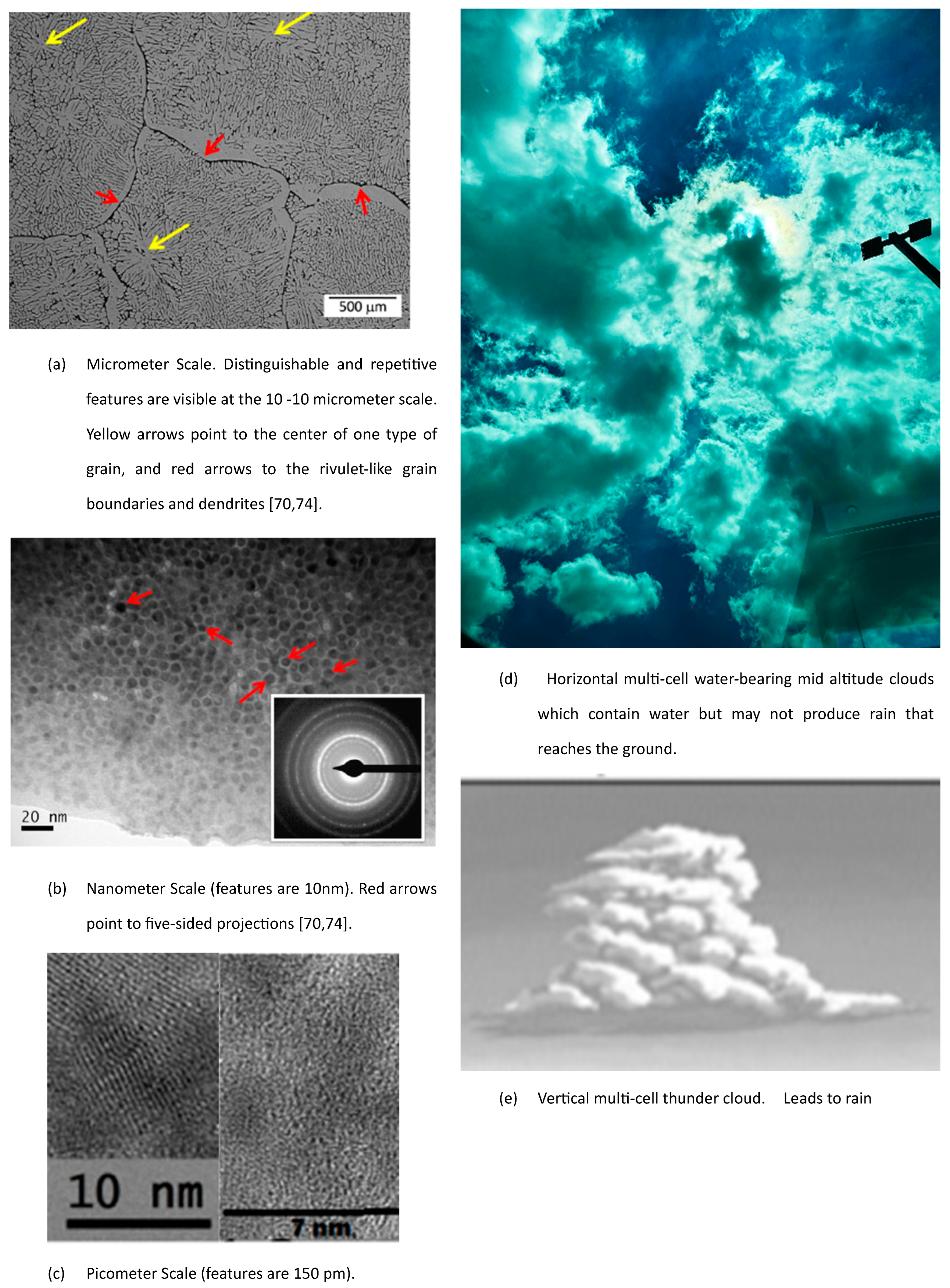
Figure 2.
Millimeter, Micrometer, and Nanometer scale for Banded Self-Organizing (oscillating structures) and striations in Condensed Matter. Adapted from Reference [50,51,64,79,80].
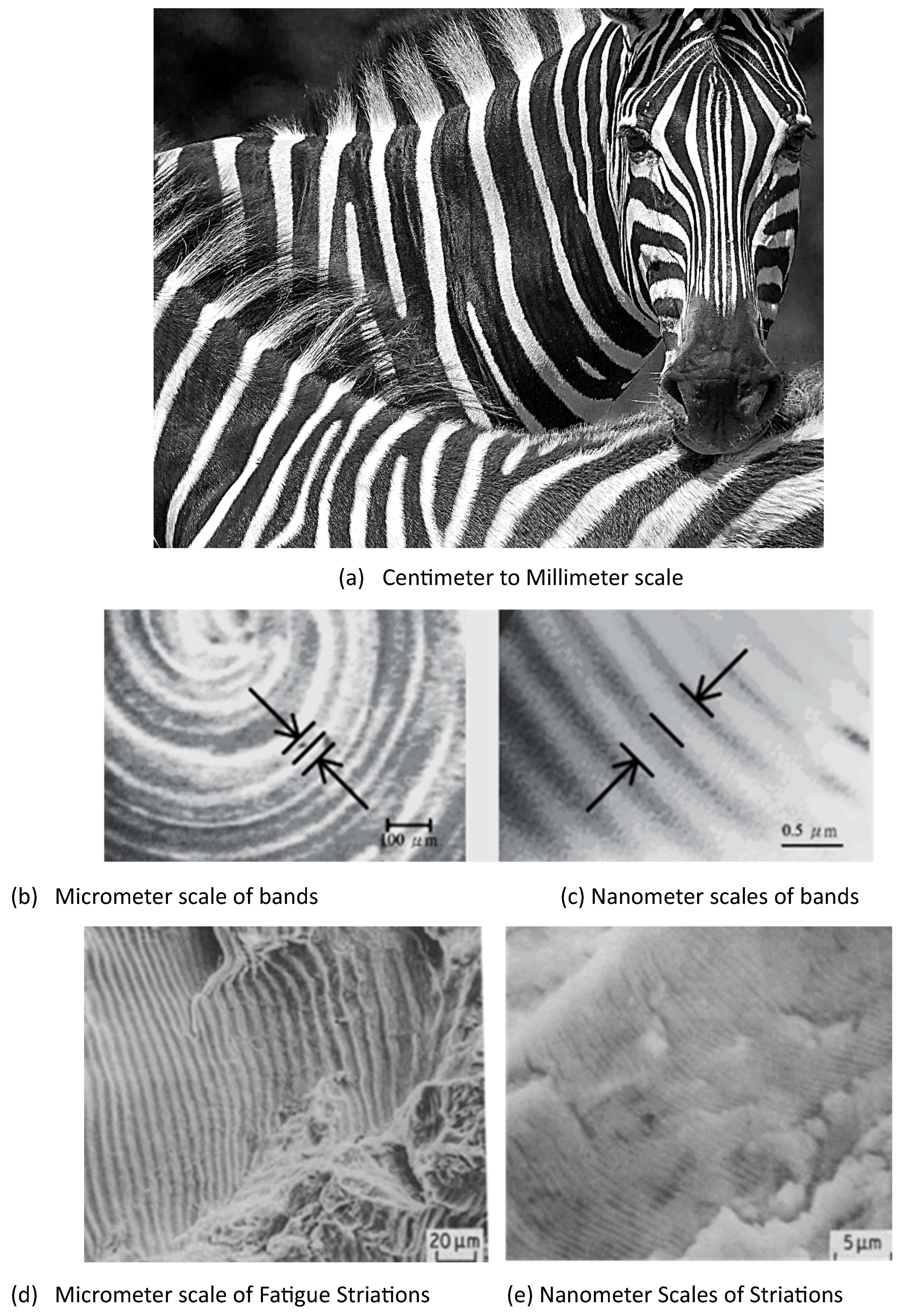
Figure 3.
Possible pathways in self-organizing systems, typified, for example, by liquid droplet undercooling, which is discussed in detail in Section 4 of this article. Process pathways and potential metastable equilibria are illustrated in Figure 3 (a) for Cooling [76] and Rapid Pressurization (b) references [75,138,143]. Paths A and B [143] show one or many metastable states, respectively. Path C shows no identifiable metastable states, and there is no intermediate heating from recalescence. After the recalescence, following a metastable event, the decay towards equilibrium is typically exponential unless another metastable equilibrium is encountered. Resting in metastable states is illustrated by a ball at rest.
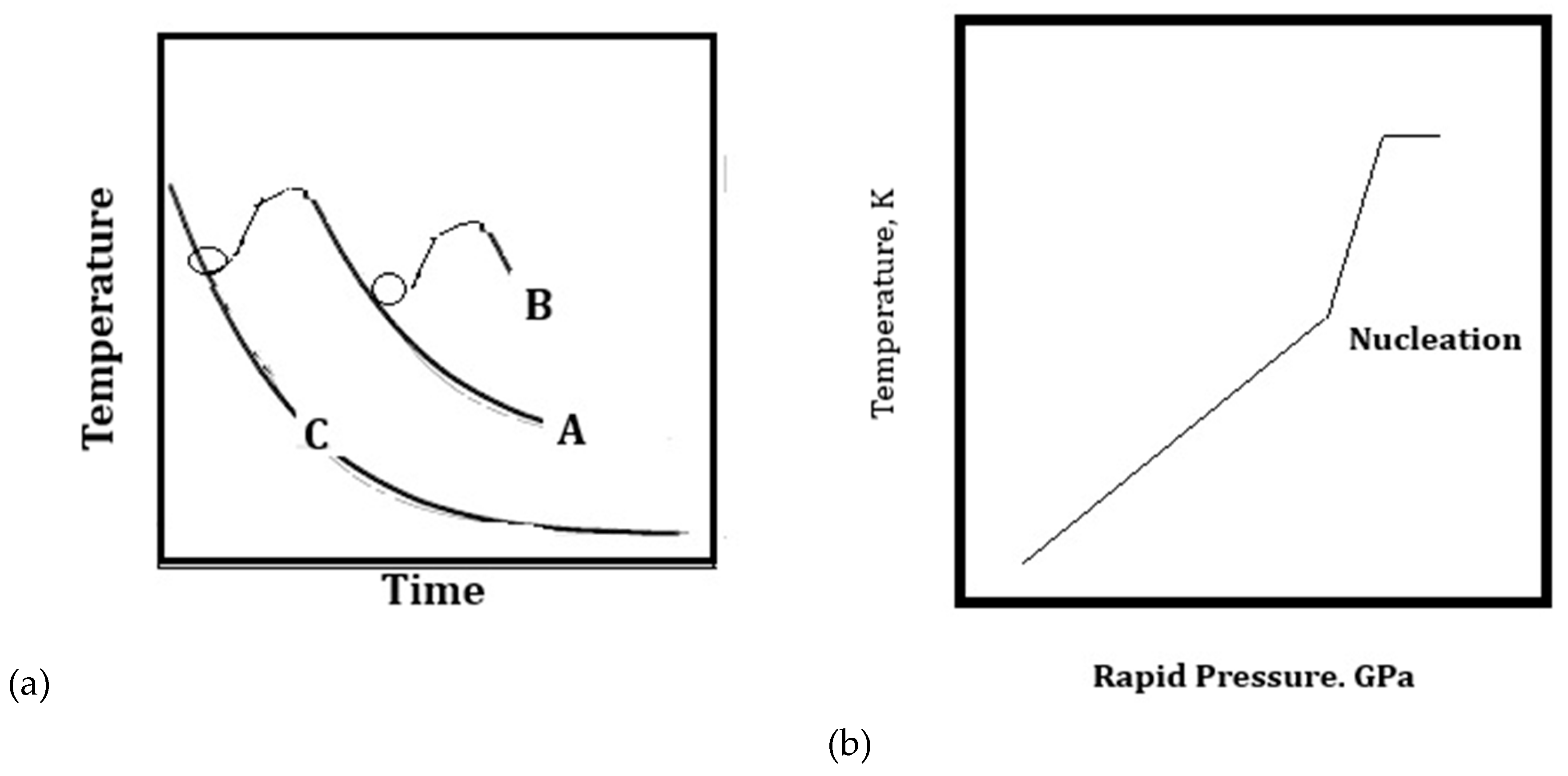
Figure 4.
(a). A diagrammatic description of the temperature and entropy density, the heat flow rate between two reservoirs, entropy generation rate, and power rate in a bar with length L, cross-sectional area A, and thermal conductivity κ. The heat flow rate is Q̇ (J/s) from T1 to T0 (with T1 > T0), at steady state, where both temperatures are reservoirs. This is a steady-state, irreversible pathway defined by local equilibrium conditions. The bar is adiabatic except at its two ends. Figure 4 (b) shows a reversible heat engine between T1 and T0, which yields a Pmax that depends on the heat transfer coefficient (J/m²Ks) and the area of contact A with the thermal reservoirs.
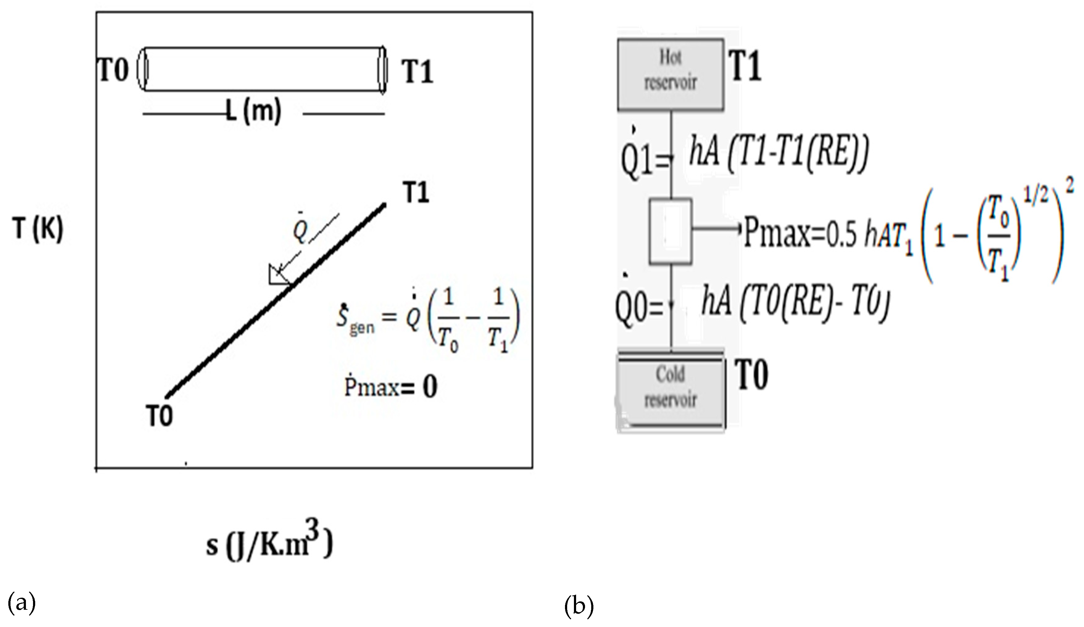
Figure 5.
The loss of efficiency as a function of the ratio of the lower reservoir temperature to the higher reservoir temperature.
Figure 5.
The loss of efficiency as a function of the ratio of the lower reservoir temperature to the higher reservoir temperature.
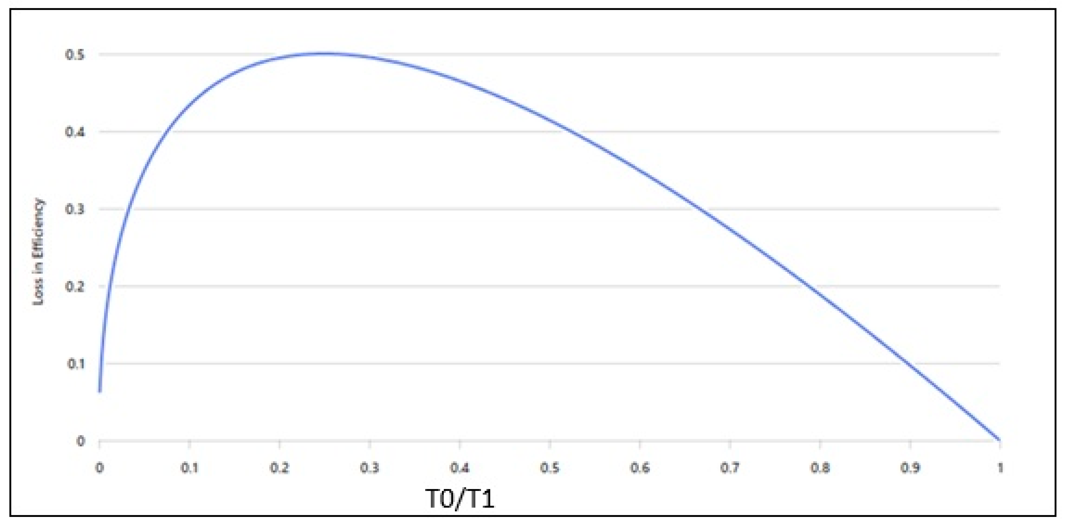
Figure 6.
For the patterns formed by birds in (c) when they self-organize into a V-shape, which conserves energy, the energy rate expenditure and rate of entropy generation rate divided by the energy rate per unit bird is shown in (c). A plot β (K-1) (Entropy generation rate divided by the rate of energy expenditure per bird), as a function of the distance from the bird center, is shown in (d) for a 3 Bird flock (from reference [5]). The inset is a picture of V formations from http://www.strategistblog.com/2020/10/flying-in-remote-formation.html.
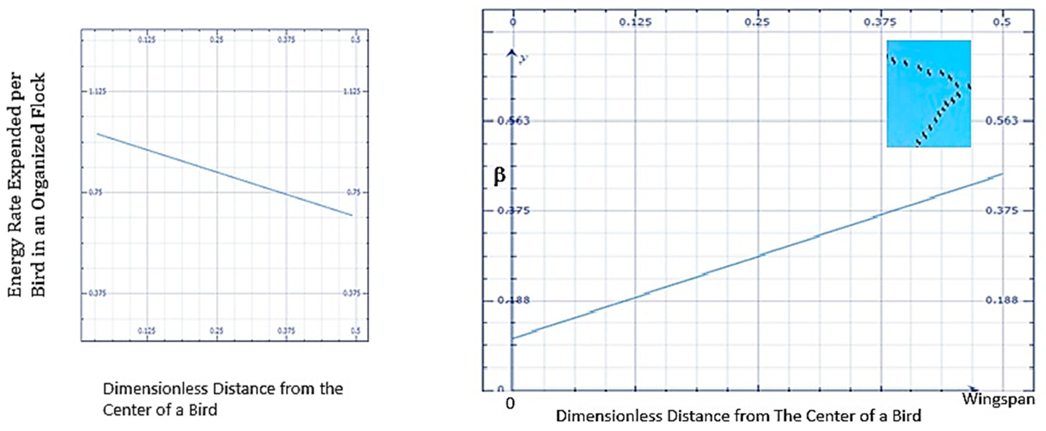
Figure 8.
Plot of l1 (primary arm spacing) vs l2 (secondary arm spacing) from the MEPR condition. Dendrite figure with l1 (primary arm spacing) vs l2 from reference [89] used with permission.
Figure 8.
Plot of l1 (primary arm spacing) vs l2 (secondary arm spacing) from the MEPR condition. Dendrite figure with l1 (primary arm spacing) vs l2 from reference [89] used with permission.
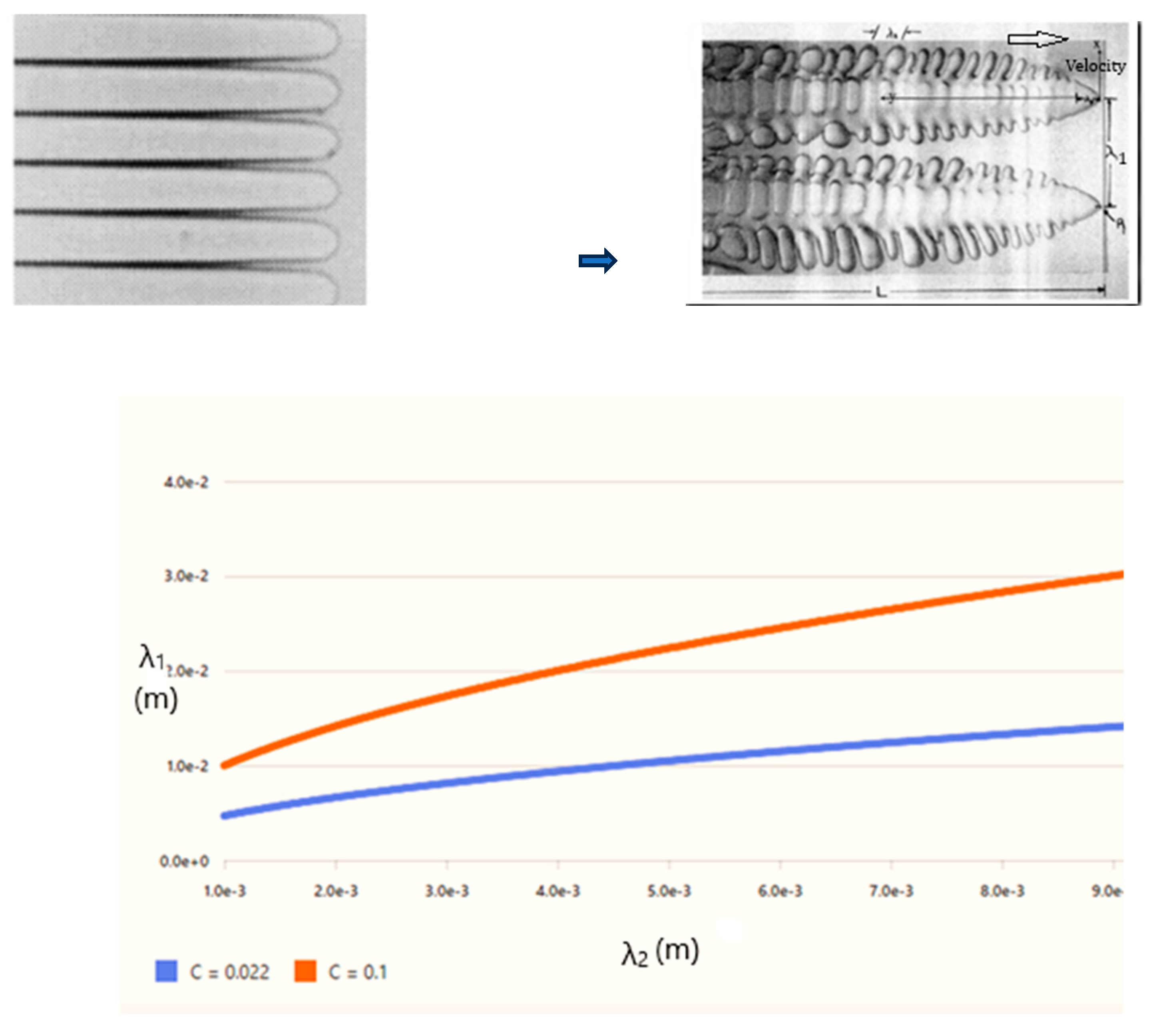
Figure 9.
The shape of the cooling curve is obtained from only considering that the second differential of the entropy generation, i.e., the first differential of the entropy generation rate, is equal to zero.
Figure 9.
The shape of the cooling curve is obtained from only considering that the second differential of the entropy generation, i.e., the first differential of the entropy generation rate, is equal to zero.
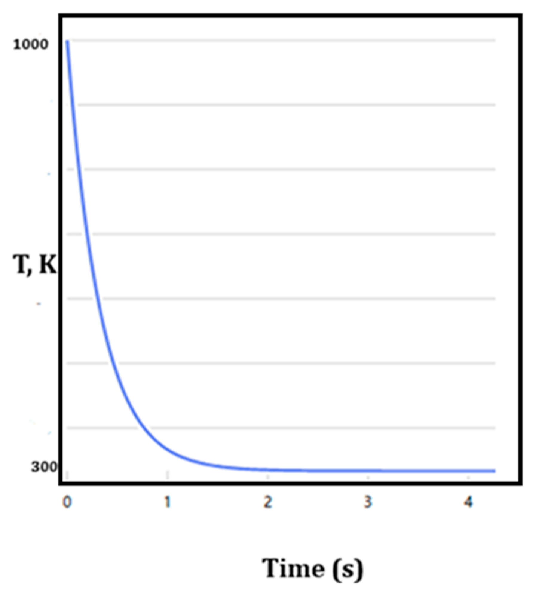
Figure 10.
Recalescence of an aluminum metal droplet. The only external kinetic factor assumed was that the interface growth rate was proportional to the interface undercooling. Aluminum melts at 933K. The nucleation temperature was arbitrarily assumed to be 700K. We approximated the velocity of the solid liquid in the interface, v, as equal to a constant Kc (m/Ks) multiplied by the undercooling, making it proportional to - (T-Tm), where Tm is the melting point of aluminum. Kc was assumed to be 0.1(m/Ks). Figure 9(c) is a generic second differential. i.e., the PDF/CDF of the normal distribution (representative of the entropy generation rate).
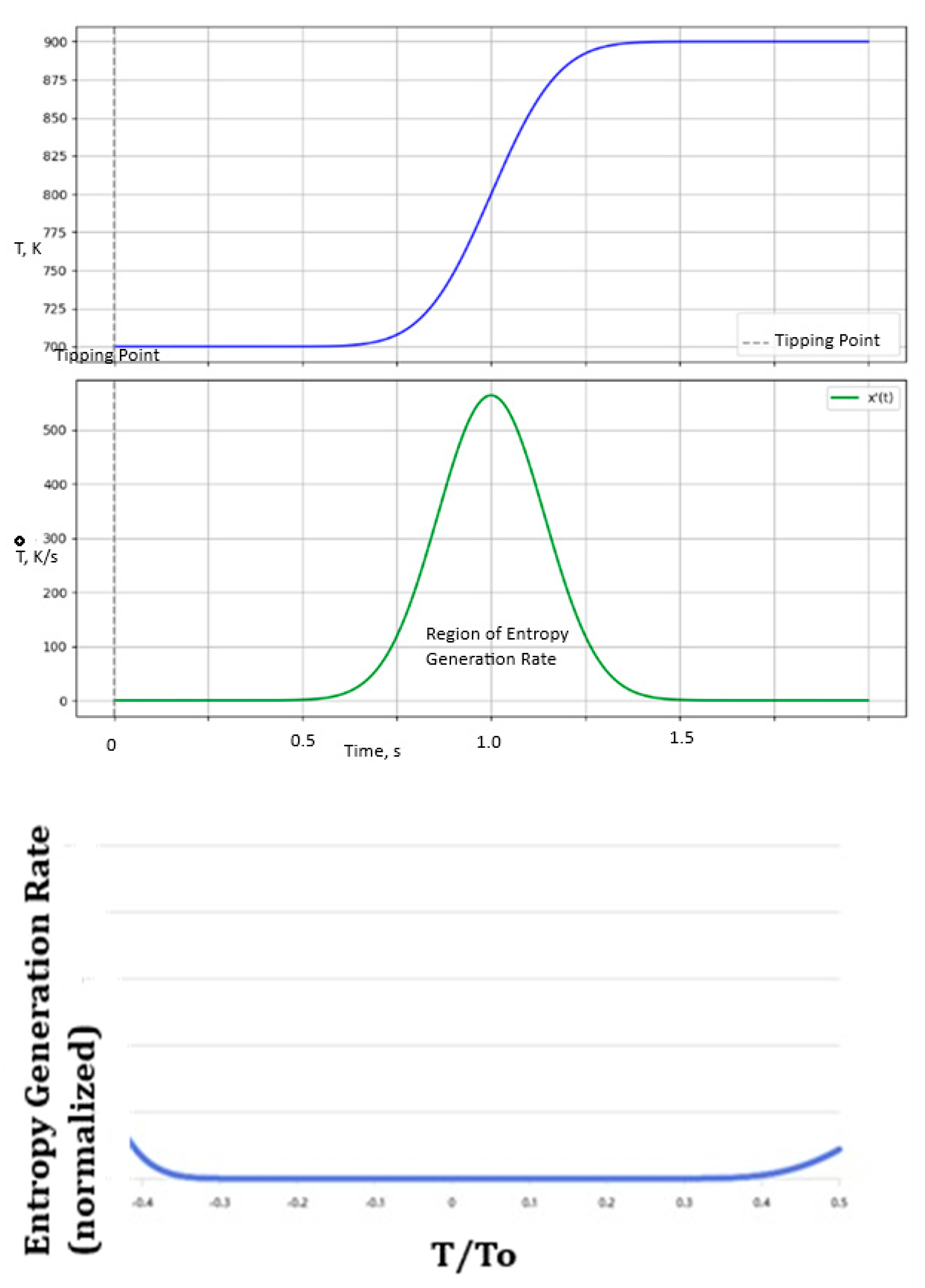
Figure 11.
The rate of sub-boundary creation is shown along with the S-curve, both plotted on a logarithmic scale.
Figure 11.
The rate of sub-boundary creation is shown along with the S-curve, both plotted on a logarithmic scale.
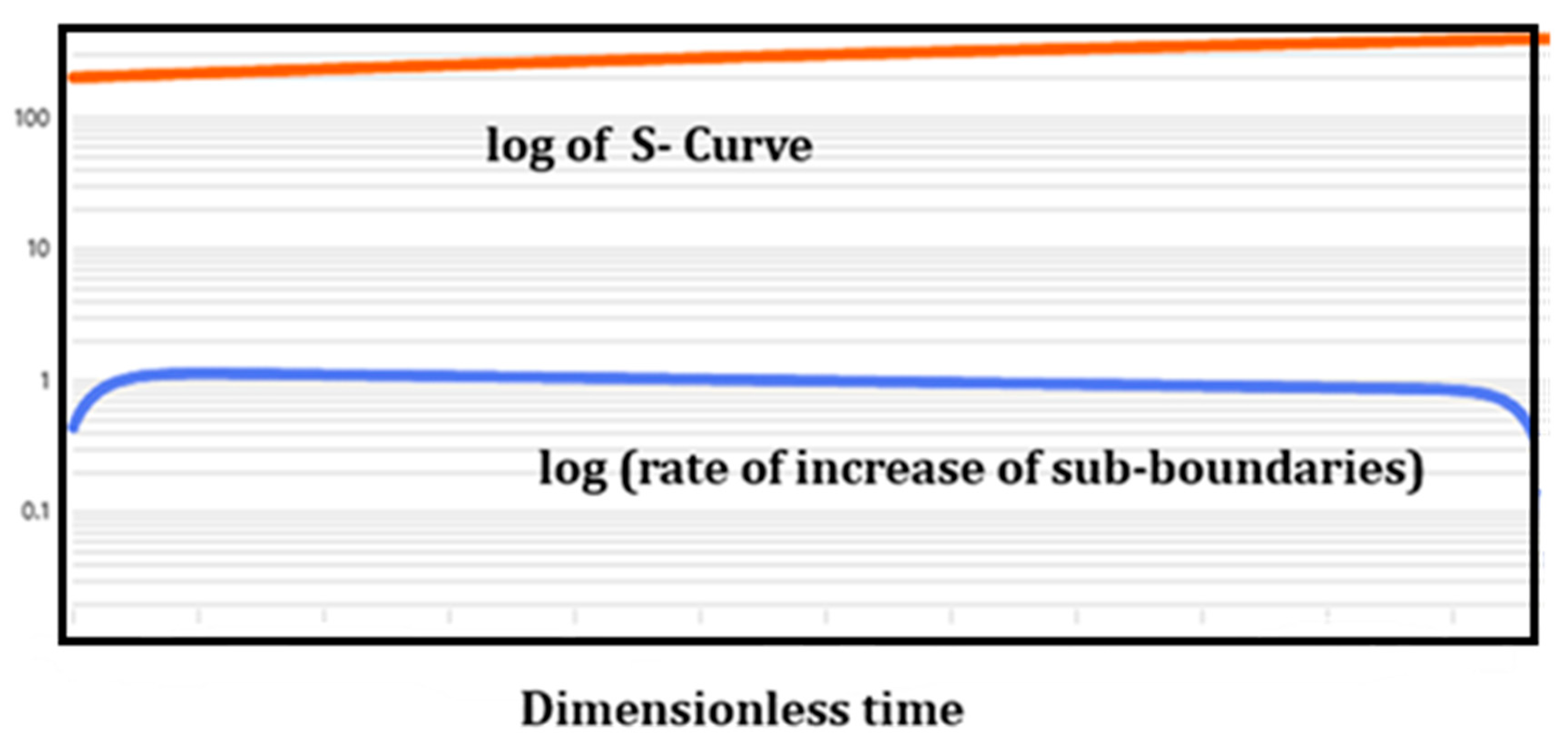
Figure 12.
(a)An illustration of boundary formation after nucleation and a rapid growth process that involves a change in morphology from boundary-free to constant boundary creation. A TEM bright field image of the Al-Zn particles aged at 130 °C for 1 hour. Note the two types of transformations noted in the particle, namely precipitates labeled A and the serrated structure labeled B (bottom picture): A TEM bright field image of the Al-Zn particles aged at 130 °C for 1 hour. The dark particle in the center of the photomicrograph is pure Zn. Note the facets in this particle (from reference [113]). Facets appear as straight-line boundaries at high magnification, whereas curved boundaries are observed at lower magnification. Note that tip undercooling in alloys can also alter facet angles, as discussed in reference [114]. A change in facet angle can also change the boundary spacing. (a) Showing bimodal sub-boundary envelopes following a path of several metastable recalescence events [143] as shown in Path B of Figure 3.
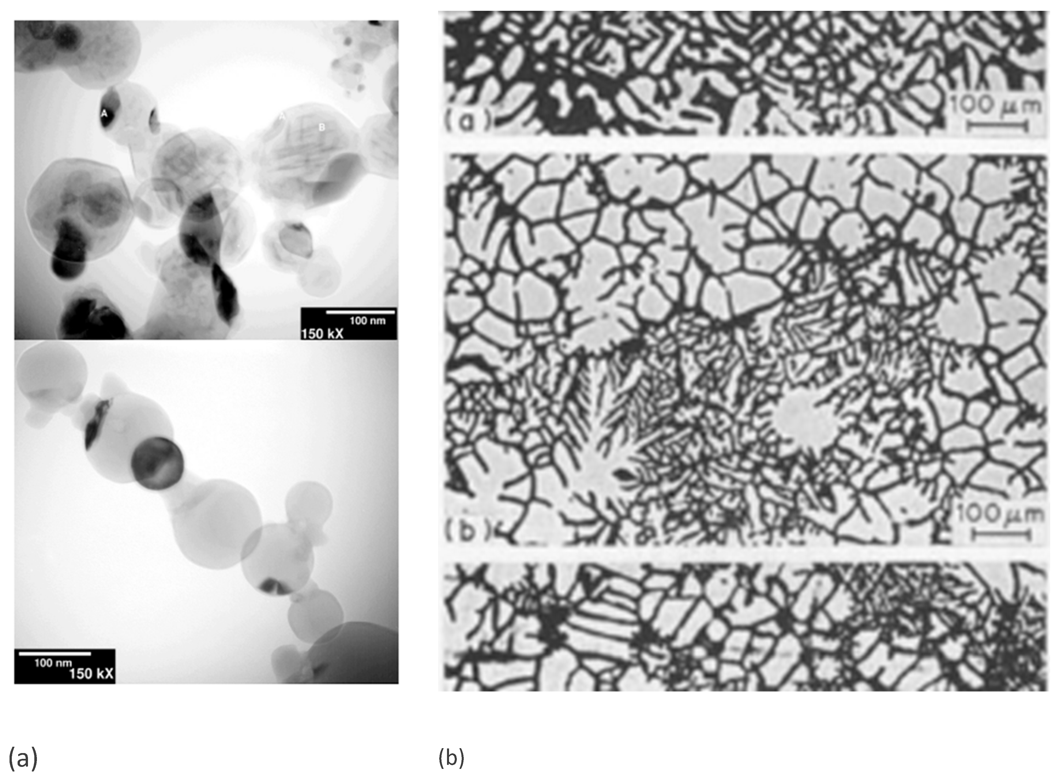
Figure 13.
(a) General representation of an inhomogeneous system that comprises interacting subsystems inside a control volume. (a) Sub-regions that interact through sub-boundaries that interact to produce entropy (b) Human brain, and (c Hot air balloons. Modified references [100,101,102]. This phenomenon, where sub-boundaries coexist within a control volume, was perhaps recognized very early by Carnot (in circa 1824) and Clausius (in circa 1825), who worked with concepts related to control volumes. In (a), the terms Q, T, and V stand for heat, temperature, mass, and volume. The superscript indicates a rate.
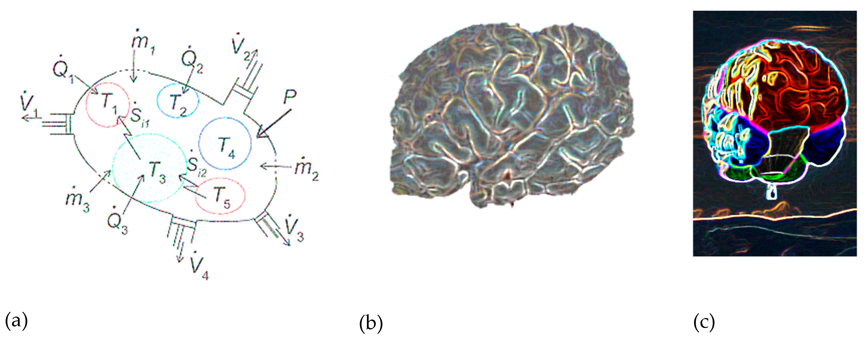

Table 1.
MEPR Validations across various types of studies.
| Characteristics | Relation | Measurement range and MEPR assessment | MEPR validations and assessments. |
| Energy Conservation | Bird Angle for V formation flights of Canadian Geese (5) | The observed V angle is ~ (110-130degrees for a small flock of Canadian geese (05, 06, 107). See Table 2. | The angel for the V formation = 2.tan-1 (Wingspan/Length). The median length/wingspan for Canadian Gesse, based on bird dimensions shown in Table 2 below, with MEPR analysis (5) is: 113-116 degrees. |
| Physical Constants | Diffusion Constants (62) |
Pb-0.01 wt% Sn Experimental: 1.656 x 10⁻⁹ m2/s From MEPR: (2.3 – 4.619) x 10-9 m2/s |
Pb-15 wt% % Sn Experimental: 1.656 x 10⁻⁹ m2/s From MEPR: (1-67 – 73.54) x 10-9 m2/s (the lower value corresponds to a modified partition coefficient. |
| Bifurcations | Dilute Alloys. Critical tipping point predictions. | Plane Front to Non-faceted Perturbations. The symbols are defined in [47,61,62,476] |
Plane front to Faceted Perturbations ηG is equal to one, and the highest density planes are oriented for growth (4) |
| Climate Sciences | Upward velocity is measured for non-equilibrium thunderclouds that can produce rain (44). | Recorded measurements are to 10 m/s for cumulonimbus clouds (reported in [44]. | MEPR calculated: Depends on For thickness between 1 km and 24 km, the velocity can be 6 m/s to 11 km/s |
Disclaimer/Publisher’s Note: The statements, opinions and data contained in all publications are solely those of the individual author(s) and contributor(s) and not of MDPI and/or the editor(s). MDPI and/or the editor(s) disclaim responsibility for any injury to people or property resulting from any ideas, methods, instructions or products referred to in the content. |
© 2025 by the authors. Licensee MDPI, Basel, Switzerland. This article is an open access article distributed under the terms and conditions of the Creative Commons Attribution (CC BY) license (http://creativecommons.org/licenses/by/4.0/).
Copyright: This open access article is published under a Creative Commons CC BY 4.0 license, which permit the free download, distribution, and reuse, provided that the author and preprint are cited in any reuse.


