
Submitted:
19 November 2025
Posted:
20 November 2025
You are already at the latest version
Abstract
Shape-restricted regression provides a framework for estimating an unknown regression function $f_0: \Omega \subset \mathbb{R}^d \rightarrow \mathbb{R}$ from noisy observations \((\boldsymbol{X}_1, Y_1), \ldots, (\boldsymbol{X}_n, Y_n)\) when no explicit functional relationship between $\boldsymbol{X}$ and $Y$ is known, but $f_0$ is assumed to satisfy structural constraints such as monotonicity or convexity. In this work, we focus on these two shape constraints (monotonicity and convexity), and provide a review on the isotonic regression estimator, which is a least squares estimator under monotonicity, and the convex regression estimator, which is a least squares estimator under convexity. We review existing literature with an emphasis on the following key aspects: quadratic programming formulations of isotonic and convex regression, statistical properties of these estimators, efficient computational algorithms for computing them, their practical applications, and current challenges. Finally, we conclude with a discussion of open challenges and possible directions for future research.
Keywords:
nonparametric regression
; shape-restricted regression
; convex regression
; isotonic regression
1. Introduction
One of the central problems in statistics and simulation is to estimate an unknown function from noisy observations , where we assume
for , is a closed convex subset of , and the ’s are independent and identically distributed (iid) mean zero random variables with finite variance . This type of problem arises in many settings. For instance, may represent a parameter in a stochastic system, such as the service rate of a single-server queue, and a performance metric, such as the steady-state mean waiting time in that single server queue when the service rate equals .
In many applications, there is no-closed form formula for . In such a case, a practical approach is to simulate the system at selected design points , obtain simulated outputs as estimates of , respectively, and use the data to approximate : This is a typical regression problem. The problem becomes challenging when it is impossible to place the relationship into a simple parametric form. However, when is known to satisfy certain structural properties such as monotonicity or convexity, shape-restricted regression offers powerful estimators.
Given such prior shape information, a natural estimator of fits a function f with such a shape characterization to the data set and solves
where is the class of functions satisfying the assumed shape constraint. For example, if is known to be nondecreasing, we can set , where
On the other hand, if is known to be convex, then we can set , where
Throughout this paper, we will focus on these two types of problems, the one with which leads to isotonic regression and the other with which leads to convex regression.
One of the first questions that arises is how to compute the solution to (1) numerically when or . Below, we describe how the solution to (1) can be obtained by solving quadratic programming (QP) problems.
1.1. QP Formulation for Isotonic Regression When
When is nondecreasing in , as when price increases with demand, we estimate by fitting a nondecreasing function f that minimizes squared errors . Writing and assuming the design is ordered so , the existence of a nondecreasing fit through is equivalent to . Thus, the estimator solves the following quadratic programming (QP) problem:
Let be a solution to (2). Any nondecreasing function interpolating defines the isotonic regression estimator and we will denote it by ; see, for example, Brunk [1].
1.2. QP Formulation for Convex Regression When
Suppose instead is convex. Writing and assuming the design is ordered so , a convex fit through exists if and only if
Hence, the least-squares convex fit solves
Let be a solution to (3). Any convex function interpolating is a convex regression estimator and we will denote it by ; see, for example, Hildreth [2].
1.3. Key Questions
Isotonic and convex regression are nonparametric methods that avoid any bandwidth or tuning parameters in their basic form yet enjoy strong theoretical guarantees. In particular, as , these estimators converge to under standard conditions even when the noise variance does not decrease. This is due to the fact that the estimators are required to satisfy the shape constraints, and hence, just adding more and more data points enforces the estimators to converge to the true underlying function.
Over the past seven decades, extensive work was done to study their statistical properties, computational algorithms, and practical applications. This paper reviews the literature on these topics and highlights unresolved questions. We focus on answering the following questions:
- How can the estimator be computed numerically from data ?
- What are its statistical properties?
- Are there efficient algorithms that are tailored to the computation of the isotonic or convex regression estimators?
- What applications benefit most from these approaches?
- What are its limitations, and how can we overcome them?
- What are the challenges that still lie in this field?
1.4. Organization of This Paper
The remainder of the paper is organized as follows. Section 2 reviews how the isotonic and convex regression estimators can be computed via QP problems. Section 3 focuses on isotonic regression while Section 4 examines convex regression in greater detail. Section 5 includes some conclusions while Section 6 discusses open challenges and future research directions.
1.5. Notation and Definitions
Throughout this paper, we view vectors as columns and write to denote the transpose of a vector . For , we write its ith component as , so . We define and .
For any convex set and a convex function , a vector is said to be a subgradient of g at if for all . We denote a subgradient of f at by . The set of all subgradients of g at is called the subdifferential of g at , denoted by . When a function is differentiable at , we denote its gradient at by . When is differentiable, we denote its gradient at by .
For a sequence of random variables and a sequence of positive real numbers , we say as if, for any , there exist constants c and such that for all .
For any sequences of real numbers and , if there exists a positive real number M and a real number such that for all .
For any sequence of random variables and any random variable B, means converges in distribution to B, or converges weakly to B as .
2. The Basic QP Formulation
In this section, we describe how the isotonic and convex regression estimators can be found by solving QP problems. Since there are many efficient algorithms for solving QP problems, expressing the isotonic and convex regression estimators as solutions to QP problems offers a basic way to compute them numerically. In , (2) and (3) already provide QP formulations for the isotonic and convex regression estimators, respectively. We now present multivariate analogues.
2.1. Isotonic Regression When
The main challenge in finding the QP formulation for the multivariate isotonic regression estimator is how to express the monotonicity of a multivariate function in linear inequalities as in the constraints of (2). We will define a non-decreasing function g as follows:
for and in , where indicates for .
Using this definition, the nondecreasing function with the minimum sum of squared errors can be found by solving the following QP problem in decision variables :
Let be a solution to (4). Any nondecreasing function interpolating can serve as the isotonic regression estimator and we will denote it by
2.2. Convex Regression When
Again, the key question is how to express the existence of a convex function going through as a set of linear constraints. One should notice that there exists a convex function passing through if and only if there exist satisfying
see page 338 of Boyd and Vandenberghe [3]. Here, serves as a subgradient of the convex function f at . Hence, a convex function with the least squares can be found by solving the following QP problem in decision variables and :
Let be a solution to (5). Any convex function going through can serve as the convex regression estimator in the multidimensional case. However, to remove any ambiguity, we will define the convex regression estimator as follows:
for .
3. Isotonic Regression
In this section, we review statistical properties, interesting applications, and some challenges of isotonic regression estimator. We also review some algorithms for computing the isotonic regression estimator numerically.
3.1. Statistical Properties
3.1.1. Univariate Case
The isotonic regression estimator in one and multiple dimensions was first introduced by Brunk [1]. In one dimension, Brunk [4] established its strong consistency. More specifically, Brunk [4] proved that if , for any and ,
as with probability one.
Brunk [5] established the asymptotic distribution theory for the isotonic regression estimator when . Brunk [5] proved that when ,
as , where is the two-sided Brownian motion starting from 0.
The -risk of the isotonic regression estimator, defined by
is proven to have the following bound
where is the total variation of and is a universal constant. Meyer and Woodroofe [6] proved (6) under the assumption that the ’s are normally distributed, and Zhang [7] proved (6) under a more general assumption that the ’s are iid with mean zero and variance .
3.1.2. Multivariate Case
In multiple dimensions, Lim [8] established the strong consistency. Corollary 3.1 of Lim [8] proved that when , for any
as with probability one.
Lim [8] also established the rate of convergence and proved that
where the expectation is taken with respect to , has the same distribution as the ’s, and , a variant of the isotonic regression estimator, minimizes the sum of squared errors over all nondecreasing functions f satisfying for some pre-set constant C for all .
Bagchi and Dhar [9] derived the pointwise limit distribution of the isotonic regression estimator in multiple dimensions. In particular, Bagchi and Dhar [9] proved
as for some non-degenerate limit distribution H.
Han et al. [10] showed that the -risk of a multivariate isotonic regression estimator is bounded by a constant multiple of for all .
3.2. Computational Algorithms
Formulations (2) and (3) are QPs with linear constraints, and hence, can be solved by off-the-shelf solvers such as CVX, CPLEX, or MOSEK. However, there exist algorithms tailored to the specific setting of the isotonic regression estimator. In , Barlow et al. [11] discussed a graphical procedure to compute the isotonic regression estimator by identifying it as the greatest common minorant for a cumulative sum diagram, and proposed a tabular procedure called the pool-adjacent-violators (PAV) algorithm. PAV algorithm computes the isotonic regression estimator in steps. Various modifications of the PAV algorithm have been proposed in the literature; see Brunk [1], Mukerjee [12], Mammen [13], Friedman and Tibshirani [14], Ramsay [15], or Hall and Huang [16], among many others.
However, for regression functions of more than one variable, the problem of computing isotonic regression estimators is substantially more difficult, and good algorithms are not available except for special cases. Most of the literature deals with algorithms for multivariate isotonic regression on a grid (see Gebhardt [17], Dykstra and Robertson [18], Lee [19], or Qian and Eddy [20], among others), but little work has been done for the case of random design.
3.3. Applications
In many applications of economics, operations research, biology, and medical sciences, monotonicity is often assumed to be hold or is mathematically proven to hold. For example, in economics, economists often assume the downward slope of the demand as a function of the price. Also, monotonicity applies to indirect utility, expenditure production, profit, and cost functions; see Gallant and Golub [21], Matzkin [22], or Aït-Sahalia and Duarte [23], among many others. In operations research, the steady-state mean waiting time of a customer in a single-server queue is proven to be nonincreasing as a function of the service rate; see Weber [24]. In biology, the weight or height of growing objects over time are known to be nondecreasing over time. In medical sciences, the blood pressure is believed to be a monotone function of the use of tobacco and the body weight (see Moolchan et al. [25]) and the probability of contracting a cancer depends monotonically on certain factors such as smoking frequency, drinking frequency, and weight.
3.4. Challenges
Two common issues in the isotonic regression estimator are (i) non-smoothness (piecewise constant fits) and (ii) boundary overfitting (“spiking”). Figure 1 displays an instance of the true regression function , the ’s, and the isotonic regression estimator. The isotonic regression estimator in Figure 1 is piecewise constant, and hence, non-smooth. Also, it overfits near the boundary of its domain.
3.4.1. Non-Smoothness of Isotonic Regression
To overcome the non-smoothness of the isotonic regression estimator, several researchers proposed variants of the isotonic regression estimator. Ramsay [15] considered the univariate case and proposed estimating as a nonnegative linear combination of the I-splines given the knot sequence in . The I-splines are monotone by definition, so the corresponding estimator is guaranteed to be monotone. This method, however, can be sensitive to the number and placement of knots and the order of the I-splines. Mammen [13] also considered the univariate case and proposed computing the isotonic regression estimator and then making it smooth by applying kernel regression. He and Shi [26] considered the univariate case and proposed fitting normalized B-splines to the data set given the knot sequence in . This method is also sensitive to the number and placement of the knots. See Mammen and Thomas-Agnan [27] and Meyer [28] for other approaches in the univariate case.
In multiple dimensions, Dette and Scheder [29] proposed a procedure that smooths the data points using a kernel-type method and then applies an isotonization step to each coordinate so that the resulting estimate maintains the monotonicity in each coordinate.
3.4.2. Overfitting of Isotonic Regression
The isotonic regression estimator is known to be inconsistent at boundaries; this is called the “spiking” problem. See Figure 1 for an illustration of this phenomenon. Proposition 1 of Lim [30] proved that when , does not converge to in probability as . One popular remedy for this is using a penalized isotonic regression estimator, which minimizes the sum of squared errors plus a penalty term over all monotone functions. A penalized isotonic regression estimator can be expressed as the solution to the following problem:
where is a smoothing parameter and is a penalty term. Wu et al. [31] considered the case where equals the range of f divided by n. They proved that when , the solution to (7) (which is often referred to as the “bounded isotonic regression”) evaluated at converges to in probability as . This proves that the bounded isotonic regression estimator is consistent at the boundary unlike the traditional isotonic regression estimator. Wu et al. [31] also proved similar results for the case when the covariates are on a grid. Luss and Rosset [32] proposed an algorithm for solving the bounded isotonic regression for the multivariate case. On the other hand, Lim [30] considered the case where for the case and established the strong consistency of the corresponding estimator at , thereby proving that the estimator is consistent at the boundary of . Lim [30] also computed the convergence rate of for the proposed estimator.
Even though several approaches are proposed for the case, limited work is available for the multivariate case. Isotonic regression estimator’s overfitting problem in the case is a good research topic for future.
4. Convex Regression
In this section, we review statistical properties, interesting applications, and some challenges of convex regression estimator. We also review some algorithms for computing the convex regression estimator numerically.
4.1. Statistical Properties
4.1.1. Univariate Case
The convex regression estimator, along with its QP formulation in (3), was first introduced by Hildreth [2] for the case. Hanson and Pledger [33] established strong consistency on compact subsets of . They proved that, if , for any and ,
as with probability one.
Results on rates of convergence were obtained by Mammen [34] and Groeneboom et al. [35]. In particular, Mammen [34] showed that at any interior point ,
as , provided that the second derivative of at does not vanish.
Groeneboom et al. [35] identified the limiting distribution of at a fixed point . Groeneboom et al. [35] proved that if the errors are iid sub-Gaussian with mean zero and ,
where denotes the greatest convex minorant (i.e., envelope) of integrated Brownian motion with quartic drift , and is its second derivative at 0. The envelope can be viewed as a cubic curve lying above and touching the integrated Brownian motion .
More recently, Chatterjee [36] derived an upper bound on the -risk of the convex regression estimator. Under the assumption of iid Gaussian errors with mean zero, they showed that
for all , where C is a constant.
4.1.2. Multivariate Case
The multivariate convex regression estimator and its QP formulation in (5) were first introduced by Allon et al. [37]. Strong consistency over any compact subset of the interior of was established by Seijo and Sen [38] and Lim and Glynn [39]. Seijo and Sen [38] proved that for any compact subset A of the interior of ,
as with probability one under some modest assumptions.
Rates of convergence were obtained by Lim [40]. In particular, Lim [40] considered a variant of the convex regression estimator, say , which minimizes the sum of squared errors over the set of convex functions f with subgradients bounded uniformly by a constant. Lim [40] showed that
as .
A bound on the global risk has been established by Han and Wellner [41] as follows:
as , where is the density function of and minimizes the sum of squared errors over the set of convex functions f bounded uniformly by a constant.
The limiting distribution of for an appropriate rate of convergence has not be established so far and this is still an open problem.
4.2. Computational Algorithms
In the univariate case, Dent [42] introduced a QP formulation of the convex regression estimator as in (3). Dykstra [43] developed an iterative algorithm to compute the convex regression estimator numerically. The procedure proposed by Dykstra [43] is guaranteed to converge to the convex regression estimator as the number of iterations approaches infinity. For other algorithms for solving the QP in (3), see Wu [44] and Fraser and Massam [45].
For the multivariate setting, Allon et al. [37] first presented the QP formulation given in (5). However, this formulation requires linear constraints, which limits its applicability to data sets of only a few hundred observations under current computational capabilities. To address this, Mazumder et al. [46] proposed an algorithm based on the augmented Lagrangian method. Their approach was able to solve (5) for and within a few seconds.
To mitigate the computational burden, several authors (Magnani and Boyd [47]; Aguilera et al. [48]; Hannah and Dunson [49]) proposed approximating the convex regression estimator by the maximum of a small set of hyperplanes. Specifically, they solved the optimization problem
where defines a hyperplane and is the set of positive integers. Their estimator is then given by the maximum over these hyperplanes:
More recently, to handle larger data sets, Bertsimas and Mundru [50] introduced a penalized convex regression estimator defined as the solution to the following QP problem in decision variables and :
where is a smoothing parameter. They proposed a cutting-plane algorithm for solving (8) and reported that it can handle data sets with and within minutes.
Another strategy to alleviate the computational burden of the convex regression estimator is to reformulate the problem as a linear programming (LP) problem rather than a quadratic program. Luo and Lim [51] proposed estimating the convex function that minimizes the sum of absolute deviations (instead of the sum of squared errors). The resulting estimator can be obtained by solving the following LP problem in decision variables and :
Luo and Lim [51] further showed that the corresponding estimator converges a.s. to the true function as over any compact subset of the interior of .
4.3. Applications
Convexity and concavity play an important role across various fields, including economics and operations research. In economics, for instance, it is common to assume diminishing marginal productivity with respect to input resources, which implies that the production function is concave in its inputs (Allon et al. [37]). Also, demand (Varian [52]) and utility (Varian [53]) functions are often assumed to be convex/concave. In operations research, the steady-state waiting time in a single-server queue has been shown to be convex in the service rate; see, for example, Weber [24]. An additional example is provided in Demetriou and Tzitziris [54], where infant mortality rates are modeled as exhibiting increasing returns with respect to the gross domestic product (GDP) per capita, leading to the assumption that the infant mortality function is convex in GDP per capita. For further applications of convex regression, see Johnson and Jiang [55].
4.4. Challenges
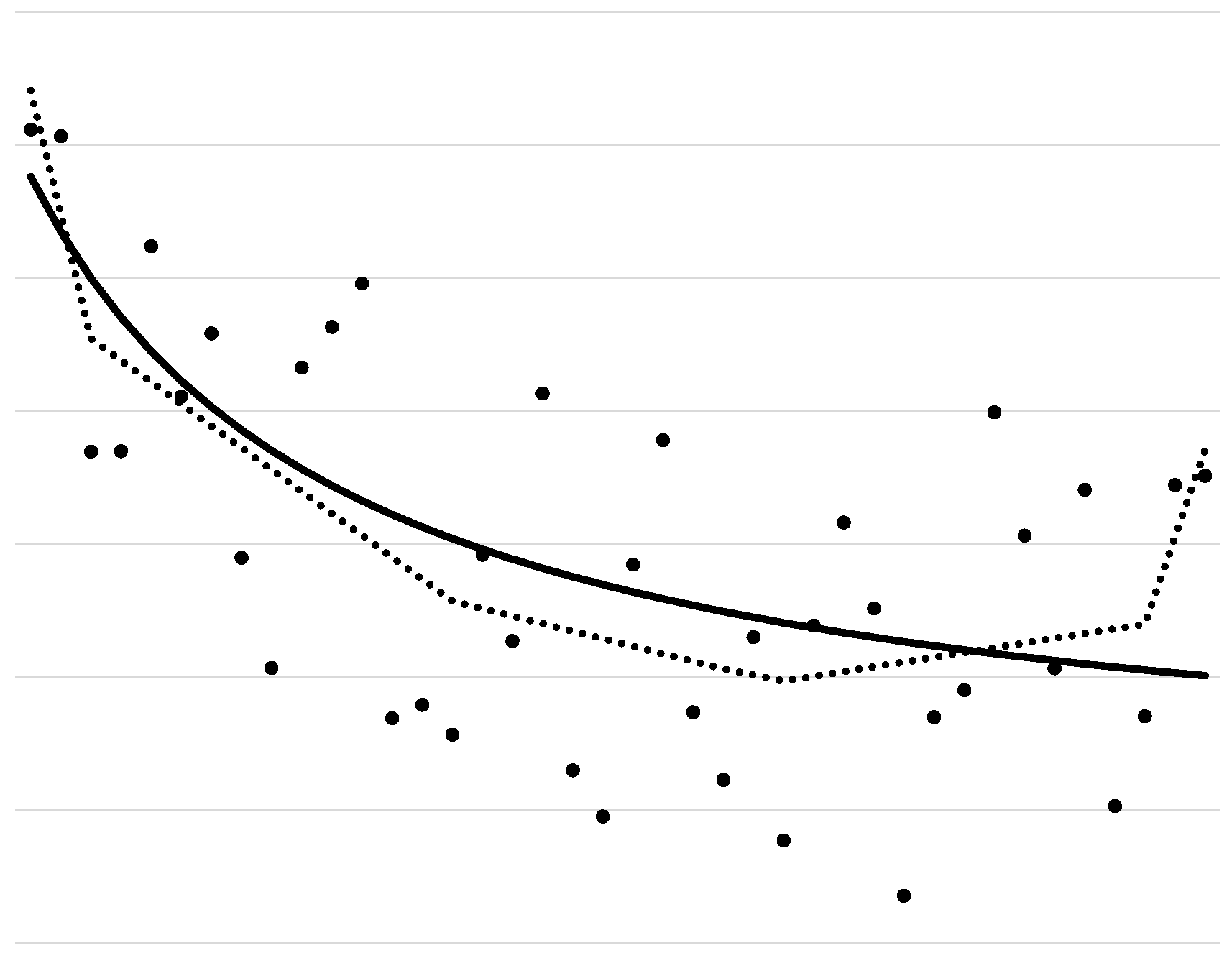
The convex regression estimator faces two primary limitations: (i) non-smoothness (piecewise linear fits) and (ii) overfitting near the boundary of its domain (“spiking”). Figure 2 illustrates these issues by displaying the true regression function , the observed data , and the convex regression estimator. As shown, the convex regression estimator is piecewise linear and therefore non-smooth. It also exhibits boundary overfitting.
4.4.1. Non-Smoothness of Convex Regression
In the univariate setting, several approaches have been proposed to address the lack of smoothness. Mammen and Thomas-Agnan [27] developed a two-step procedure in which the data are first smoothed using nonparametric smoothing methods, followed by convex regression applied to the smoothed values. Alternatively, Aït-Sahalia and Duarte [23] suggested first estimating the convex regression estimator and then applying local polynomial smoothing to the estimator. Birke and Dette [56] proposed a different strategy: smoothing the data with a nonparametric method such as the kernel, local polynomial, series, or spline methods, computing its derivative, applying isotonic regression to the derivative, and integrating to obtain a convex estimator. Other methods for the univariate case are discussed in Du et al. [57].
In the multivariate case, Mazumder et al. [46] constructed a smooth approximation to the convex regression estimator that remains uniformly close to the original estimator.
4.4.2. Overfitting of Convex Regression
As with isotonic regression, convex regression tends to overfit near domain boundaries, often producing extremely large subgradients and inconsistent estimates of near the boundary. For , Ghosal and Sen [58] showed that the convex regression estimator fails to converge in probability to the true value at boundary points and that its subgradients at the boundary are unbounded in probability as .
A common strategy to mitigate overfitting is to constrain the subgradients. Lim [40] proposed bounding the norm of the subgradients, imposing for all i for some fixed to the constraints of (5). Instead, Mazumder et al. [46] added to the constraints of (5).
Another widely used approach is penalization, which adds a penalty term to the objective function of (1). Chen et al. [59] and Bertsimas and Mundru [50] studied a penalized multivariate convex regression estimator defined as the solution to the following QP problem in decision variables :
Lim [60] generalized this idea and proposed the following three alternative approaches:
for some smoothing parameter and constants , where is a penalty term measuring the overall magnitude of the subgradient of f.
In particular, Lim [60] considered the case where
and represents the partial derivative of f with respect to the ith component of . Lim [60] established the uniform strong consistency of and and their derivatives. Specifically, she showed that
and
as with probability one. Analogous results were shown for . These results confirm that penalization successfully eliminates boundary overfitting.
Finally, Lim [60] derived convergence rates for and . For , she proved
as , and for , she established
as .
5. Conclusions
Shape-restricted regression offers a way to incorporate qualitative information, such as monotonicity and convexity, into nonparametric function estimation without relying on bandwidths or other tuning parameters. In this review, we have focused on the isotonic and convex regression, and have highlighted how they arise naturally in areas such as statistics, economics, and operations research. By expressing these estimators as solutions to QP problems, we established a unified optimization framework that facilitates their numerical computation.
On the theoretical side, a substantial body of work has established strong consistency, convergence rates, and risk bounds for isotonic and convex regression. At the same time, the literature has identified important limitations of these estimators, including their inherent non-smoothness and boundary overfitting (“spiking”), which can severely distort behavior near the edges of the design space.
These shortcomings have motivated a variety of methodological extensions. For isotonic regression, smoothing via splines, kernel methods, and other post- or pre-processing steps, as well as penalization schemes such as bounded isotonic regression, have been proposed to improve smoothness and boundary behavior. For convex regression, bounding or penalizing subgradients has emerged as an effective strategy to control overfitting while preserving convexity.
6. Future Directions
This section outlines several open problems that, in our view, remain both important and underexplored. Although some of these topics have appeared in prior work, they call for substantially deeper investigation.
6.1. Problem 1. Scalable Algorithms for Large-Scale Data
Modern applications frequently involve data sets with millions of observations. For example, when a hiring manager receives an application through LinkedIn, the platform is expected to infer the applicant’s seniority level using massive amounts of historical data. Problems of this nature essentially reduce to isotonic regression with millions of data points. At present, no computational algorithm exists that can efficiently compute the isotonic regression estimator at such a scale. In the era of “Big Data,” there is an urgent need for scalable algorithms capable of handling large-scale isotonic and convex regression problems.
6.2. Problem 2. Algorithms for Multivariate Isotonic Regression
In the multivariate setting, efficient algorithms for isotonic regression under random designs remain largely unavailable.
6.3. Problem 3. Pointwise Limit Distribution of Multivariate Convex Regression
Although most major theoretical properties of shape-restricted estimators have been established over the past seven decades, one central question remains open: the pointwise limiting distribution of the multivariate convex regression estimator. Specifically, it is unknown whether
converges weakly to a non-degenerate limit for some appropriate normalization , and if so, what the form of that limit should be. Resolving this would close one of the most significant remaining theoretical gaps in convex regression.
6.4. Problem 4. Incorporating Smoothness into Shape-restricted Regression in Multiple Dimensions
Although several studies have explored ways to address the inherent non-smoothness of shape-restricted regression, existing methods remain preliminary. More effective techniques are needed for incorporating smoothness into multivariate isotonic and convex regression estimators.
6.5. Problem 5. Overfitting in Isotonic and Convex Regression
Only a handful of methods exist to mitigate overfitting in isotonic and convex regression. The most common strategies involve (i) adding a penalty term to the least squares objective function in (1), or (ii) imposing a hard bound on the subgradients (in the convex regression case). Both approaches introduce tuning parameters such as the smoothing constants or gradient bounds that must be chosen in practice, often arbitrarily or in a data-dependent ad-hoc manner. This raises two fundamental questions: How can these parameters be optimally determined? Are there alternative strategies for preventing overfitting without relying on externally imposed parameters?
6.6. Problem 6. Theory for Penalized Isotonic and Convex Regression
There remains substantial scope for advancing the theoretical foundations of penalized isotonic and convex regression. For penalized isotonic regression, most existing results address only the univariate case; extending these insights to higher dimensions remains open. For penalized convex regression, many fundamental questions about its theoretical behavior are still unresolved.
Funding
This research received no external funding.
Conflicts of Interest
The author declares no conflicts of interest.
References
- Brunk, H.D. Maximum likelihood estimates of monotone parameters. Ann. Math. Stat. 1955, 26, 607–616. [Google Scholar] [CrossRef]
- Hildreth, C. Point estimates of ordinates of concave functions. J. Amer. Statist. Assoc. 1954, 49, 598–619. [Google Scholar] [CrossRef]
- Boyd, S.; Vandenberghe, L. Convex Optimization; Cambridge University Press: Cambridge, UK, 2004. [Google Scholar]
- Brunk, H.D. On the estimation of parameters restricted by inequalities. Ann. Math. Statist. 1958, 29, 437–454. [Google Scholar] [CrossRef]
- Brunk, H.D. Estimation of isotonic regression. In Nonparametric Techniques in Statistical Inference; Cambridge Univ. Press: New York, 1970; pp. 177–195. [Google Scholar]
- Meyer, M.; Woodroofe, M. On the degrees of freedom in shape-restricted regression. Ann. Statist. 2000, 28, 1083–1104. [Google Scholar] [CrossRef]
- Zhang, C.H. Risk bounds in isotornic regression. Ann. Statist. 2002, 30, 528–555. [Google Scholar] [CrossRef]
- Lim, E. The Limiting Behavior of Isotonic and Convex Regression Estimators When The Model Is Misspecified. Electron. J. Stat. 2020, 14, 2053–2097. [Google Scholar] [CrossRef]
- Bagchi, P.; Dhar, S.S. A study on the least squares estimator of multivariate isotonic regression function. Scand. J. Stat. 2020, 47, 1192–1221. [Google Scholar] [CrossRef]
- Han, Q.; Wang, T.; Chatterjee, S.; Samworth, R.J. Isotonic Regression in General Dimensions. Ann. Statist. 2019, 47, 2440–2471. [Google Scholar] [CrossRef]
- Barlow, R.E.; Bartholomew, R.J.; Bremner, J.M.; Brunk, H.D. Statistical Inference under Order Restrictions; Wiley: New York, 1972. [Google Scholar]
- Mukerjee, H. Monotone nonparametric regression. Ann. Statist. 1988, 16, 741–750. [Google Scholar] [CrossRef]
- Mammen, E. Estimating a smooth monotone regression function. Ann. Statist. 1991, 19, 724–740. [Google Scholar] [CrossRef]
- Friedman, J.; Tibshirani, R. The monotone smoothing of scatterplots. Technometrics 1984, 26, 243–250. [Google Scholar] [CrossRef]
- Ramsay, J.O. Monotone regression splines in action. Statist. Sci. 1988, 3, 425–461. [Google Scholar] [CrossRef]
- Hall, P.; Huang, L.S. Nonparametric kernel regression subject to monotonicity constraints. Ann. Statist. 2001, 29, 624–647. [Google Scholar] [CrossRef]
- Gebhardt, F. An algorithm for monotone regression with one or more independent variables. Biometrika 1970, 57, 263–271. [Google Scholar] [CrossRef]
- Dykstra, R.L.; Robertson, T. An algorithm for isotonic regression for two or more independent variables. Ann. Statist. 1982, 10, 708–716. [Google Scholar] [CrossRef]
- Lee, C.I.C. The min-max algorithm and isotonic regression. Ann. Statist. 1983, 11, 467–477. [Google Scholar] [CrossRef]
- Qian, S.; Eddy, W.F. An algorithm for isotonic regression on ordered rectangular grids. J. Comput. Graph. Statist. 1996, 5, 225–235. [Google Scholar] [CrossRef]
- Gallant, A.; Golub, G.H. Imposing curvature restrictions on flexible functional forms. Journal of Economics 1984, 26, 295–321. [Google Scholar] [CrossRef]
- Matzkin, R.L. Restrictions of economic theory in nonparametric methods. In Handbook of Econometrics Vol IV; North-Holland: Amsterdam, 1994; pp. 2523–2558. [Google Scholar]
- Aït-Sahalia, Y.; Duarte, J. Nonparametric option pricing under shape restrictions. J. Econometrics 2003, 116, 9–47. [Google Scholar] [CrossRef]
- Weber, R.R. A note on waiting times in single server queues. Oper. Res. 1983, 31, 950–951. [Google Scholar] [CrossRef]
- Moolchan, E.T.; Hudson, D.L.; Schroeder, J.R.; Sehnert, S.S. Heart rate and blood pressure responses to tobacco smoking among African-American adolescents. J. Natl. Med. Assoc. 2004, 96, 767. [Google Scholar] [PubMed]
- He, X.; Shi, P. Monotone B-spline smoothing. J. Amer. Statist. Assoc. 1998, 93, 643–650. [Google Scholar] [CrossRef]
- Mammen, E.; Thomas-Agnan, C. Smoothing splines and shapre restrictions. Scand. J. Stat. 1999, 26, 239–252. [Google Scholar] [CrossRef]
- Meyer, M.C. Inference using shape-restricted regression splines. Ann. Statist. 2008, 2, 1013–1033. [Google Scholar] [CrossRef]
- Dette, H.; Scheder, R. Strictly Monotone and Smooth Nonparametric Regression for Two Or More Variables. Canad. J. Statist. 2006, 34, 535–561. [Google Scholar] [CrossRef]
- Lim, E. An estimator for isotonic regression with boundary consistency. Statist. Probab. Lett. 2025, 226, 110513. [Google Scholar] [CrossRef]
- Wu, J.; Meyer, M.C.; Opsomer, J.D. Penalized isotonic regression. J. Statist. Plann. Inference 2015, 161, 12–24. [Google Scholar] [CrossRef]
- Luss, R.; Rosset, S. Bounded isotonic regression. Electron. J. Statist. 2017, 11, 4488–4514. [Google Scholar] [CrossRef]
- Hanson, D.L.; Pledger, G. Consistency in concave regression. Ann. Statist. 1976, 4, 1038–1050. [Google Scholar] [CrossRef]
- Mammen, E. Nonparametric regression under qualitative smoothness assumptions. Ann. Statist. 1991, 19, 741–759. [Google Scholar] [CrossRef]
- Groeneboom, P.; Jongbloed, G.; Wellner, J.A. Estimation of a convex function: Characterizations and Asymptotic Theory. Ann. Statist. 2001, 29, 1653–1698. [Google Scholar] [CrossRef]
- Chatterjee, S. An improved global risk bound in concave regression. Electron. J. Stat. 2016, 10, 1608–1629. [Google Scholar] [CrossRef]
- Allon, G.; Beenstock, M.; Hackman, S.; Passy, U.; Shapiro, A. Nonparametric estimatrion of concave production technologies by entropy. J. Appl. Econometrics 2007, 22, 795–816. [Google Scholar] [CrossRef]
- Seijo, E.; Sen, B. Nonparametric least squares estimation of a multivariate convex regression function. Ann. Statist. 2011, 39, 1633–1657. [Google Scholar] [CrossRef]
- Lim, E.; Glynn, P.W. Consistency of Multi-dmentional Convex Regression. Oper. Res. 2012, 60, 196–208. [Google Scholar] [CrossRef]
- Lim, E. On convergence rates of convex regression in multiple dimensions. INFORMS J. Comput. 2014, 26, 616–628. [Google Scholar] [CrossRef]
- Han, Q.; Wellner, J.A. Multivariate convex regression: Global risk bounds and adaptation. https://arxiv.org/abs/1601.06844, 2016. arXiv preprint.
- Dent, W. A note on least squares fitting of function constrained to be either non-negative, nondecreasing, or convex. Manag. Sci. 1973, 20, 130–132. [Google Scholar] [CrossRef]
- Dykstra, R.L. An algorithm for restricted least squares regression. J. Am. Stat. Assoc. 1983, 78, 837–842. [Google Scholar] [CrossRef]
- Wu, C.F. Some algorithms for concave and isotonic regression. TIMS Studies in Management Science 1982, 19, 105–116. [Google Scholar]
- Fraser, D.A.S.; Massam, H. A mixed primal-dual bases algorithm for regression under inequality constraints. Application to concave regression. Scand. J. Stat. 1989, 16, 65–74. [Google Scholar]
- Mazumder, R.; Iyengar, A.C.G.; Sen, B. A Computational Framework for Multivariate Convex Regression and Its Variants. J. Am. Stat. Assoc. 2019, 114, 318–331. [Google Scholar] [CrossRef]
- Magnani, A.; Boyd, S. Convex piecewise-linear fitting. Optim. Eng. 2009, 10, 1–17. [Google Scholar] [CrossRef]
- Aguilera, N.; Forzani, L.; Morin, P. On uniform consistent estimators for convex regression. J. Nonparametr. Stat. 2011, 23, 897–908. [Google Scholar] [CrossRef]
- Hannah, L.A.; Dunson, D.B. Multivariate Convex Regression with Adaptive Partitioning. J. Mach. Learn. Res. 2013, 14, 3261–3294. [Google Scholar]
- Bertsimas, D.; Mundru, N. Sparse Convex Regression. INFORMS J. Comput. 2021, 33, 262–279. [Google Scholar] [CrossRef]
- Luo, Y.; Lim, E. On consistency of absolute deviations estimators of convex functions. International Journal of Statistics and Probability 2016, 5, 1–18. [Google Scholar] [CrossRef]
- Varian, H.R. The nonparametric approach to demand analysis. Econometrica 1982, 50, 945–973. [Google Scholar] [CrossRef]
- Varian, H.R. The nonparametric approach to production analysis. Econometrica 1984, 52, 579–597. [Google Scholar] [CrossRef]
- Demetriou, I.; Tzitziris, P. Infant mortality and economic growth: Modeling by increasing returns and least squares. In Proceedings of the Proceedings of the World Congress on Engineering, 2017, Vol.
- Johnson, A.L.; Jiang, D.R. Shape Constraints in Economics and Operations Research. Statist. Sci. 2018, 33, 527–546. [Google Scholar] [CrossRef]
- Birke, M.; Dette, H. Estimating a convex function in nonparametric regression. Scand. J. Statist. 2007, 34, 384–404. [Google Scholar] [CrossRef]
- Du, P.; Parmeter, C.F.; Racine, J.S. Nonparametric kernel regression with multiple predictors and multiple shape constraints. Statist. Sinica 2013, 23, 1347–1371. [Google Scholar]
- Ghosal, P.; Sen, B. On univariate convex regression. Sankhya A 2017, 79, 215–253. [Google Scholar] [CrossRef]
- Chen, X.; Lin, Q.; Sen, B. On degrees of freedom of projection estimators with applications to multivariate nonparametric regression. J. Amer. Statist. Assoc. 2020, 115, 173–186. [Google Scholar] [CrossRef]
- Lim, E. Convex Regression with a Penalty. http://arxiv.org/abs/2509.19788, 2025. arXiv preprint.
Figure 1.
The solid line is , the circles are the values, and the dotted line is the isotonic regression estimator.
Figure 1.
The solid line is , the circles are the values, and the dotted line is the isotonic regression estimator.
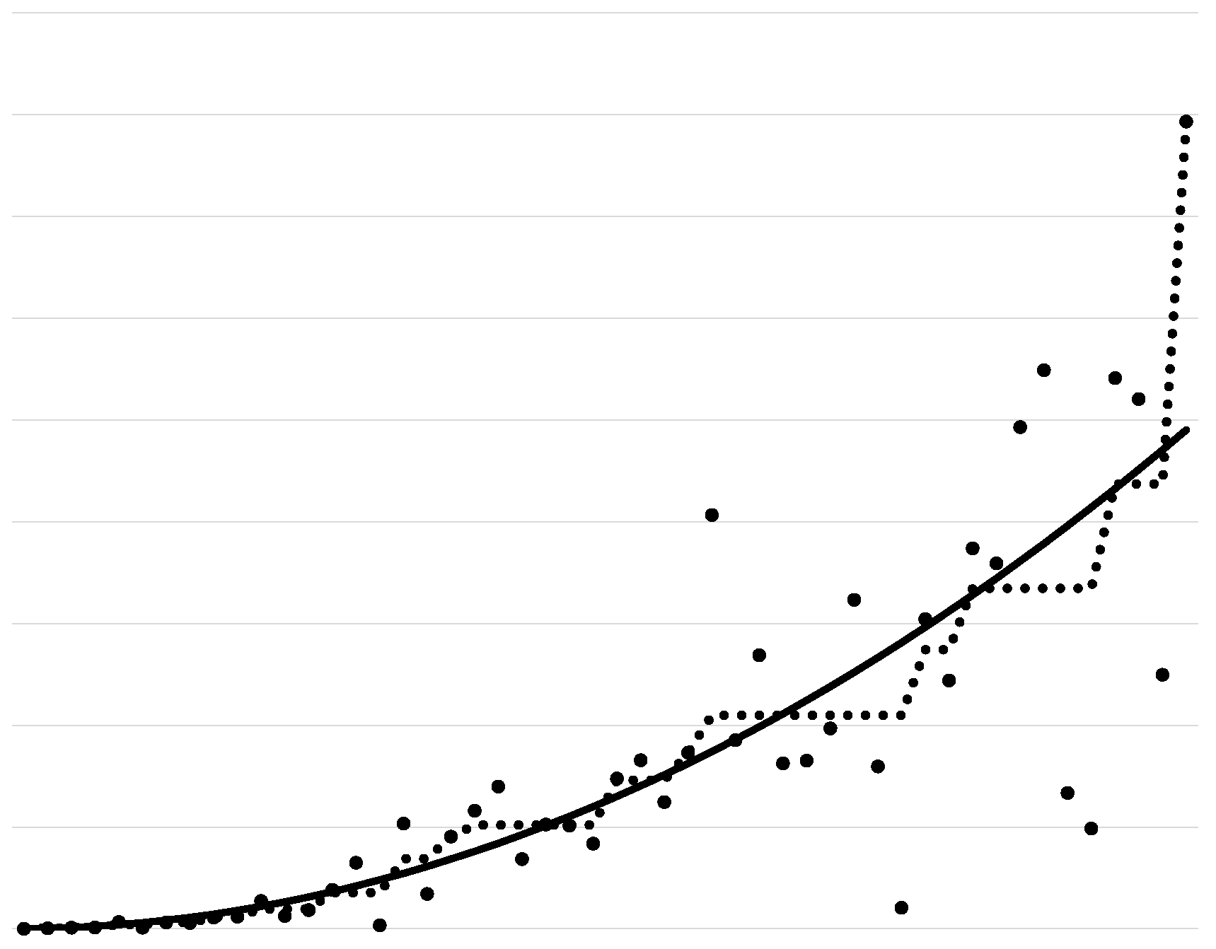
Figure 2.
The solid line represents , the circles denote the observed data , and the dotted line corresponds to the convex regression estimator.
Figure 2.
The solid line represents , the circles denote the observed data , and the dotted line corresponds to the convex regression estimator.
Disclaimer/Publisher’s Note: The statements, opinions and data contained in all publications are solely those of the individual author(s) and contributor(s) and not of MDPI and/or the editor(s). MDPI and/or the editor(s) disclaim responsibility for any injury to people or property resulting from any ideas, methods, instructions or products referred to in the content. |
© 2025 by the authors. Licensee MDPI, Basel, Switzerland. This article is an open access article distributed under the terms and conditions of the Creative Commons Attribution (CC BY) license (http://creativecommons.org/licenses/by/4.0/).
Copyright: This open access article is published under a Creative Commons CC BY 4.0 license, which permit the free download, distribution, and reuse, provided that the author and preprint are cited in any reuse.


