
Submitted:
19 November 2025
Posted:
20 November 2025
You are already at the latest version
Abstract
Earthquake prediction remains one of the central unsolved problems in geophysics, and ionospheric variability offers a promising yet debated window into the earthquake preparation process through lithosphere–atmosphere–ionosphere coupling. Progress has been hindered by methodological limitations in prior studies, including the use of inappropriate performance metrics for highly imbalanced seismic data, the reliance on geographically and temporally narrow data, and inclusion of inherent spatial or temporal features that artificially inflate model performance while preventing the discovery of genuine ionospheric precursors. To address these challenges, we introduce a global, temporally validated machine learning framework grounded in thirty-five years of ionospheric observations from thirty-seven stations. Our framework eliminates lookahead bias through strict temporal partitioning, evaluates precursor sensitivity through systematic relaxation of the Dobrovolsky radius, and applies ensemble feature selection that excludes spatial and temporal identifiers to prevent leakage and coincidence effects. Cross-regional validation shows that gradient boosting models yield the strongest classification skill, with a weighted F1 score of 77%, and that ionospheric parameters account for a substantial portion of earthquake magnitude variability. These findings provide quantitative support for LAIC processes while revealing the multivariate nature of seismic precursors. Our study demonstrates learnable, spatiotemporally invariant ionospheric precursors, though the 15.4% of undetected earthquakes indicates that ionospheric monitoring alone is insufficient for operational deployment and multimodal fusion with complementary precursor channels is required.
Keywords:
earthquake prediction
; ionospheric precursors
; machine learning
; LAIC
; spatiotemporal feature learning
; temporal validation
; cross-regional generalization
1. Introduction
Earthquakes represent one of the most destructive natural phenomena, posing a persistent threat to human life due to their unpredictable nature. Despite extensive geophysical monitoring, short-term earthquake prediction remains elusive [1], as seismic processes involve complex, nonlinear interactions within the Earth’s crust that defy straightforward forecasting. Among the proposed mechanisms, the Lithosphere-Atmosphere-Ionosphere Coupling (LAIC) model [2] describes a chain of interactions through which stress accumulation in the crust may modify atmospheric and ionospheric properties.
However, existing research predominantly relies on case studies of isolated events or limited datasets from few monitoring stations [3,4,5,6], often reporting high accuracy on small, imbalanced datasets without rigorous controls for data leakage or temporal validation, lacking the large-scale, cross-regional evidence required to distinguish true precursors from coincidental anomalies [7,8].
In this study we investigate whether ionospheric measurements, augmented by solar activity indices, serve as reliable precursors for earthquake occurrence and magnitude estimation. Our primary contribution is a comprehensive, multi-decadal dataset (1990–2025) from 37 global ionosonde stations and worldwide seismic catalogs, revealing robust spatiotemporally invariant patterns across diverse tectonic settings. We employ imbalance-aware metrics and strict temporal splitting to prevent data leakage, yielding credible performance estimates. Furthermore, we empirically validate the Dobrovolsky radius [9] through systematic relaxation and contraction testing, confirming its applicability for ionospheric precursor detection.
2. Theoretical Foundation: Lithosphere–Atmosphere–Ionosphere Coupling
The Lithosphere–Atmosphere–Ionosphere Coupling (LAIC) framework [2,10] provides the physical basis for seismo-ionospheric interactions, describing how pre-seismic processes in the crust can produce measurable ionospheric responses. The model identifies three principal coupling pathways operating on distinct temporal and physical scales.
Chemical channel: Progressive crustal stress enhances microfracturing and radon release [11,12]. Radon decay increases ion production in the boundary layer, modifies atmospheric conductivity, and perturbs the global electric circuit [13]. These electric field disturbances can map to ionospheric heights and alter plasma density hours to days before an earthquake. Numerous case studies report elevated radon emanation preceding seismic events [14,15].
Acoustic channel: Crustal deformation can excite acoustic–gravity waves (AGWs) that propagate upward and amplify in the rarefied atmosphere [16,17]. Upon reaching the ionosphere, AGWs modulate neutral dynamics, ion–neutral collisions, and vertical plasma transport, producing periodic electron density variations. This channel primarily governs short-timescale (minutes to hours) co-seismic and post-seismic disturbances [18,19], though pre-seismic AGW signatures have also been reported [20].
Electromagnetic channel: Stressed rocks can generate electromagnetic emissions through piezoelectric, electrokinetic, and defect-activated charge mechanisms [21,22]. These ULF–VLF fields may propagate to or interact with the ionosphere, where they can heat electrons, modify temperature anisotropy, and trigger plasma instabilities [23,24]. This pathway may operate throughout the preparation stage and thus provide some of the earliest signals.
In practice, these channels likely act concurrently, with their relative strengths depending on earthquake parameters, geological context, and ionospheric conditions [25]. Because our dataset includes both bottomside (foE, foF1) and topside (foF2, TEC) parameters, it is well suited to differentiating the layer-specific signatures expected from the chemical, acoustic, and electromagnetic coupling mechanisms.
3. Data
The possibility of ionospheric precursors to seismic events remains contentious due to conflicting observations and lack of accepted physical mechanisms [26,27,28]. Our previous work on Schumann resonance signals in the Greek region [29] attempted to move beyond isolated case studies of electromagnetic precursors toward a more holistic approach. Subsequently, our initial investigation of ionospheric precursors at Athens station (AT138) using statistical correlation and machine learning revealed marginally significant correlations but poor predictive performance (AUC ≈ 0.55, barely above random). This failure stems from limited sample size, regional ionospheric peculiarities, and noise from Athens’ exceptionally high seismic frequency causing overlapping precursor windows that mask event-specific signals [1,30]. Recognizing these limitations, we transition here to a global-scale investigation of ionospheric precursors, leveraging spatial and temporal diversity across 37 stations to overcome the regional confounds that hindered localized analysis.
3.1. Rationale for Multi-Regional Analysis
Single-station studies face inherent limitations like local meteorological disturbances, space weather effects, and instrumental artifacts can all masquerade as seismic precursors.
By analyzing data from 37 globally distributed stations simultaneously, we aimed to identify patterns that transcend regional peculiarities. If seismo-ionospheric coupling is a real physical phenomenon, ionospheric precursors should appear systematically before earthquakes across different regions and tectonic settings. Although signal strength may vary with local conditions, the underlying coupling mechanisms should produce detectable signatures independent of location. Conversely, if correlations observed in single-region studies resulted from coincidence or regional artifacts–such as local electromagnetic interference or meteorological effects–these patterns would not replicate consistently across a globally diverse station network. Our strategy transforms this investigation from a search for isolated anomalies into a test of physical universality.
Figure 1 shows the spatial distribution of our ionospheric monitoring stations, selected exclusively based on ionospheric data coverage exceeding a predetermined threshold. This criterion resulted in higher station density in Europe and North America, where long-term ionosonde observations are more readily available. Several stations are positioned in seismically active regions (like Athens), while others occupy low-seismicity or aseismic areas (like Fortaleza). These station types contribute complementary data. Seismically active regions provide positive samples of ionospheric conditions preceding earthquakes but offer limited quiet periods for negative sampling. Conversely, low-seismicity stations yield abundant negative samples, ensuring a balanced class ratio, which is very helpful for the training of our model.
3.2. Data Acquisition and Station Network
We compiled ionospheric and seismic data spanning 1990–2025 from a network of monitoring stations distributed across latitudes and tectonic environments (Figure 1). Ionospheric measurements were retrieved from the Lowell GIRO Data Center [31], including critical plasma frequencies (foF2, foF1, foE, foEs), virtual reflection heights (hF2, hF, hE, hEs), propagation factors (MUFD, MD), scale heights (hmF2, scaleF2), and total electron content (TEC).
Figure 2 illustrates the temporal availability of ionospheric data across a representative sample of stations over the entire observational period, overlaid with the timing and magnitudes of earthquakes within each station’s monitoring range. The visualization reveals substantial variability in both data coverage and earthquake occurrence across stations and time periods.
Because ionospheric anomalies can arise from both lithospheric processes and space weather disturbances, we integrate space weather indices to distinguish genuine seismo-ionospheric coupling from solar-driven ionospheric variability that could otherwise generate false precursor signals. Space weather parameters were obtained from NASA’s OMNIWeb service [32], including solar flux indices (F10.7), geomagnetic activity indices (Kp, Dst), and additional solar wind parameters.
Seismic catalogs were obtained from the United States Geological Survey (USGS) Earthquake Hazards Program [33], covering all events with magnitude across the globe over the same timespan as the ionospheric dataset. We retrieve earthquakes down to that extent to accurately identify seismically quiet periods, defined as intervals with no events , for constructing negative samples. Our prediction targets, however, focus exclusively on potentially damaging earthquakes. We classify periods as earthquake-positive only when events with occur, ensuring that models learn to predict seismically significant events rather than minor tremors. This threshold balances the need for sufficient training samples with the practical requirement to forecast earthquakes of operational relevance.
4. Preprocessing Pipeline
Transformation of raw ionospheric measurements and earthquake catalogs into machine learning-ready features requires a systematic preprocessing pipeline addressing spatial-temporal alignment, class balance, and feature extraction while preventing data leakage. Our approach comprises four sequential stages designed to maximize signal extraction while maintaining methodological rigor.
4.1. Spatial Filtering via Dobrovolsky Radius
For each ionosonde station and earthquake event, we apply spatial filtering based on the Dobrovolsky radius [9], an empirical formula estimating the earthquake preparation zone:
where M denotes earthquake magnitude. This relation, derived from crustal strain observations, provides a physically-motivated threshold for identifying potentially coupled ionosphere-lithosphere interactions. We parameterize the effective radius as , where the relaxation factor undergoes systematic optimization (detailed in Section 7.1). Only earthquakes with epicenter-station distance and magnitude are retained, filtering approximately 856,000 events into station-specific candidate sets.
4.2. Temporal Window Construction
After thorough experimentation on the window size, we choose to construct 30-day observation windows preceding each earthquake, selected to capture the characteristic timescale of ionospheric precursors reported in the literature (1–30 days before events) [2]. Each earthquake generates one positive sample with its associated 30-day ionospheric time series ending immediately before the event. To establish class balance and enable supervised learning, we generate an equal number of control (negative) samples by randomly selecting 30-day windows during seismically quiet periods at each station, defined as intervals with no earthquakes above within during or immediately following the window. This balanced sampling strategy ensures 1:1 positive-negative ratios while preserving the natural temporal distribution of seismic activity.
4.3. Feature Extraction via Multi-Scale Statistical Aggregation
From each 30-day window, we extract statistical moments across multiple temporal scales (1, 3, 7, 14, and 30 days) for our ionospheric parameters (foF2, TEC, hmF2, etc.) and space weather indices (Kp, Dst, F10.7, solar wind parameters). For each parameter p and timescale t, we compute mean, standard deviation, minimum, maximum, median, skewness, and kurtosis, yielding hundreds of candidate features per sample. This multi-scale representation captures both short-term fluctuations and longer-term trends potentially indicative of LAIC processes, enabling the learning algorithm to discover optimal temporal integration patterns.
4.4. Quality Assurance and Temporal Integrity
We impose strict quality thresholds to ensure data completeness and reliability. Ionospheric parameters from GIRO are confidence-graded on a 0–100 scale reflecting measurement reliability based on ionogram autoscaling quality, signal-to-noise ratio, and validation against manual scaling. We retain only measurements with confidence grades , filtering out uncertain or poorly-constrained values that could introduce noise into the learning process. Subsequently, our temporal windows must contain at least 80% valid high-confidence measurements after accounting for ionosonde outages and data gaps, ensuring robust statistical aggregation in feature extraction.
Additionally, we enforce non-overlapping constraints such that no two samples (positive or negative) share temporal coverage, preventing autocorrelation artifacts and train-test leakage. In our conservative approach we trade quantity for quality, yielding approximately a thousand high-confidence samples (for relaxation factor ) distributed across 37 stations and 35 years.
5. Feature Selection and Data Leakage Mitigation
High-dimensional feature spaces extracted from ionospheric time series risk violating the requirement that sample size substantially exceeds feature dimensionality (). When , the curse of dimensionality arises, whereby models overfit noise and exploit spurious correlations rather than genuine signal. Additionally, periodic solar-driven variability introduces coincidence bias–a form of data leakage where models exploit temporal patterns unrelated to physical lithosphere-atmosphere-ionosphere coupling (LAIC).
5.1. Exclusion of Spurious Spatiotemporal Features
We first exclude all inherent spatiotemporal features (date, season, latitude, etc.) that encode no physical information about LAIC processes.
Beyond this standard practice, we also come across a subtler issue. Space weather indices such as F10.7, Kp, and Dst exhibit strong 27-day and annual periodicities driven by solar rotation and Earth’s orbital motion. When these solar periodicities coincidentally align with the quasi-periodic temporal distribution of earthquakes over the 11-year solar cycle, models can exploit this spurious correlation as an indirect temporal marker of earthquake occurrence – a form of data leakage unrelated to physical LAIC coupling.
To identify and exclude such spurious predictors, we conduct a two-dimensional correlation analysis. For each space weather feature, we compute both its absolute correlation with earthquake occurrence periodicity, which quantifies potential for temporal leakage, and its absolute correlation with ionospheric parameters, which measures genuine physical coupling to the ionosphere. Features exhibiting strong correlation with earthquake periodicity serve as potential temporal proxies for seismic occurrence and are therefore excluded to prevent data leakage. Features exhibiting strong correlation with ionospheric parameters reflect genuine solar-ionospheric coupling and are retained to account for space weather-driven ionospheric variability.
Figure 3 reveals that certain space weather indices correlate strongly with seismic event periodicity, marking them as spurious predictors requiring systematic exclusion. F10.7 solar flux indices, however, exhibit minimal correlation with earthquakes but strong correlation with ionospheric parameters, aligning with LAIC’s physical premise that solar activity modulates ionospheric background conditions. We therefore retain F10.7 features while excluding periodicity-correlated indices, ensuring our feature set captures ionosphere-earthquake coupling rather than coincidental temporal patterns.
5.2. Ensemble-Based Feature Ranking
For the remaining ionospheric features, we employ multiple feature importance methods to avoid relying on any single approach. Tree-based models evaluate features based on how well they split the data, while permutation importance measures how much prediction quality degrades when each feature is shuffled. Mutual information captures arbitrary non-linear dependencies between features and earthquake occurrence, and ANOVA F-statistics test for differences in feature distributions between earthquake and non-earthquake cases.
We normalize the importance scores from each method and average them to create a consensus ranking. Features are selected based on their consistency across methods–those that rank highly in multiple approaches and show stable importance scores. We choose this strategy to ensure the selected features are genuinely informative rather than artifacts of a particular algorithm.
The final feature set exhibits a multi-timescale structure capturing sustained anomalies and temporal variability patterns across ionospheric parameters, alongside the solar F10.7 indices selected for their strong ionospheric correlation and minimal spurious association with seismic periodicity, which seems to align with LAIC hypothesis.
6. Temporal Data Splitting and Distribution Balance
6.1. The Critical Importance of Temporal Validation
Temporal validation is fundamental to earthquake precursor research, yet frequently violated in the literature, leading to severe data leakage and unrealistic performance estimates. Random cross-validation – the standard approach in machine learning – is fundamentally inappropriate for time series prediction tasks because it allows models to train on future information and test on past events, directly contradicting operational deployment scenarios where only historical data informs future predictions [34]. This temporal leakage enables models to exploit artifacts of the data collection process and retrospective labeling, producing artificially inflated metrics that collapse when deployed prospectively. Only strict temporal splitting – where all training data precedes validation and test data – provides honest estimates of real-world predictive capability.
6.2. The Distribution Shift Problem
As shown in Figure 4, our dataset exhibits pronounced temporal clustering, with certain years (highlighted in red) experiencing substantially elevated seismic activity while others remain relatively quiet.
Naive temporal splitting – partitioning data by chronological cutoffs without regard to class distributions – introduces distribution shift when earthquake frequency varies significantly over time. This temporal variability creates a fundamental statistical problem. When high-activity years fall disproportionately in the test partition, models can achieve spurious predictive performance by learning the temporal density pattern of earthquake occurrence rather than genuine ionospheric precursors.
Such models exploit the marginal probability shift between training and test distributions as an artifactual signal, yielding artificially inflated metrics that fail to generalize under stationary deployment conditions where the base rate remains constant. Earthquake occurrence varies substantially across not only time, as shown in Figure 4, but also space. Figure 5 reveals that some stations experience clustered seismic activity in specific years, while others show more uniform temporal distributions. This spatiotemporal heterogeneity requires stratified data splitting to prevent models from exploiting temporal density patterns as artifactual prediction signals.
6.3. Stratified Temporal Splitting
We implement a stratified temporal split with training (50%), validation (10%), and test (40%) partitions that maintain chronological order while balancing seismic activity levels. Years are categorized by earthquake frequency at each station into low, medium, and high activity strata, then allocated proportionally to each split to ensure consistent positive-negative ratios. This prevents models from exploiting temporal density patterns rather than learning genuine ionospheric precursors, while strict temporal partitioning (training precedes validation precedes test) eliminates lookahead bias and provides performance estimates generalizable to prospective deployment.
7. Methodology
Our methodology employs a systematic machine learning pipeline to investigate seismo-ionospheric coupling through spatiotemporal feature learning. The approach unfolds in two primary phases: optimization of the physical filtering parameter (Dobrovolsky relaxation factor) followed by comprehensive model comparison using state-of-the-art classifiers. This dual-phase structure allows us to first refine the physical constraints on the data before evaluating algorithmic performance, ensuring that model comparisons are conducted on an optimally configured dataset.
7.1. Optimization of Dobrovolsky Relaxation Factor
The Dobrovolsky radius [9], defined as km, estimates the spatial extent of earthquake preparation zones based on elastic strain theory. However, this empirical formula was derived from surface deformation measurements and may not accurately represent the range over which lithospheric processes couple to the ionosphere through electromagnetic and atmospheric pathways. Given uncertainties in the physical mechanisms underlying LAIC and potential differences between surface strain fields and ionospheric perturbation zones, we treat the Dobrovolsky radius as a baseline requiring empirical calibration rather than a fixed physical constraint.
We parameterize the effective radius as , where is the relaxation factor varied from 0.4 to 3.0 in increments of 0.1. For each , we generate a distinct dataset by filtering seismic events such that only those with epicenter-station distance are labeled positive (). This creates a family of datasets with progressively larger positive class sizes as increases, trading potential signal dilution for increased sample diversity. The relaxation factor investigation presents a methodologically complex challenge. As varies, multiple interdependent factors change simultaneously including sample size, spatial coverage, class balance, and the physical relevance of included earthquake-ionosphere pairs. This creates a high-dimensional optimization landscape where sophisticated modeling approaches risk conflating algorithmic artifacts with genuine physical signal.
Occam’s Razor suggests that the simplest explanation with equal explanatory power is preferable to a more complex one [35]. Guided by this principle, we adopt a deliberately simple approach. We first identify the 15 most important features across a viable range ( to ) using the ensemble-based ranking methodology from the feature selection section, then train a single Random Forest classifier with fixed hyperparameters across all configurations. This design isolates the effect of by holding both feature set and modeling strategy constant, ensuring performance differences reflect changes in the spatial filtering criterion rather than algorithmic or feature selection artifacts. Training proceeds on temporal splits with performance assessed on a balanced test set to ensure metric comparability across configurations.
Evaluation employs a multi-metric framework capturing complementary aspects of classification performance. Area Under the ROC Curve (AUC) quantifies discrimination capacity independent of threshold selection [36], Matthews Correlation Coefficient (MCC) measures prediction quality accounting for class imbalance [37], weighted F1-score balances precision and recall weighted by class support [38], and Cohen’s Kappa assesses agreement beyond chance expectation [39]. Dataset size is tracked to contextualize the bias-variance tradeoff [40], where smaller produces physically constrained but sparse samples (high variance, low bias) and larger increases sample size while systematically introducing spatial noise (low variance, high bias).
Performance exhibits a non-monotonic relationship with , peaking at across all primary metrics (Figure 6). This empirically validates the original Dobrovolsky formulation, suggesting that the characteristic strain radius directly corresponds to the effective LAIC influence zone without systematic scaling. Values below unity impose overly restrictive filtering that excludes genuine precursory signals, while values above unity progressively incorporate distant events where seismo-ionospheric coupling attenuates below detectable levels, diluting signal with uncorrelated ionospheric variability. The optimal convergence at provides empirical support for the Dobrovolsky radius as the appropriate spatial filter for global ionospheric precursor detection.
7.2. Model Selection and Hyperparameter Tuning
With the optimal fixed, we compare machine learning architectures with fundamentally different learning strategies for spatiotemporal feature patterns. Tree-based ensembles (Random Forest, Extra Trees, Histogram Gradient Boosting) excel at capturing non-linear feature interactions through recursive partitioning without requiring feature scaling or parametric assumptions. Sequential boosting methods (XGBoost, LightGBM, CatBoost, AdaBoost, Gradient Boosting) iteratively refine predictions by fitting residual errors, often achieving superior generalization through adaptive regularization [41]. Kernel methods (SVM) and neural networks (MLP) offer complementary strengths in handling high-dimensional feature spaces through explicit kernel transformations and learned hierarchical representations, respectively. Simple baselines (Logistic Regression, Gaussian Naive Bayes, K-Nearest Neighbors, Decision Tree) provide essential reference points for evaluating whether model complexity yields genuine predictive gains.
For our hyperparameter optimization we employ RandomizedSearchCV to efficiently explore algorithm-specific parameter distributions [42]. Cross-validation is implemented through GroupTimeSeriesSplit, which partitions data into chronologically ordered folds where training sets strictly precede validation sets and station groups remain intact within folds. This design ensures that hyperparameters are selected based on genuine temporal generalization rather than artificial patterns arising from random splits or spatial leakage. In our optimization we target weighted F1-score to balance precision and recall under the imbalanced class distribution inherent to rare-event prediction.
7.3. Evaluation Protocol
Model assessment employs a comprehensive metric ensemble designed for imbalanced classification. Beyond the previously defined AUC, MCC, weighted F1-score, and Cohen’s Kappa, we compute balanced accuracy to equalize class contributions, geometric mean (G-mean) of sensitivity and specificity for joint class-wise performance, and average precision for recall-oriented evaluation. This multi-metric framework guards against over-optimization on any single criterion, a pervasive pitfall in imbalanced learning [43]. Our evaluation proceeds on the temporally held-out test set, with balanced undersampling ensuring metric stability while validation splits guide hyperparameter selection. Confusion matrices, ROC and precision-recall curves provide us with distributional insights into prediction quality, while feature importance analysis for interpretable models elucidates which ionospheric patterns drive predictions.
8. Experimental Results
We present results across two complementary tasks: binary classification (earthquake occurrence prediction) and regression (magnitude estimation), evaluating machine learning algorithms under strict temporal validation protocols.
8.1. Classification Performance: Model Comparison
The following Table 1 summarizes classification performance on the balanced temporal test set. Gradient Boosting emerged as the optimal classifier, demonstrating strong discriminative ability and substantially outperforming random chance across all metrics.
Tree-based ensembles exhibited competitive performance, validating the suitability of recursive partitioning architectures for capturing non-linear ionospheric-seismic relationships. Notably, even simple baselines achieved meaningful predictive capacity. Logistic Regression’s strong performance suggests linear separability exists in the feature space, consistent with LAIC theory predicting systematic ionospheric deviations preceding earthquakes. Neural networks underperformed relative to tree-based methods, confirming established machine learning principles that decision trees excel on modest-sized tabular datasets where sample efficiency and interpretability are critical, while deep learning requires substantially larger data volumes to overcome its higher capacity and variance. The strong baseline performance validates that genuine signal exists in ionospheric precursors, while the superiority of boosting methods demonstrates the value of sequential error correction in this noisy, imbalanced prediction task. Figure 7 presents the confusion matrix for our optimal Gradient Boosting classifier on the held-out test set.
8.2. Regression Analysis: Magnitude Prediction
To assess the quantitative predictive power of ionospheric precursors, we trained regression models to estimate earthquake magnitude from the same feature set originally curated for binary classification. While this feature set was optimized for discriminating earthquake occurrence rather than predicting continuous magnitude values, the analysis provides insight into whether ionospheric anomalies encode information about event intensity beyond simple presence-absence patterns. Gradient Boosting demonstrated superior performance with and MAE of 0.664 magnitude units, substantially outperforming all other approaches despite its modest predictive capacity, as shown in Figure 8. This result merits careful interpretation. Ionospheric features alone here seem to explain 35% of magnitude variance, a substantial fraction given that earthquake size depends on complex tectonic factors.
This validates LAIC theory by confirming a genuine, learnable relationship between pre-seismic ionospheric state and impending event magnitude. However, the moderate predictive power and the MAE of 0.664 magnitude units–sufficient to distinguish major () from moderate (–5) events but inadequate for narrow magnitude bands–underscore that ionospheric monitoring cannot serve as a standalone predictor. Operational forecasting possibly requires integration of complementary LAIC indicators to achieve adequate predictive accuracy.
8.3. Feature Importance and Physical Interpretation
To evaluate predictor stability across different model architectures, we compared normalized feature importances from our five best-performing tree-based models (Figure 9).
Normalizing importances within each model allowed fair cross-model comparison. Our models generally exhibit consensus in feature rankings, in their feature importance rankings, with moderate concentration of importance among the first half subset of features and a gradual decline across the remainder. This pattern suggests some degree of structured learning rather than purely distributed signal, though no single feature dominates.
Feature importance decays gradually across the ranking, with a notable transition emerging near the midpoint that separates apparently informative predictors from marginal contributors. Among the top features, two thirds use temporal windows ≤14 days while only one third extend beyond 14 days, and the mean window increases from days in the highest-ranked tier to days in the lowest-ranked. This progression suggests that rapid ionospheric variations provide stronger discriminative signals than longer-term trends.
The most consistently important features capture temporal contrasts, comparing early versus late portions of observation windows (e.g., hmF2_anomaly_early_vs_late_7d) or quantifying short-term variability (e.g., foE_anomaly_std_7d). The top 10 features consist exclusively of dynamic measures, with static summaries appearing only after feature importance has started to decline. This preference for dynamic signatures over baseline conditions suggests that pre-seismic processes manifest as transient ionospheric disturbances rather than sustained deviations in mean state.
Feature importance varies noticeably across models despite similar overall performance, reflecting algorithmic differences in split criteria and regularization rather than fundamental disagreement about predictive structure. The gradual decay in importance from top to bottom features, without sharp discontinuities, suggests multivariate redundancy where multiple features encode partially overlapping information.
9. Conclusions and Next Steps
We investigate ionospheric precursors across 35 years of data from 37 globally distributed stations. The geographic and temporal scope, combined with temporal validation, enables assessment of precursor generalization beyond the regionally focused case studies that dominate existing literature.
Our gradient boosting classifier achieves a weighted F1 score of 77%, detecting 84.6% of earthquakes with a false alarm rate of 30.9%. This performance reflects the fundamental trade-off in earthquake prediction, as our decision threshold prioritizes sensitivity over specificity, accepting approximately one false alarm for every three correct warnings to minimize missed events.
Feature importance analysis consistently identifies short-term hmF2 gradients and foE/TEC variability as the strongest predictors across algorithms and geographic regions, suggesting that earthquake preparation manifests as transient ionospheric disturbances rather than sustained baseline shifts.
The magnitude prediction task yields moderate performance (), reflecting three constraints. First, LAIC theory identifies ionospheric disturbances as one of several coupled precursory channels, alongside radon emanation, atmospheric electric fields, and electromagnetic emissions. Single-modality ionospheric observations cannot fully constrain rupture size, which depends on the integrated response across all channels. Second, our features–curated for classification–use statistical aggregates that effectively capture binary transitions but may not resolve the continuous variations that differentiate earthquake magnitudes. Finally, the power-law distribution of earthquake magnitudes creates exponentially fewer high-magnitude training examples, biasing predictions toward lower magnitudes precisely where operational value is greatest.
Future work should integrate additional LAIC-coupled observations to test whether multimodal approaches reduce false alarms and missed detections, while developing regression-specific features that preserve temporal dynamics and spectral structure–rather than collapsing data into statistical aggregates–to better capture magnitude-dependent signatures.
Our study demonstrates that ionospheric measurements encode learnable precursory information with spatiotemporally consistent patterns across global station networks. While the false alarm rate indicates limitations for standalone operational deployment, the cross-regional generalization and 84.6% detection rate support the inclusion of ionospheric monitoring in multi-sensor earthquake observation systems.
Funding
This work was funded by the Sectoral Development Program (O∏∑ 5223471) of the Ministry of Education, Religious Affairs and Sports of Greece, through the National Development Program (NDP) 2021-25.
Data Availability Statement
The data presented in this study are available on request from the corresponding author.
Acknowledgments
This publication uses data from the Athens Digisonde (AT138), provided by the Ionospheric Group of the Institute for Astronomy, Astrophysics, Space Applications and Remote Sensing (IAASARS) of the National Observatory of Athens (NOA), which we gratefully acknowledge. This paper uses ionospheric data from the USSF SSC NEXION Digisonde network (Ascension Island, Eglin AFB, Eielson AFB, Fairford, Learmonth, Ramey, Rome, San Vito, Thule, and Wallops Island stations). The NEXION Program Manager is Annette Parsons. Data from the Brazilian Ionosonde network (Cachoeira Paulista, Fortaleza, and São Luis) are made available through the EMBRACE program from the National Institute for Space Research (INPE). Data from the South African Ionosonde network (Grahamstown, Hermanus, Louisvale, and Madimbo) are made available through the South African National Space Agency (SANSA), who are acknowledged for facilitating and coordinating the continued availability of data. This publication uses data from the ionospheric observatory in Dourbes, Belgium, owned and operated by the Royal Meteorological Institute (RMI) of Belgium. This publication uses data from the ionospheric observatory in Roquetes, Spain, owned and operated by the Fundació Observatori de l’Ebre. This paper uses data from the Juliusruh Ionosonde, which is owned by the Leibniz Institute of Atmospheric Physics Kühlungsborn. The responsible Operations Manager is Jens Mielich. This publication makes use of data from the Gakona Digisonde (GA762), owned by the University of Alaska Fairbanks (UAF) and supported in part by the National Science Foundation. The author(s) thank the staff of the Subauroral Geophysical Observatory and the UAF Geophysical Institute for its operation. We thank Tromsø Geophysical Observatory at UiT the Arctic University of Norway (PI Njål Gulbrandsen) for operating and providing data from the Tromsø digisonde (TR169). Data from additional ionospheric observatories (Boulder, Chilton, El Arenosillo, I-cheon, Idaho National Lab, Jeju, Jicamarca, Millstone Hill, Port Stanley, Pruhonice, Pt. Arguello, Sondrestrom, and Warsaw) were obtained from the Lowell GIRO Data Center (LGDC). We acknowledge and thank the station operators and data providers who make their ionosonde data available through the Global Ionosphere Radio Observatory (GIRO). Earthquake data were obtained from the U.S. Geological Survey Earthquake Hazards Program, which we gratefully acknowledge. The OMNI data were obtained from the GSFC/SPDF OMNIWeb interface at https://omniweb.gsfc.nasa.gov, for whose provision we formally express our appreciation.
Conflicts of Interest
The authors declare no conflict of interest.
Abbreviations
The following alphabetically sorted abbreviations are used in this manuscript:
| AdaBoost | Adaptive Boosting | Kp | Planetary K-index |
| AGW | Acoustic-Gravity Wave | LAIC | Lithosphere-Atmosphere-Ionosphere Coupling |
| ANOVA | Analysis of Variance | LightGBM | Light Gradient Boosting Machine |
| AUC | Area Under the ROC Curve | M | Earthquake Magnitude |
| CatBoost | Categorical Boosting | MAE | Mean Absolute Error |
| Dst | Disturbance Storm Time index | MCC | Matthews Correlation Coefficient |
| F1 | Harmonicmean of Precision and Recall | MD | Maximum usable frequency factor |
| F10.7 | Solar radio flux at 10.7 cm | MLP | Multi-Layer Perceptron |
| foE | Critical frequency of E layer | MUFD | Maximum Usable Frequency Distance |
| foEs | Critical frequency of sporadic E | R2 | Coefficient of Determination |
| foF1 | Critical frequency of F1 layer | RBF | Radial Basis Function |
| foF2 | Critical frequency of F2 layer | ROC | Receiver Operating Characteristic |
| hE | Virtual height of E layer | scaleF2 | F2 layer scale height |
| hEs | Virtual height of sporadic E | SVM | Support Vector Machine |
| hF | Virtual height of F layer | TEC | Total Electron Content |
| hF2 | Virtual height of F2 layer | ULF | Ultra Low Frequency |
| hmF2 | Height of max. density in F2 | VLF | Very Low Frequency |
| KNN | K-Nearest Neighbors | XGBoost | eXtreme Gradient Boosting |
References
- Geller, R.J.; Jackson, D.D.; Kagan, Y.Y.; Mulargia, F. Earthquakes Cannot Be Predicted. Science 1997, 275, 1616–1616. [Google Scholar] [CrossRef]
- Pulinets, S.; Ouzounov, D. Lithosphere–Atmosphere–Ionosphere Coupling (LAIC) model – An unified concept for earthquake precursors validation. Journal of Asian Earth Sciences 2010, 41, 371–382. [Google Scholar] [CrossRef]
- Liu, J.; Chen, Y.I.; Pulinets, S.; Tsai, Y.; Chuo, Y. Seismo-ionospheric signatures prior to M>=6.0 Taiwan earthquakes. Geophysical Research Letters - GEOPHYS RES LETT 2000, 27, 3113–3116. [Google Scholar] [CrossRef]
- Liu, J.Y.; Chen, Y.I.; Chuo, Y.J.; Chen, C.S. A statistical investigation of preearthquake ionospheric anomaly. Journal of Geophysical Research: Space Physics 2006, 111. [Google Scholar] [CrossRef]
- Xiaohui, D.; Zhang, X. Ionospheric Disturbances Possibly Associated with Yangbi Ms6.4 and Maduo Ms7.4 Earthquakes in China from China Seismo Electromagnetic Satellite. Atmosphere 2022, 13, 438. [Google Scholar] [CrossRef]
- Liu, J.; Zhang, X.; Wu, W.; Chen, C.; Wang, M.; Yang, M.; Guo, Y.; Wang, J. The Seismo-Ionospheric Disturbances before the 9 June 2022 Maerkang Ms6.0 Earthquake Swarm. Atmosphere 2022, 13. [Google Scholar] [CrossRef]
- Akyol, A.A.; Arikan, O.; Arikan, F. A machine learning-based detection of earthquake precursors using ionospheric data. Radio Science 2020, 55, 1–21. [Google Scholar] [CrossRef]
- Politis, D.Z.; Potirakis, S.M.; Sasmal, S.; Malkotsis, F.; Dimakos, D.; Hayakawa, M. Possible Pre-Seismic Indications Prior to Strong Earthquakes That Occurred in Southeastern Mediterranean as Observed Simultaneously by Three VLF/LF Stations Installed in Athens (Greece). Atmosphere 2023, 14. [Google Scholar] [CrossRef]
- Dobrovolsky, I.P.; Zubkov, S.I.; Miachkin, V.I. Estimation of the size of earthquake preparation zones. pure and applied geophysics 1979, 117, 1025–1044. [Google Scholar] [CrossRef]
- Hayakawa, M.; Izutsu, J.; Schekotov, A.; Yang, S.S.; Solovieva, M.; Budilova, E. Lithosphere–Atmosphere–Ionosphere Coupling Effects Based on Multiparameter Precursor Observations for February–21 Earthquakes (M 7) in the Offshore of Tohoku Area of Japan; Vol. 11, 2021. [CrossRef]
- Pulinets, S.; Ouzounov, D.; Karelin, A.; Boyarchuk, K.; Pokhmelnykh, L. The physical nature of thermal anomalies observed before strong earthquakes. Physics and Chemistry of the Earth, Parts A/B/C 2006, 31, 143–153. [Google Scholar] [CrossRef]
- Cicerone, R.D.; Ebel, J.E.; Britton, J. A systematic compilation of earthquake precursors. Tectonophysics 2009, 476, 371–396. [Google Scholar] [CrossRef]
- Harrison, R.; Aplin, K.; Rycroft, M. Atmospheric electricity coupling between earthquake regions and the ionosphere. Journal of Atmospheric and Solar-Terrestrial Physics 2010, 72, 376–381. [Google Scholar] [CrossRef]
- İnan, S.; Akgül, T.; Seyis, C.; Saatçılar, R.; Baykut, S.; Ergintav, S.; Baş, M. Geochemical monitoring in the Marmara region (NW Turkey): A search for precursors of seismic activity. Journal of Geophysical Research: Solid Earth 2008, 113. [Google Scholar] [CrossRef]
- Papastefanou, C. Variation of radon flux along active fault zones in association with earthquake occurrence. Radiation Measurements 2010, 45, 943–951. [Google Scholar] [CrossRef]
- Molchanov, O.; Hayakawa, M. Seismo Electromagnetics and Related Phenomena: History and latest results; 2008.
- Hegai, V.; Kim, V.; Liu, J. The ionospheric effect of atmospheric gravity waves excited prior to strong earthquake. Advances in Space Research 2006, 37, 653–659. [Google Scholar] [CrossRef]
- Astafyeva, E.; Heki, K.; Kiryushkin, V.; Afraimovich, E.; Shalimov, S. Two-mode long-distance propagation of coseismic ionosphere disturbances. Journal of Geophysical Research: Space Physics 2009, 114. [Google Scholar] [CrossRef]
- Komjathy, A.; Galvan, D.A.; Stephens, P.; Butala, M.D.; Akopian, V.; Wilson, B.; Verkhoglyadova, O.; Mannucci, A.J.; Hickey, M. Detecting ionospheric TEC perturbations caused by natural hazards using a global network of GPS receivers: The Tohoku case study. Earth, Planets and Space 2012, 64, 1287–1294. [Google Scholar] [CrossRef]
- Miyaki, K.; Hayakawa, M.; Molchanov, O. The role of gravity waves in the lithosphere–ionosphere coupling, as revealed from the subionospheric LF propagation data. 01 2002, pp. 229–232.
- Freund, F. Pre-earthquake signals: Underlying physical processes. Journal of Asian Earth Sciences 2011, 41, 383–400. [Google Scholar] [CrossRef]
- Varotsos, P.A.; Sarlis, N.V.; Skordas, E.S. Natural Time Analysis: The New View of Time; Springer: Berlin, Germany, 2011. [Google Scholar] [CrossRef]
- Sorokin, V.; Chmyrev, V.; Hayakawa, M. Electrodynamic coupling of lithosphere - atmosphere - ionosphere of the earth; 2015; pp. 1–355.
- Kuo, C.L.; Lee, L.C.; Huba, J.D. An improved coupling model for the lithosphere-atmosphere-ionosphere system. Journal of Geophysical Research: Space Physics 2014, 119, 3189–3205. [Google Scholar] [CrossRef]
- Pre-Earthquake Processes: A Multidisciplinary Approach to Earthquake Prediction Studies; AGU Geophysical Monograph; Ouzounov, D., Pulinets, S., Hattori, K., Taylor, P., Eds.; Wiley, 2018. [Google Scholar] [CrossRef]
- Pulinets, S. Ionospheric Precursors of Earthquakes: Recent Advances in Theory and Practical Applications. Terrestrial Atmospheric and Oceanic Sciences 2004, 15, 413–435. [Google Scholar] [CrossRef]
- Akhoondzadeh, M.; Parrot, M.; Saradjian, M.R. Electron and ion density variations before strong earthquakes ( M >6.0) using DEMETER and GPS data. Natural Hazards and Earth System Sciences 2010, 10. [Google Scholar] [CrossRef]
- Heki, K. Ionospheric electron enhancement preceding the 2011 Tohoku-Oki earthquake. Geophysical Research Letters 2011, 38. [Google Scholar] [CrossRef]
- Tritakis, V.; Contopoulos, I.; Mlynarczyk, J.; Chaniadakis, E.; Kubisz, J. Evaluation of the Quasi-Pre-Seismic Schumann Resonance Signals in the Greek Area During Five Years of Observations (2020–2025). Atmosphere 2025, 16. [Google Scholar] [CrossRef]
- Wyss, M.; Aceves, R.; Park, S.; Geller, R.; Jackson, D.; Kagan, Y.; Mulargia, F. Cannot Earthquakes Be Predicted? Science 1997, 278, 487. [Google Scholar] [CrossRef]
- Reinisch, B.; Galkin, I. Global Ionospheric Radio Observatory (GIRO). Earth, Planets, and Space 2011, 63, 377–381. [Google Scholar] [CrossRef]
- King, J.H.; Papitashvili, N.E. Solar wind spatial scales in and comparisons of hourly Wind and ACE plasma and magnetic field data. Journal of Geophysical Research: Space Physics 2005, 110, A02209. [Google Scholar] [CrossRef]
- U.S. Geological Survey, Earthquake Hazards Program. Advanced National Seismic System (ANSS) Comprehensive Catalog of Earthquake Events and Products. Various, 2017. [CrossRef]
- Bergmeir, C.; Benítez, J. On the use of cross-validation for time series predictor evaluation. Information Sciences 2012, 191, 192–213. [Google Scholar] [CrossRef]
- Sober, E. Ockham’s Razors: A User’s Manual; Cambridge University Press, 2015.
- Hanley, J.A.; McNeil, B.J. The meaning and use of the area under a receiver operating characteristic (ROC) curve. Radiology 1982, 143, 29–36. [Google Scholar] [CrossRef] [PubMed]
- Chicco, D.; Jurman, G. The advantages of the Matthews correlation coefficient (MCC) over F1 score and accuracy in binary classification evaluation. BMC Genomics 2020, 21. [Google Scholar] [CrossRef]
- Chinchor, N.A. MUC-4 evaluation metrics. In Proceedings of the Message Understanding Conference; 1992. [Google Scholar]
- Cohen, J. A Coefficient of Agreement for Nominal Scales. Educational and Psychological Measurement 1960, 20, 37–46. [Google Scholar] [CrossRef]
- Geman, S.; Bienenstock, E.; Doursat, R. Neural Networks and the Bias/Variance Dilemma. Neural Computation 1992, 4, 1–58. [Google Scholar] [CrossRef]
- Friedman, J. Greedy Function Approximation: A Gradient Boosting Machine. The Annals of Statistics 2000, 29. [Google Scholar] [CrossRef]
- Bergstra, J.; Bengio, Y. Random Search for Hyper-Parameter Optimization. Journal of Machine Learning Research 2012, 13, 281–305. [Google Scholar]
- He, H.; Garcia, E.A. Learning from Imbalanced Data. IEEE Transactions on Knowledge and Data Engineering 2009, 21, 1263–1284. [Google Scholar] [CrossRef]
Figure 1.
Spatial distribution of the ionospheric monitoring stations used in this study.
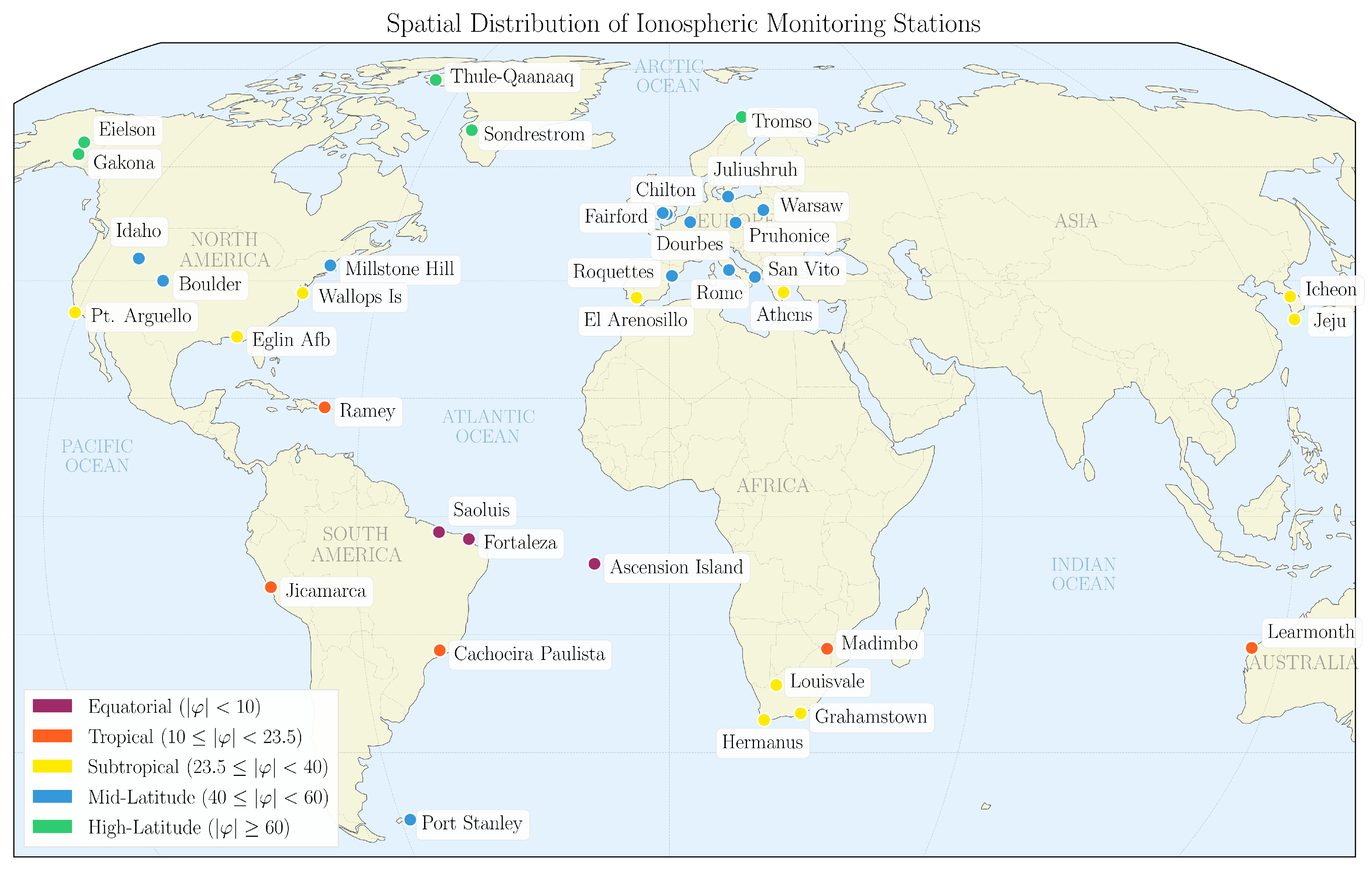
Figure 2.
Temporal availability of ionospheric data (blue shaded regions) and seismic events (red circles, scaled by magnitude) across a small sample of our stations.
Figure 2.
Temporal availability of ionospheric data (blue shaded regions) and seismic events (red circles, scaled by magnitude) across a small sample of our stations.
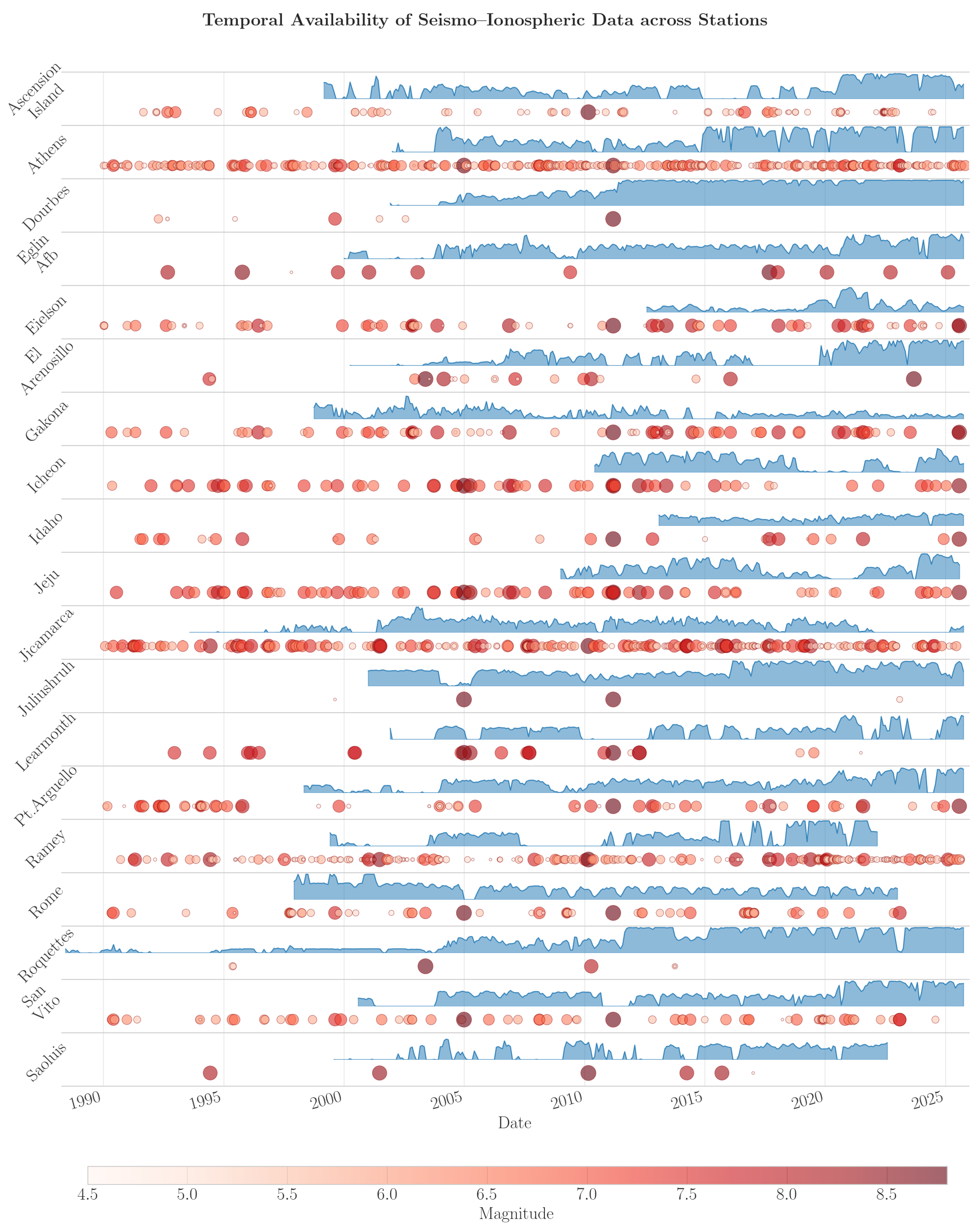
Figure 3.
Correlation of space weather features with earthquake periodicity and ionospheric parameters. Each point represents a space weather feature, with color indicating the ratio of ionospheric to seismic correlation. The optimal region (upper-left, highlighted) contains features with strong ionospheric coupling but weak earthquake periodicity correlation, minimizing temporal leakage.
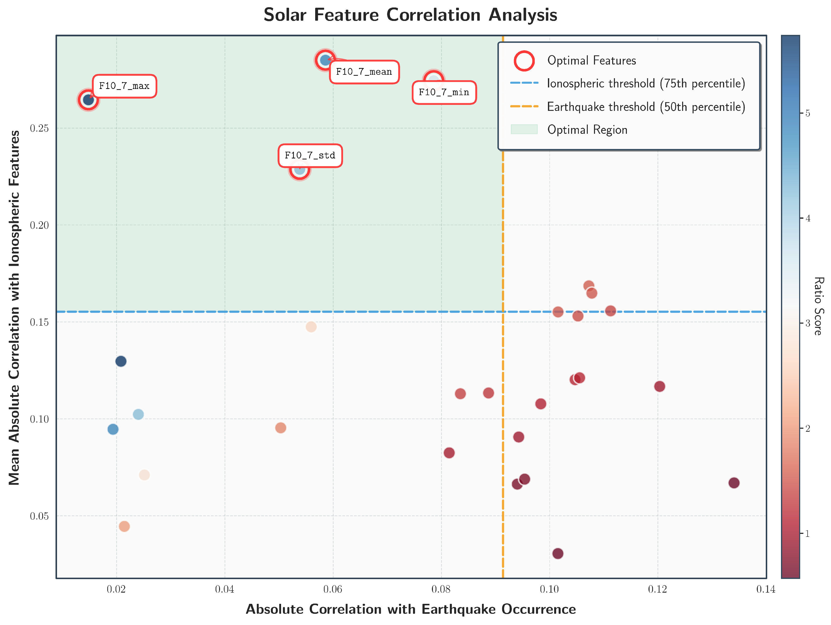
Figure 4.
Global temporal distribution of earthquakes showing pronounced year-to-year variability.
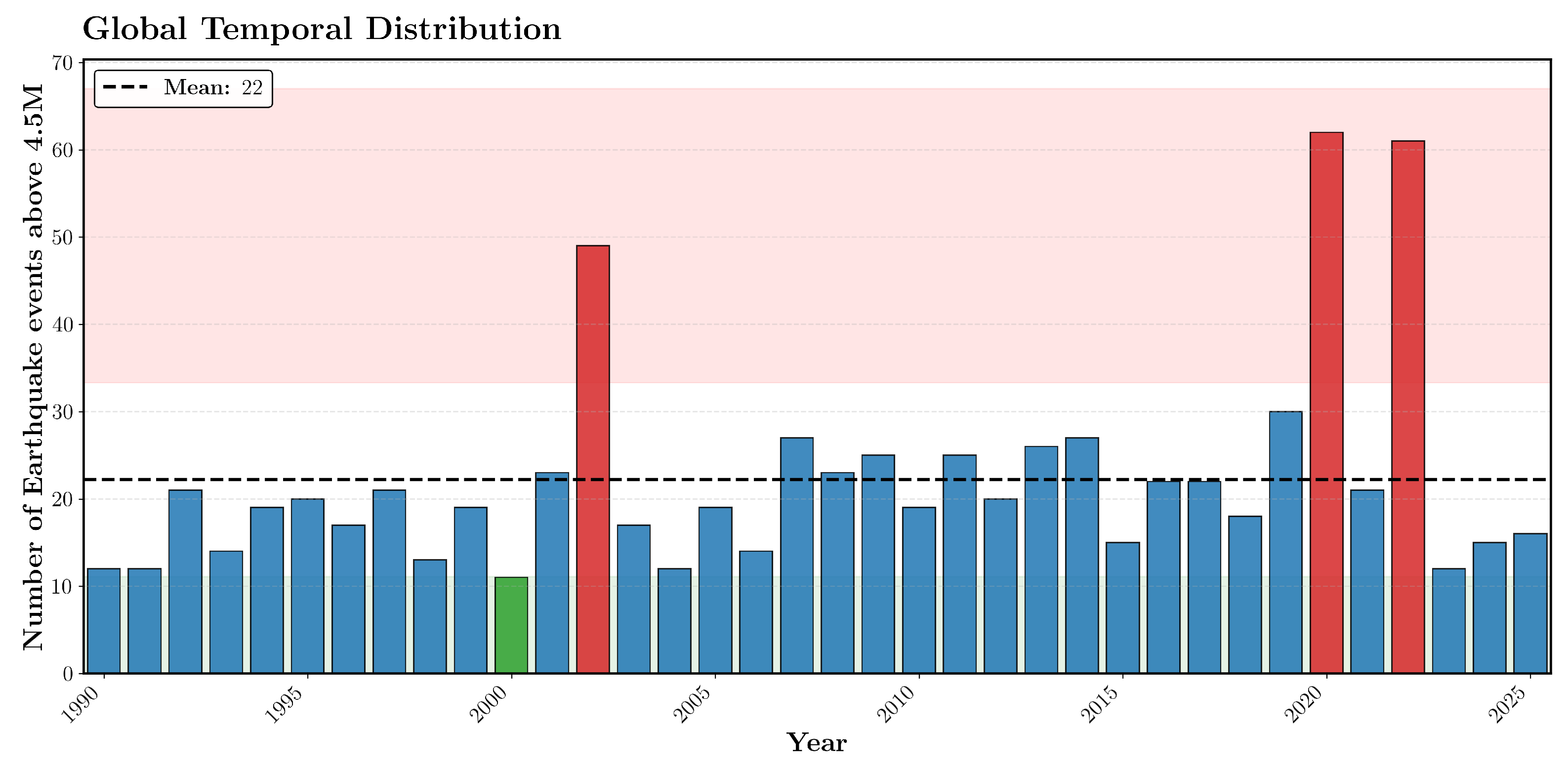
Figure 5.
Regional-temporal heatmap of earthquake frequency across some stations and years. Darker regions indicate elevated seismic activity, demonstrating heterogeneous temporal patterns across locations.
Figure 5.
Regional-temporal heatmap of earthquake frequency across some stations and years. Darker regions indicate elevated seismic activity, demonstrating heterogeneous temporal patterns across locations.
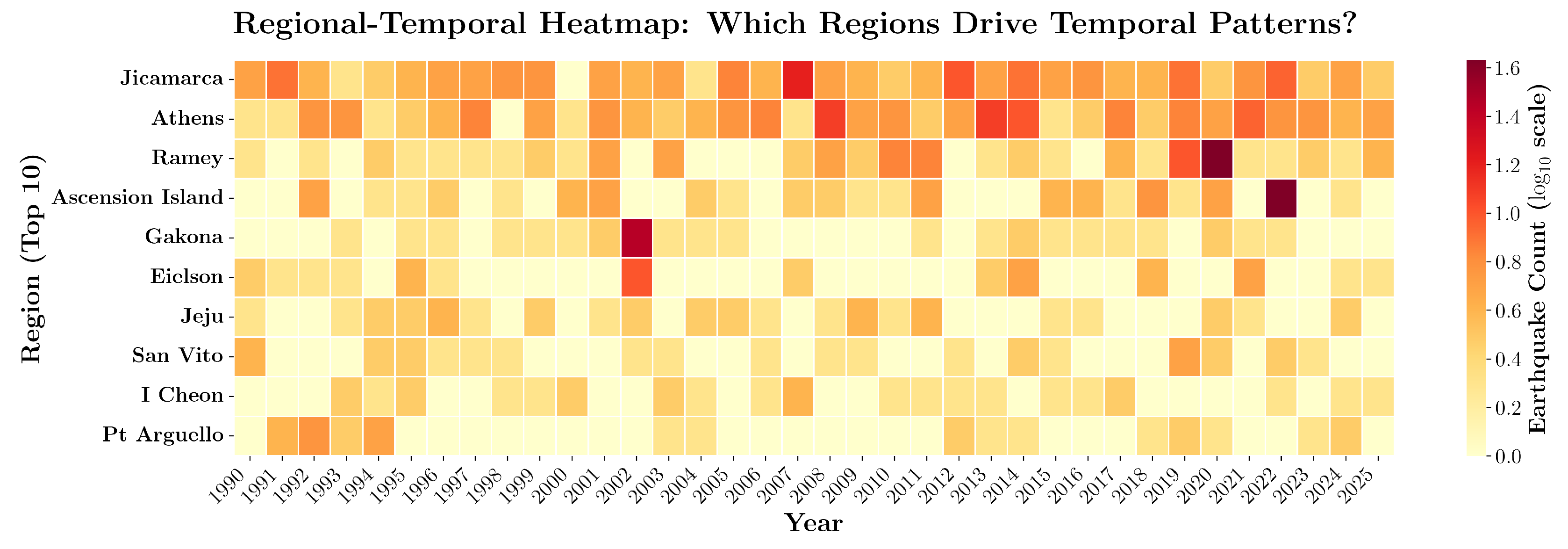
Figure 6.
Results from the Dobrovolsky relaxation factor systematic analysis.
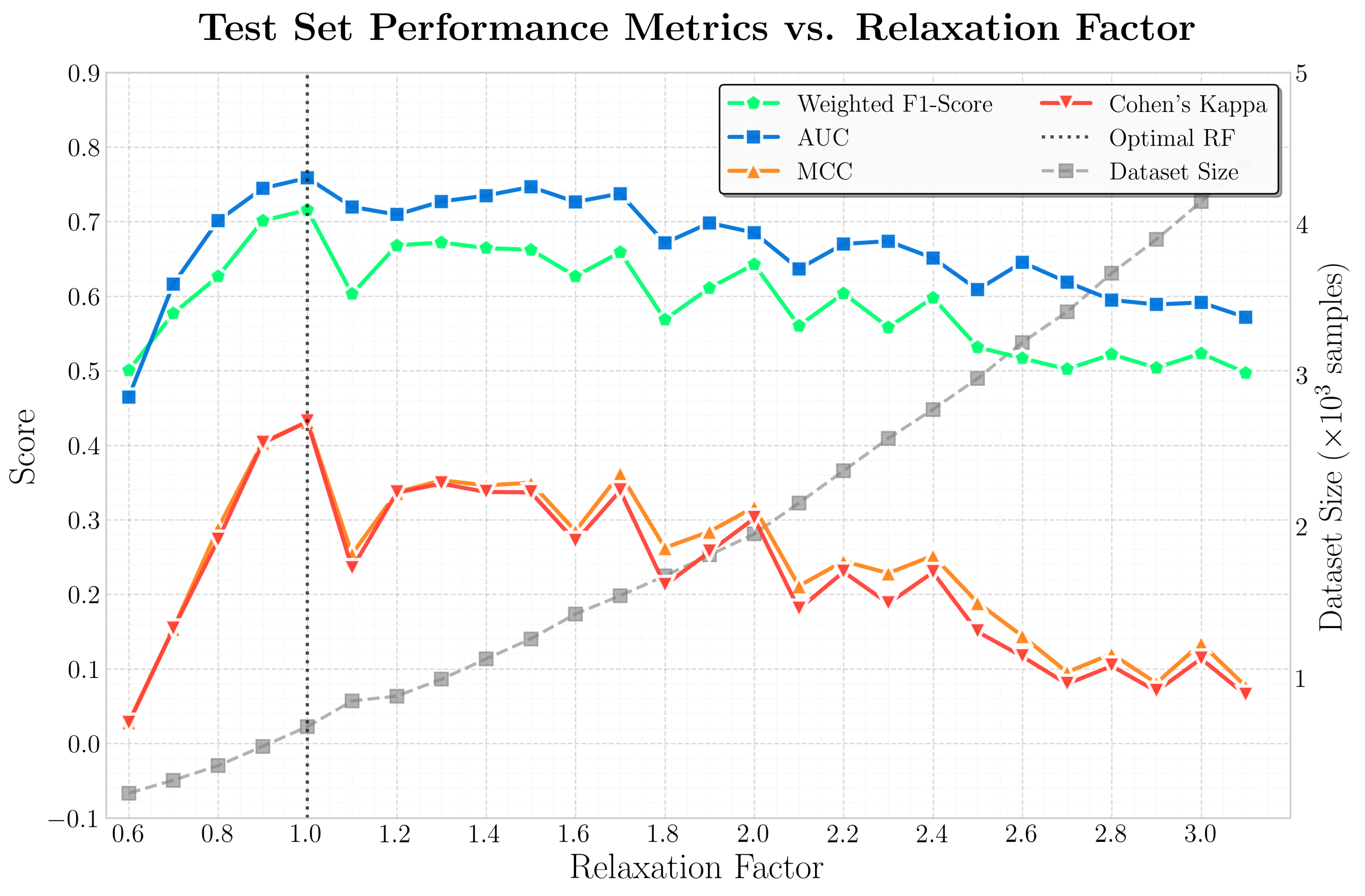
Figure 7.
Gradient Boosting confusion matrix on temporal test set.
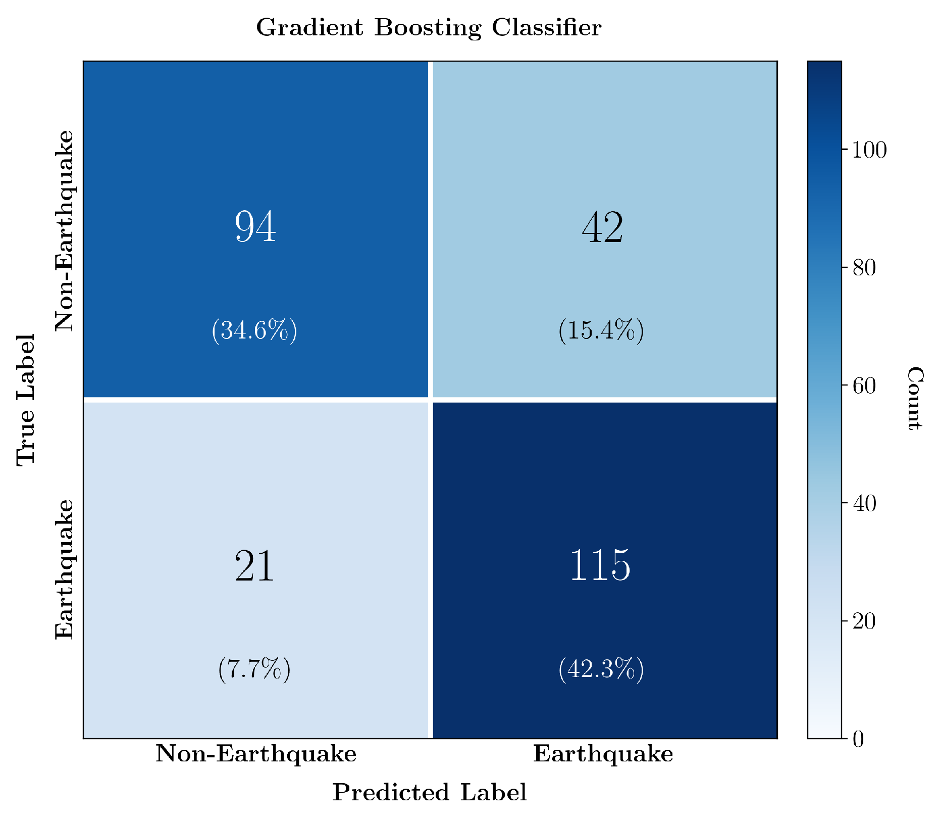
Figure 8.
Taylor diagram showing regression model performance. The reference point represents perfect predictions. Models closer to the reference with higher correlation and lower normalized standard deviation demonstrate superior magnitude prediction capability.
Figure 8.
Taylor diagram showing regression model performance. The reference point represents perfect predictions. Models closer to the reference with higher correlation and lower normalized standard deviation demonstrate superior magnitude prediction capability.
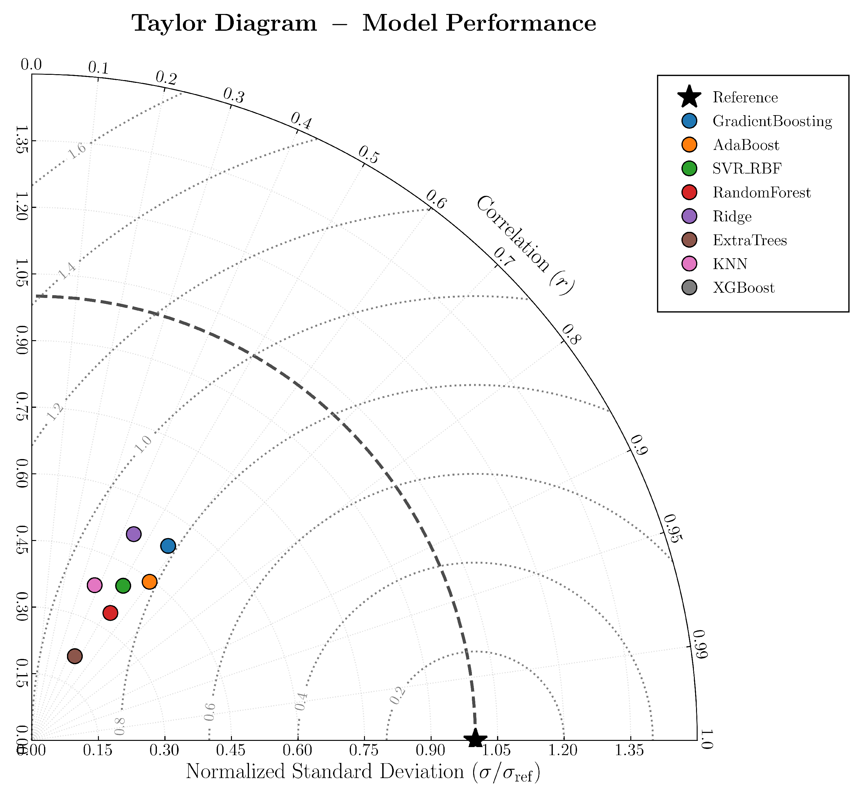
Figure 9.
Normalized feature importance comparison across selected tree-based models.
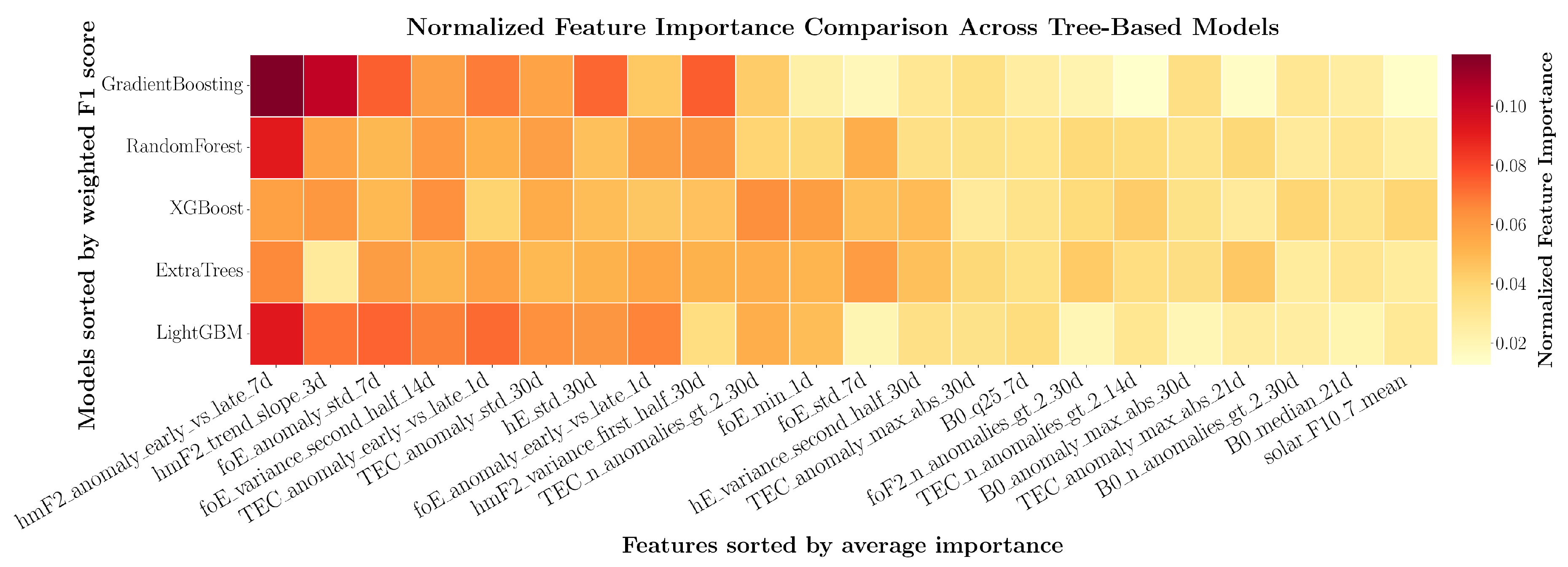

Table 1.
Classification performance on temporal test set.
| Model | F1-W | MCC | AUC | Bal-Acc |
|---|---|---|---|---|
| Gradient Boosting | 0.767 | 0.543 | 0.828 | 0.768 |
| Random Forest | 0.755 | 0.524 | 0.815 | 0.757 |
| XGBoost | 0.753 | 0.511 | 0.831 | 0.754 |
| Extra Trees | 0.753 | 0.511 | 0.816 | 0.754 |
| AdaBoost | 0.724 | 0.469 | 0.815 | 0.728 |
| Hist Gradient Boosting | 0.727 | 0.458 | 0.809 | 0.728 |
| LightGBM | 0.716 | 0.457 | 0.804 | 0.721 |
| KNN | 0.712 | 0.429 | 0.774 | 0.713 |
| SVM (RBF) | 0.704 | 0.416 | 0.768 | 0.706 |
| Logistic Regression | 0.698 | 0.398 | 0.749 | 0.699 |
| Naive Bayes | 0.682 | 0.373 | 0.741 | 0.684 |
| Elastic Net | 0.691 | 0.384 | 0.735 | 0.691 |
| Neural Network | 0.666 | 0.345 | 0.771 | 0.669 |
| Deep Neural Network | 0.658 | 0.316 | 0.724 | 0.658 |
Disclaimer/Publisher’s Note: The statements, opinions and data contained in all publications are solely those of the individual author(s) and contributor(s) and not of MDPI and/or the editor(s). MDPI and/or the editor(s) disclaim responsibility for any injury to people or property resulting from any ideas, methods, instructions or products referred to in the content. |
© 2025 by the authors. Licensee MDPI, Basel, Switzerland. This article is an open access article distributed under the terms and conditions of the Creative Commons Attribution (CC BY) license (http://creativecommons.org/licenses/by/4.0/).
Copyright: This open access article is published under a Creative Commons CC BY 4.0 license, which permit the free download, distribution, and reuse, provided that the author and preprint are cited in any reuse.


