
Submitted:
16 May 2025
Posted:
16 May 2025
You are already at the latest version
Abstract
The Third Pole region, particularly the Hindu-Kush-Himalaya (HKH), is highly prone to lightning, causing thousands of fatalities annually. Skillful prediction and timely communication are essential for mitigating lightning-related losses in such observationally data-sparse regions. Therefore, this study evaluates kilometer-scale ICON-CLM-simulated atmospheric variables using six machine learning (ML) models to detect lightning activity over the Third Pole. Results from the ensemble boosting ML models show that ICON-CLM simulated variables such as relative humidity (RH), vorticity (vor), 2m temperature (t_2m), surface pressure (sfc_pres), among a total of 25 variables, allow better spatial and temporal prediction of lightning activities, achieving a Probability of Detection (POD) of ∼ 0.65. The Lightning Potential Index (LPI) and the product of convective available potential energy (CAPE) and precipitation (prec_con), referred to as CP (i.e., CP = CAPE × precipitation), serve as key physics aware predictors, maintaining a high Probability of Detection (POD) of ∼ 0.62 with a 1–2 hour lead time. Sensitivity analyses additionally using climatological lightning data showed that while ML models maintain comparable accuracy and POD, climatology primarily supports broad spatial patterns rather than fine-scale prediction improvements. As LPI and CP reflect cloud microphysics and atmospheric stability, their inclusion, along with spatiotemporal averaging and climatology, offers slightly lower, yet comparable, predictive skill to that achieved by aggregating 25 atmospheric predictors. Finally, model evaluation using the Technique for Order of Preference by Similarity to Ideal Solution (TOPSIS) highlights XGBoost as the best-performing diagnostic classification (yes/no lightning) model across all six ML tested configurations.
Keywords:
ISS-LIS
; Lightning
; Third Pole
; Himalayas
; Machine Learning
1. Introduction
The Indian subcontinent experiences a lightning maximum during the pre-monsoon season, with a secondary peak from late August to October [1,2]. Daggar, Pakistan (34.45°N, 72.35°E), located in the western Himalayas, is Asia’s top-ranked lightning hotspot [2]. The Tropical Rainfall Measuring Mission (TRMM) - Lightning Imaging Sensor (LIS) observations reveal that the Himalayan region is one of the world’s most lightning-prone zones [3]. The rough terrain, distinct topography, and varied atmospheric circulation cause significant spatiotemporal variability in lightning flash density over the Himalayan region [3].
Lightning is an electrostatic discharge that produces an illuminated flash of light in the sky, often accompanied by thunder. Broadly accepted, the non-inductive charging mechanism explains that lightning occurs within thunderstorm clouds due to charge separation between ice particles, as collisions of ice crystals and graupel in the presence of supercooled liquid water facilitate the transfer of electrical charge [4,5]. Charged particles separate due to gravity and convection, forming oppositely charged regions within the cloud, leading to lightning when the electrical potential reaches a sufficiently high threshold [5]. Thunderstorm clouds, typically 5–10 km wide and at least 4 km deep, can generate multiple lightning flashes per second for 30–60 minutes [6]. Lightning poses a significant hazard in the Nepal Himalayas due to strong monsoonal activity and the region’s complex orography, with 2,501 reported events between 1971 and 2019 resulting in 1,927 fatalities and over 20,000 people affected [7]. The intense heating from positive lightning discharges, reaching temperatures up to 30,000 K, underscores their destructive potential [8].
In recent decades, researchers have significantly advanced lightning forecasting; shifting from traditional methods based on observational data to NWP models, and more recently, accelerating progress through ML techniques [9,10]. Price and Rind (1992) developed a lightning parameterization, known as PR92, for the WRF model based on cloud top height and vertically integrated ice water path and CAPE, resulting in better capture of spatial lightning patterns [11]. A previous study predicted lightning by post-processing NWP ECMWF ensemble output for the European Eastern Alps region by proposing a statistical lightning prediction model [12]. Furthermore, researchers widely acknowledge the critical role of data assimilation in NWP models for extending forecast horizons and improving accuracy. Mueller and Barleben (2024) reviewed the experimental ICON-RUC (rapid update cycle) model and emphasized that combining it with the nowcasting method JuliaTSnow significantly improves short-term (0–6 hour) forecasting skill. This enhancement, evidenced by increased Critical Success Index (CSI) scores (> 0.5), stems from the model’s rapid update cycles and higher spatial resolution [14]. The author later showed that for RUC, the CSI score remains above the critical threshold (0.5) for forecasts within 3 hours of data assimilation, but drops below this value for longer lead times [14]. The decline underscores limitations in the model’s physics, which struggle to accurately predict thunderstorms due to the inherent unpredictability described by chaos theory. Studies also show that deep learning methods attain enhanced thunderstorm prediction (POD = 0.60 ±0.02) through purely data-driven approaches, surpassing current NWP capabilities for short-term forecasts [14,15].
A previous study reported improved lightning prediction during the monsoon season using a random forest (RF) regression model (R-squared score = 0.81), with predictors derived from LIS satellite observations, ERA5 reanalysis, and MODIS data [16]. Further, Geng et al. (2021) developed LightNet+, a data-driven lightning forecast model using ConvLSTM, which effectively integrates WRF simulation data, past lightning data, and Automatic Weather Station (AWS) data [10]. The results indicate that LightNet+ outperforms the three established schemes PR92, F1, and F2 achieving higher POD by 22%, 36%, and 26%, respectively. This improvement reflects enhanced forecasting skill with the integration of additional data sources. In summary, significant advances in lightning prediction and modelling have emerged in last few years, from simple ML models to enhancing observational data with ML and post-processing NWP models using statistical and ML techniques. Recent studies have trained ML models for lightning prediction using observation data [16,21]. However, in data-sparse regions such as the Himalayan-Tibetan complex, where high-elevation terrain and northwestern areas face critical gaps in ground observations and satellite-derived climate records exhibit persistent uncertainties [17]. We train our ML models using the ICON-CLM NWP model, an approach that remains largely unexplored. In this framework, ML based lightning prediction with lead time relies entirely on the forecasting skill of the NWP model, rather than on extensive observational data. Therefore, NWP models coupled with ML approach can prove beneficial in advancing climate studies.
Building on our previous research by Singh and Ahrens (2023) [6], our aim is to enhance the accuracy and realism of the ICON-CLM dynamical model by post-processing the dynamic parameters governing lightning occurrence using simple ML models. We also examine the dependency of various variables in predicting lightning occurrence and identify the most robust and best-performing ML model for this highly dynamic and uncertain phenomenon. This paper is structured as follows: Section 2 details the data and methodology, including the datasets and models used. Section 3 discusses our experimental results, key findings, and potential limitations. Finally, Section 4 offers a concise conclusion summarizing our study.
2. Data and Methodology
2.1. Lightning Observation
In this study, we have used the International Space Station (ISS) based Lightning Imaging Sensor (LIS) observations from October 2019 to September 2020. The LIS is a satellite-based instrument that detects the global distribution and variability of total lightning, including cloud-to-cloud (CC), intra-cloud (IC), and cloud-to-ground (CG). LIS detects storm scale resolution (∼ 4 km) at millisecond timing with a narrow band filter (777 nanometers) in conjunction with a high-speed charge-coupled device (CCD) detection array[18]. A limitation of ISS-LIS is its 90-minute revisit time over a given region, which restricts the temporal frequency of observations [18]. A flash comprises groups of lightning events that occur within 330 ms and 5.5 km, where each group represents simultaneous events in adjacent pixels. The flash child count quantifies the number of constituent groups per flash [19].
The flow chart in Figure 1 outlines the selection process for spatiotemporal lightning events and extraction of input data for ML models in this study. Firstly we filtered the ISS-LIS swaths to focus exclusively on the Third Pole region (25°N - 40°N, 70°E - 115°E).We subsequently segregated 36,975 verified lightning flash counts recorded over domain region between October 2019 and September 2020. To improve robustness and reduce bias, we added an equal number of false instances (no lightning detected) from ISS-LIS measurements, selecting them randomly while maintaining proportionality to the monthly density of true events. Using this ISS-LIS data, we identified the time and location of lightning activity, and at these points, we extracted the corresponding 25 ICON-CLM model variables for training the ML models. We then divided the dataset into 80% for training and 20% for testing, conducting further analysis and metric calculations on the test set. Furthermore, TRMM lightning climatology data was used to supplement the observed lightning events.
2.2. Numerical Model Setup
The Icosahedral Nonhydrostatic Weather and Climate Model in Climate Limited Area Mode (ICON-CLM), version 2.6.4, simulated the Third Pole region from October 2019 to September 2020. The simulations were conducted at a high resolution with a horizontal grid spacing of 3.3 km and 60 vertical levels extending up to 10 hPa, covering the domain 22.5–42.5°N and 67.5–117.5°E [6,20]. However, our study focuses on the subdomain 25–40°N and 70–115°E for the ML model’s training, testing, and further analysis. ICON-CLM simulation uses ECMWF’s fifth-generation atmospheric reanalysis (ERA5) as initial and boundary conditions. The model simulated 25 variables on an hourly temporal scale used in the ML models represent key physical processes associated with lightning, including atmospheric instability (4 variables), cloud properties (2), moisture and precipitation (3), and column-integrated water (2), adapted from a previous study [21] (see Table 1). Our study further augments the set with variables related to surface and radiation fluxes (5), vorticity (3), temperature (3), lightning potential index (LPI), surface elevation (z), and precipitation. Together, they form a physically meaningful and comprehensive predictor set for lightning activity.
The CAPE variable quantifies the thermodynamic energy available for convective updrafts, serving as a primary indicator of atmospheric instability essential for thunderstorm and lightning development. As discussed in Section 1, the lightning parameterization PR92, which remains widely used, including in the WRF model, relies on CAPE to estimate lightning distribution [11]. In addition, Romps et al. (2018) demonstrated that CP serves as an effective proxy for lightning, accurately capturing flash rate density over land [25]. Tippett et al. (2019) further applied the CP proxy to predict daily cloud-to-ground flash counts across CONUS (2003–2016), reporting strong regional correlations between CAPE and lightning activity [26]. While CP captures essential aspects of lightning generation, other factors, such as atmospheric moisture and wind shear also play a critical role. To account for wind shear and vertical dynamics, we incorporate the LPI, which integrates vertical velocity information within convective clouds. LPI reflects the strength of updrafts and the microphysical processes that drive charge separation, both crucial for lightning generation [27]. Multiple studies have validated the predictive utility of LPI in various regions [6,13,26,27]. Building on these insights, we adopt a physically informed feature selection strategy that prioritizes interpretability and computational efficiency. In this context, CP and LPI emerge as key predictors, aligning with the findings of Singh and Ahrens (2023) [6], and form the basis of our physics-aware modeling approach.
2.3. Machine Learning Models
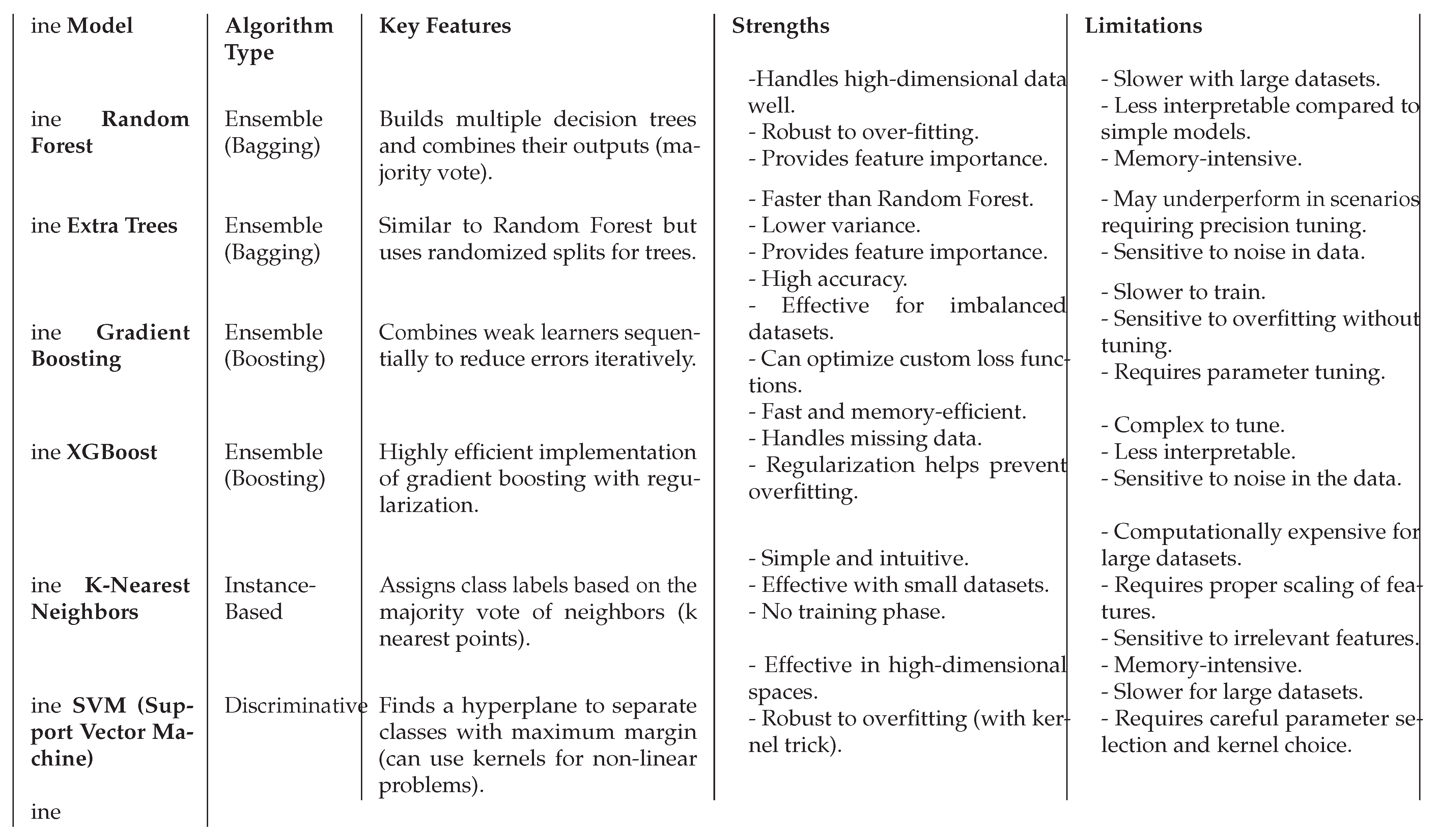
In the present study, the following ML models are used: Extra trees (ET), gradient boost (GB), K-nearest neighbors (KNN), RF, support vector machines (SVM) and extreme gradient boost (XGBoost). Our supervised learning approach employs these six models specifically selected for their distinct strengths in handling tabular lightning data. Tree-based ensemble methods (RF, ET, GB, XGBoost) are well-suited for handling noise and capturing complex relationships, while SVM effectively delineates decision boundaries. KNN, on the other hand, adapts well to localized patterns, making it particularly useful for region-specific variations. The selected ML models, optimized for structured tabular data, span from interpretable algorithms such as KNN and SVM to more complex ensemble methods like RF and XGBoost. This range allows for a balanced trade-off between interpretability and predictive performance. A detailed comparison of their strengths and limitations is provided in Appendix Table A1.
We omitted hyperparameter tuning to maintain computational efficiency and interoperability, and instead prioritized key predictor identification, as outlined in Table 1. Despite this omission, the models performed robustly, aligning with Tetko et al. (2024), who noted that hyperparameter optimization can sometimes lead to overfitting when relying on the same statistical measures [22]. To ensure a fair comparison, the six structurally distinct models (RF, ET, GB, XGBoost, KNN, SVM) using default hyperparameters allow us to isolate the impact of model architecture on performance while maintaining reproducibility and developing a transparent, physics-aware framework.
2.4. Experimental Setup
We evaluated the predictive capacity of 25 atmospheric variables for lightning using three experimental setups: direct grid point data (S1-GP) and spatial averages computed over 60 km (S1-60) and 90 km (S1-90) radii centered on each grid point - collectively termed setup S1 (Table 1). Setups S2 and S3 follow the same structure as S1, differing only in the selected input features. Additionally, an extended experiment, S3t, evaluates the effect of temporal averaging, using two approaches: one with 1-hour averages within a 60 km spatial radius (S3t-60-1h), and another with 2-hour averages within a 90 km radius (S3t-90-2h). Notably, both S3 and S3t incorporate climatology data to enrich the analysis. These setups are designed to account for spatial and temporal uncertainties, acknowledging that lightning may occur with slight spatial or temporal offsets from predicted locations.
3. Results and Discussion
The Third Pole region, encompassing the Himalayan mountains and the Tibetan Plateau (70°–110°E, 25°–40°N; Figure 2), emerges as a prominent lightning hotspot in Asia, as indicated by both our analysis and long-term observations from the TRMM satellite [23] Figure 2a presents the TRMM lightning climatology over the Third Pole region, derived from LIS and optical transient detector observations spanning 1998 to 2013. TRMM suggests that the western Himalayan region has the highest lightning incidents, followed by the Brahmaputra Valley (26°N, 90°E) and the central/eastern Himalayan ranges, as reported in previous studies [6,23]. Figure 2b shows the WWLLN daily gridded lightning data from October 2019 to September 2020, which displays spatial patterns broadly consistent with the TRMM climatology. WWLLN observation shows lower lightning events over the western Himalayan region compared to the Brahmaputra valley (Figure 2b). In addition, the WWLLN record shows more lightning incidents over the eastern Tibetan Plateau than in the TRMM climatology. The detection discrepancies between TRMM and WWLLN likely arise due to differences in the observational capabilities of the respective sensors, while TRMM detects all types of lightning flashes including CC, IG and CG, WWLLN primarily detects CG flashes [18,24]. We use lightning flash density data from ISS-LIS, to assess lightning activity across the study region. TRMM climatology and ISS-LIS lightning observations were gridded to 0.5°×0.5°- spatial resolution to match the native grid of the WWLLN dataset. The spatial distribution of ISS-LIS lightning activity during the study period closely resembles the TRMM climatology, indicating consistency in the observed patterns (Figure 2c), thereby reinforcing the reliability of ISS-LIS as a valid ground truth dataset for training ML models.
We evaluate the performance of the ML models using several standard classification metrics (see Table 2). In this context, a True Positive (TP) refers to correctly predicting lightning when it actually occurs. A False Positive (FP), or false alarm, occurs when the model predicts lightning that is not observed in the ISS-LIS data. A False Negative (FN), or missed event, occurs when the model fails to predict lightning that is observed. A True Negative (TN) refers to correctly predicting no lightning when no lightning is observed. All metric values range from 0 (worst) to 1 (best), except for the False Alarm Rate (FAR), where lower values indicate better performance; thus, we report 1–FAR for consistency. ROC-AUC stands for Receiver Operating Characteristic – Area Under the Curve.
Based on the lightning patterns observed in Figure 2 c, we used six ML models to reconstruct and evaluate the spatial lightning activity, aiming to assess their predictive skill across the study domain. Figure 3 presents a heat map depicting the performance of S1 experiments across multiple metrics. The rows represent different models and experiments, such as ET, GB, KNN, RF, SVM and XGBoost. Each model was evaluated using point data and aggregated data at spatial scales of 60 km and 90 km. The columns correspond to different performance metrics, including Accuracy, CSI, POD, Precision, ROC-AUC, 1-FAR.
The XGBoost model consistently achieves top performance across most evaluation metrics, particularly for spatially averaged datasets (60 km and 90 km). For instance, XGBoost-S1-90 attains highest accuracy (0.63), POD (0.66), and ROC AUC (0.68), highlighting its ability to effectively utilize aggregated data. Spatial averaging enhances overall model performance, with KNN and RF models showing notable improvements in accuracy and CSI at S1-60 and S1-90 compared to the grid-point configuration (S1-GP); suggesting that aggregation aids in capturing broader spatial patterns and mitigating noise. While GB and XGBoost perform robustly across all metrics. ET demonstrates stable performance across scales but shows less sensitivity to spatial averaging. In contrast, SVM consistently underperforms, particularly in accuracy and CSI, indicating limited capability in detecting TP events.
A comparative analysis of multiple metrics alone makes it difficult to definitively identify the optimal model and discern the underlying influence of specific predictors. Thus, it is equally important to examine which of the 25 predictors most strongly influence the ML predictions. Examining feature importance therefore supports interpretability and enables potential feature reduction. Figure 4 illustrates the relative contribution of each of the 25 input variables (predictors) to the predictive outputs of all six models in the experimental setup S1-90. The feature importance of other experiments (S1-GP, S1-60), are presented in the supplementary results in Figure S2. In the given Figure 4, the horizontal axis represents the variables (features) used to train the model; see the list of variables in Table 1. RF and ET, belonging to the ensemble learning family of models, exhibit nearly parallel trends that closely align with fluctuations, including spikes and lows with respective features. ET and RF models exhibit relatively uniform feature importance distributions, which can make them less effective at identifying the most influential features. Due to their ensemble nature, averaging across many weak learners they tend to assign importance in a moderate and somewhat diffuse manner, limiting their ability to distinctly highlight the most relevant features. The randomly assignments of weights to 25 variables show that all features receive nearly equal importance (see Figure 4). Such uniform distribution of feature importance suggests that the model lacks reliability in distinguishing key predictors. Unlike ET/RF, GB produces sharper importance peaks for key features like T_850 and precipitation, likely reflecting its iterative residual-learning process that progressively emphasizes the most influential predictors [28]. Although in the real physical world, almost 50% of the variable features exhibit strong inter-correlation and interdependence that should negatively influence the learning process of ML models. The inconsistent emphasis on features such as z, thb_s and RH highlights the ambiguity in model interpretation, underscoring the need for physics-informed feature selection to ensure meaningful and domain-relevant insights. Therefore, as discussed in Section 2.2, we test the predictability of the ML models using the key predictors CAPE and LPI in experiment S2.
The S2 experiment simulation yielded results comparable to the 25-feature experiment S1. While accuracy and other metrics showed slight variations, models like XGBoost and GB maintained a POD of 0.6. Figure 5 presents the S2 experiment heat map, evaluating the isolated importance of CP and LPI. Despite relying solely on these two predictors, the ML models achieve performance comparable to that of the S1 experiment, reaffirming their dominant dynamic influence on the prediction task. A sensitivity experiment incorporating TRMM climatology data (S3) reveals no measurable improvement in model prediction skill (Supplementary Figure S1). Although the integration of multi-source data was expected to enhance model learning [11], the findings indicate minimal additional benefit from climatological inputs in the context of this specific prediction objective.
Lightning is a localized phenomenon wherein thunder clouds can traverse significant distances before striking the ground. Consequently, models may correctly detect lightning events yet misidentify their precise location or timing. Therefore averaging predictions over 1- and 2-hour intervals can enhance detection consistency and reduce localization errors. The S3t experiment (Figure 6) incorporates time-averaged CP and LPI variables, building upon the previous experimental framework. This configuration demonstrates superior performance across all models compared to S2 and S3, while maintaining high predictive accuracy with only a marginal reduction (0.02-0.04) relative to S1. The results suggest that temporal averaging of these key dynamical variables effectively preserves predictive skill while enhancing model stability. Meanwhile, the margin-based optimization model (SVM) shows a rise in the POD, which is crucial. The ensemble boosting models (XGboost, GB) still maintain similar accuracy to Sets 1, 2, and 3. It is important to note the remarkable similarity ( especially XGBoost, POD ∼0.6) in S1 and S3t. This indicates that the six ML models are optimized to generate consistent predictions for the 25 variables, as well as the two time-averaged diagnosed variables (CP and LPI), when combined with the climatological data. Spatial averaging (grid → 60 km → 90 km) systematically improves skill scores (accuracy, precision, POD, ROC-AUC) individually in S 1,2,3 and 3t confirming mesoscale integration as critical for lightning predictability. In S1, the XGBoost model shows a 3–4% improvement in accuracy and ROC-AUC from S1-GP to S1-90 (Figure 3), a trend similarly observed in S2 and S3. Additionally, in S2 and S3, RF and ET also exhibit a 3% accuracy increase over the same spatial range in comparison to S1. Thus time and space averaging consistently improves model performance over grid-point values.
To identify the best-performing ML model within each experiment set and across all experiments, we employ a multi-criteria decision analysis method, TOPSIS (see supplementary results for Equation S1) [29]. A model with a high TOPSIS score is closer to the ideal solution (value ≈ 1), indicating strong performance across multiple metrics. It has a smaller Euclidean distance from the ideal solution and a larger distance from the anti-ideal solution ((value ∼ 0). Figure 7 illustrates the top 5 ranking models across individual sets and combined for all experiments. For S1, XGBoost achieves the highest TOPSIS score for S1-90. In contrast, KNN emerges as the best model for S3t with a TOPSIS score of 0.82, ranking second best in S1. RF shows consistency with the two-variable experiments (S2 and S3). Additionally, an overall evaluation across all experiments confirms XGBoost as the highest-ranking model, with TOPSIS scores of 0.99 and 0.94 for S1-90 and S1-60, respectively, demonstrating consistent performance across different spatiotemporal settings (S1 – S3t).
The spatial prediction performance of our top-performing XGBoost model (Figure 7) is presented across the Third Pole region (Figure 8). Figure 8a displays the observed lightning event density from ISS-LIS, while Figure 8b shows regions with no lightning during ISS-LIS overpasses. XGBoost reproduces lightning hotspots in the western Himalayan region (Figure 8c) but under-represents the Brahmaputra Valley region. At the same time, Figure 8d shows the reverse, where no lightning (clear sky) events are predicted well over the Brahmaputra Valley region. This regional performance contrast reflects fundamental differences in convective regimes: the western Himalayas are characterized by deep convection generating intense but infrequent lightning, while the Brahmaputra Valley features shallow convection producing frequent but weaker events [6,23]. These distinct regimes may require tuning of both NWP and ML approaches, enhancing parameterizations in mountainous terrain. Figure 8e shows locations where the model falsely predicted lightning but did not occur in observation (FP), and Figure 8f shows the missed events (FN) that the model failed to predict when lightning was observed in reality. Although FP and FN occur with lower intensity, it suggests the model struggles with predictor sensitivity or misclassified convective signals.
Our study employs ISS-LIS satellite observations exclusively as ground truth for lightning identification, with model training restricted to one year of ICON-CLM simulation data. Unlike previous studies that employed neural networks and reanalysis data, our approach relies on simpler ML models. Despite these constraints, our model’s performance metrics—POD, FAR, CSI, and ROC-AUC—remain comparable to or slightly lower than those reported in past research [30,31,32]. Vahid Yousefnia et al. (2024) applied ICON data with a feedforward neural network for pixel-wise thunderstorm prediction up to 11 hours ahead, achieving skill metrics (CSI, POD) comparable to our results [21]. The present study similarly leverages ICON-CLM data but adopts a computationally efficient XGBoost model tailored for tabular inputs, identifying key predictors for lightning forecasts while maintaining robust performance.
4. Conclusions
This study demonstrates that machine learning models can effectively predict lightning activity in the Third Pole region by leveraging dynamically relevant atmospheric variables. Through the systematic evaluation of six ML models (ET, RF, XGBoost, GB, SVM, KNN) across four experimental sets, we identify LPI and CP as the most critical predictors, achieving comparable accuracy to models using 25 predictors while significantly reducing computational costs. Our results show that applying spatiotemporal averaging—particularly at 60 km (POD = 0.60) and 90 km (POD = 0.62) scale, consistently enhances model performance. Among the models evaluated, XGBoost emerges as the top-performing model, with TOPSIS scores of 0.94 (S1-60) and 0.99 (S1-90). Spatial evaluation shows the XGBoost model successfully identify lightning hotspots aligned with mountainous topography while correctly classifying stable regions, though some false alarms are encountered at some point. fig01,fig02,fig03 show that when all 25 predictors are used, the feature significance of CP and LPI are minimal, likely overshadowed by other features. However, when CP and LPI are used exclusively in a physics-based approach, the model achieves a POD of ∼ 0.60. The study framework demonstrates that physics-based NWP variables serve as effective predictors and enable efficient lightning prediction. The “LIS-ISS NO” category shown in Figure 8b likely includes instances where lightning occurred shortly before or after the satellite overpass, resulting in missed detections. Consequently, some false positives identified by the model may in fact correspond to actual lightning events that were not captured by the ISS-LIS instrument due to its temporal limitations. This introduces a degree of bias in the ML model training, potentially inflating false-positive rates (Figure 8e). Incorporating continuous ground-based lightning observations into the training process could mitigate this issue and improve model performance. Future work should expand training data period and use hybrid models while incorporating additional physical parameters to improve skill across complex topography.
Author Contributions
Conceptualization, H.J. and P.S.; methodology, H.J.; software, H.J.; validation, H.J., P.S.; formal analysis, H.J.; investigation, H.J.; resources, H.J., B.A., and J.S.; data curation, H.J., P.S.; writing—original draft preparation, H.J.; writing—review and editing, H.J., P.S., B.A., and J.S.; visualization, H.J.; supervision, P.S.; project administration, B.A., J.S.; funding acquisition, B.A., J.S. All authors have read and agreed to the published version of the manuscript.
Funding
This research was funded by the Deutsche Forschungsgemeinschaft (DFG, German Research Foundation)—TRR 301—Project-ID 428312742.
Institutional Review Board Statement
Not applicable.
Informed Consent Statement
Not applicable.
Data Availability Statement
The data presented in this study are available in the article and the supplementary material.
1. Simulated LPI data are also available https://zenodo.org/records/10053518 (accessed on 29 December 2024).
2. WWLLN Global Lightning Climatology https://zenodo.org/records/6007052
3. TRMM https://ghrc.nsstc.nasa.gov/lightning/data/data_lis_vhr-climatology.html lightning climatology
4. Data used in this study in tabulated format https://doi.org/10.5281/zenodo.15173916.
Acknowledgments
This work was Funded by the Deutsche Forschungsgemeinschaft (DFG, German Research Foundation)—TRR 301—Project-ID 428312742.
Conflicts of Interest
The authors declare no conflicts of interest.
Abbreviations
The following abbreviations are used in this manuscript:
| ISS-LIS | International Space Station - Lightning Imagining Sensors |
| WWLLN | World Wide Lightning Location Network |
| LPI | Lightning Potential Index |
| CP | CAPE times Precipitation |
| RH_850,500,300 | relative humidity at (850, 500, 300) hPa |
| vor_850,500,300 | vorticity at (850, 500, 300) hPa |
| clcm and clch | medium and high cloud cover |
| cin_ml | convective inhibition of mean surface layer parcel |
| lhfl_s and shfl_s | surface latent and sensible heat flux |
| qhfl_s | surface moisture flux |
| sob_s and thb_s | shortwave and longwave net flux at surface |
| tqc and tqi | total column integrated cloud water and ice |
Appendix A

Table A1.
Detailed Overview of ML Models.
References
- Lal, D. M., & Pawar, S. D. (2009). Relationship between rainfall and lightning over central Indian region in monsoon and premonsoon seasons. Atmospheric Research, 92(4), 402-410.
- Albrecht, R. I. , Goodman, S. J., Buechler, D. E., Blakeslee, R. J., & Christian, H. J. (2016). Where are the lightning hotspots on Earth?. Bulletin of the American Meteorological Society, 97(11), 2051-2068.
- Damase, N. P. , Banik, T., Paul, B., Saha, K., Sharma, S., De, B. K., & Guha, A. (2021). Comparative study of lightning climatology and the role of meteorological parameters over the Himalayan region. Journal of Atmospheric and Solar-Terrestrial Physics, 219, 105527.
- Saunders, C. P. R., Bax-Norman, H., Emersic, C., Avila, E. E., & Castellano, N. E. (2006). Laboratory studies of the effect of cloud conditions on graupel/crystal charge transfer in thunderstorm electrification. Quarterly Journal of the Royal Meteorological Society: A journal of the atmospheric sciences, applied meteorology and physical oceanography, 132(621), 2653-2673.
- Mostajabi, A., Finney, D. L., Rubinstein, M., & Rachidi, F. (2019). Nowcasting lightning occurrence from commonly available meteorological parameters using machine learning techniques. Npj Climate and Atmospheric Science, 2(1), 41.
- Singh, P., & Ahrens, B. (2023). Modeling Lightning Activity in the Third Pole Region: Performance of a km-Scale ICON-CLM Simulation. Atmosphere, 14(11), 1655.
- Adhikari, B. R. (2021). Lightning fatalities and injuries in Nepal. Weather, climate, and society, 13(3), 449-458.
- Adhikari, P. B. (2022). People Deaths and Injuries Caused by Lightning in Himalayan Region, Nepal. International Journal of Geophysics, 2022(1), 3630982.
- Bishop, C. M. , & Nasrabadi, N. M. (2006). Pattern recognition and machine learning (Vol. 4, No. 4, p. 738). New York: springer.
- Geng, Y. A. , Li, Q., Lin, T., Yao, W., Xu, L., Zheng, D.,... & Zhang, Y. (2021). A deep learning framework for lightning forecasting with multi-source spatiotemporal data. Quarterly Journal of the Royal Meteorological Society, 147(741), 4048-4062.
- Price, C., & Rind, D. (1992). A simple lightning parameterization for calculating global lightning distributions. Journal of Geophysical Research: Atmospheres, 97(D9), 9919-9933.
- Simon, T. , Mayr, G. J., Umlauf, N., & Zeileis, A. (2019). NWP-based lightning prediction using flexible count data regression. Advances in Statistical Climatology, Meteorology and Oceanography, 5(1), 1-16.
- Uhlířová, I. B., Popová, J., & Sokol, Z. (2022). Lightning Potential Index and its spatial and temporal characteristics in COSMO NWP model. Atmospheric Research, 268, 106025.
- Müller, R. , & Barleben, A. (2024). Data-Driven Prediction of Severe Convection at Deutscher Wetterdienst (DWD): A Brief Overview of Recent Developments. Atmosphere, 15(4), 499.
- Brodehl, S. , Müller, R., Schömer, E., Spichtinger, P., & Wand, M. (2022). End-to-End Prediction of Lightning Events from Geostationary Satellite Images. Remote Sensing, 14(15), 3760.
- Chatterjee, C., Mandal, J., & Das, S. (2023). A machine learning approach for prediction of seasonal lightning density in different lightning regions of India. International Journal of Climatology, 43(6), 2862-2878.
- Rameshan, A. , Singh, P., & Ahrens, B. (2025). Cross-Examination of Reanalysis Datasets on Elevation-Dependent Climate Change in the Third Pole Region. Atmosphere, 16(3), 327.
- Lang, Timothy & National Center for Atmospheric Research Staff (Eds). Last modified 2023-09-04 "The Climate Data Guide: Lightning data from the TRMM and ISS Lightning Image Sounder (LIS): Towards a global lightning Climate Data Record.” Retrieved from https://climatedataguide.ucar.edu/climate-data/lightning-data-trmm-and-iss-lightning-image-sounder-lis-towards-global-lightning on 2025-02-26.
- Mach, D. M. , Christian, H. J., Blakeslee, R. J., Boccippio, D. J., Goodman, S. J., & Boeck, W. L. (2007). Performance assessment of the optical transient detector and lightning imaging sensor. Journal of Geophysical Research: Atmospheres, 112(D9).
- Singh, P. , & Ahrens, B. (2023). Lightning Potential Index Using ICON Simulation at the km-scale over the Third Pole Region: ISS-LIS events and ICON-CLM simulated LPI. Zenodo. [CrossRef]
- Vahid Yousefnia, K. , Bölle, T., Zöbisch, I., & Gerz, T. (2024). A machine-learning approach to thunderstorm forecasting through post-processing of simulation data. Quarterly Journal of the Royal Meteorological Society, 150(763), 3495-3510.
- Tetko, I. V. , van Deursen, R., & Godin, G. (2024). Be aware of overfitting by hyperparameter optimization!. Journal of Cheminformatics, 16(1), 1-11.
- Cecil, D. J. , Buechler, D. E., & Blakeslee, R. J. (2014). Gridded lightning climatology from TRMM-LIS and OTD: Dataset description. Atmospheric Research, 135, 404-414.
- Rodger, C. J. , Brundell, J. B., Holzworth, R. H., & Lay, E. H. (2009, April). Growing detection efficiency of the world wide lightning location network. In AIP Conference Proceedings (Vol. 1118, No. 1, pp. 15-20). American Institute of Physics.
- Romps, D. M. , Charn, A. B., Holzworth, R. H., Lawrence, W. E., Molinari, J., & Vollaro, D. (2018). CAPE times P explains lightning over land but not the land-ocean contrast. Geophysical Research Letters, 45(22), 12-623.
- Saleh, N., Gharaylou, M., Farahani, M. M., & Alizadeh, O. (2023). Performance of lightning potential index, lightning threat index, and the product of CAPE and precipitation in the WRF model. Earth and Space Science, 10(9), e2023EA003104.
- Lynn, B. , & Yair, Y. (2010). Prediction of lightning flash density with the WRF model. *Advances in Geosciences, 23*, 11–16. [CrossRef]
- Natekin A, Knoll A. (2013). Gradient boosting machines, a tutorial. Front Neurorobot. [CrossRef] [PubMed] [PubMed Central]
- El Alaoui, M. (2021). Fuzzy TOPSIS: Logic, Approaches, and Case Studies. CRC Press. [CrossRef]
- Tippett, M. K. , & Koshak, W. J. (2018). A baseline for the predictability of US cloud-to-ground lightning. Geophysical Research Letters, 45(19), 10-719.
- Mansouri, E., Mostajabi, A., Tong, C., Rubinstein, M., & Rachidi, F. (2023). Lightning Nowcasting Using Solely Lightning Data. Atmosphere, 14(12), 1713.
- Leinonen, J. , Hamann, U., & Germann, U. (2022). Seamless lightning nowcasting with recurrent-convolutional deep learning. Artificial Intelligence for the Earth Systems, 1(4), e220043.
- Giannaros, T. M., Kotroni, V., & Lagouvardos, K. (2015). Predicting lightning activity in Greece with the Weather Research and Forecasting (WRF) model. Atmospheric Research, 156, 1-13.
- Uhlířová Babuňková, I., Popová, J., & Sokol, Z. (2022). Lightning Potential Index and its spatial and temporal characteristics in COSMO NWP model. Atmospheric Research, 268, 106025. [CrossRef]
- Yair, Y. , Lynn, B., Price, C., Kotroni, V., Lagouvardos, K., Morin, E.,... & Llasat, M. D. C. (2010). Predicting the potential for lightning activity in Mediterranean storms based on the Weather Research and Forecasting (WRF) model dynamic and microphysical fields. Journal of Geophysical Research: Atmospheres, 115(D4).
- Zängl, G. , Reinert, D., Rípodas, P., & Baldauf, M. (2015). The ICON (ICOsahedral Non-hydrostatic) modelling framework of DWD and MPI-M: Description of the non-hydrostatic dynamical core. Quarterly Journal of the Royal Meteorological Society, 141(687), 563-579.
- Pham, T. V., Steger, C., Rockel, B., Keuler, K., Kirchner, I., Mertens, M., ... & Früh, B. (2021). ICON in Climate Limited-area Mode (ICON release version 2.6. 1): a new regional climate model. Geoscientific Model Development, 14(2), 985-1005.
- Poelman, D. R. , & Schulz, W. (2020). Comparing lightning observations of the ground-based European lightning location system EUCLID and the space-based Lightning Imaging Sensor (LIS) on the International Space Station (ISS). Atmospheric Measurement Techniques, 13(6), 2965-2977.
Figure 1.
Schematic workflow of data preprocessing and filtering, including the extraction of spatially and temporally collocated features from the ICON-CLM simulation corresponding to ISS-LIS observations; used for training ML models and predictive evaluation.
Figure 1.
Schematic workflow of data preprocessing and filtering, including the extraction of spatially and temporally collocated features from the ICON-CLM simulation corresponding to ISS-LIS observations; used for training ML models and predictive evaluation.
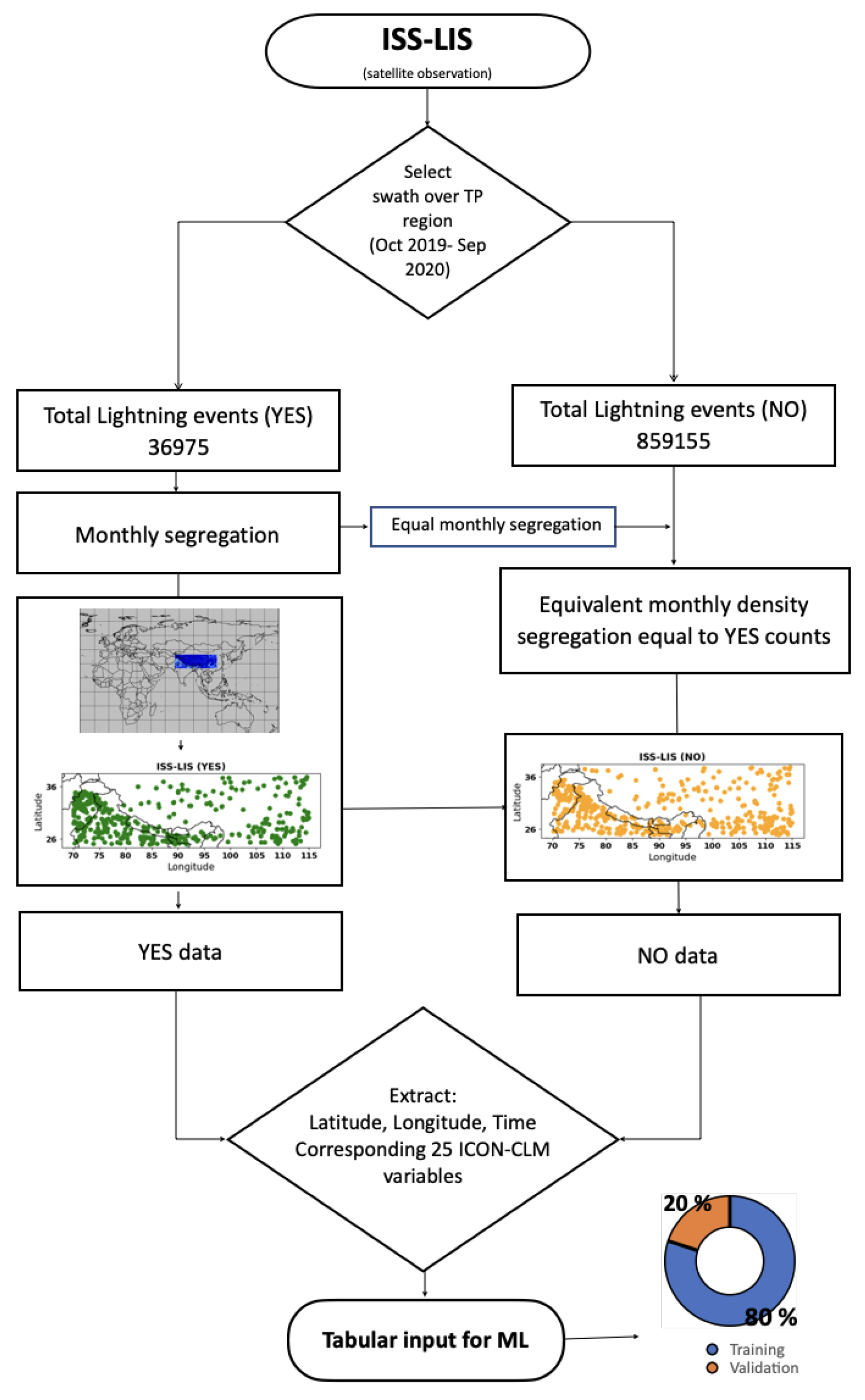
Figure 2.
(a) The lightning climatology from TRMM (1998-2013), (b) Total observed lightning events from WWLLN (October 2019 - September 2020) and (c) ISS-LIS (October 2019 - September 2020) over the Third Pole region. Grey line represents topography contour ≥ 4000m.
Figure 2.
(a) The lightning climatology from TRMM (1998-2013), (b) Total observed lightning events from WWLLN (October 2019 - September 2020) and (c) ISS-LIS (October 2019 - September 2020) over the Third Pole region. Grey line represents topography contour ≥ 4000m.
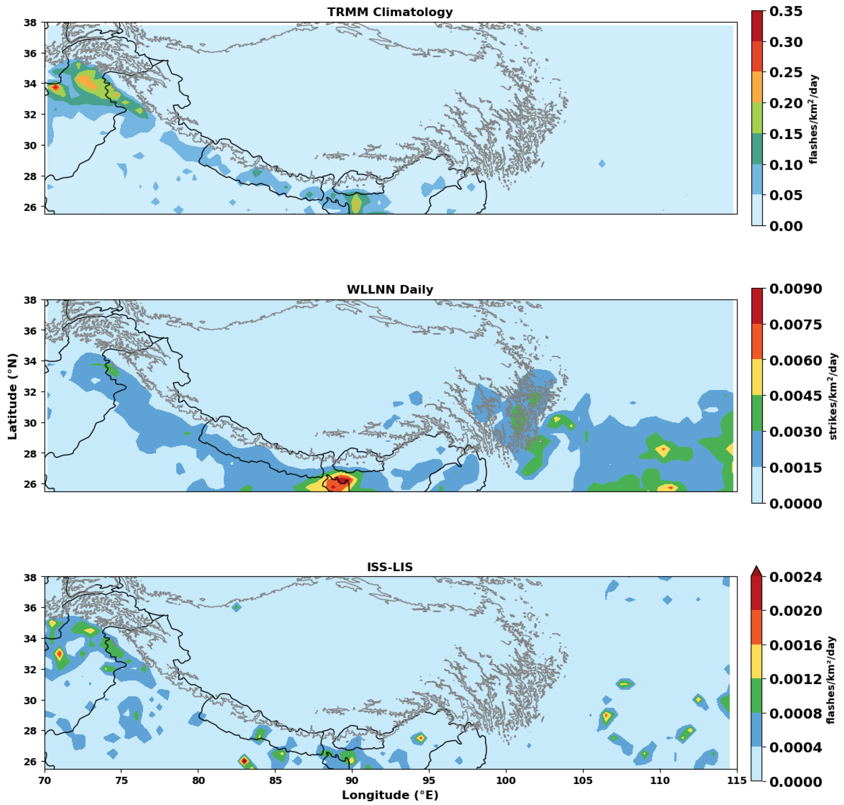
Figure 3.
Comparison of the metrics from the S1 experiments with all 6 models and 25 model predictors.
Figure 3.
Comparison of the metrics from the S1 experiments with all 6 models and 25 model predictors.
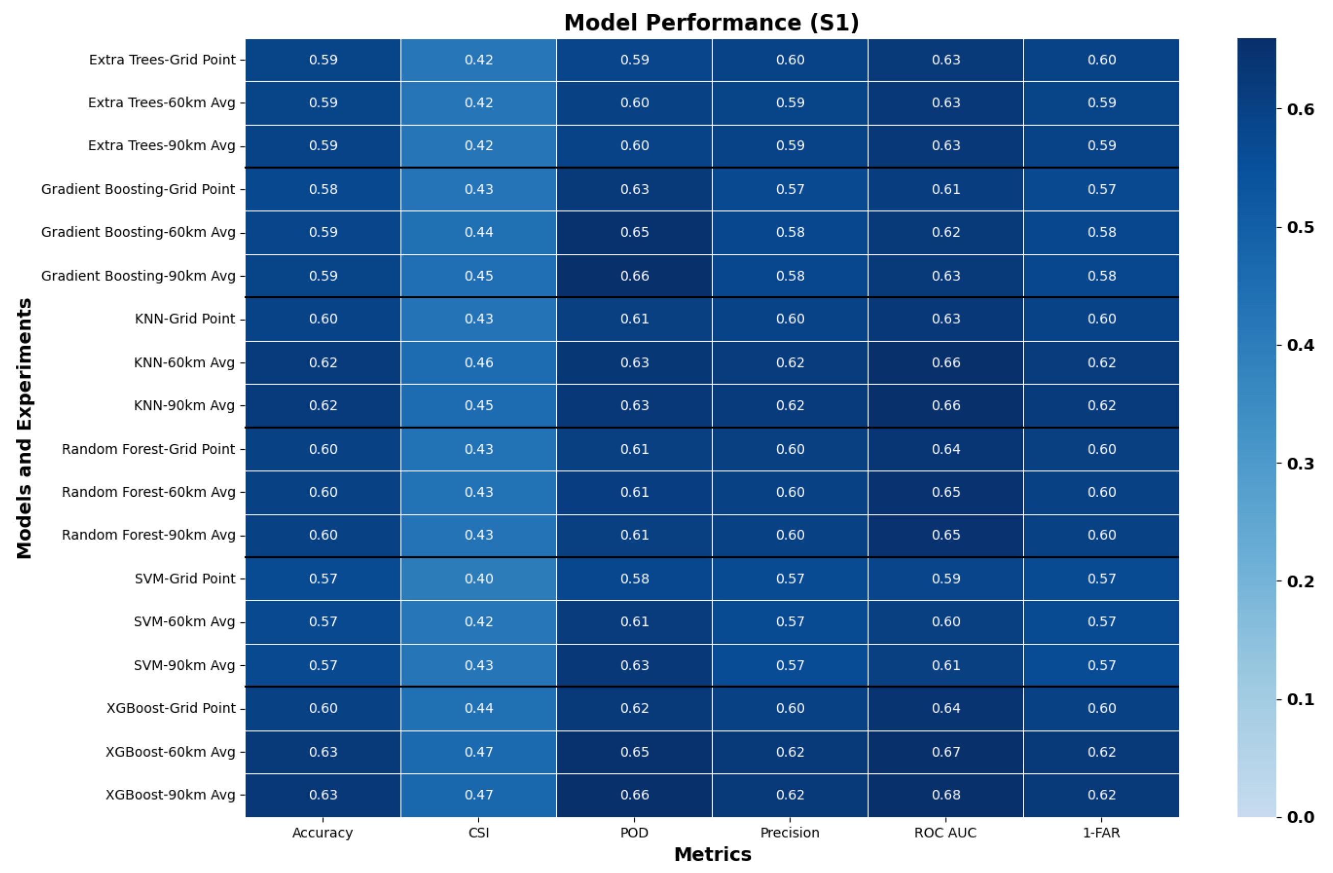
Figure 4.
Features significance for all six models at S1-90 experimental setup.
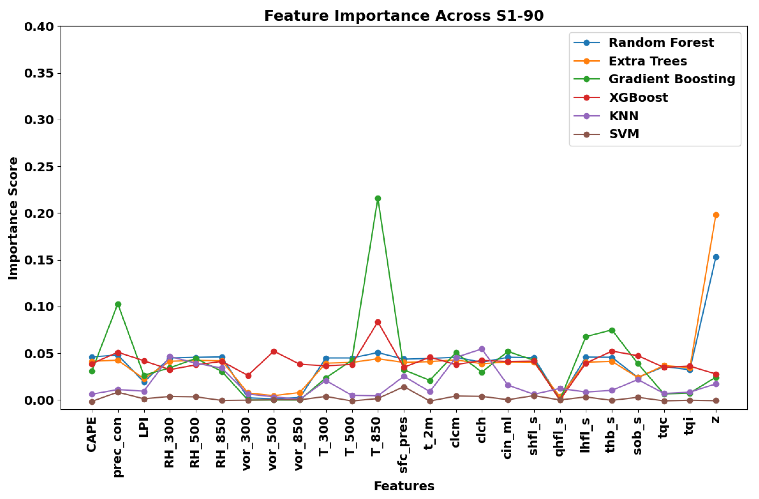
Figure 5.
Comparison of the metrics for the S2 experiment with all 6 models.
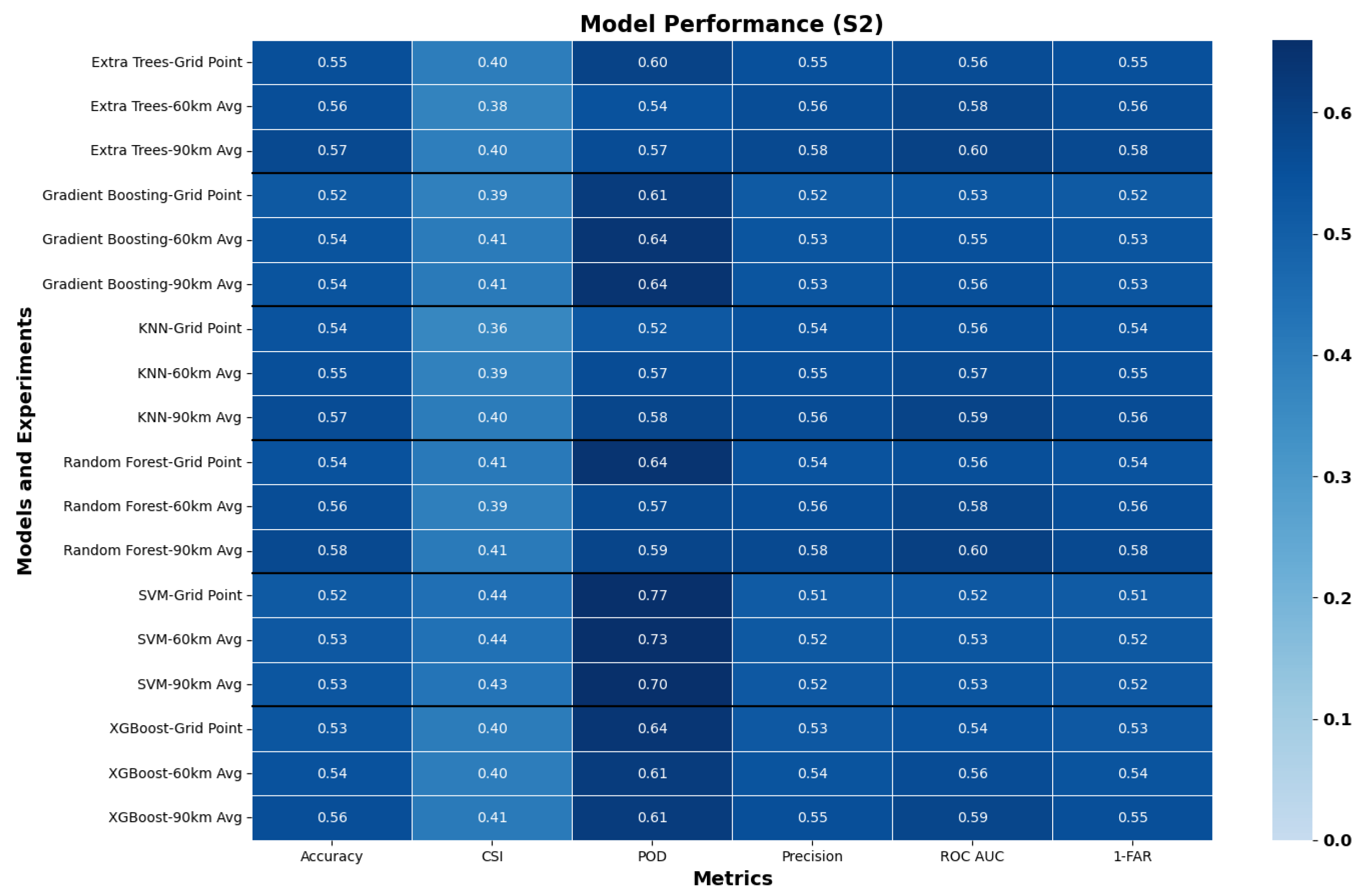
Figure 6.
Comparison of the metrics from the S3t experiments with all six models and CP, LPI and Climatology
Figure 6.
Comparison of the metrics from the S3t experiments with all six models and CP, LPI and Climatology
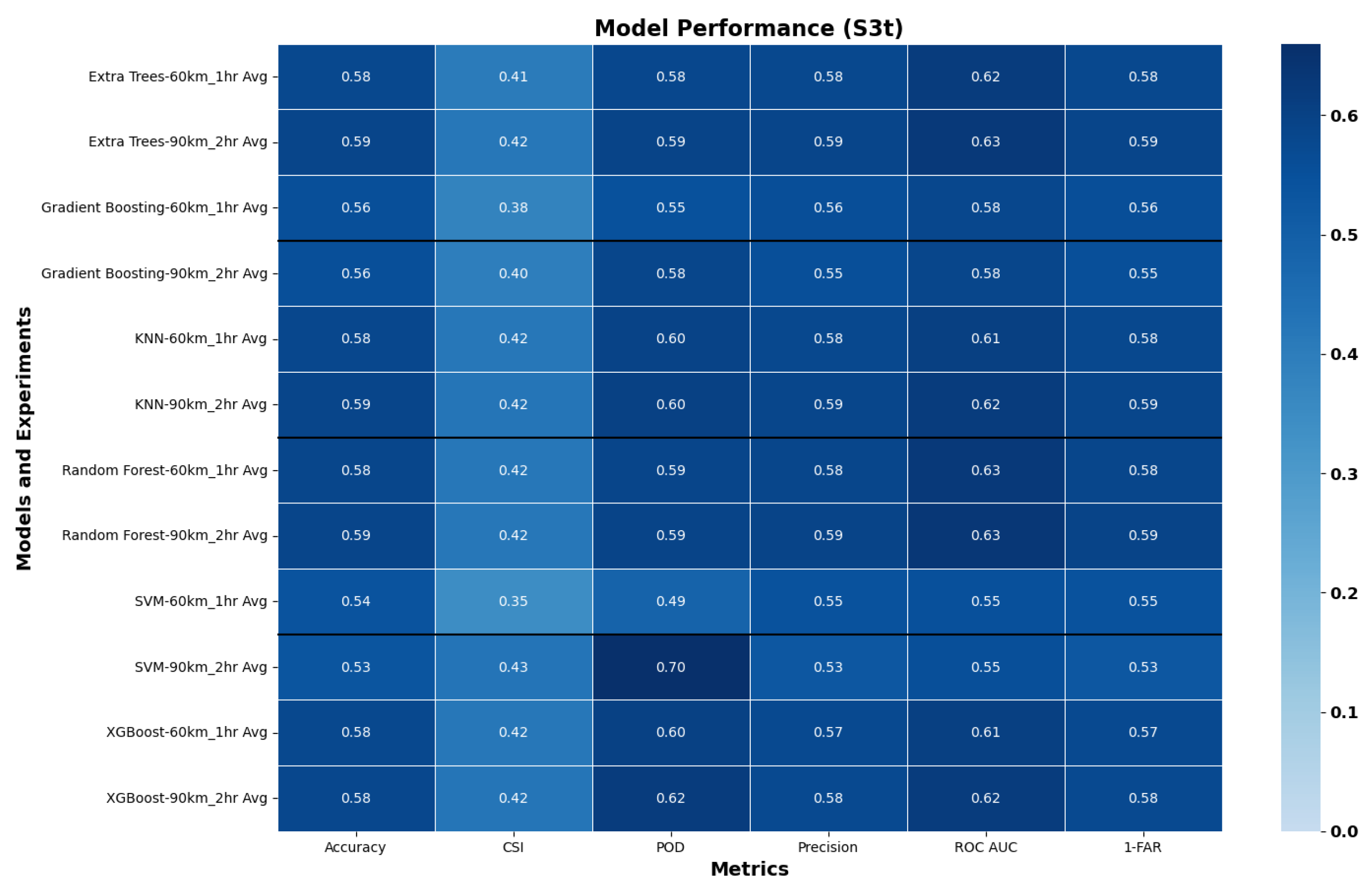
Figure 7.
TOPSIS score for the experimental set 1-3t for all experiments.
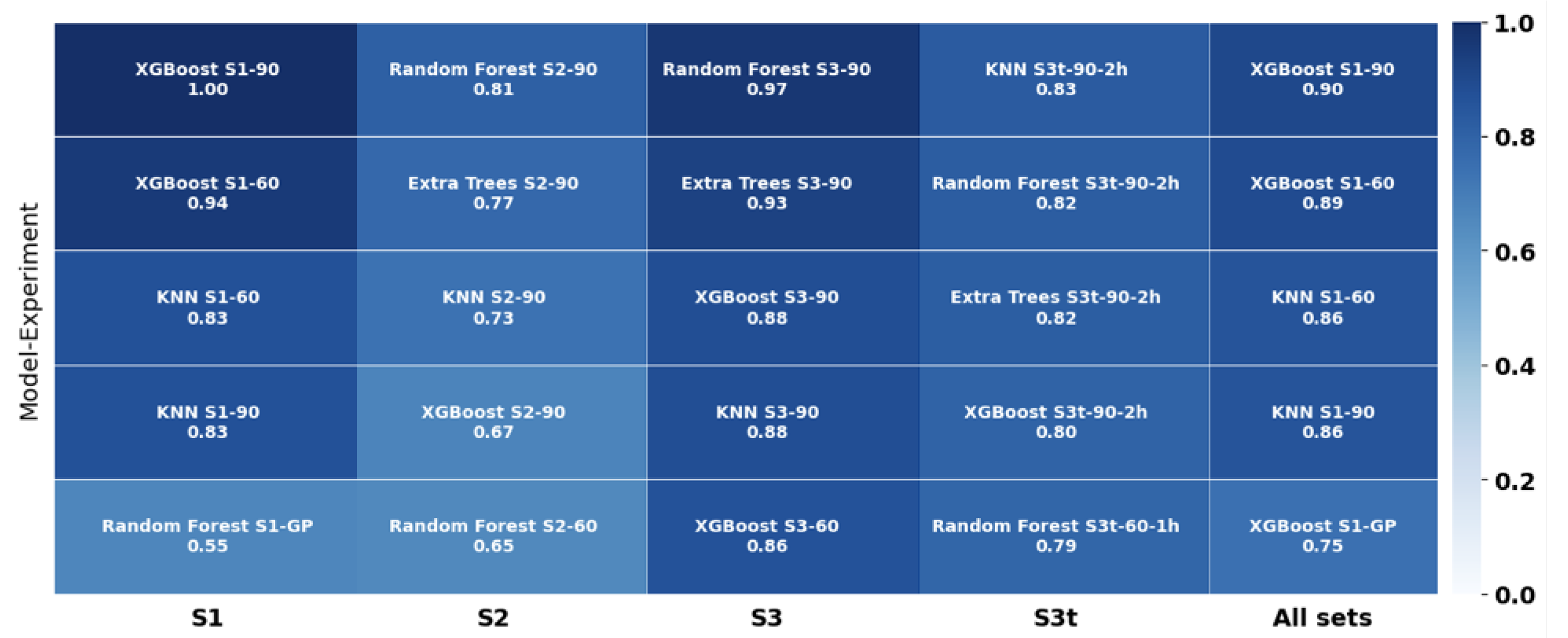
Figure 8.
Panels (a) and (b) show the spatial distribution of lightning density (flashes/km²) and no-lightning events based on ISS-LIS observations. Panels (c)–(f) illustrate the XGBoost model’s prediction outcomes over the test dataset from October 2019 to September 2020, presented in terms of confusion matrix components.
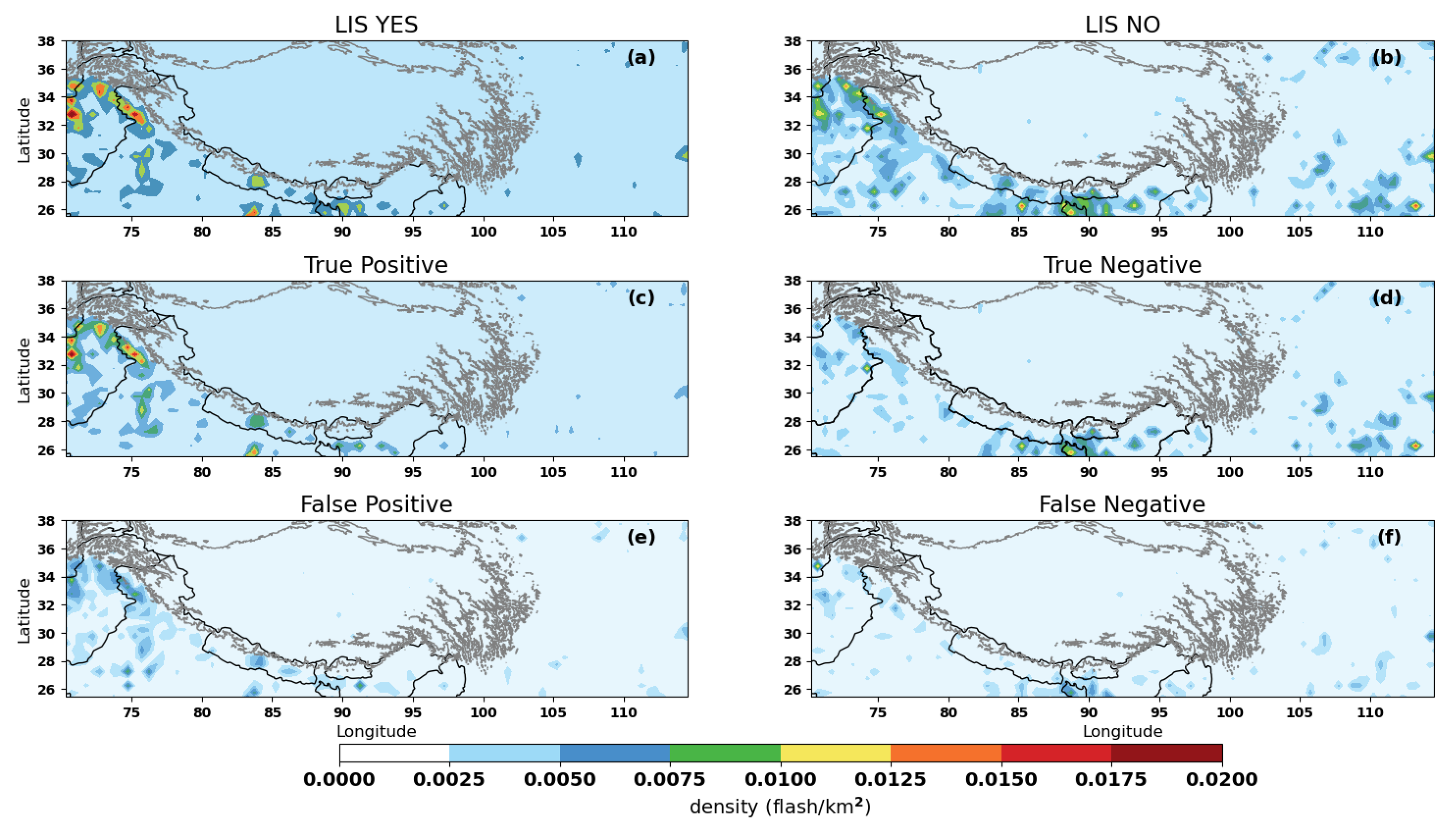
Table 1.
Summary of experiments with different spatial-temporal coverages and variable sets. (See Appendix A for abbreviations)
Table 1.
Summary of experiments with different spatial-temporal coverages and variable sets. (See Appendix A for abbreviations)
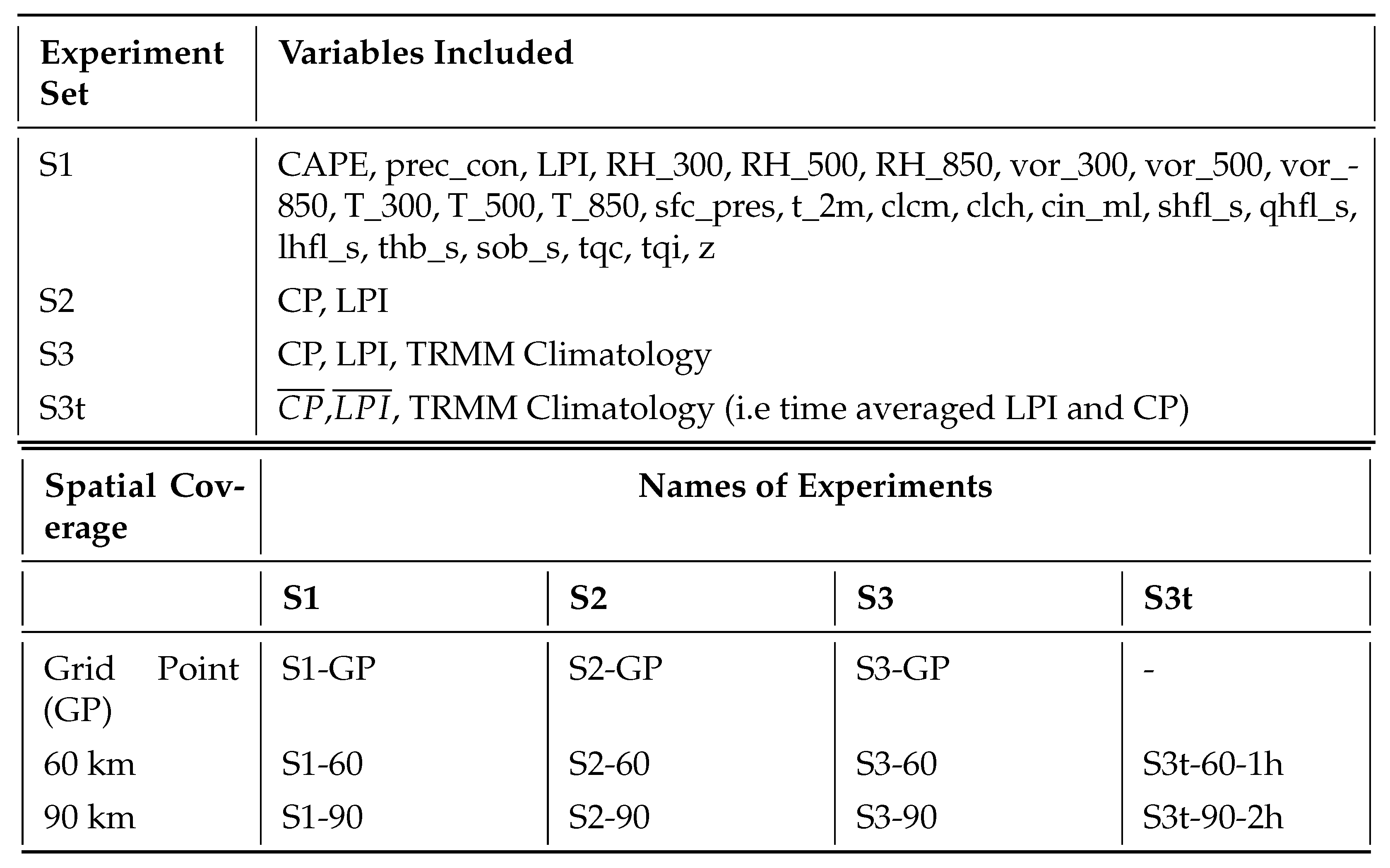
Table 2.
Summary of evaluation Metrics. Note:.
| Metric | Formula | Interpretation |
|---|---|---|
| Accuracy | Overall correctness of the model | |
| Precision | Measures how many predicted events actually happened | |
| POD(Recall) | Measures how well the model detects actual events | |
| FAR | Measures how many predicted events were false alarms | |
| CSI | Balances between false alarms and missed events | |
| ROC-AUC | Measures model’s ability to distinguish classes (lightning and no-lightning) |
Disclaimer/Publisher’s Note: The statements, opinions and data contained in all publications are solely those of the individual author(s) and contributor(s) and not of MDPI and/or the editor(s). MDPI and/or the editor(s) disclaim responsibility for any injury to people or property resulting from any ideas, methods, instructions or products referred to in the content. |
© 2025 by the authors. Licensee MDPI, Basel, Switzerland. This article is an open access article distributed under the terms and conditions of the Creative Commons Attribution (CC BY) license (http://creativecommons.org/licenses/by/4.0/).
Copyright: This open access article is published under a Creative Commons CC BY 4.0 license, which permit the free download, distribution, and reuse, provided that the author and preprint are cited in any reuse.


