Submitted:
30 April 2025
Posted:
02 May 2025
You are already at the latest version
Abstract
This study systematically investigates pre-seismic ionospheric anomalies preceding the 2023 Jishishan Ms6.2 earthquake using Total Electron Content (TEC) data derived from BDS Geostationary Orbit (GEO) satellites. Multi-scale analysis integrating Butterworth filtering and wavelet transforms decoupled TEC disturbances into three distinct frequency regimes: (1) High-frequency perturbations (0.56–3.33 mHz) manifest as localized disturbances (amplitude ≤4 TECU, range <300 km), attributed to near-field acoustic waves from crustal stress release; (2) Mid-frequency anomalies (0.28–0.56 mHz) exhibit anisotropic propagation (>1,200 km) with azimuth-dependent N-shaped waveforms, driven by acoustic-gravity waves (AGWs); (3) Low-frequency signals (0.18–0.28 mHz) display phase reversal and non-linear amplitude attenuation following a power-law relationship, indicative of stress-mediated lithosphere-atmosphere-ionosphere (LAI) coupling oscillations. A stark contrast between near-field residuals and far-field weak fluctuations highlights the dominance of large-scale atmospheric gravity waves over localized acoustic disturbances. Geometry-based velocity inversion revealed incoherent high-frequency dynamics (5–30 min) versus anisotropic mid/low-frequency TID propagation (30–90 min) at 175–270 m/s, consistent with AGW theory. Despite concurrent G1-class geomagnetic storm activity, spatial attenuation gradients and velocity anisotropy confirm seismogenic origins, providing critical evidence for earthquake precursor discrimination and advancing multi-scale coupling mechanisms in ionospheric monitoring.
Keywords:
2023 Jishishan Ms6.2 Earthquake
; BDS GEO
; TEC
; acoustic-gravity wave
; seismo-ionospheric anomaly
1. Introduction
The investigation of seismo-ionospheric anomalies has garnered significant attention as a critical precursor for short-term earthquake forecasting [1,2,3]. Since the first recorded ionospheric perturbations preceding the 1964 Alaska MW9.2 earthquake, advancements in Global Navigation Satellite System (GNSS)-derived Total Electron Content (TEC) monitoring have revolutionized the detection and characterization of ionospheric anomalies associated with seismic activity [4,5,6]. Empirical studies suggest that majority of earthquakes with magnitudes exceeding Mw6.0 exhibit complex pre-seismic TEC variations [7]. Then GPS-derived TEC monitoring has become the cornerstone for pre-earthquake ionospheric anomaly detection, with well-documented cases including: the anomalous TEC attenuation preceding the 1999 Taiwan Chi-Chi Mw7.7 earthquake [8], the multi-phase TEC fluctuations observed before the 2008 Wenchuan Mw7.9 earthquake [9], the pre-seismic ionospheric anomalies preceding the 2013 Mw7.7 Pakistan earthquake [10], the pronounced positive TEC anomalies over the epicentral and magnetic conjugate regions within two weeks preceding the 2021 Yangbi–Maduo twin earthquakes [11], and the g ionospheric TEC anomalies associated with the 2024 Mw7.5 Noto Peninsula earthquake [12]. Statistical analyses further corroborate the robust correlation between seismic events and ionospheric disturbances: Liu et al. identified that approximately 80% of TEC anomalies within five days prior to Mw≥6.0 earthquakes in Taiwan were seismogenic [13], while Le et al. demonstrated a statistically significant increase in TEC anomaly frequency preceding global Mw≥6.0 earthquakes compared to background levels [14].
However, the IPPs between space satellites and ground-based receivers exhibit spatially uneven variations due to satellite motion. Consequently, the derived TEC data do not directly represent temporal variations at a fixed ionospheric location and require mathematical interpolation or modeling for spatial homogenization, introducing inherent uncertainties [15,16]. In contrast, the GEO satellites of the BeiDou Navigation Satellite System (BDS) provide a unique advantage for long-term ionospheric TEC monitoring due to their quasi-invariant orbital configurations [17]. While geostationary orbits are perturbed by Earth’s oblateness and gravitational interactions with the Sun and Moon, onboard station-keeping mechanisms minimize positional deviations, ensuring that IPP fluctuations remain negligible relative to the ionosphere’s large spatial scale (thousands of kilometers). Thus, BDS GEO satellites can be approximated as stationary relative to Earth, enabling ground stations to continuously acquire TEC data from fixed IPPs. This capability effectively establishes a network of time-continuous, position-locked monitoring nodes, significantly enhancing the spatiotemporal resolution of ionospheric observations [18,19,20].
While statistical correlations between ionospheric anomalies and seismic events have been established, significant gaps persist in our understanding of the underlying physical mechanisms governing the genesis and evolutionary processes of seismogenic ionospheric disturbances. The lithosphere-atmosphere-ionosphere coupling (LAIC) framework has emerged as a pivotal theoretical model to explain seismo-ionospheric interactions, proposing three primary coupling pathways: chemical channeling, acoustic-gravity wave (AGW) propagation, and electrostatic field modulation [21,22,23,24,25,26]. Among these, AGW-mediated coupling has gained prominence due to its traceable vertical propagation from the lithosphere to the ionosphere [27]. Seismically excited AGWs interact with ionospheric plasma through vertical energy transfer, inducing detectable TEC oscillations. For instance, Korepanov et al. employed wavelet analysis to reveal atmospheric filtering effects on AGWs, demonstrating that high-velocity, long-wavelength acoustic-gravity wave signals can propagate through the atmosphere to become captured by the ionosphere, whereas low-velocity or short-wavelength signals tend to dissipate within the atmospheric medium [28]. Notably, such high-velocity, long-wavelength acoustic-gravity wave signals are predominantly excited by surface tectonic activities such as earthquakes, rather than originating from convective weather systems. Yang et al. further validated this pathway by observing spatiotemporal coherence between stratospheric AGWs and ionospheric TEC disturbances preceding the 2016 Kumamoto earthquake [29]. Phanikumar et al. observed synchronous AGWs in VLF electromagnetic waves and mesospheric ozone anomalies prior to the 25 April 2015 Nepal Gorkha Mw7.8 earthquake [30]. Ray et al. identified dual co-seismic TIDs during the 2024 Hualien M7.4 earthquake, with velocity bifurcation (0.78 km/s vs. 0.48 km/s) potentially linked to multi-source fault rupture dynamics, highlighting the complexity of AGW-driven coupling [31]. These findings indicate that AGW coupling with the lower ionosphere not only triggers anomalous plasma oscillations but also modulates neutral atmospheric composition perturbations. The observed phenomena distinctly illustrate the vertical propagation pathway of AGWs across the troposphere-stratosphere-mesosphere (lower ionosphere) system.
Regarding the coupling mechanism between ionospheric TEC anomalies and AGWs, the E-region dynamo current hypothesis remains the most widely accepted explanation. Based on the synchronized anomalies in VLF signals and TEC variations, it is inferred that AGWs propagating to the lower ionosphere (primarily the E-region) induce wind field perturbations [32,33,34,35]. However, the precise mechanisms governing TEC-AGW synchronization remain ambiguous. Besides, current seismo-ionospheric TEC investigations predominantly employ temporally coarse datasets (e.g., global ionospheric maps with 2-hour resolution), focusing on statistical anomaly detection over pre-seismic timescales spanning days to weeks. The lack of higher-resolution spectral decomposition of ionospheric perturbations has fundamentally hindered the definitive identification of causative frequency bands underlying these anomalies. Critically, conventional GPS-derived TEC measurements inherit systematic uncertainties from their medium earth orbit (MEO) satellites. Since continuous migration of IPPs at ∼25 km/min orbital velocity introduces spatiotemporal aliasing, the derived TEC time series intrinsically conflate temporal variations and spatial plasma gradients due to IPP trajectory evolution. Besides, the orbital motion induces the amplitude attenuation in detected AGW signatures compared to stationary observations.
In light of this, this study investigates the pre-seismic ionospheric TEC anomalies and AGW coupling phenomena associated with the 18 December 2023 Gansu Jishishan Ms6.2 earthquake, utilizing high-rate TEC data from the BDS GEO satellites within the continuously operating reference stations (CORSs) of Gansu Province in China. Then we analyzed the propagation process and spatiotemporal characteristics of ionospheric disturbances on the day of the Jishishan Earthquake from multiple perspectives, including the spatiotemporal distribution, propagation velocity, time-frequency domain, disturbance amplitude, and waveform of ionospheric perturbations. It further examined the relationship between TIDs during the earthquake preparation period and weak geomagnetic storms, aiming to provide theoretical insights for studying the coupling mechanism between the ionosphere and AGWs prior to earthquakes.
2. Materials and Methods
This chapter establishes a systematic framework for ionospheric TEC retrieval, modeling, and disturbance characterization using GNSS observations. Beginning with dual-frequency code and phase measurements, it derives slant TEC (STEC) while addressing differential code biases (DCBs) through pseudorange smoothing. A Single-Layer Model (SLM) is employed to map STEC to vertical TEC (VTEC), leveraging the quasi-static geometry of GEO satellites to isolate temporal ionospheric variations. Advanced signal processing techniques—including adaptive median filtering, Butterworth bandpass filtering, and Morlet wavelet analysis—are integrated to suppress noise, extract disturbance components (DTEC), and identify dominant spectral features.
2.1. GNSS Observations and the Geometry-Free Combination
Under idealized conditions neglecting multipath effects and measurement noise, the fundamental GNSS code and carrier-phase observation equations (in length units) can be expressed as:
where and denote the code and carrier-phase measurements from receiver to satellite at frequency , respectively; is the frequency-independent composite term, comprising the geometric range (), receiver clock-bias (), satellite clock-bias () and tropospheric delay (; is the first-order ionospheric delay at reference frequency (as adopted in this study) along the line-of-sight; denotes the ionospheric scaling factor; and represent the receiver- and satellite-specific code hardware delays, respectively; is integer ambiguity term for carrier-phase; is phase hardware delay (typically absorbed into ambiguity parameters); is the speed of light in vacuum; and is wavelength.
The cumulative nature of GNSS carrier-phase observations enables millimeter-level measurement precision (2–3 orders of magnitude higher than code), making them ideal for code smoothing to enhance usable accuracy [36,37]. This study employs dual-frequency carrier-phase smoothed code (CSC) to decouple first-order ionospheric delays and hardware bias parameters, constructing a geometry-free (GF) combination with the following observation equations:
where and epresent the inter-frequency differenced code and phase observables, respectively. and denote the receiver- and satellite-end DCBs.
To achieve cascaded noise attenuation, a recursive weighting algorithm is implemented, expressed as:
where represents the adaptive smoothing window width (typical range: 2~100), initialized with [38,39]. The algorithm implicitly assumes quasi-linear ionospheric delay variations within the smoothing window. Under severe ionospheric disturbances (e.g., scintillation), window parameters require dynamic adjustment to balance noise suppression and temporal responsiveness.
2.2. Ionospheric TEC Extraction
In electromagnetic wave propagation theory, the geometric optics approximation applies when the radio wavelength is much smaller than the characteristic spatial scale of the ionosphere. Under this assumption, the signal propagation path from satellite to receiver can be modeled by integrating the phase velocity along the trajectory [40]. The ionospheric delay effect caused by wave propagation through the ionized medium is quantified as:
where is the electron density (unit: electrons/m³), is the ionospheric constant, and denotes the slant total electron content along the propagation path ().
Combining Equations (1) and (4), the CSC-based STEC calculation model can be derived as
This equation highlights the amplification effect of dual-frequency differential observations on ionospheric delays. The scaling factor, expressed as , is determined by the frequency combination properties.
2.3. Ionospheric Single Layer Modeling
The vertical distribution of ionospheric electron density exhibits a distinct stratified structure (D/E/F layers), with the F2 layer contributing approximately 80% of the TEC [41]. To establish a mapping relationship between STEC and VTEC, this study employs the single-layer model (SLM) [42,43], a widely used theoretical framework based on the following assumptions:
(1) Ionospheric free electrons are confined to an infinitely thin spherical shell at a height H above Earth’s surface.
(2) Refraction effects are neglected, simplifying the signal propagation path to a straight line within the thin layer.
(3) Horizontal ionospheric gradients and spatial inhomogeneities are ignored.
Let Earth be modeled as a sphere with radius , and the thin ionospheric layer height H is set to 506.7km (based on the F2 layer’s average peak height derived from the International Reference Ionosphere (IRI) model) [44,45]. The intersection of the satellite-receiver line-of-sight with the SLM defines the IPP, whose geometry satisfies:
where is the satellite zenith angle at the receiver’s location, and is the equivalent zenith angle at the IPP.
Currently, five BDS GEO satellites are positioned along the equator at longitudes of 58.75°E, 80°E, 110.5°E, 140°E, and 160°E [46]. Unlike MEO satellites, each operational GEO satellite orbits at an altitude of approximately 35,787 km, maintaining a fixed position relative to the Earth. The quasi-static geometric configuration between BDS GEO satellites and ground receivers results in minimal variation in the zenith angle, leading to a nearly constant value. This unique characteristic ensures that the TEC time series derived from GEO satellites predominantly reflect temporal ionospheric variations, while spatial variability is suppressed due to the satellites’ stationary nature.
2.4. TEC Time-Series Analysis and Feature Extraction
An adaptive sliding-window nonlinear smoothing method is employed to suppress transient spike noise [47]. Mathematically, this process is defined as:
where the sliding window width is an odd integer (). This nonlinear sorting-based algorithm eliminates >95% of impulse interference while preserving edge features of the signal.
From Equation (5), the STEC derived from satellite observations includes contributions from differential code biases (DCBs), higher-order errors and random noise. The latter two are typically negligible, but DCBs (magnitude: several TECU, comparable to ionospheric disturbances) introduce non-negligible variations. Previous studies indicate that DCBs exhibit minimal diurnal variation and can be approximated as constants [48,49], enabling their removal via time-series filtering or background subtraction.
For signal processing, the Butterworth bandpass filter is preferred due to its maximally flat passband magnitude response and monotonic stopband attenuation [50,51]. A 4th-order Butterworth filter is adopted to extract ionospheric disturbance components (DTEC), with the transfer function:
where defines the cutoff frequencies and is the filter order.
To optimize selection for TEC disturbance extraction, a Morlet wavelet transform [52] is introduced for time-frequency joint analysis:
where the scale parameter relates to the Fourier period via:
The global wavelet power spectrum is computed by time-averaging the squared wavelet coefficients:
This spectrum approximates a smoothed Fourier power spectrum constrained by the wavelet window function. By identifying regions of significant spectral power (confidence >95%), the dominant frequency components of ionospheric disturbances are determined, enabling optimized Butterworth cutoff frequency selection.
3. Results
3.1. Study Area and Data Sources
An Ms6.2 earthquake (hereinafter referred to as the Jishishan earthquake) struck Jishishan County (35.70°N, 102.79°E) in Linxia Hui Autonomous Prefecture, Gansu Province, China, at 15:59 UTC on 18 December 2023. Moment tensor inversion reveals a hybrid rupture mechanism dominated by thrust faulting with a minor strike-slip component, characterized by a rupture duration of ~8 s and a centroid depth of 12.0 km [53]. The epicenter is located within the Lajishan Fault Zone along the northeastern margin of the Tibetan Plateau, a region experiencing intense compressional deformation due to the ongoing India-Eurasia continental collision-driven tectonic stress field since the Cenozoic era.
To delineate the precursor deformation zone, we calculated the seismogenic radius () using the Dobrovolsky empirical formula [54]:
where denotes the surface wave magnitude. This yielded a seismogenic radius of 380.2 km centered on the epicenter. We extended the analysis to three standard deviations (3σ) of the radius (1,140.6 km) and compiled seismic records from the U.S. Geological Survey (USGS) earthquake catalog (https://earthquake.usgs.gov/earthquakes). Over the preceding five years, this region experienced 18 seismic events with moment magnitudes (Mw) ≥5.5 (Table 1). Notably, Mw, calculated from the energy released during rock rupture, represents the USGS’s standard magnitude measurement.
The catalog comprises 18 seismic events recorded over a six-year period (2019–2025), yielding an annual average of 3.0 events/year. Temporal variability is evident, with peak activity in 2022 (7 events) and secondary clustering in 2021 (5 events). Notably, a single day (21 May 2021) recorded four distinct events, including a Mw7.3 mainshock and three aftershocks, highlighting spatially concentrated seismicity along the Lajishan Fault Zone. Magnitudes range from Mw5.5 to Mw7.3, with 83% of events ≤ Mw6.0. The Mw7.3 event dominates the cumulative energy-release budget, accounting for ~90% of the total seismic moment.
Spatially, events cluster between 32°–38°N and 92°–103°E, correlating with the Lajishan Fault Zone and adjacent structures along the northeastern Tibetan Plateau margin. The 2023 Jishishan earthquake (Ms6.2) at 35.74°N, 102.81°E exemplifies thrust-dominated tectonics characteristic of this compressional regime. Depth analysis reveals 89% of events occur at shallow crustal levels (≤15 km), consistent with intracontinental deformation patterns, while the deepest event (15 km on 10 November 2022) suggests mid-crustal fault locking.
Statistical characteristics reveal that the current tectonic activity in this region is in a low-energy state, consistent with the strain accumulation-release cycles observed in the northeastern Tibetan Plateau since the Late Quaternary [55]. Existing studies on the Jishishan earthquake predominantly focus on source parameter inversion, Radar-derived coseismic deformation modeling, and regional geodynamic mechanisms [56,57,58]. However, significant gaps persist in understanding the coupling mechanisms between seismogenic processes and ionospheric precursors, particularly in systematically characterizing the LAIC model and resolving multi-layer energy transfer pathways.
To address this, we conduct pre-seismic ionospheric disturbance analysis using multi-frequency observations from BDS GEO satellties. While the Jishishan seismic zone (25°–46°N, 92°–113°E) hosts over 100 continuously operating GNSS reference stations, only a limited subset can track dual-frequency BDS signals. By selecting 12 Gansu Province Continuously Operating Reference Stations (CORS) (epicentral distance <100.0 km) and 4 International GNSS Service (IGS) stations, we establish a 16-station BDS GEO monitoring network (Figure 2).
In Figure 2, a red pentagram marks the epicenter of the Ms6.2 Jishishan earthquake. Red circles denote GNSS stations with dual-frequency BDS observation capabilities. Blue concentric circles delineate multi-scale spatial analysis units with 200 km radial gradients centered on the epicenter. This network can capture trans-lithospheric signals associated with stress perturbations propagating from the seismogenic zone to the ionosphere.
3.2. Analysis of Space Weather Conditions on the Day of the Seismic Event
The ionosphere, a critical component of the Sun-Earth space environment, exhibits dynamic responses governed by the interplay of solar activity, geomagnetic disturbances, and lower atmospheric processes. To investigate potential links between pre-seismic ionospheric anomalies and the Jishishan earthquake (December 18, 2023), it is imperative to systematically exclude exogenous space weather influences. Geomagnetic disturbances are screened using the Kp index to quantify global geomagnetic activity and the Dst index to evaluate ring current intensity [59,60]. Solar activity monitoring focuses on tracking sunspot numbers (SN) to determine the solar cycle phase [61], F10.7 cm solar radio flux measurements as a proxy for solar extreme ultraviolet (EUV) irradiance variability [62], and analyzing solar wind parameters, including the orientation of the interplanetary magnetic field (IMF Bz) and variations in the cross-tail electric field (Ey) [63,64]. Simultaneously, plasma environment characterization integrates vertical profiles of plasma temperature (Pt) and density (Pd) with assessments of magnetosphere-ionosphere coupling efficiency [65].
As illustrated in Figure 3 (left panels), a moderate geomagnetic storm was identified between 06:00–08:00 UT, marked by a peak Kp index of 5.3 (typical threshold: Kp ≥ 4.5) and a minimum Dst index of -69 nT (typical threshold: Dst ≤ -60 nT). Post-disturbance parameters rapidly stabilized (Kp=3.7, Dst= -43 nT), indicative of transient energy injection rather than sustained magnetospheric driving. Solar activity remained moderately elevated, with an F10.7 radio flux of 156 sfu—marginally exceeding the Solar Cycle 25 baseline (146 sfu) but below the strong activity threshold (180 sfu). Sunspot numbers (SN=138) aligned with predicted cycle maxima (125–150), confirming non-extreme solar conditions.
As shown in right panels of Figure 3, Pt reached 2.1×10⁵ K at 20:00 UT, reflecting gradual heating from coronal mass ejection (CME)-driven solar wind compression, followed by fluctuations tied to magnetopause dynamics. Pd exhibited dual enhancements at 06:00 UT and 10:00 UT, temporally consistent with coronal hole high-speed stream arrivals. A sharp southward IMF-Bz deflection (-10.2 nT) at 06:00 UT persisted for ~2 hours, enhancing magnetopause reconnection efficiency and facilitating solar wind energy transfer to the magnetosphere. Concurrently, the eastward penetration electric field (Ey) surged to 4.92 mV/m at 06:00 UT, mirroring transient equatorial electrojet intensification during substorm expansion—a hallmark of activated magnetosphere-ionosphere coupling.
Multi-parameter analysis confirms a G1-class geomagnetic storm (06:00–08:00 UT) driven by coronal hole stream-IMF-Bz coupling, with an estimated energy injection rate of 1.3×10¹¹ W [66]—significantly weaker than intense storms (>5×10¹¹ W). These conditions provide a critical baseline to differentiate space weather-driven ionospheric perturbations from potential seismogenic signals.
3.3. Time-Frequency Analysis of Ionospheric TEC in the Seismogenic Zone
To systematically decode the spectral characteristics of ionospheric TEC disturbances before and after the 2023 Jishishan Ms6.2 earthquake, we conducted a multi-scale signal processing methodology using TEC time-series data from BDS GEO satellites (PRN: C01, C02 and C03) over the seismogenic region on 18 December 2023. Initially, an adaptive sliding-window smoothing algorithm was implemented to suppress ionospheric background noise, followed by time-frequency decomposition via continuous Morlet wavelet transform.
Figure 4 illustrates the wavelet power spectral density (PSD) distributions of TEC derived from three GEO satellites, with red dashed lines marking the earthquake rupture initiation. The pre-seismic ionospheric disturbances exhibit multi-band coupling characteristics, with dominant energy concentrations in three frequency bands: (1) high-frequency band: 5–30 min (0.56–3.33 mHz); (2) mid-frequency band: 30–60 min (0.28–0.56 mHz); (3) low-frequency band: 60–90 min (0.18–0.28 mHz).
To disentangle the frequency-dependent ionospheric perturbations, we implemented a tri-band spectral decomposition framework employing fourth-order Butterworth bandpass filters. These filters demonstrate maximally flat magnitude response within designated passbands, achieving amplitude deviation ≤0.1 dB across operational frequencies through optimized pole-zero placement in the Laplace domain [67]. The cutoff frequencies were rigorously optimized through wavelet global power spectrum analysis at a 95% confidence level, defining three distinct geophysical regimes. This frequency-domain partitioning ensured physical consistency in differential TEC (DTEC) extraction while suppressing harmonic artifacts through phase-matched filter design.
Therefore, the data processing workflow comprised three stages: (1) STEC series employing a GF dual-frequency linear combination algorithm; (2) background trend removal via a sliding median filter; (3) DTEC sequence extraction through a fourth-order Butterworth bandpass filtering.
Figure 5, Figure 6, Figure 7 and Figure 8 present DTEC time-series distributions across four GNSS stations spanning critical epicentral distances: near-field (5.2 km), mid-near-field (59.7 km), mid-far-field (151.6 km) and far-field (1,220 km). In high-frequency band (0.56–3.33 mHz), significant DTEC perturbations (amplitude ≤4 TECU) were detected across all stations, yet displayed spatially incoherent phase structures. The far-field station BJF1 showed a 75% amplitude reduction compared to near-field stations, quantitatively confirming the high-frequency energy attenuation coefficient (1.85 ± 0.12 dB/100 km) through inverse square law regression [68,69]. Notably, stations within the seismogenic zone maintained compared spectral power densities, suggesting localized ionospheric coupling mechanisms dominate over geometric spreading effects in the near-field regime.
The mid-frequency DTEC (0.28–0.56 mHz) time series exhibited regular oscillatory patterns, though amplitudes were only 1/4–1/10 of those in the high-frequency band. At the surface rupture onset, all stations showed a negative or positve-phase TEC perturbation, consistent with prior studies attributing such behavior to the anisotropic nature of ionospheric charged particles under geomagnetic influence. This anisotropy is similarly observed in seismic-induced acoustic-gravity waves (AGWs) during their generation and propagation. To explain in more detail, the IPPs of C02 clustered in the southwestern quadrant of the epicenter (taking LXJS as an example, the azimuth angle is 210 ± 0.92°.). Distinct perturbations (characterized by an N-shaped waveform) initiated 1–2 hours prior to surface rupture. On the contrary, the IPPs of C03 located in the southeastern quadrant displayed dominant post-seismic perturbations. Besides, significant disturbances (~0.3 TECU) were detected at station BJF1 (1,220 km), confirming mid-frequency TIDs can propagate over 1,200 km scales (see Figure 8).
The low-frequency regime (0.18–0.28 mHz) exhibited periodic differential total electron content (DTEC) fluctuations with amplitudes of 0.1–0.2 TECU, corresponding to 50–25% of mid-frequency perturbations. A distinct phase reversal phenomenon was observed, characterized by negative-polarity responses at LXJS Station (epicentral distance: 5.2 km) contrasting with positive-polarity coherence at distal stations (>150 km). This dichotomy arises from the interplay of two wave-coupling mechanisms:
- (1)
- Near-field acoustic wave dominance
Proximal to the epicenter, high-wavenumber acoustic waves dominate due to their rapid energy dissipation (<10-minute relaxation timescale). These waves induce localized ionospheric turbulence through supersonic pressure perturbations, generating transient electron density depletions that manifest as negative DTEC phases.
- (2)
- Far-field gravity wave sustenance
At distances exceeding 100 km, long-wavelength atmospheric gravity waves prevail, maintaining positive DTEC coherence via gradual electron density enhancements. Their lower attenuation coefficients enable sustained propagation, aligning with theoretical predictions for Lamb wave modes in thermospheric waveguides [70]. These waves exhibit horizontal phase velocities of 200–300 m/s, preserving phase coherence over megameter scales [71].
The spatial partitioning of wave regimes follows frequency-dependent () attenuation laws [72,73,74,75]:
where denotes attenuation rate. Near-field stations like LXJS primarily detect acoustic modes confined to F2-layer waveguides (<80 km altitude), while far-field observations sample gravity waves ducted in the lower thermosphere (90–150 km). This transition reflects fundamental differences in lithosphere-ionosphere coupling mechanics, where geometric spreading and atmospheric stratification jointly govern wave energy redistribution.
Table 2 quantifies the spatial evolution of DTEC across frequency bands and distinct epicentral distances. In the high-frequency band (0.56–3.33 mHz), near-field stations (LXJS, LXHZ, LZSH) exhibit substantial amplitude variability (Max–Min: 8.5–9.3 TECU), with high standard deviations (STD: 1.13–1.17 TECU) indicative of localized ionospheric turbulence. Conversely, the far-field station BJF1 demonstrates a pronounced amplitude attenuation (>75% reduction), exhibiting a constrained variation range (peak-to-peak: 2.03 TECU) and substantially diminished fluctuation intensity (STD: 0.25 TECU). These characteristics are indicative of efficient energy dissipation mechanisms operative in the distal propagation regime. The mid-frequency band (0.28–0.56 mHz) displays moderate amplitude variations (Max–Min: 0.75–2.79 TECU), with LXHZ station recoding the highest perturbation (2.79 TECU). The uniformly low STD valuses (0.10–0.25 TECU) suggests coherent gravity wave-driven propagation, enabling energy transfer over 1,200 km scales. This long-range coherence is attributed to the lower attenuation rates of gravity waves compared to acoustic modes.
In the low-frequency band (0.18–0.28 mHz), amplitude ranges decline nonlinearly with distance (2.62 TECU (LXJS) to 0.47 TECU (BJF1)), reflecting stress-driven coupling oscillations between the lithosphere and ionosphere. Near-field stations (LXJS, LXHZ) maintain statistically significant residuals (STD: 0.19–0.25 TECU), contrasting with the subdued variability at far-field receiver (STD: 0.06 TECU), a dichotomy attributable to the dominance of large-scale (>500 km wavelength) atmospheric gravity waves over local acoustic disturbances.
3.4. Propagation Velocity Analysis of Ionospheric Disturbances in the Seismogenic Zone
Utilizing multi-band DTEC disturbance signatures, this study quantitatively inverts the propagation parameters of traveling ionospheric disturbances (TIDs). A novel velocity inversion framework was developed through rigorous integration of GNSS station-satellite geometric configurations, systematically addressing IPP dynamics through three principal analytical stages: derivation of DTEC temporal variations across GNSS networks, geospatial mapping of IPP positions relative to the epicentral zone, and construction of time-distance matrices for wavefront correlation analysis.
Time-distance diagrams (Figure 9, Figure 10 and Figure 11) reveal systematic wave progression patterns through linear regression of spatiotemporal wave extrema. A positive slope in the fitted line indicates proximal propagation (disturbances moving away), while a negative slope denotes distal propagation (disturbances moving toward the epicenter), where the absolute slope value represents the characteristic velocity. For BDS GEO satellite (PRN: C02), the derived velocity parameters demonstrate azimuth-dependent characteristics, with positive regression slopes (proximal propagation) dominating in the southwestern quadrant (210–230° azimuth). Quantitative analysis yields propagation velocities of 210–270 m/s (95% CI) for 30–60 min TIDs and 175–260 m/s for 60–90 min TIDs. Notably, high-frequency perturbations (5–30 min) exhibit localized transient signatures with peak amplitudes up to 4 TECU, yet lack coherent phase progression sequences across adjacent stations, suggesting non-propagating ionospheric responses to rapid energy deposition.
The results validate three fundamental atmospheric gravity wave (AGW) trapping criteria established in lithosphere-ionosphere coupling theory [28]: (1) estimated wavelengths (52–324 km) compatible with E/F-region propagation constraints, (2) propagation velocities exceed the 130 m/s threshold for vertical trapping, and (3) periodicity below the 2-hour critical threshold. Remarkably, the derived velocities (150–250 m/s) exhibits strong concordance with medium-scale traveling ionospheric disturbances (MSTIDs), implying potential energy transfer via MSTID mechanisms in the seismogenic zone.
Besides, analytical results demonstrate distinct propagation regimes: high-frequency disturbances are localized and transient, while mid/low-frequency TIDs exhibit coherent wave-like propagation. Amplitude-frequency analysis reveals an exponential decay trend in DTEC perturbations with decreasing cutoff frequencies, consistent with AGW energy dissipation mechanisms in the thermosphere-ionosphere system. Azimuthal anisotropy analysis reveals significantly higher propagation velocities in the southwest direction (225 ± 15 m/s) compared to the southeast (195 ± 20 m/s), potentially reflecting geomagnetic-ionospheric coupling effects induced by stress field adjustments in the seismogenic zone.
4. Discussion
As revealed by multi-parameter cross-validation in Section 3.2, a G1-class minor geomagnetic storm occurred between 06:00–08:00 UT on the day of the Jishishan earthquake. The driving mechanism of this event can be attributed to the synergistic interaction between a coronal hole high-speed stream and the southward component of the interplanetary magnetic field (IMF). To disentangle the coupled effects of seismogenic processes and geomagnetic storm on ionospheric perturbations, we analyzed DTEC time series spanning ±2 hours relative to the storm interval. Bandpass-filtered results from different GNSS stations are illustrated in Figure 12, Figure 13, Figure 14 and Figure 15, with the left and right subpanels correspond to C02 and C03 observations, respectively.
As shown in the figures, within the seismogenic zone (LZJS, LZHZ, and LZSH), high-frequency DTEC fluctuations (amplitudes reaching up to 4 TECU) were observed during the stress accumulation phase of the earthquake, superimposed with weak geomagnetic storm activity. While the DTEC time series exhibited quasi-periodic patterns, no statistically dominant cycles were identified (Figure 12, Figure 13 and Figure 14). The absence of coherent phase propagation sequences suggests localized transient processes (e.g., abrupt stress releases or plasma instabilities) rather than sustained external energy input. The mid-frequency DTEC components (0.28-0.56 mHz) exhibited pronounced geomagnetic-ionospheric coupling manifested through characteristic N-shaped waveforms, with C02 satellite observations (IPPs clustered southwest of the epicenter) showing higher-amplitude DTEC fluctuations compared to C03 (IPPs concentrated southeast). This azimuthal asymmetry persists under uniform geomagnetic forcing conditions, suggesting preferential stress alignment along the southwestern fault strike in the seismogenic zone. Low-frequency DTEC signals (0.18-0.28 mHz) from all near-field stations displayed characteristic quasi-sinusoidal oscillations with low intensities (<0.3 TECU). In contrast, far-field regions (Figure 15) exhibited reduced DTEC amplitudes across all frequency bands due to the limited AGW propagation range and subdued geomagnetic activity.
As established in prior studies, geomagnetic storms trigger enhanced Joule heating in the polar regions and thermospheric atmospheric expansion through solar wind energy injection and magnetosphere-ionosphere coupling processes [76,77]. The expansion propagates equatorward along magnetic field lines, leading to a global elevation of the ionospheric F-layer height and significant reorganization of electron density gradients [78,79]. Ionospheric uplift further modifies AGW dynamics, increasing horizontal phase velocities and extending wavelengths to 150–300 km scales with prolonged propagation distances [80].
Besides, during geomagnetic storms, resonant coupling between field-aligned currents and fluctuating magnetic field components in the ionosphere induces phase-synchronized modulation. Concurrently, penetration electric fields driven by interplanetary magnetic field reorientation interact with atmospheric gravity waves, amplifying quasi-periodic fluctuations in ionospheric electron density (Figure 12, Figure 13, Figure 14 and Figure 15). Compared to the effects of seismic activity alone, the superposition of geomagnetic storms leads to increased amplitude of differential total electron content (DTEC) in far-field regions, particularly for medium-to-low frequency DTEC (0.18~0.56 mHz), which exhibit enhanced quasi-sinusoidal oscillations.
The frequency-dependent interplay between seismogenic AGWs and weak geomagnetic storms is further elucidated through travel-time analysis (Figure 16, Figure 17 and Figure 18). High-frequency DTEC disturbances (5–30 min) in the seismogenic zone (stations LZJS, LZHZ, and LZSH) exhibited fragmented waveforms (Figure 16) with amplitudes comparable to non-storm conditions (Figure 9), despite superimposed geomagnetic activity. This amplitude invariance suggests high-frequency perturbations primarily originate from localized transient processes rather than sustained energy input from external geomagnetic drivers. The absence of coherent phase propagation sequences further supports the dominance of non-propagating modes in high-frequency disturbances, distinct from gravity wave-driven mechanisms observed in lower-frequency bands.
In contrast to the high-frequency components, mid-frequency DTEC signals (0.28–0.56 mHz) permit robust extraction of characteristic velocities (Figure 17). The upper velocity limit (280 m/s) aligns temporally with the seismic event, consistent with theoretical predictions for LAI coupling. However, the lower velocity bound (80 m/s) reflects significant suppression under weak-to-moderate geomagnetic activity (Figure 10), likely due to storm-induced ionospheric currents disrupting AGW coherence. This dual-range behavior highlights the modulatory role of geomagnetic storms on AGW energy transfer efficiency.
The modulation effects of weak geomagnetic storms are most pronounced in the low-frequency band (0.18–0.28 mHz). For satellites with IPPs in distinct quadrants, the lower bounds of characteristic DTEC velocities dropped below 100 m/s, indicating ubiquitous reductions in wave coherence (as shown in Figure 18). This suppression aligns with theoretical models of geomagnetic storm-AGW interactions, where perturbations in Pedersen and Hall conductivities disrupt neutral-ion momentum coupling—a critical mechanism for sustained wave energy transfer. Notably, these velocities fall below the typical range of lithosphere-driven AGWs, emphasizing the dominance of external geomagnetic forcing over tectonic processes in shaping low-frequency disturbances.
5. Conclusions
This study employs multi-frequency BDS GEO observations within the Jishishan seismic preparation zone to estimate ionospheric TEC parameters along the GNSS-satellite line-of-sight during the 2023 Ms6.2 earthquake. The DTEC sequences were extracted using a Butterworth filter, enabling a comprehensive analysis of disturbance characteristics from perspectives of amplitude, waveform, spatiotemporal distribution, propagation velocity/direction, and time-frequency domain.
This study systematically decoupled ionospheric disturbances (DTEC) across three frequency bands (0.18–0.28, 0.28–0.56, and 0.56–3.33 mHz) using optimized Butterworth filters validated by wavelet global power spectrum analysis (95% confidence). High-frequency DTEC (0.56–3.33 mHz) exhibited localized perturbations (≤4 TECU) within 300 km of the epicenter, with 75% amplitude attenuation at 1,220 km (BJF1 station), consistent with acoustic wave dominance and strong spatial decay. Mid-frequency signals (0.28–0.56 mHz) demonstrated anisotropic propagation (>1,200 km range), showing coherent “N-shaped” waveforms in southwestern sectors pre-seismicity and post-seismic disturbances in southeastern quadrants, indicative of gravity wave mediation. Low-frequency DTEC (0.18–0.28 mHz) revealed non-linear attenuation and phase reversals (negative near-field, positive far-field), suggesting lithosphere-ionosphere coupling delays during stress adjustments. Spatial evolution (Table 1) highlights frequency-dependent mechanisms: high-frequency rapid decay (localized), mid-frequency long-range transmission (gravity waves), and low-frequency phase delays (coupling oscillations). These findings provide critical constraints for distinguishing seismic precursors from ambient ionospheric noise.
Besides, this study quantifies the propagation velocities of TIDs using a GNSS geometry-based inversion model, revealing distinct frequency-dependent characteristics. High-frequency disturbances (5–30 min) exhibited localized transient responses with amplitudes up to 4 TECU but lacked coherent phase propagation. Mid- to low-frequency TIDs (30–90 min) showed anisotropic southwestward propagation (210–270 m/s for 30–60 min; 175–260 m/s for 60–120 min), consistent with AGW dynamics. Derived velocities (150–250 m/s) and wavelengths (52–324 km) align with AGW trapping criteria for E/F-region propagation. Azimuthal anisotropy analysis identified higher velocities in the southwest (225±15 m/s) than southeast (195±20 m/s), likely reflecting stress-induced geomagnetic-ionospheric coupling. Exponential amplitude decay with frequency corroborates AGW energy dissipation, while mid/low-frequency TIDs exhibited uniform proximal propagation patterns, suggesting MSTID-mediated energy transfer. These findings confirm seismogenic zone perturbations as primary drivers of multi-scale ionospheric disturbances.
Multi-parameter analysis reveals that the G1-class geomagnetic storm (06:00–08:00 UT), driven by coronal hole high-speed streams and southward IMF, superimposed frequency-dependent perturbations on seismogenic ionospheric disturbances. High-frequency DTEC (5–30 min) exhibited localized transient amplitudes ≤4 TECU during stress accumulation, with fragmented waveforms lacking coherent phase propagation, indicating dominance by abrupt stress releases rather than storm-driven energy. Mid-frequency signals (30–60 min) showed azimuthally asymmetric N-shaped waveforms (C02: southwest, 180±30 m/s; C03: southeast), correlating with seismogenic stress orientation. Low-frequency oscillations (60–90 min) maintained sinusoidal regularity (<0.3 TECU), while far-field attenuation confirmed limited AGW propagation. Despite storm-ionosphere coupling, high-frequency DTEC amplitudes remained comparable to non-storm conditions, underscoring localized seismogenic origins over external drivers. The absence of velocity amplification and coherent wavefronts further validates the predominance of crustal processes in high-frequency ionospheric perturbations.
It should be noted that our investigation into pre-seismic ionospheric TEC anomalies reveals systematic discrepancies from prior research, primarily stemming from the following methodological distinctions. Prior research predominantly emphasizes statistical anomaly characterization and phenomenological descriptions, utilizing GPS-derived TEC data with hourly resolution over extended temporal scales (days to months). In contrast, this study employs a process-driven framework, analyzing 30-second-resolution TEC data from BDS GEO satellites to investigate AGW dynamics during the immediate pre-seismic phase (0–6 hours). The geostationary BDS GEO system eliminates spatial interference caused by IPP variability inherent to medium-Earth-orbit GPS satellites, thereby enhancing observational fidelity.
Besides, Surface-originated perturbations (e.g., vertical crustal vibrations, Rayleigh waves, and potential tsunami waves) generate upward-propagating AGWs. Acoustic modes induce TEC perturbations with ~10-minute latency, while gravity waves produce oscillatory TEC anomalies after ~60 minutes. Energy conservation dictates exponential amplitude growth during atmospheric ascent, enabling ionospheric detection of even weak preseismic crustal motions. However, spatiotemporal correlations between tectonic deformation patterns (e.g., slow-slip events minutes to months pre-failure and AGW-driven TEC responses remain unresolved due to nonlinear atmospheric-ionospheric coupling.
The LAI energy transfer involves complex nonlinear interactions, obscuring causal linkages between surface deformation signatures and observed TEC disturbances. Quantifying triggering thresholds and coupling efficiencies requires advanced mechanistic models integrating multi-layer physical parameters. To resolve these challenges, we propose: Deploy integrated networks combining ionosondes, Doppler radars, and GNSS receivers to track AGW propagation dynamics across atmospheric strata with sub-minute temporal resolution. Establish cross-parameter frameworks correlating TEC anomalies with radon emissions, infrared radiation, and seismic waveforms to disentangle seismogenic signals from geomagnetic storm-modulated noise.
Author Contributions
Conceptualization, X.G., L.S. and Z.M.; methodology, X.G. and P.T.; software, X.G., L.S. and H.Z.; validation, L.S, H.Z., L.P. and S.Y.; formal analysis, X.G. and Z.M.; investigation, X.G. and P.T.; resources, S.Y.; data curation, P.T. and S.Y.; writing—original draft preparation, X.G.; writing—review and editing, X.G., L.P. and L.S.; visualization, X.G.; supervision, Z.M.; funding acquisition, X.G. and Z.M. All authors have read and agreed to the published version of the manuscript.
Funding
This research was funded by the Natural Science Basic Research Program of Shaanxi (No. 2024JC-YBQN-0340), the Project of Collaborative Innovation Center of Shaanxi Provincial Department of Education (No. 23JY038), and the Science and Technology Development Plan Project of Shaanxi Provincial Department of Construction (No.2023-K50).
Data Availability Statement
The multi-GNSS observation data from the IGS networks are available at https://cddis.nasa.gov/archive/gps/data/daily/. The multi-GNSS broadcast ephemeris data are available at https://cddis.nasa.gov/archive/gnss/data/campaign/mgex/daily/rinex3/. The GIM and DCB products from IGS can be obtained at https://cddis.nasa.gov/archive/gnss/products. The OMNI data are obtained from the GSFC/SPDF OMNIWeb interface (http://omniweb.gsfc.nasa.gov).
Acknowledgments
The authors gratefully acknowledge IGS for providing multi-GNSS measurements, DCB and GIM products.
Conflicts of Interest
The authors declare no conflicts of interest.
References
- Ondoh, T. Seismo-ionospheric phenomena. Adv. Space Res. 2000, 26, 1267–1272. [Google Scholar] [CrossRef]
- Marchetti, D.; Akhoondzadeh, M. Analysis of Swarm satellites data showing seismo-ionospheric anomalies around the time of the strong Mexico (Mw= 8.2) earthquake of 08 September 2017. Adv. Space Res. 2018, 62, 614–623. [Google Scholar] [CrossRef]
- Shah, M.; Tariq, M.A.; Ahmad, J.; Naqvi, N.A.; Jin, S. Seismo ionospheric anomalies before the 2007 M7. 7 Chile earthquake from GPS TEC and DEMETER. J. Geodyn. 2019, 127, 42–51. [Google Scholar] [CrossRef]
- Moore, G.W. Magnetic disturbances preceding the 1964 Alaska earthquake. Nature 1964, 203, 508–509. [Google Scholar] [CrossRef]
- Marchetti, D.; Akhoondzadeh, M. Analysis of Swarm satellites data showing seismo-ionospheric anomalies around the time of the strong Mexico (Mw=8.2) earthquake of 08 September 2017. Adv. Space Res. 2018, 62, 614–623.
- Shah, M.; Shahzad, R.; Ehsan, M.; Ghaffar, B.; Ullah, I.; Jamjareegulgarn, P.; Hassan, A.M. Seismo ionospheric anomalies around and over the epicenters of Pakistan earthquakes. Atmosphere 2023, 14, 601. [Google Scholar] [CrossRef]
- Huang, F.; Li, M.; Ma, Y.; Han, Y.; Tian, L.; Yan, W.; Li, X. Studies on earthquake precursors in China: A review for recent 50 years. Geod. Geody. 2017, 8, 1–12. [Google Scholar] [CrossRef]
- Liu, J.Y.; Chen, Y.I.; Chuo, Y.J.; Tsai, H.F. Variations of ionospheric total electron content during the Chi-Chi earthquake. Geophys. Res. Lett. 2001, 28, 1383–1386. [Google Scholar] [CrossRef]
- Liu, J.Y.; Chen, Y.I.; Chen, C.H.; Liu, C.Y.; Chen, C.Y.; Nishihashi, M.; Lin, C.H. Seismoionospheric GPS total electron content anomalies observed before the 12 May 2008 Mw7.9 Wenchuan earthquake. J. Geophys. Res. Space Phys. 2009, 114(A4): 2008JZ013698.
- Shah, M.; Jin, S. Pre-seismic ionospheric anomalies of the 2013 Mw= 7.7 Pakistan earthquake from GPS and COSMIC observations. Geod. Geodyn. 2018, 9, 378–387. [Google Scholar] [CrossRef]
- Dong, L.; Zhang, X.; Du, X. Analysis of ionospheric perturbations possibly related to Yangbi Ms6.4 and Maduo Ms7.4 earthquakes on 21 May 2021 in China using GPS TEC and GIM TEC data. Atmosphere 2022, 13, 1725. [Google Scholar] [CrossRef]
- Nayak, K.; Romero-Andrade, R.; Sharma, G.; López-Urías, C.; Trejo-Soto, M.E.; Vidal-Vega, A.I. Evaluating Ionospheric Total Electron Content (TEC) Variations as Precursors to Seismic Activity: Insights from the 2024 Noto Peninsula and Nichinan Earthquakes of Japan. Atmosphere 2024, 15, 1492. [Google Scholar] [CrossRef]
- Liu, J.Y.; Chuo, Y.J.; Shan, S.J. Pre-earthquake ionospheric anomalies registered by continuous GPS TEC measurements. Ann. Geophys. 2004, 22, 1585–1593. [Google Scholar] [CrossRef]
- Le, H.; Liu, J.Y.; Liu, L. A statistical analysis of ionospheric anomalies before 736 M6.0+ earthquakes during 2002–2010. J. Geophys. Res. Space Phys. 2011, 116. [Google Scholar] [CrossRef]
- Jin, S.; Jin, R.; Kutoglu, H. Positive and negative ionospheric responses to the March 2015 geomagnetic storm from BDS observations. J. Geodesy 2017, 91, 613–626. [Google Scholar] [CrossRef]
- Chen, M.; Liu, L.; Xu, C.; Wang, Y. Improved IRI-2016 model based on BeiDou GEO TEC ingestion across China. GPS Solut. 2020, 24, 1–11. [Google Scholar] [CrossRef]
- Gao, X.; Ma, Z.; Shu, L.; Pan, L.; Zhang, H.; Yang, S. Assessment of Satellite Differential Code Biases and Regional Ionospheric Modeling Using Carrier-Smoothed Code of BDS GEO and IGSO Satellites. Remote Sens. 2024, 16, 3118. [Google Scholar] [CrossRef]
- Liu, Y.; Fu, L.; Wang, J.; Zhang, C. Studying ionosphere responses to a geomagnetic storm in June 2015 with multi-constellation observations. Remote Sens. 2018, 10, 666. [Google Scholar] [CrossRef]
- Tang, J.; Gao, X.; Yang, D.; Zhong, Z.; Huo, X.; Wu, X. Local persistent ionospheric positive responses to the geomagnetic storm 736 in August 2018 using BDS-GEO satellites over low-latitude regions in Eastern Hemisphere. Remote Sens. 2022, 14, 2272. [Google Scholar] [CrossRef]
- Jia, X.; Liu, J.; Zhang, X. The analysis of ionospheric TEC anomalies prior to the Jiuzhaigou Ms7.0 earthquake based on BeiDou GEO satellite data. Remote Sens. 2024, 16, 660. [Google Scholar] [CrossRef]
- Molchanov, O.; Fedorov, E.; Schekotov, A.; Gordeev, E.; Chebrov, V.; Surkov, V. Lithosphere-atmosphere-ionosphere coupling as governing mechanism for preseismic short-term events in atmosphere and ionosphere. Nat. Hazard. Earth Sys. 2004, 4, 757–767. [Google Scholar] [CrossRef]
- Pulinets, S.; Ouzounov, D. Lithosphere–Atmosphere–Ionosphere Coupling (LAIC) model–An unified concept for earthquake precursors validation. J. Asian Earth Sci. 2011, 41(4-5), 371-382.
- Freund, F. Pre-earthquake signals: Underlying physical processes. J. Asian Earth Sci. 2011, 41, 383–400. [Google Scholar] [CrossRef]
- Kuo, C.L.; Lee, L.C.; Huba, J.D. An improved coupling model for the lithosphere-atmosphere-ionosphere system. J. Geophys. Res. Space Phys. 2014, 119, 3189–3205. [Google Scholar] [CrossRef]
- Pulinets, S.A.; Ouzounov, D.P.; Karelin, A.V.; Davidenko, D.V. Physical bases of the generation of short-term earthquake precursors: A complex model of ionization-induced geophysical processes in the lithosphere-atmosphere-ionosphere-magnetosphere system. Geomagn. Aeron. 2015, 55, 521–538. [Google Scholar] [CrossRef]
- Singh, D.; Singh, B.; Pundhir, D. Ionospheric perturbations due to earthquakes as determined from VLF and GPS-TEC data analysis at Agra, India. Adv. Space Res. 2018, 61, 1952–1965. [Google Scholar] [CrossRef]
- Heki, K.; Nakatani, M.; Zhan, W. Ionospheric changes immediately before the 2008 Wenchuan earthquake. Adv. Space Res. 2024, 73, 4539–4545. [Google Scholar] [CrossRef]
- Korepanov, V.; Hayakawa, M.; Yampolski, Y.; Lizunov, G. AGW as a seismo-ionospheric coupling responsible agent. Phys. Chem. Earth 2009, Parts A/B/C, 34(6-7), 485-495.
- Yang, S.S.; Asano, T.; Hayakawa, M. Abnormal gravity wave activity in the stratosphere prior to the 2016 Kumamoto earthquakes. J. Geophys. Res. Space Phys. 2019, 124, 1410–1425. [Google Scholar] [CrossRef]
- Phanikumar, D.V.; Maurya, A.K.; Kumar, K.N.; Venkatesham, K.; Singh, R.; Sharma, S.; Naja, M. Anomalous variations of VLF sub-ionospheric signal and Mesospheric Ozone prior to 2015 Gorkha Nepal Earthquake. Sci. Rep. 2018, 8, 9381. [Google Scholar] [CrossRef]
- Ray, S.; Kundu, B.; Sahoo, S.; Tiwari, D.K. Discerning double coseismic travelling ionospheric disturbances following the April 2024 Hualien earthquake, from GNSS TEC. Adv. Space Res. 2025, 75, 4874–4885. [Google Scholar] [CrossRef]
- Seemala, G.K.; Valladares, C.E. Statistics of total electron content depletions observed over the South American continent for the year 2008. Radio Sci. 2011, 46, 1–14. [Google Scholar] [CrossRef]
- Zettergren, M.D.; Snively, J.B. Latitude and longitude dependence of ionospheric TEC and magnetic perturbations from infrasonic-acoustic waves generated by strong seismic events. Geophys. Res. Lett. 2019, 46, 1132–1140. [Google Scholar] [CrossRef]
- Shinbori, A.; Otsuka, Y.; Sori, T.; Nishioka, M.; Perwitasari, S.; Tsuda, T.; Nishitani, N. Electromagnetic conjugacy of ionospheric disturbances after the 2022 Hunga Tonga-Hunga Ha’apai volcanic eruption as seen in GNSS-TEC and SuperDARN Hokkaido pair of radars observations. Earth Planets Space 2022, 74, 106. [Google Scholar] [CrossRef]
- Zawdie, K.; Belehaki, A.; Burleigh, M. Impacts of acoustic and gravity waves on the ionosphere. Front. Astron. Space Sci. 2022, 9, 1064152. [Google Scholar] [CrossRef]
- Hwang, P.Y.; McGraw, G.A.; Bader, J.R. Enhanced differential GPS carrier-smoothed code processing using dual-frequency measurements. Navigation 1999, 46, 127–137. [Google Scholar] [CrossRef]
- Gao, X.; Ma, Z.; Jia, L.; Pan, L. An improved doppler-aided smoothing code algorithm for Beidou-2/Beidou-3 un-geostationary earth orbit satellites in consideration of satellite code bias. Remote Sens. 2023, 15, 3549. [Google Scholar] [CrossRef]
- Hatch, R. The synergism of GPS code and carrier measurements. In Proceedings of the 3rd international geodetic symposium on satellite Doppler positioning, Las Cruces, New Mexico, USA, 8-12 February 1982. [Google Scholar]
- Guo, J.; Ou, J.; Yuan, Y.; Wang, H. Optimal carrier-smoothed-code algorithm for dual-frequency GPS data. Prog. Nat. Sci. 2008, 18, 591–594. [Google Scholar] [CrossRef]
- Cummer, S.A. Modeling electromagnetic propagation in the Earth-ionosphere waveguide. IEEE Trans. Antennas Propag. 2000, 48, 1420–1429. [Google Scholar] [CrossRef]
- Bilitza, D. Evaluation of the IRI-2007 model options for the topside electron density. Adv. Space Res. 2009, 44, 701–706. [Google Scholar] [CrossRef]
- Kusaka, H.; Kondo, H.; Kikegawa, Y.; Kimura, F. A simple single-layer urban canopy model for atmospheric models: Comparison with multi-layer and slab models. Boundary-layer meteorol. 2001, 101, 329–358. [Google Scholar] [CrossRef]
- Brunini, C.; Azpilicueta, F. GPS slant total electron content accuracy using the single layer model under different geomagnetic regions and ionospheric conditions. J. Geodesy 2010, 84, 293–304. [Google Scholar] [CrossRef]
- Feltens, J.; Bellei, G.; Springer, T.; Kints, M.V.; Zandbergen, R.; Budnik, F.; Schönemann, E. Tropospheric and ionospheric media calibrations based on global navigation satellite system observation data. J. Space Weather Space Clim. 2018, 8, A30. [Google Scholar] [CrossRef]
- Wielgosz, P.; Milanowska, B.; Krypiak-Gregorczyk, A.; Jarmołowski, W. Validation of GNSS-derived global ionosphere maps for different solar activity levels: Case studies for years 2014 and 2018. GPS Solut. 2021, 25, 103. [Google Scholar] [CrossRef]
- Yang, Y.; Tang, J.; Montenbruck, O. Chinese Navigation Satellite Systems. In Springer Handbook of Global Navigation Satellite Systems, 1st ed.; Teunissen, P.J.; Montenbruck, O.; Eds.; Springer, Cham, Switzerland, 2017, pp 273–304.
- Huang, Y.; Zhu, F.; Jia, G.; Zhang, Y. A slide window variational adaptive Kalman filter. IEEE Trans. Circuits Syst. II: Express Briefs 2020, 67, 3552–3556. [Google Scholar] [CrossRef]
- Jin, R.; Jin, S.; Feng, G. M_DCB: Matlab code for estimating GNSS satellite and receiver differential code biases. GPS solut. 2012, 16, 541–548. [Google Scholar] [CrossRef]
- Zhang, X.; Xia, L.; Lin, H.; Li, Q. Epoch-Wise Estimation and Analysis of GNSS Receiver DCB under High and Low Solar Activity Conditions. Remote Sens. 2023, 15, 2190. [Google Scholar] [CrossRef]
- Roberts, J.; Roberts, T.D. Use of the Butterworth low-pass filter for oceanographic data. J. Geophys Res. Oceans 1978, 83, 5510–5514. [Google Scholar] [CrossRef]
- Maletckii, B.; Yasyukevich, Y.; Vesnin, A. Wave signatures in total electron content variations: Filtering problems. Remote Sens. 2020, 12, 1340. [Google Scholar] [CrossRef]
- Guo, J.; Li, W.; Liu, X.; Kong, Q.; Zhao, C.; Guo, B. Temporal-spatial variation of global GPS-derived total electron content, 1999–2013. PloS one 2015, 10, e0133378. [Google Scholar] [CrossRef]
- Yang, Z.; Liu, J.; Zhang, Y.; Yang, W.; Zhang, X. Rapid report of source parameters of 2023 M6. 2 Jishishan, Gansu earthquake sequence. Earth Planet. Phys 2024, 8, 436–443. [Google Scholar] [CrossRef]
- Dobrovolsky, I.P.; Zubkov, S.I.; Miachkin, V.I. Estimation of the size of earthquake preparation zones. Pure Appl. Geophys. 1979, 117, 1025–1044. [Google Scholar] [CrossRef]
- Madsen, D.B.; Haizhou, M.; Rhode, D.; Brantingham, P.J.; Forman, S.L. Age constraints on the late Quaternary evolution of Qinghai Lake, Tibetan Plateau. Quat. Res. 2008, 69, 316–325. [Google Scholar] [CrossRef]
- Shi, P.; Liu, F.; Meng, et al. Recent Jishishan earthquake ripple hazard provides a new explanation for the destruction of the prehistoric Lajia Settlement 4000a BP. Sci. Rep. 2024, 14, 11630.
- Yang, W.; Ouyang, C.; Xiang, W.; An, H. Mechanism analysis and numerical simulation of the Zhongchuan loess earthflow induced by the MS 6.2 Jishishan earthquake in Gansu, China. Eng. Geol. 2025, 344, 107828. [Google Scholar] [CrossRef]
- Huang, X.; Li, Y.; Shan, X.; Zhong, M.; Wang, X.; Gao, Z. Fault Kinematics of the 2023 Mw 6.0 Jishishan Earthquake, China, Characterized by Interferometric Synthetic Aperture Radar Observations. Remote Sens. 2024, 16, 1746.
- Matzka, J.; Stolle, C.; Yamazaki, Y.; Bronkalla, O.; Morschhauser, A. The geomagnetic Kp index and derived indices of geomagnetic activity. Space Weather 2021, 19, e2020SW002641. [Google Scholar] [CrossRef]
- Alves, M.V.; Echer, E.; Gonzalez, W.D. Geoeffectiveness of corotating interaction regions as measured by Dst index. J. Geophys. Res. Space Phys. 2006, 111, A07S05. [Google Scholar] [CrossRef]
- Veronig, A.M.; Jain, S.; Podladchikova, T.; Pötzi, W.; Clette, F. Hemispheric sunspot numbers 1874–2020. Astron. Astrophys. 2021, 652, A56. [Google Scholar] [CrossRef]
- Tapping, K.F. The 10.7 cm solar radio flux (F10. 7). Space Weather 2013, 11, 394–406. [Google Scholar] [CrossRef]
- Gonzalez, W.D.; Echer, E. A study on the peak Dst and peak negative Bz relationship during intense geomagnetic storms. Geophys. Res. Lett. 2005, 32, L18103. [Google Scholar] [CrossRef]
- Zhang, K.; Liu, J.; Wang, W.; Wang, H. The effects of IMF Bz periodic oscillations on thermospheric meridional winds. J. Geophys. Res. Space Phys. 2019, 124, 5800–5815. [Google Scholar] [CrossRef]
- Gary, S.P.; Moldwin, M.B.; Thomsen, M.F.; Winske, D.; McComas, D.J. Hot proton anisotropies and cool proton temperatures in the outer magnetosphere. J. Geophys. Res. Space Phys. 1994, 99, 23603–23615. [Google Scholar] [CrossRef]
- Akasofu, S.I. Prediction of development of geomagnetic storms using the solar wind-magnetosphere energy coupling function ϵ. Planet. Space Sci. 1981, 29, 1151–1158. [Google Scholar] [CrossRef]
- Selesnick, I.W.; Burrus, C.S. Generalized digital Butterworth filter design. IEEE Trans. Signal Process. 2002, 46, 1688–1694. [Google Scholar] [CrossRef]
- Chen, H. Seismic frequency component inversion for elastic parameters and maximum inverse quality factor driven by attenuating rock physics models. Surv. Geophys. 2020, 41, 835–857. [Google Scholar] [CrossRef]
- Moustafa, S.S.; Mohamed, G.E.A.; Elhadidy, M.S.; Abdalzaher, M.S. Machine learning regression implementation for high-frequency seismic wave attenuation estimation in the Aswan Reservoir area, Egypt. Environ. Earth Sci. 2023, 82, 307. [Google Scholar] [CrossRef]
- Nishida, K.; Kobayashi, N.; Fukao, Y. Background Lamb waves in the Earth’s atmosphere. Geophys. J. Int. 2014, 196, 312–316. [Google Scholar] [CrossRef]
- Meek, C.E.; Reid, I.M.; Manson, A.H. Observations of mesospheric wind velocities, 1. Gravity wave horizontal scales and phase velocities determined from spaced wind observations. Radio Sci. 1985, 20, 1363–1382. [Google Scholar] [CrossRef]
- Hocke, K.; Schlegel, K. A review of atmospheric gravity waves and travelling ionospheric disturbances: 1982–1995. Ann. Geophys. 1996, 14, 917–940. [Google Scholar]
- Sams, M.S.; Andrea, M. The effect of clay distribution on the elastic properties of sandstones. Geophys. Prospect. 2001, 49, 128–150. [Google Scholar] [CrossRef]
- Nojiri, S.I.; Odintsov, S.D. Unified cosmic history in modified gravity: from F (R) theory to Lorentz non-invariant models. Phys. Rep. 2011, 505, 59–144. [Google Scholar] [CrossRef]
- De Martino, I.; De Laurentis, M.; Capozziello, S. Constraining f (R) gravity by the large-scale structure. Universe 2015, 1, 123–157. [Google Scholar] [CrossRef]
- Richmond, A.D.; Roble, R.G. Dynamic effects of aurora generated gravity waves on the mid-latitude ionosphere. J. Atmos. Solar-Terr. Phys. 1979, 41, 841–852.
- Balthazor, R.L.; Moffett, R.J. A study of atmospheric gravity waves and travelling ionospheric disturbances at equatorial latitudes. Ann. Geophys. 1997, 15, 1048–1056. [Google Scholar] [CrossRef]
- Danilov, A.D.; Lastovicka, J. Effects of geomagnetic storms on the ionosphere and atmosphere. Int. J. Geomagn. Aeron. 2001, 2, 209–224. [Google Scholar]
- Balan, N.; Otsuka, Y.; Nishioka, M.; Liu, J.Y.; Bailey, G.J. Physical mechanisms of the ionospheric storms at equatorial and higher latitudes during the recovery phase of geomagnetic storms. J. Geophys. Res. Space Phys. 2013, 118, 2660–2669. [Google Scholar] [CrossRef]
- Huang, F.; Lei, J.; Yue, X.; Li, Z.; Zhang, N. Interplay of gravity waves and disturbance electric fields to the abnormal ionospheric variations during the 11 May 2024 superstorm. AGU Adv. 2025, 6, e2024AV001379. [Google Scholar] [CrossRef]
Figure 2.
Distribution of GNSS monitoring stations and earthquake epicenters in the Jishishan seismic nucleation area (25-46°N×92-113°E).
Figure 2.
Distribution of GNSS monitoring stations and earthquake epicenters in the Jishishan seismic nucleation area (25-46°N×92-113°E).
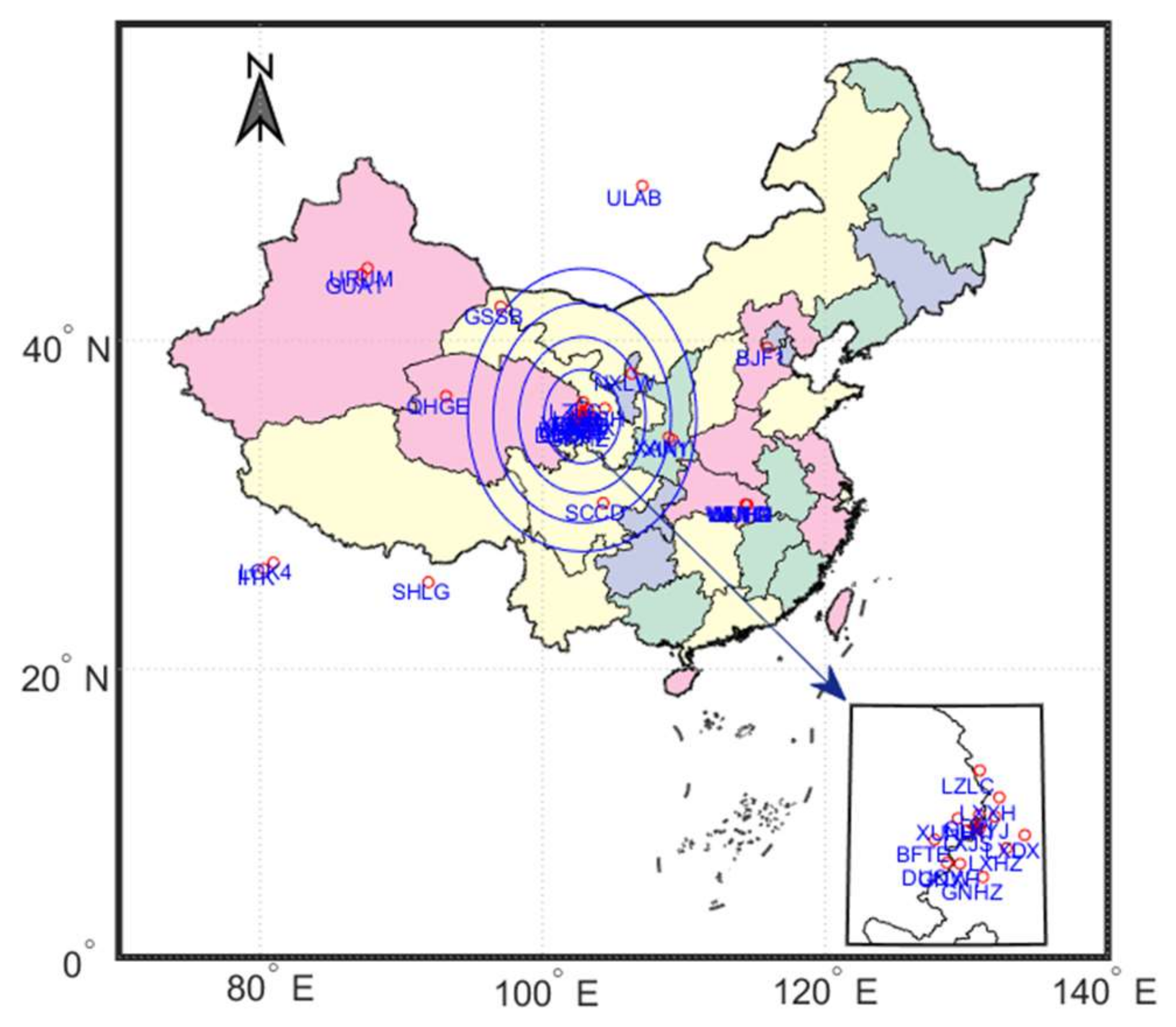
Figure 3.
Temporal evolution of spatial environmental parameters on the day of the Jishishan Earthquake.
Figure 3.
Temporal evolution of spatial environmental parameters on the day of the Jishishan Earthquake.
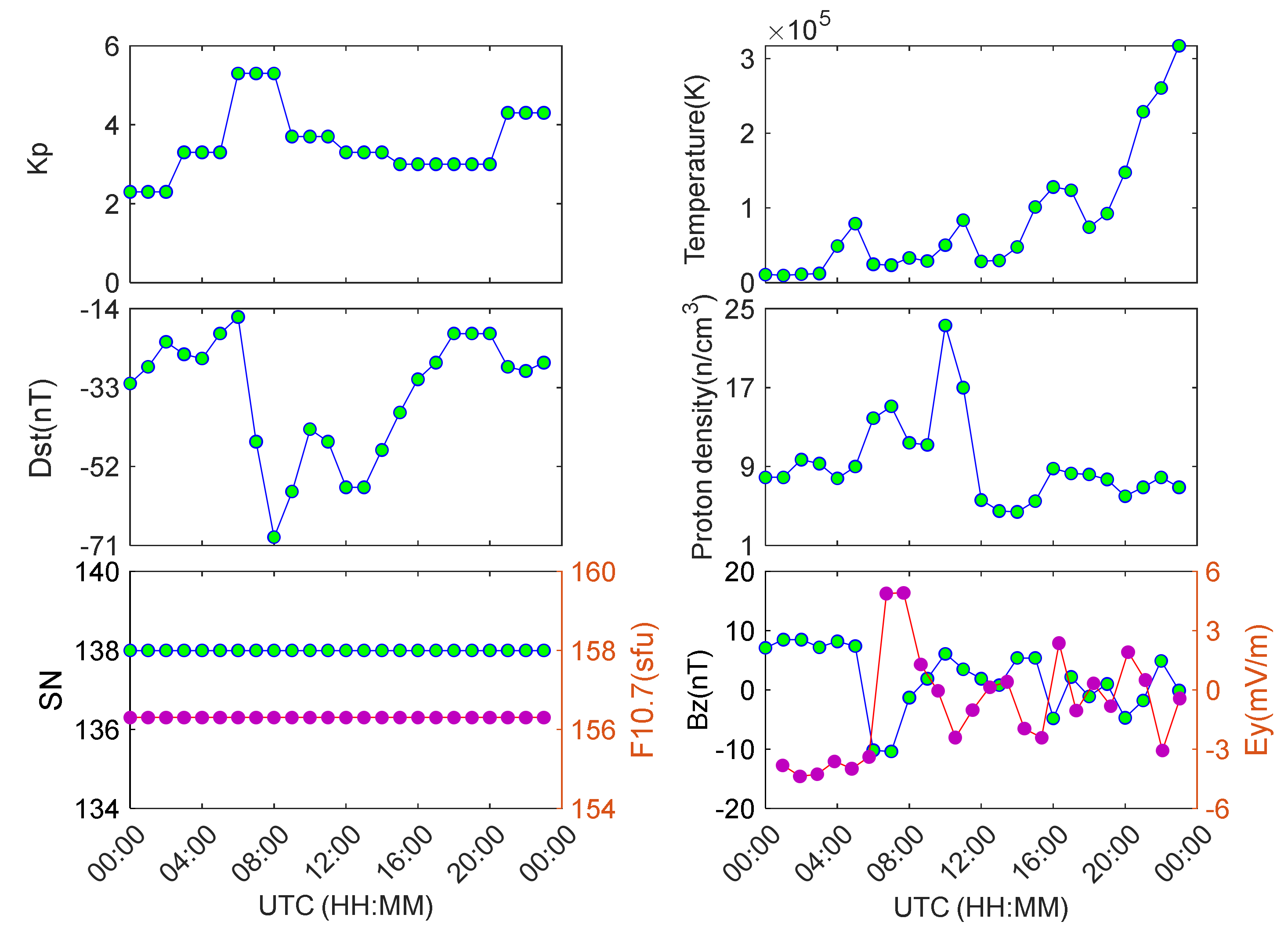
Figure 4.
Wavelet power spectral density of TEC time-series from BDS GEO satellites (C01–C03) at station LXJS, highlighting the spectral energy partitioning across frequency bands.
Figure 4.
Wavelet power spectral density of TEC time-series from BDS GEO satellites (C01–C03) at station LXJS, highlighting the spectral energy partitioning across frequency bands.
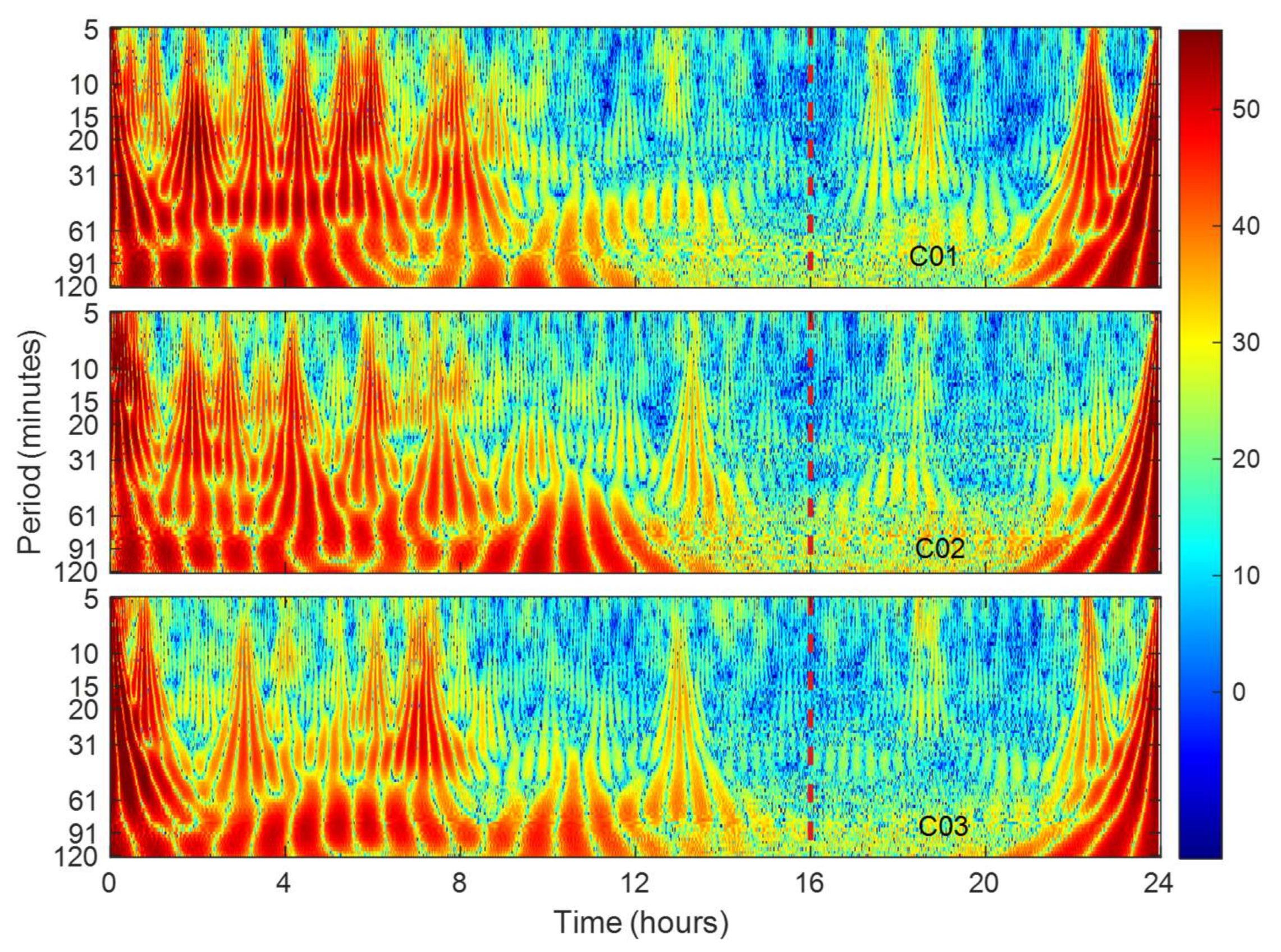
Figure 5.
The DTEC time series derived from dual-frequency BDS GEO satellite observations at station LXJS (left: C02; right: C03).
Figure 5.
The DTEC time series derived from dual-frequency BDS GEO satellite observations at station LXJS (left: C02; right: C03).
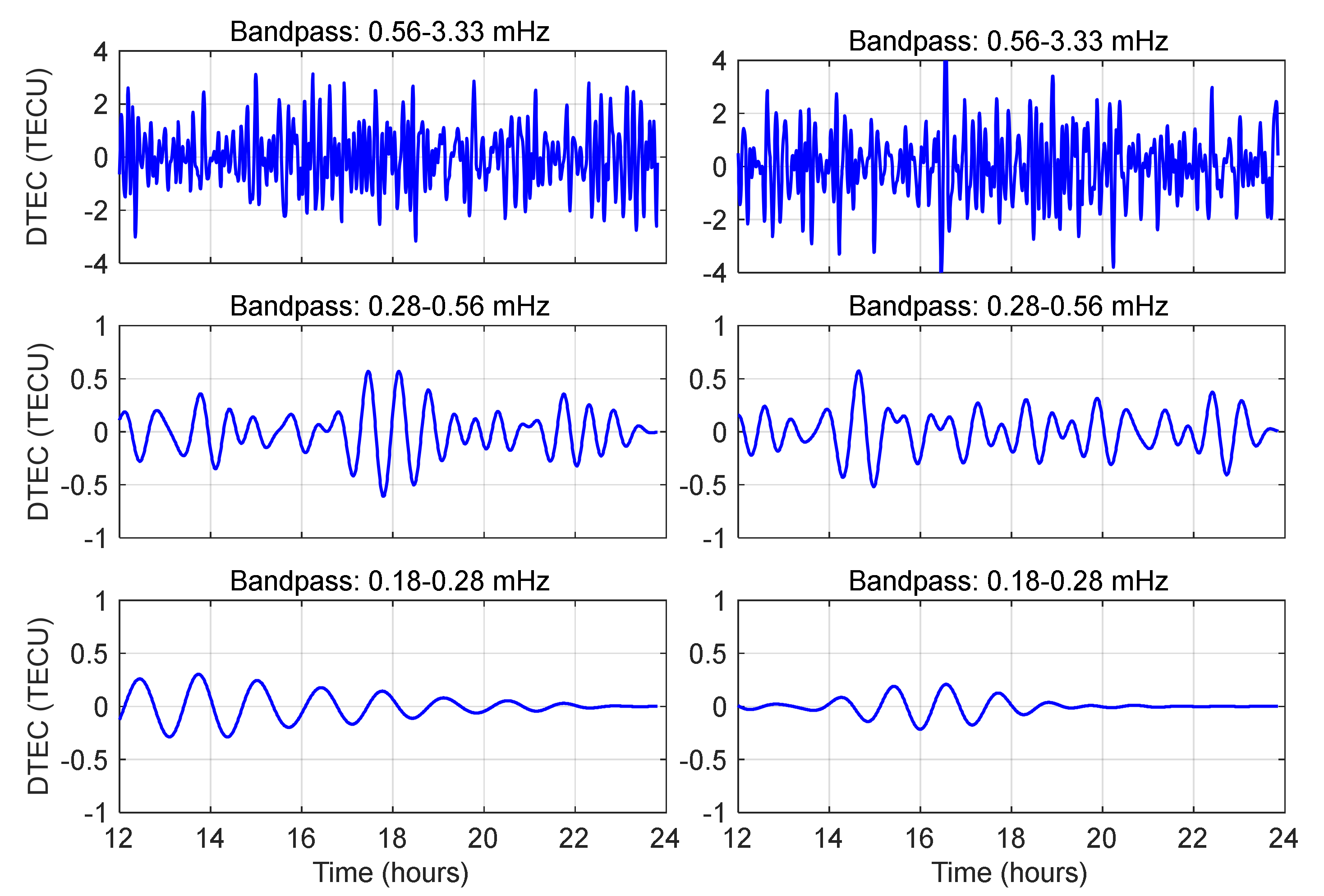
Figure 6.
The DTEC time series derived from dual-frequency BDS GEO satellite observations at station LXHZ (left: C02; right: C03).
Figure 6.
The DTEC time series derived from dual-frequency BDS GEO satellite observations at station LXHZ (left: C02; right: C03).
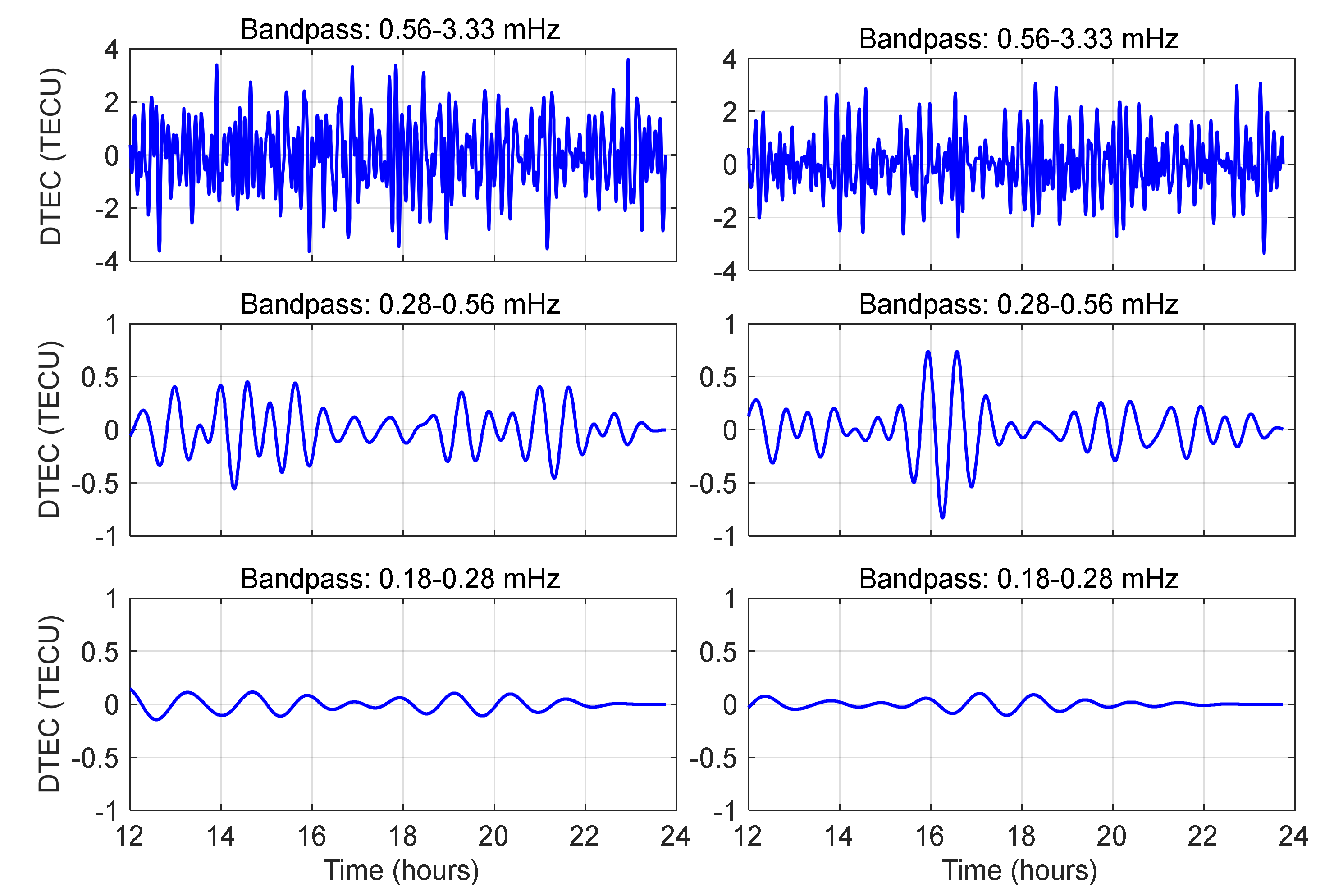
Figure 7.
The DTEC time series derived from dual-frequency BDS GEO satellite observations at station LXSH (left: C02; right: C03).
Figure 7.
The DTEC time series derived from dual-frequency BDS GEO satellite observations at station LXSH (left: C02; right: C03).
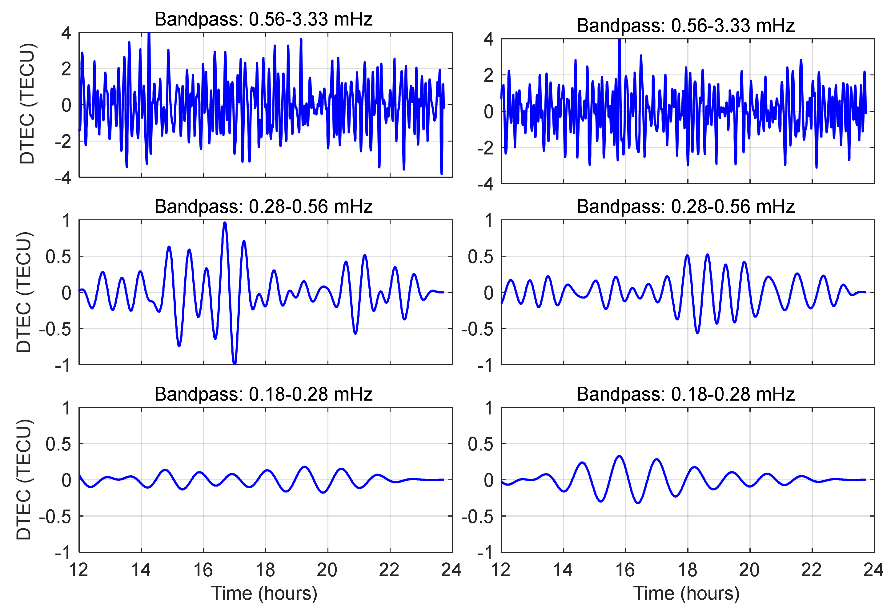
Figure 8.
The DTEC time series derived from dual-frequency BDS GEO satellite observations at station BJF1 (left: C02; right: C03).
Figure 8.
The DTEC time series derived from dual-frequency BDS GEO satellite observations at station BJF1 (left: C02; right: C03).
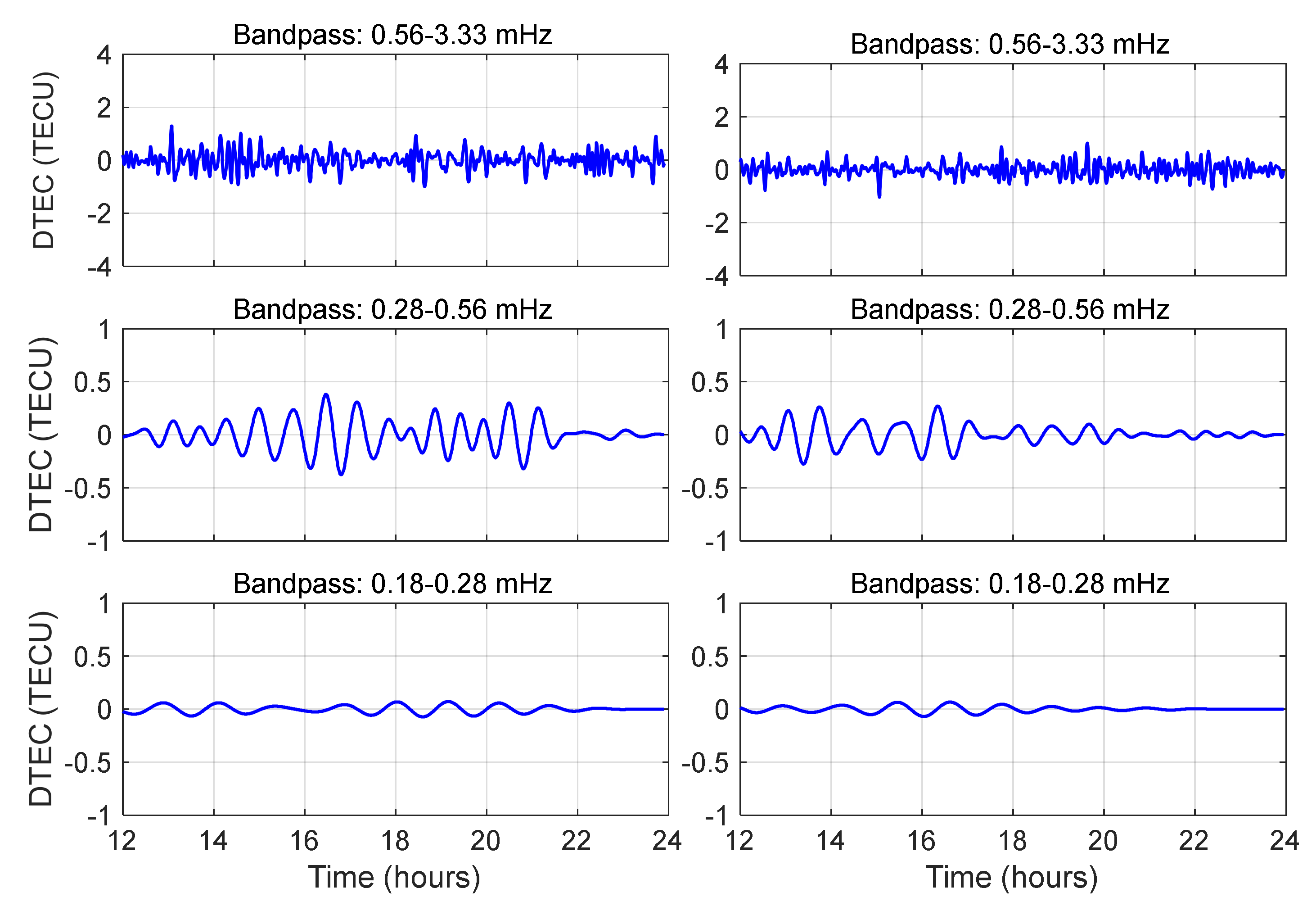
Figure 9.
DTEC travel-time variations and IPP distributions for satellite C02 (cut-off frequency: 0.56–3.33 mHz).
Figure 9.
DTEC travel-time variations and IPP distributions for satellite C02 (cut-off frequency: 0.56–3.33 mHz).
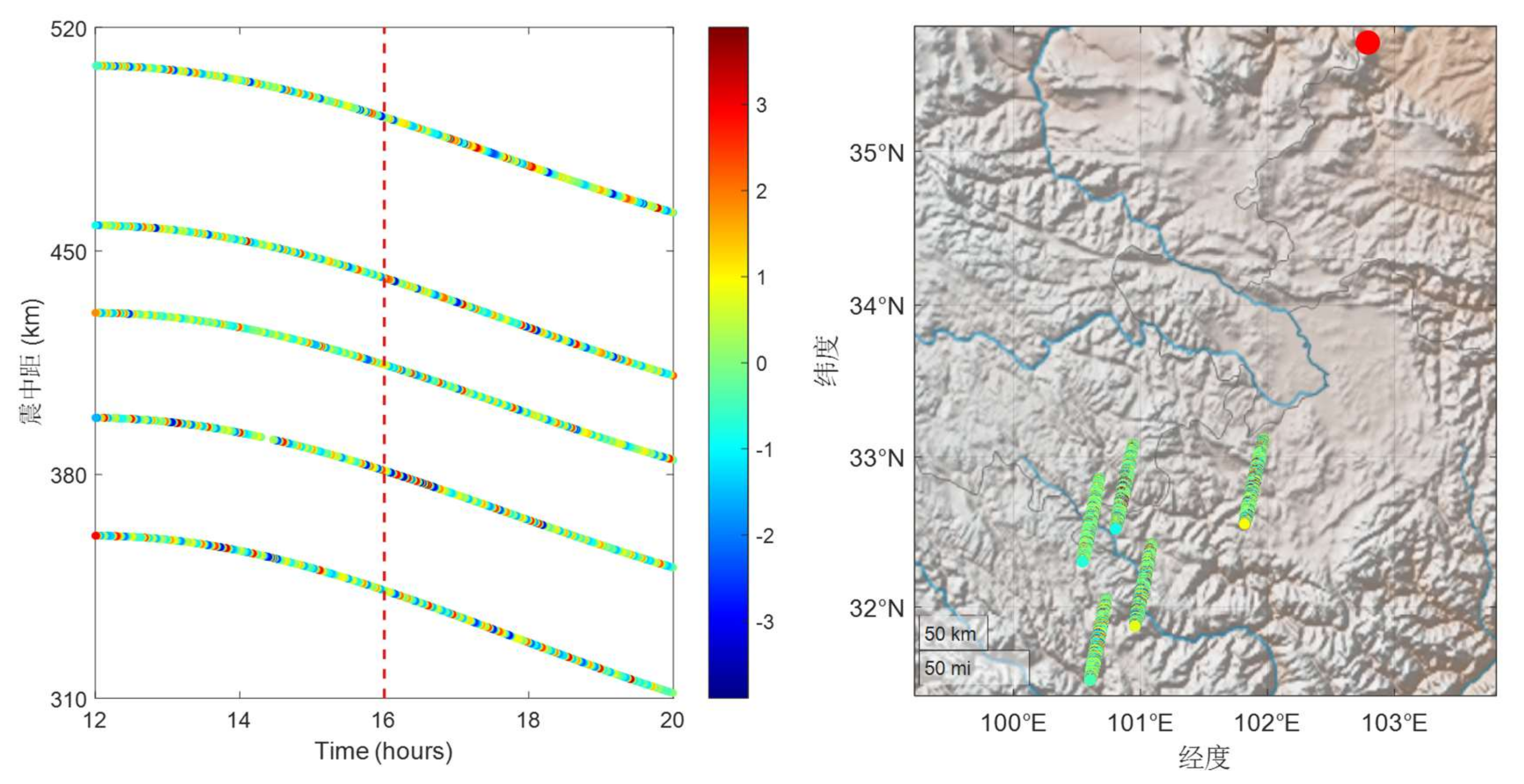
Figure 10.
DTEC travel-time variations and IPP distributions for satellite C02 (cut-off frequency: 0.28–0.56 mHz).
Figure 10.
DTEC travel-time variations and IPP distributions for satellite C02 (cut-off frequency: 0.28–0.56 mHz).
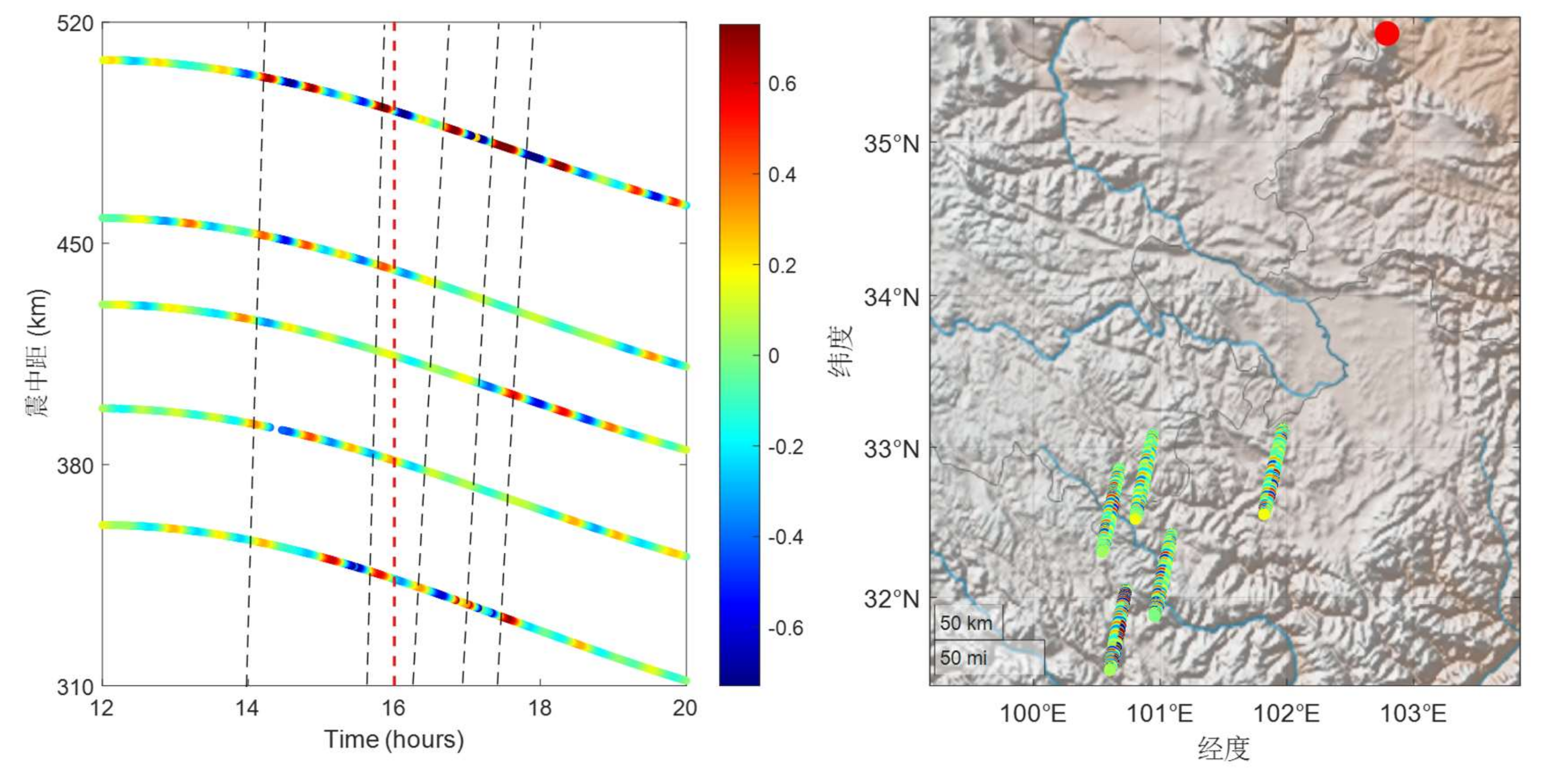
Figure 11.
DTEC travel-time variations and IPP distributions for satellite C02 (cut-off frequency: 0.18–0.28 mHz).
Figure 11.
DTEC travel-time variations and IPP distributions for satellite C02 (cut-off frequency: 0.18–0.28 mHz).
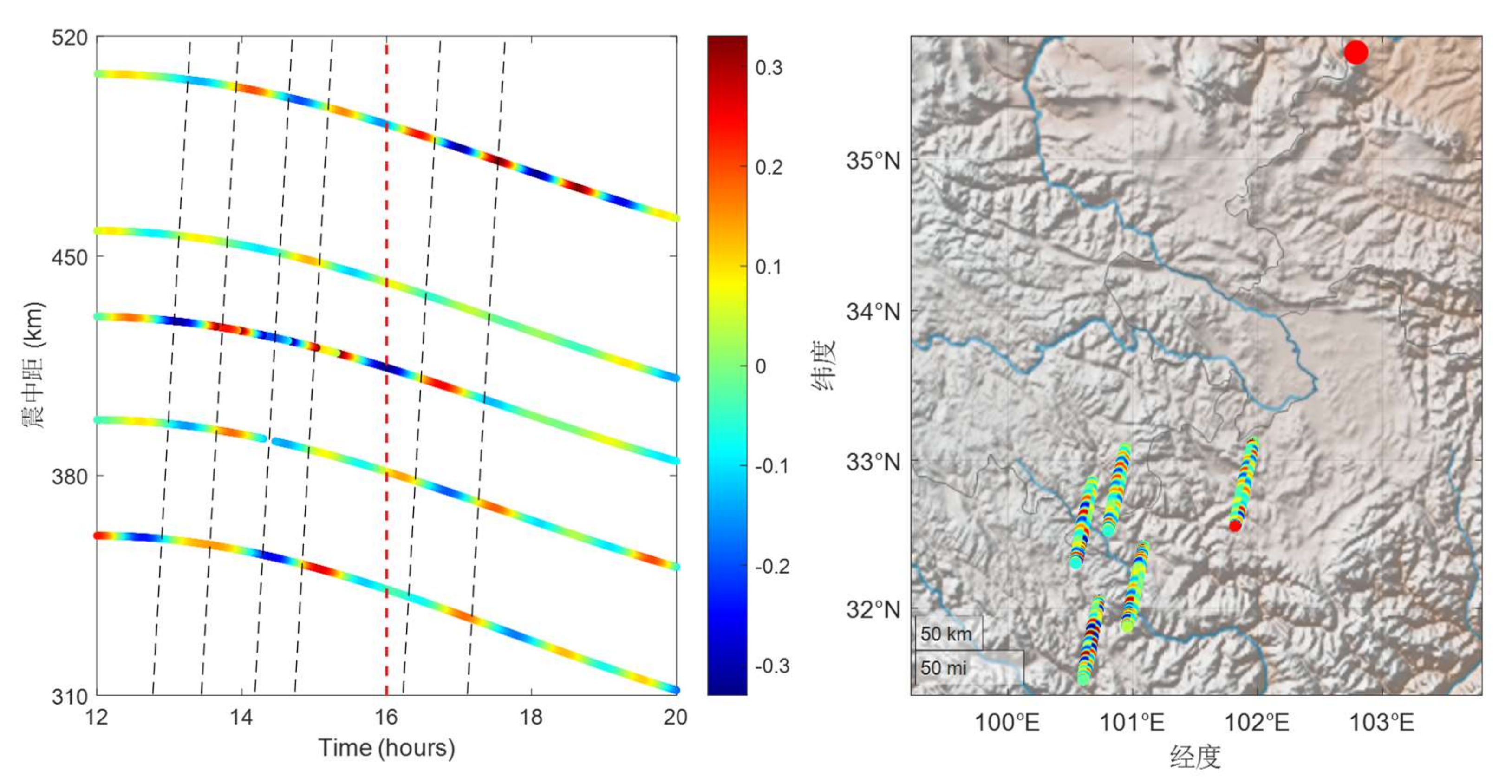
Figure 12.
DTEC series at LZJS station during the minor geomagnetic storm on the earthquake day (left: C02; right: C03).
Figure 12.
DTEC series at LZJS station during the minor geomagnetic storm on the earthquake day (left: C02; right: C03).
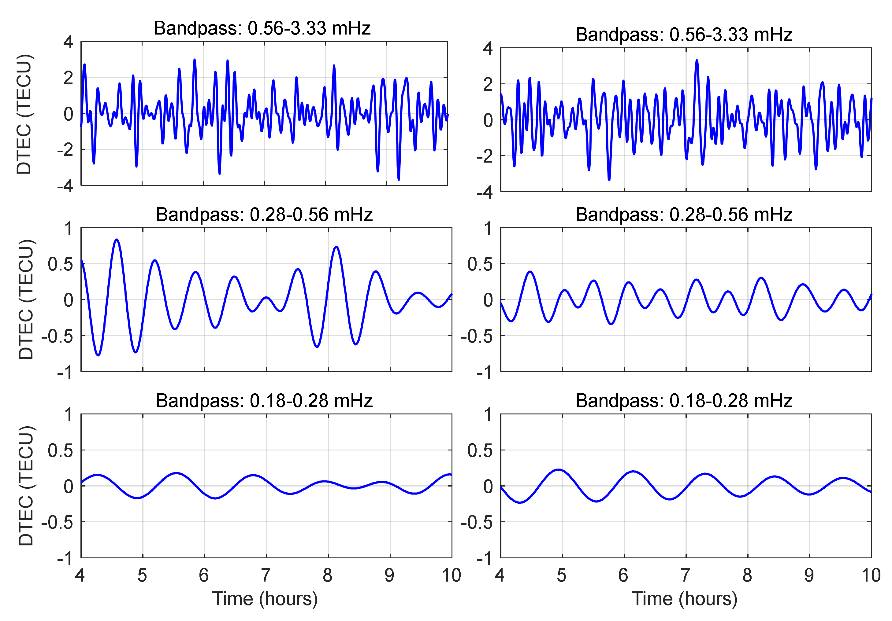
Figure 13.
DTEC series at LZHZ station during the minor geomagnetic storm on the earthquake day (left: C02; right: C03).
Figure 13.
DTEC series at LZHZ station during the minor geomagnetic storm on the earthquake day (left: C02; right: C03).
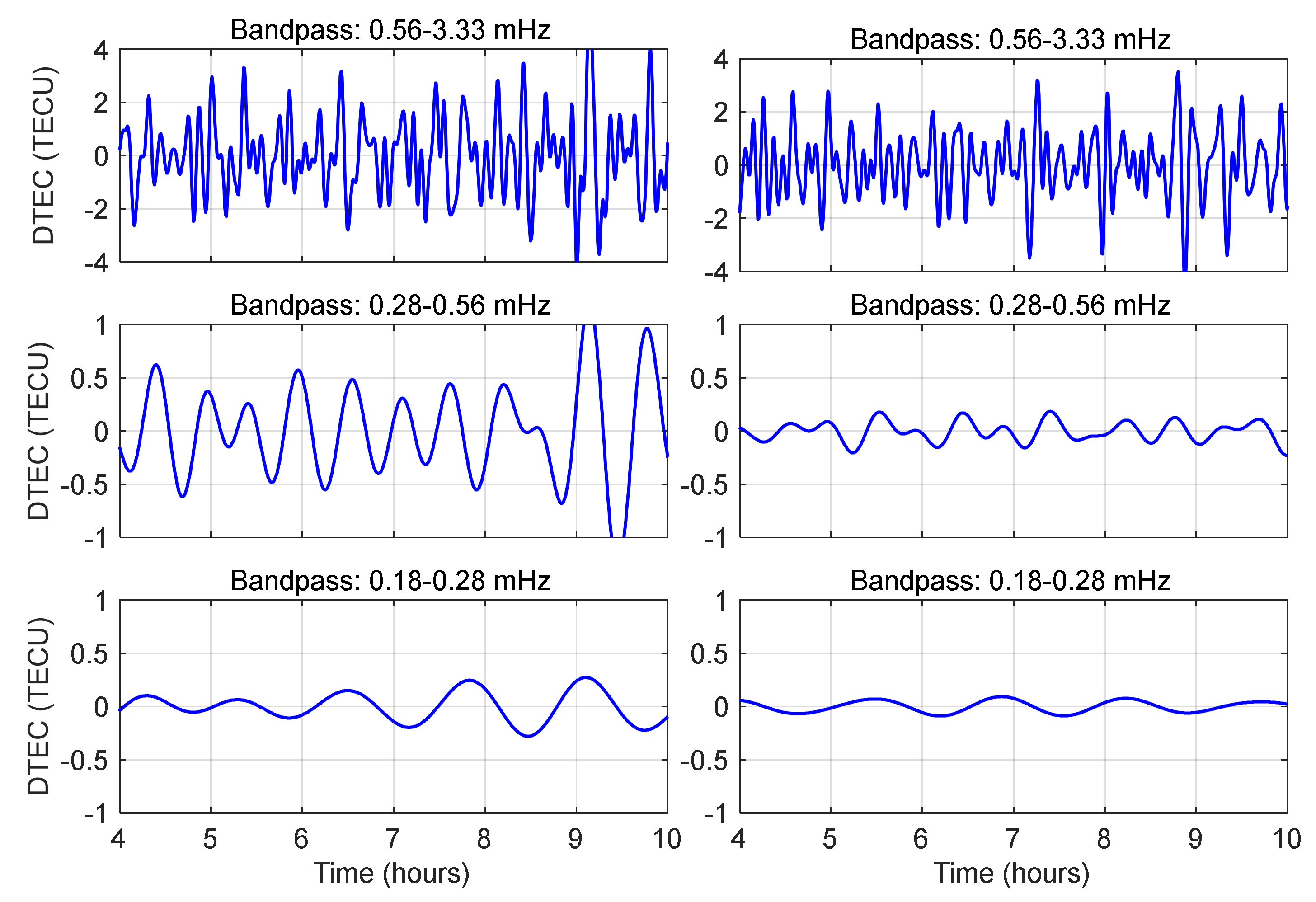
Figure 14.
DTEC series at LZSH station during the minor geomagnetic storm on the earthquake day (left: C02; right: C03).
Figure 14.
DTEC series at LZSH station during the minor geomagnetic storm on the earthquake day (left: C02; right: C03).
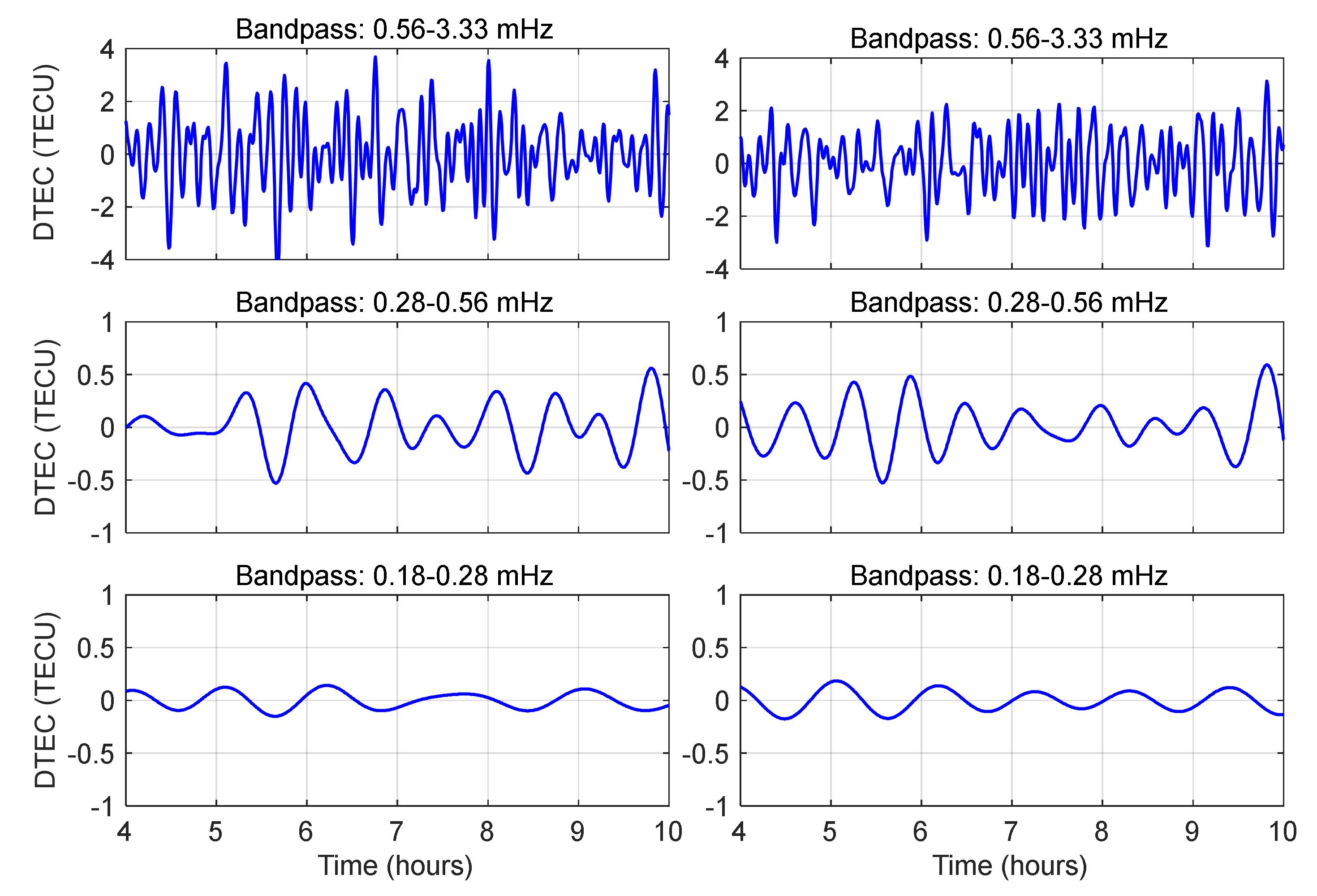
Figure 15.
Time series of DTEC at BJF1 station during the minor geomagnetic storm on the earthquake day (left: C02; right: C03).
Figure 15.
Time series of DTEC at BJF1 station during the minor geomagnetic storm on the earthquake day (left: C02; right: C03).
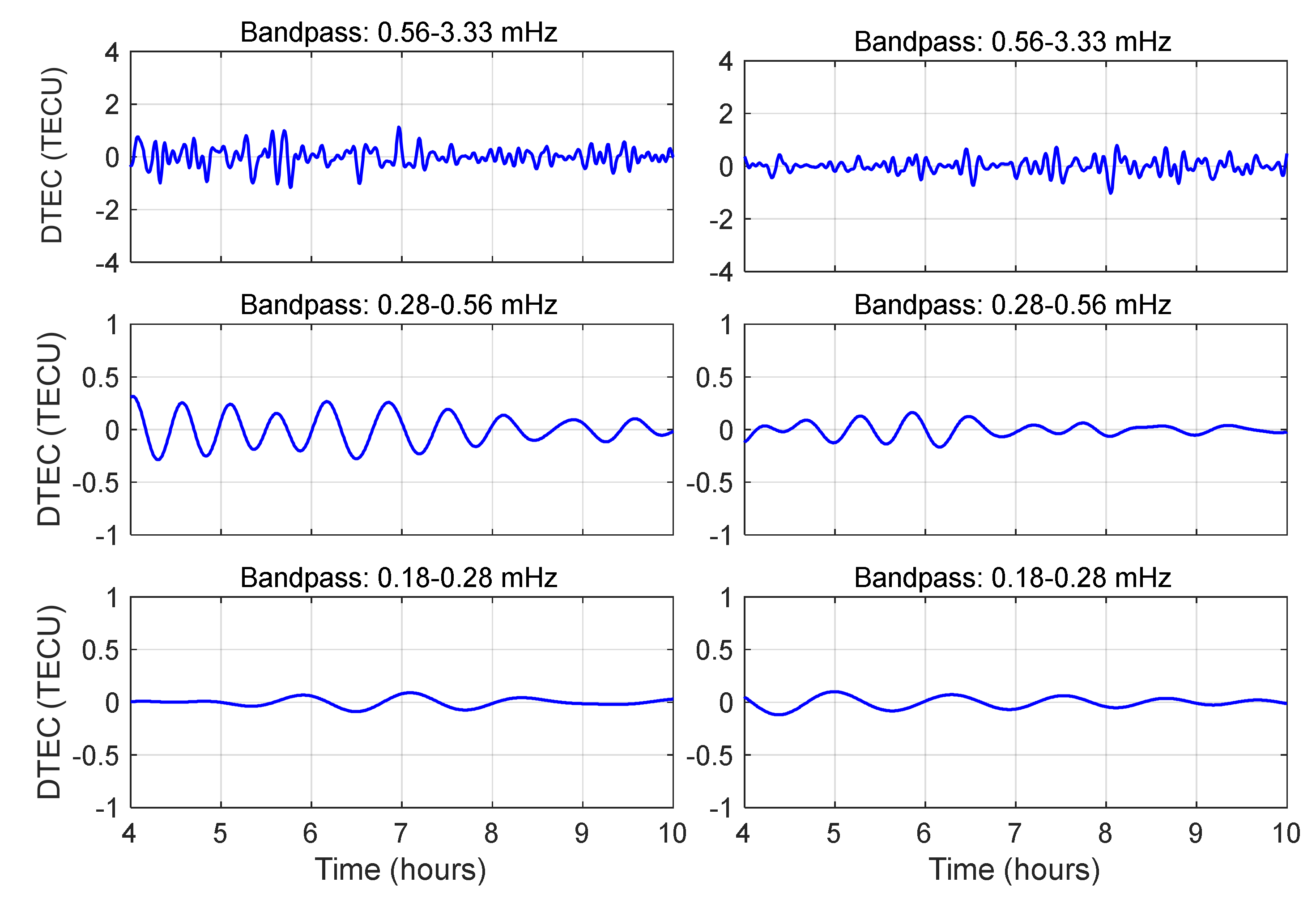
Figure 16.
Travel-time diagrams of TEC perturbations across azimuthal sectors (left: C02; right: C03; Cut-off frequency: 0.56–3.33 mHz, corresponding to 5–30 min Periods).
Figure 16.
Travel-time diagrams of TEC perturbations across azimuthal sectors (left: C02; right: C03; Cut-off frequency: 0.56–3.33 mHz, corresponding to 5–30 min Periods).
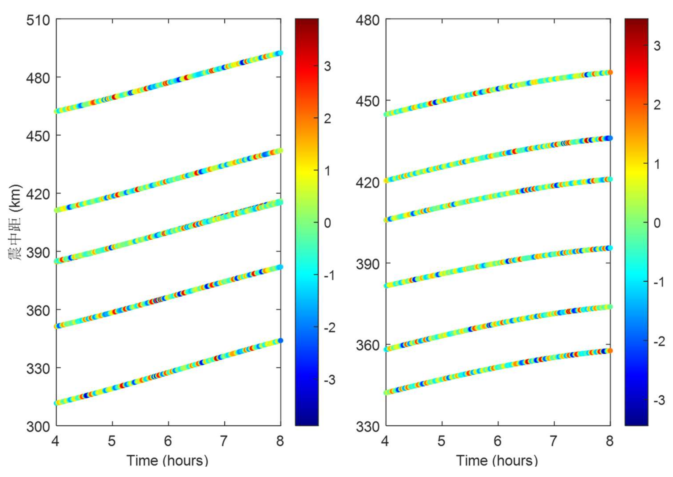
Figure 17.
Travel-time diagrams of TEC perturbations across azimuthal sectors (left: C02; right: C03; Cut-off frequency: 0.28–0.56 mHz, corresponding to 30–60 min Periods).
Figure 17.
Travel-time diagrams of TEC perturbations across azimuthal sectors (left: C02; right: C03; Cut-off frequency: 0.28–0.56 mHz, corresponding to 30–60 min Periods).
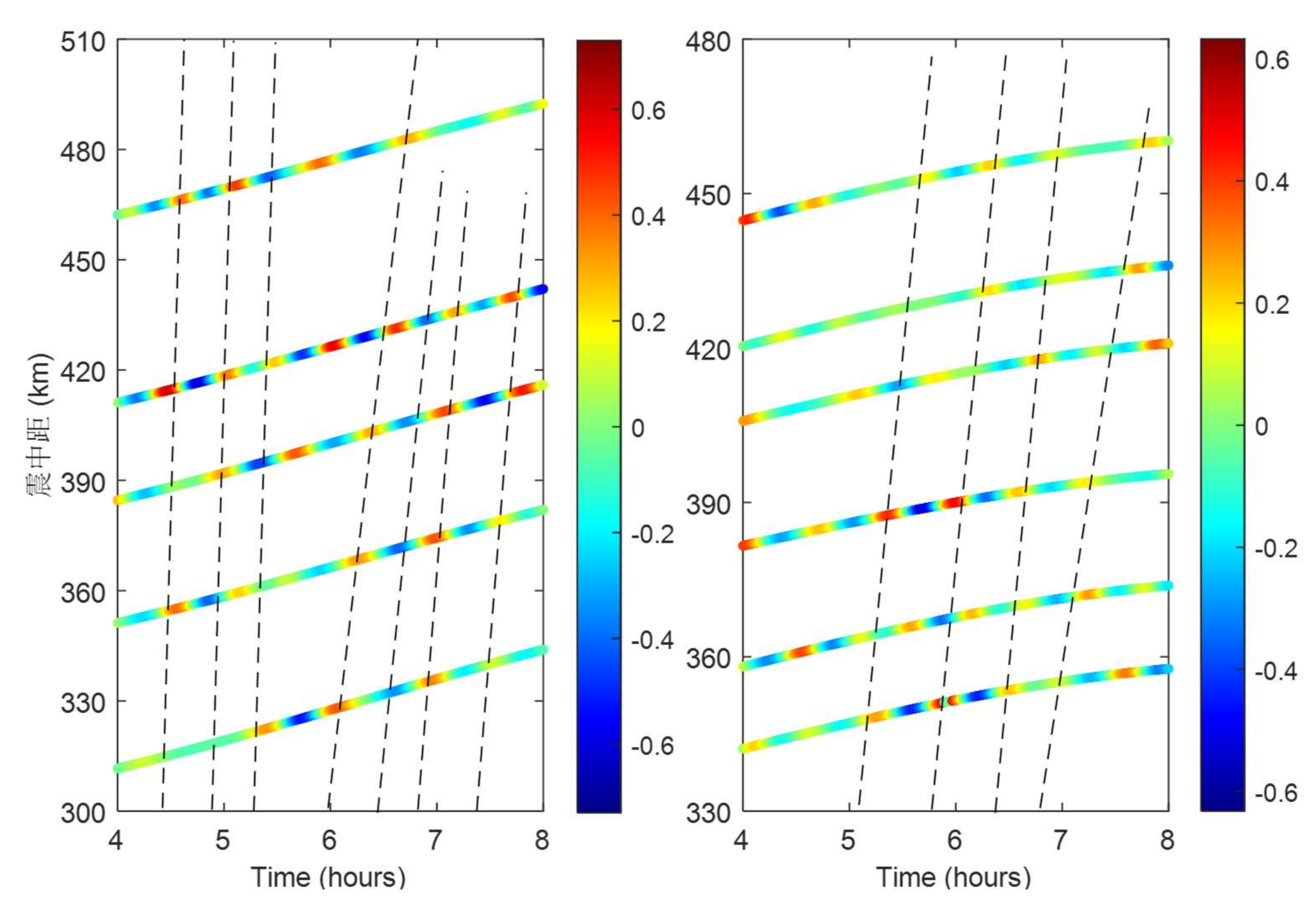
Figure 18.
Travel-time diagrams of TEC perturbations across azimuthal sectors (left: C02; right: C03; Cut-off frequency: 0.18–0.28 mHz, corresponding to 60–90 min Periods).
Figure 18.
Travel-time diagrams of TEC perturbations across azimuthal sectors (left: C02; right: C03; Cut-off frequency: 0.18–0.28 mHz, corresponding to 60–90 min Periods).
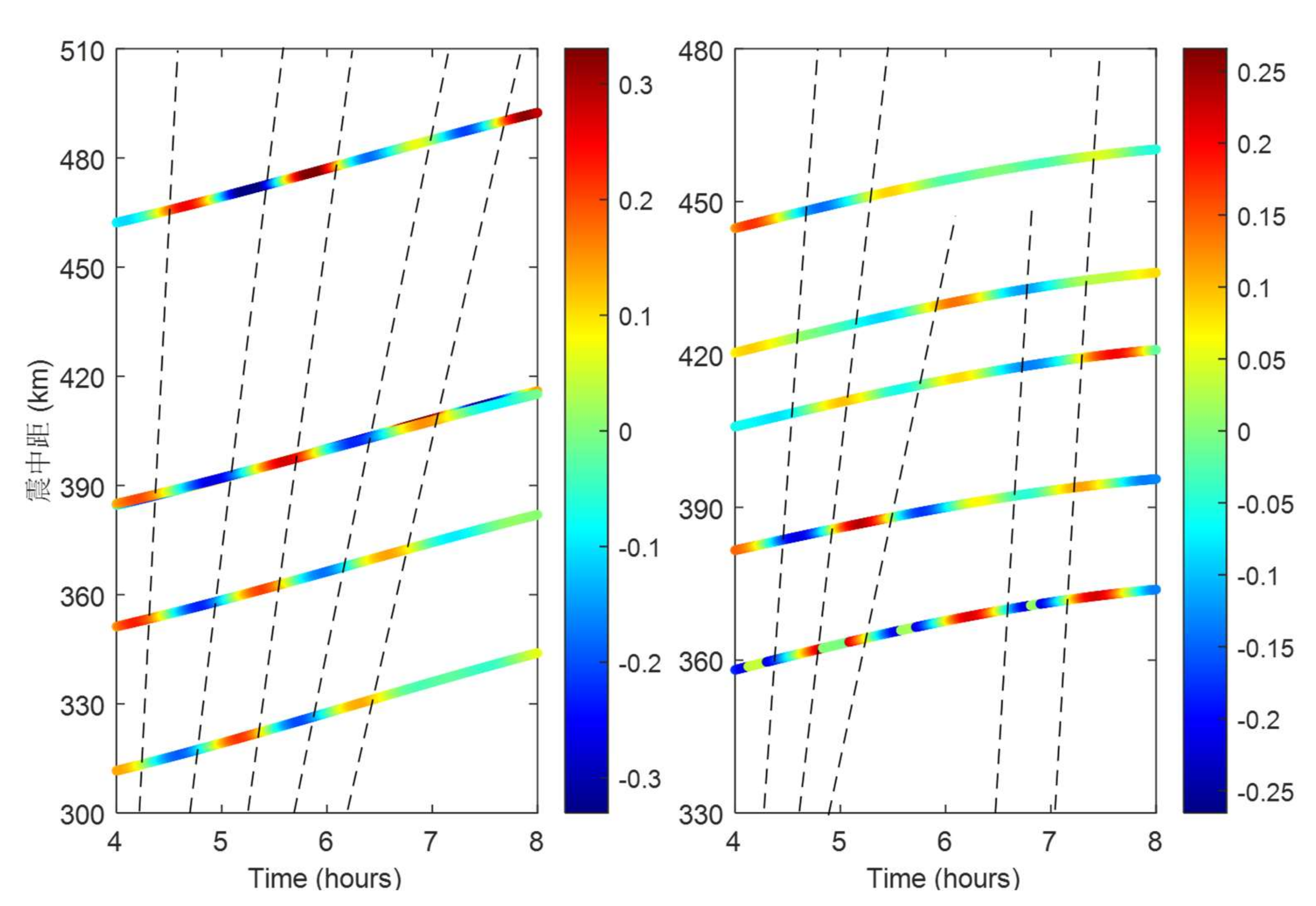

Table 1.
Seismicity catalog of Mw≥5.5 events within the Jishishan earthquake zone (2019–2025).
| Date | Time (UTC) |
Latitude 1 (°N) | Longitude (°E) |
Depth 2 (km) |
Mw | Type 3 |
|---|---|---|---|---|---|---|
| 2025/01/08 | 07:44:22.703 | 34.7612 | 97.4769 | 10 | 5.5 | mww |
| 2024/03/07 | 10:06:30.797 | 33.5389 | 92.9927 | 10 | 5.6 | mww |
| 2023/12/18 | 15:59:30.352 | 35.7386 | 102.8149 | 12 | 6.0 | mww |
| 2022/11/10 | 05:01:05.611 | 28.3835 | 94.4118 | 15 | 5.5 | mww |
| 2022/09/05 | 04:52:19.645 | 29.6786 | 102.236 | 12 | 6.6 | mww |
| 2022/08/14 | 08:20:00.340 | 33.1157 | 92.7977 | 5 | 5.7 | mww |
| 2022/06/09 | 17:28:35.801 | 32.3726 | 101.8721 | 7 | 5.9 | mww |
| 2022/06/09 | 16:03:26.522 | 32.3152 | 101.8363 | 10.14 | 5.6 | mww |
| 2022/06/01 | 09:00:08.401 | 30.3951 | 102.9582 | 12 | 5.8 | mww |
| 2022/03/25 | 16:21:03.998 | 38.5365 | 97.2898 | 10 | 5.7 | mww |
| 2022/01/23 | 02:21:19.926 | 38.4613 | 97.3425 | 10 | 5.6 | mww |
| 2022/01/07 | 17:45:30.809 | 37.8283 | 101.29 | 13 | 6.6 | mww |
| 2021/06/16 | 08:48:58.863 | 38.2061 | 93.7234 | 10 | 5.5 | mww |
| 2021/05/21 | 18:13:01.128 | 34.4808 | 99.0805 | 10 | 5.5 | mb |
| 2021/05/21 | 18:12:15.048 | 34.617 | 98.4674 | 10 | 5.5 | mb |
| 2021/05/21 | 18:04:13.565 | 34.5983 | 98.2513 | 10 | 7.3 | mww |
| 2021/05/21 | 13:48:37.193 | 25.7274 | 100.0082 | 9 | 6.1 | mww |
| 2021/03/19 | 06:11:27.113 | 31.9246 | 92.9151 | 8 | 5.7 | mww |
1 Magnitude types: moment magnitude, denoted as “mww” in USGS catalog, mb (body-wave magnitude). 2 Depth: Hypocentral depth rounded to one decimal place. 3 Coordinate precision: Locations reported in decimal degrees (WGS84).
Table 2.
Spatial evolution of ionospheric disturbances (DTEC) across frequency bands and epicentral distances (Unit: TECU)..
Table 2.
Spatial evolution of ionospheric disturbances (DTEC) across frequency bands and epicentral distances (Unit: TECU)..
| Station Parameters | LXJS (5.2km ) | LXHZ (59.7km ) |
LZSH (151.6km ) |
BJF1 (1220km ) |
|
|---|---|---|---|---|---|
| Bandpass 0.56-3.33mHz |
Max-Min | 9.2824 | 8.5380 | 9.2968 | 2.0349 |
| STD | 1.1304 | 1.1465 | 1.1728 | 0.2461 | |
| Bandpass 0.28-0.56mHz |
Max-Min | 1.8820 | 2.7855 | 1.3808 | 0.7466 |
| STD | 0.2186 | 0.2463 | 0.2195 | 0.0968 | |
| Bandpass 0.18-0.28mHz |
Max-Min | 2.6155 | 2.0146 | 0.7763 | 0.4660 |
| STD | 0.2517 | 0.1914 | 0.1181 | 0.0590 | |
Disclaimer/Publisher’s Note: The statements, opinions and data contained in all publications are solely those of the individual author(s) and contributor(s) and not of MDPI and/or the editor(s). MDPI and/or the editor(s) disclaim responsibility for any injury to people or property resulting from any ideas, methods, instructions or products referred to in the content. |
© 2025 by the authors. Licensee MDPI, Basel, Switzerland. This article is an open access article distributed under the terms and conditions of the Creative Commons Attribution (CC BY) license (http://creativecommons.org/licenses/by/4.0/).
Copyright: This open access article is published under a Creative Commons CC BY 4.0 license, which permit the free download, distribution, and reuse, provided that the author and preprint are cited in any reuse.


