
Submitted:
18 November 2025
Posted:
19 November 2025
You are already at the latest version
Abstract
With air resistance being one of the two major energy losses in on-road vehicles (the other one being tire losses) and therefore heavily contributing to the range of battery-electric and fuel cell-electric vehicles, it is necessary to account for realistic air resistance in a-priori assessments like vehicle range esti-mations, component dimensioning, and system simulations. However, lack of input data tempts analysts to instead assume unrealistic “nom-inal conditions” throughout – a simplification which usually underestimates the amount of energy actually required to overcome air resistance and completely ignores the fact that varying environmental conditions will lead to significant variances in energy consumption and therefore vehicle range. Using “nominal conditions” it is thus impossible to assess the robustness of these measures and therefore difficult to design robust systems and to perform meaningful trade-off studies. In this study we show how publicly available data from weather observations can be used to assess the long-term variation of air resistance of a truck with semitrailer. Realistic distributions of energy losses due to air resistance, covering multiple years are derived – showing not only average values but the complete envelope in which the energy losses vary. This, in turn, enables to follow up with probabilistic calculations of vehicle per-formance in order to assess robustness and trade-offs on various system levels of interest. As a consequence consumption and range predictions of EVs and ICE vehicles can be performed with higher accuracy and confidence.
Keywords:
vehicle range prediction
; environmental losses
; energy consumption
; energy losses
; air resistance
; air drag
; weather data
; meteorological observations
; recorded weather
1. Introduction
In any moving machine or vehicle a significant amount of energy is lost due to interaction with the environment [1,2,3,4,5,6]. The contribution of air drag to the total amount of energy required is reported as 20% in [1], 15-45% in [3], and 38% in [5]. While in on-road vehicles powered by internal combustion engines (ICEs) a significant amount of energy is also lost in the ICE itself [3], in vehicles with energy-efficient powertrains, such as battery-electric vehicles (BEVs), the energy losses due to environmental interaction clearly dominate [4]. These losses negatively affect vehicle range and therefore influence how much battery capacity is required to fulfil intended specifications.
The desire to virtually guarantee a certain vehicle range, despite variations in environmental conditions, quickly leads to over-dimensioning of the on-board battery storage – even more so when the envelope, within which environmental conditions can vary, and the associated statistical distribution is unclear. Since battery is a major cost factor in any BEV, it is of great interest to be able to reliably quantify a vehicle’s environmental losses in operation.
While in off-road machines the environmental interactions include performing actual work on the environment, like filling a bucket of an excavator or a wheel loader [2], in on-road vehicles the environmental interactions are only due to the vehicle moving on the road and through the air [1,3,4,5,6]:
- changes in elevation;
- rolling resistance due to tire losses;
- aerodynamic resistance due to air drag.
The latter two items are non-recoverable losses. The Drag-Dominant Speed, DDS, according to [7] marks the vehicle speed where a vehicle’s air resistance equals its tire losses. Above DDS air resistance dominates and increases quickly as it is proportional the vehicle speed squared. In the example pictured in Figure 1 the DDS of a 40 ton truck can be found as the intersection of the curves at 76 km/h (computed using the following input data: = 0.004, = 5.772, = 1.225).
2. Air resistance
Typically, air resistance is modelled as in Equation 1.
This simple equation exposes that the drag force is quadratically dependent on the vehicle speed but varies only linearly with air density , the vehicle’s drag coefficient and its cross-section .
In reality wind adds to the ram air such that instead of vehicle speed the total airflow must be considered. Also, both factors of the product are dependent on the angle of the attacking airflow, thus the relative wind direction , which is the absolute wind direction relative to the moving vehicle’s heading , matters (see Figure 2).
Airflow being the vector sum of vehicle speed and wind is hardly a new insight. Lack of vehicle data to properly account for the effect of the crosswind component can be one of the reasons why it is sometimes neglected. For competitive reasons vehicle manufacturers are hesitant to disclose values, especially for other airflow angles than 0° and academic researchers having obtained such data guard it as a close secret. In this regard paper [8] is a noticeable and welcome exception.
Other input to Equation 1, not readily available for most researchers is realistic data on the movement and density of the air (typical values or comprehensive distributions for wind speed and direction, air temperature, air pressure, humidity, precipitation). There are attempts to achieve more realistic results by means of Wind-Averaged Drag (WAD) analysis [9,10,11] in which a simplified yaw angle weighting function is featured – although constant wind speed is assumed. In paper [12] both wind direction and wind speed are used as an improvement, but still this is a simplification.
In any case, finding a WAD value that is representative for all locations in the world is impossible. In our work, as initially reported in [13], we therefore instead utilize quality-assured data from meteorological observations conducted and published by various national and international authorities. This results in the correct distribution for any variable desired: wind speed and direction, air temperature, air humidity etc.
Using observed weather data is not novel in traffic safety research, for example for automated driving [14,15] or in the forecast of operational performance of renewable energy systems [16]. However, no literature can be found that show how such data from long-term observations can be used at large scale and processed efficiently to augment the logged data from moving vehicles and/or to analyze energy losses in realistic and representative way. This is where the contribution of our work lies, with the specific study presented in this paper focusing only on air resistance.
3. Study Setup
3.1. Vehicle Parameters
We have chosen to consider a tractor with semitrailer in our study. In order to not disclose any vehicle parameters related to aerodynamics, again: competitive reasons, we have chosen to utilize data from [8] and [1], reprocessed to fit our purpose (see Figure 3).
Note that for airflow angles values above the is negative, meaning that due to a sailing effect the airflow helps propelling the vehicle forward, rather than resisting the movement. To provide a reference, in order to get an airflow angle of 72° a vehicle moving at 90 km/h would need to be exposed to a 90° crosswind of 270 km/h.
Figure 4 shows the relationship between wind and airflow, in terms of angle and speed, for a vehicle moving with a speed of 50 km/h and 90 km/h. It is clear that high airflow angles require unusual high wind speeds even at a mere 50 km/h vehicle speed – at which the actual drag force acting on the vehicle is small. We can thus conclude that the sailing effect has likely no significant impact in reality.
See also Figure 10 which shows the airflow encountered by the simulated vehicles over the course of 5 years: it is confirmed that airflow angles above 20° are incredibly rare and angles above 35° are virtually non-existent.
3.2. Representative Driving Cycles
The method described in [13] requires a time series of global coordinates, such as recorded with GNSS. In the study presented here the aim was to analyze air resistance in a way that expresses the vehicle’s general properties, which means it cannot be tied to a specific track at a specific time.
We have therefore chosen to analyze an ensemble of various tracks, run twice a day over a period of 5 years, thereby reducing location and time dependency in the results. This required to handle a significant amount of data.
Due to reasons described in [13] we have utilized weather observations in Sweden. We have generated artificial driving logs for 11 routes in southern Sweden (see Figure 5), to be driven in both directions, thus 22 tracks in total. A combination of respective APIs from HERE and Google Maps have been used to create high-resolution synthetic GNSS logs that adhere to typical traffic speeds and the legal speed limits (although the software developed makes it possible to limit to a speed lower than the legal limit).
This ensemble of tracks has then been run twice a day. The time vectors have been constructed so that in the morning the simulated vehicles start collectively at 06:00 Z (i.e., local time, taking daylight saving into account) and arrive individually according to the conditions of their respective track, while in the evening the vehicles are made to arrive collectively at 18:00 Z, which means they start individually at the time required to finish their respective journey at precisely 18:00 Z.
3.3. Long-Term Data from Weather Observations
The aforementioned ensemble of tracks has then been run twice a day, every day, over 5 years from January 1st, 2018 to December 31st, 2022. Table 1 lists which data have been extracted from recorded weather observations for each individual log position.
As can be seen we have utilized two data providers, the Swedish Meteorological and Hydrological Institute (SMHI) and the Swedish Transport Authority, Trafikverken (TrV). The latter has graciously provided us with data from their long-term archive of the Road Weather Information System, Vägväderinformationssystem (VViS).
However, the VViS bins values for wind direction into only 8 bins, corresponding to the general directions N, NE, E, SE, S, SW, W, and NW. We compared a year of saved high-resolution data from TrV’s REST API (with wind direction in the interval from 0° to 359° in steps of 1°) for the period from September 1st, 2023 to August 31st, 2024 to the corresponding data from the VViS archive in order to ascertain that the latter give relevant results despite the lower resolution of wind direction. Figure 6 shows that there are deviations mainly in the interval of ±5% but with a rather tight and symmetric distribution.
The reason for using VViS data is that we have considerably more data available. Our study started in August 2023, meaning that at the time of writing we only have 2 years of high-resolution data from the REST API – compared to the 16 years of data that Trafikverket graciously provided us with.
To keep computation time reasonable we have used 5 years of the VViS and SMHI data to augment each synthetic GNSS log point in each track with data as listed in Table 1, twice a day, all days from January 1st, 2018 to December 31st, 2022. Extraction with Matlab using 6 of 8 CPU cores took about 190 hours on PC with an i7-7800X CPU and 16GB RAM.
Figure 7 shows an example of a simulated vehicle travelling from Örebro to Göteborg on October 1st, 2023 starting at 12:00 Z. The blue dots are the TrV meteo stations used to extract data for air temperature, wind speed and wind direction. The grey rings are plotted to show the road sections corresponding to each meteo station. The plots of spatial and temporal error show that the extracted data matches the vehicles position in space and time as well as can be demanded: the data is never more than 5 minutes old (in either direction) and often from a location less than 10 km away from the vehicle.
In comparison, Figure 8 shows the situation for air pressure extracted from the SMHI database: the corresponding meteo stations are more sparsely distributed and deliver data only once an hour, which leads to larger spatial and temporal errors than which is the case for data from the TrV stations. However, this is acceptable because the local variance of air pressure is typically low.
Figure 9 shows the situation for air humidity extracted from the SMHI database. It can be seen that the software chooses slightly different meteo stations than for air pressure. One reason is that in contrast to TrV’s stations which all are equipped in the same way, the meteo stations of SMHI are not identical in terms of which sensors are available. Another reason can be that at the requested time the respective sensor might have been faulty or in maintenance, thus no data exists and the software had to choose data from another station farther away.
Also in this case we find larger spatial and temporal errors than which is the case for data from the TrV stations – but also here this is acceptable because while the local variance of air humidity can be higher than for air pressure, it is low nevertheless and the influence of the amount or water vapor in the air on air density is less than what is the case for air temperature and air pressure.
3.4. Calculations
According to Equation 1 we need air density , airflow speed , and the product to calculate the resistive force due to air drag.
We calculate air density from the recorded data for temperature, pressure and humidity of the air as per [17,18]. It should be noted that pressure data provided by SMHI (or any other meteorological service) are recalculated to mean sea level, yet required by us as pressure at road altitude. We use the Barometric Formula [19] for conversion, specifically the equation applicable to the atmospheric layers in which the temperature is assumed to vary with altitude at a non null temperature gradient.
The airflow speed and angle of attack are calculated as shown in Figure 2 – with the note that this requires to know the vehicle’s heading , which is computed in connection with generation of the synthetic vehicle logs.
Airflow angle is then used to derive from a lookup table containing the values shown in Figure 3.
Integration of the computed air drag force over time yields the energy required to overcome air resistance of the vehicle.
4. Results
Figure 10 shows the distribution of airflow in terms of speed and angle, that the vehicles have been subjected to, travelling at typical speed and not exceeding the specified or legal limit (in our study: limit set to 90 km/h). Previously we have elaborated that the sailing effect indicated by Figure 3 for airflow angles above 72° is likely to have no great significance in reality, which is now confirmed by the distributions shown in Figure 10: the vehicles rarely encounter airflow above 20° angle over the course of 5 years – and virtually never airflow above 35°.
The distributions shown in Figure 10 are already a much-desired result. We have previously discussed that researchers might refrain from including real wind, and especially crosswind into their calculations of air resistance because it might be unclear which values and probabilities to use. Figure 10 provides the values, representative for southern Sweden. These data can now be used in further calculations.
In our study, however, we instead used the complete dataset, not only the distributions shown in Figure 10, to calculate how much energy each vehicle needs to invest at each point in time and space in order to overcome air resistance.
Figure 11 shows the computation results for all routes over the while 5 year-period considered: the top plot to the left shows how much specific energy in terms of kWh/km the vehicles need to invest in order to overcome air resistance hypothetically considering there is no wind at all. The median, minimum and maximum values over time reveal a cyclical pattern that varies with the seasons: in winter colder air means higher air density which leads to higher air resistance – and vice versa in summer.
The top plot to the right in Figure 11 shows results for the respective actual wind the vehicles encountered: it still exhibits the seasonal cyclicity, yet the wind adds noise to the pattern.
The distribution plotted to the right hand side below shows how much energy losses the wind adds: apparently at least 0.05 kWh/km in 50% of all cases (median value).
The distribution on the left hand side bottom shows the total specific energy loss due to air resistance: at least 0.55 kWh/km in 50% of all cases (median value).
values in Figure 3.
In summary the distribution plots at the bottom of Figure 11 state that the simulated vehicles needed to spend between 0.4 and 0.9 kWh/km (median 0.55 kWh/km) to overcome air resistance, of which -0.1 to 0.4 kWh/km (median 0.05 kWh/km) are due to the wind encountered at their respective position in space and time.
5. Discussion
It is hard to overstate how useful the information plotted in Figure 10 and Figure 11 is: with the distributions one can now perform probabilistic calculations, for example in order to optimize installed battery capacity for a specified vehicle range – or vice versa to compute likely range and thus potentially required charging stops for a given size of the energy storage.
The method presented works in principal everywhere, provided high-quality data from weather observations.
It should be noted that the study comes with limitations that are inherent in the data utilized: while the TrV meteo stations measure air temperature, wind speed and wind direction alongside roads at the typical height of 6m above the road surface, the moving air experienced by the actual vehicle can have been distorted compared to what is measured in the station. To begin with, other vehicles moving on the road influence the air mass. These disturbances are highly local and highly transient, meaning that a station measuring alongside the road, averaging measurement values over a period of time, will give a somewhat different picture of the situation.
Secondly, even the TrV stations do not provide a continuous measurement over the vehicle’s track: each measurement is a snapshot of data for a specific position in space and time, which we in our study assume to be valid for a certain region in space and time. This assumption might not hold if environmental conditions change drastically along the track. For example, wind measured within city limits is notoriously disturbed by the various buildings. Wind alongside a road section stretching through dense forest might change dramatically when driving through a clearance. Also these disturbances are highly local and highly transient.
Future work will include a comparison of airflow data measured on a vehicle with the observational data from various meteo stations in order to assess the magnitude of possible airflow distortions due to traffic and environmental conditions.
Thirdly, the data utilized must be of assured high quality. This is the case for data from official sources such as we have utilized in this study. Using crowdsourced, non-quality assured data from citizen science projects is not recommended, even though they might be offered free of charge. Another item for future work might thus be establishing a guideline for which data from which sources are recommended to use – and in which applications.
With these cautionary notes in mind one has to consider that the hypothetical alternative to using these data, which is equipping each vehicle with wind anemometers and adding the measured data to the vehicle telemetry stream, will prove difficult to realize, due to cost constraints and requirements on the measurement setup. Furthermore, the results would be very sensitive to the instantaneous conditions during measurement, traffic being the most prominent one, which is difficult to control and account for. It can be argued that all measurements are simplifications, just like mathematical simulations are, and that an increased level of detail not necessarily helps getting better results. On the contrary, general trends can drown in unnecessary complexity that might be perceived as noise. The usual advice is therefore to simplify as much as possible, but not too much. In the present case, it is understood that traffic disturbs the air and thus has an impact on the air resistance – but traffic is difficult to account for in both measurement and simulation. With that in mind, the study presented is likely the best we can do at the moment of writing.
6. Conclusions
In this study we have shown how publicly available data from weather observations can be used to analyze the long-term variation of air resistance. Unrealistic “nominal conditions” are thus no longer needed to be assumed in the assessment of air resistance of moving vehicles.
Realistic statistics of energy losses due to air resistance, covering multiple years have been derived – showing not only average values but the complete envelope in which the energy losses vary.
This, in turn, enables to follow up with probabilistic calculations of vehicle performance in order to assess robustness and trade-offs on various levels and topics of interest. As a consequence consumption and range predictions of EVs and ICE vehicles can be performed with higher accuracy and confidence.
References
- Sandberg, T.: Heavy Truck Modeling for Fuel Consumption: Simulations and Measurements. Licentiate Thesis, Linköpings Universitet, Linköping, Sweden, 2001. https://urn.kb.se/resolve?urn=urn:nbn:se:liu:diva-145953, last accessed 2025/08/08.
- Filla, R.: Operator and Machine Models for Dynamic Simulation of Construction Machinery. Licentiate Thesis, Linköpings Universitet, Linköping, Sweden, 2005. https://urn.kb.se/resolve?urn=urn:nbn:se:liu:diva-4092, last accessed 2025/08/08.
- Beulshausen, J., Pischinger, S., Nijs, M.: Drivetrain Energy Distribution and Losses from Fuel to Wheel. SAE Int. J. Passeng. Cars-Mech. Syst. 6(3):1528-1537 (2013). last accessed 2025/08/08. [CrossRef]
- Askerdal, M.: On motion Resistance Estimation and Modeling for Heterogeneous Road Vehicles. Licentiate Thesis, Chalmers University of Technology, Göteborg, Sweden, 2023. https://research.chalmers.se/publication/535577, last accessed 2025/08/08.
- Hariram, A., Koch, T., Mårdberg, B., Kyncl, J.: A Study in Options to Improve Aerodynamic Profile of Heavy-Duty Vehicles in Europe. Sustainability, 11(19), 5519. [CrossRef]
- Stenvall, H.: Driving resistance analysis of long haulage trucks at Volvo. Master Thesis, Chalmers University of Technology, Göteborg, Sweden, 2010. https://publications.lib.chalmers.se/records/fulltext/133658.pdf, last accessed 2025/10/22.
- Aerodyne: Truck Aerodynamics. https://aerodyneuk.com/fuel-saving/truck-aerodynamics/, last accessed 2025/10/22.
- Askerdal, M., Fredriksson, J., Laine, L.: Development of simplified air drag models including crosswinds for commercial heavy vehicle combinations. Vehicle System Dynamics 62(5):1085-1102 (2024). last accessed 2025/08/08. [CrossRef]
- Dalessio, L., Bradley, D., Chang, C., Gargoloff, J. et al.: Accurate Fuel Economy Prediction via a Realistic Wind Averaged Drag Coefficient. SAE Int. J. Passeng. Cars-Mech. Syst. 10(1):265–277 (2017). last accessed 2025/08/08. [CrossRef]
- Kaminski, M., Borton, Z.: Development, Application, and Implementation of Passenger Vehicle Wind Averaged Drag for Vehicle Development. SAE Technical Paper 2024-01-2532 (2024). last accessed 2025/08/08. [CrossRef]
- Kaminski, M., D’Hooge, A., Borton, Z.: Design Parameter Impact of Wind-Averaged Drag Optimization. SAE Technical Paper 2025-01-8772 (2025). https://doi.org/10.4271/2025-01-8772, last accessed 2025/08/08. [CrossRef]
- Barry, N.: A New Method for Analysing the Effect of Environmental Wind on Real World Aerodynamic Performance in Cycling. In: Espinosa, H., Rowlands, D., Shepherd, J., Thiel, D. (eds.) ISEA 2018 2(69:211-218. MDPI, Basel (2018). last accessed 2025/08/08. [CrossRef]
- Filla, R.: Using Weather Data for Improved Analysis of Vehicle Energy Efficiency. Data 10(3):31 (2025). last accessed 2025/08/08. [CrossRef]
- Peng, Y., Jilang, Y., Lu, J., Zou, Y.: Examining the effect of adverse weather on road transportation using weather and traffic sensors. PLoS ONE 13, e0205409 (2018). last accessed 2025/08/08. [CrossRef]
- Almkvist, E., David, M.A., Pedersen, J.L., Lewis-Lück, R., Hu, Y.: Enhancing Autonomous Vehicle Safety in Cold Climates by Using a Road Weather Model: Safely Avoiding Unnecessary Operational Design Domain Exits. SAE Int. J. Passeng. Veh. Syst. 17(1):49-63 (2024). https://doi.org/10.4271/15-17-01-0004, last accessed 2025/08/08. [CrossRef]
- Neumann, O., Turowski, M., Mikut, R., Hagenmeyer, V., Ludwig, N.: Using weather data in energy time series forecasting: The benefit of input data transformations. Energy Informatics 6:44 (2023). last accessed 2025/08/08. [CrossRef]
- Herrmann, S., Kretzschmar, H.-J., Aute, V. C., Gatley, D. P., Vogel, E.: Transport properties of real moist air, dry air, steam, and water. Science and Technology for the Built Environment 27:4 (2021), pages 393-401. last accessed 2025/10/02. [CrossRef]
- Picard, A., Davis, R. S., Gläser M., Fujii, K.: Revised formula for the density of moist air (CIPM-2007). Metrologia 45:2 (2008). https://doi.org/10.1080/10789669.2009.10390874, last accessed 2025/10/02. [CrossRef]
- Lente, G., Ősz, K. Barometric formulas: various derivations and comparisons to environmentally relevant observations. ChemTexts 6, 13 (2020). last accessed 2025/10/02. [CrossRef]
Figure 1.
Power losses and Drag-Dominant Speed as the intersection of both curves.

Figure 2.
Calculation of airflow from vehicle speed and relative wind.
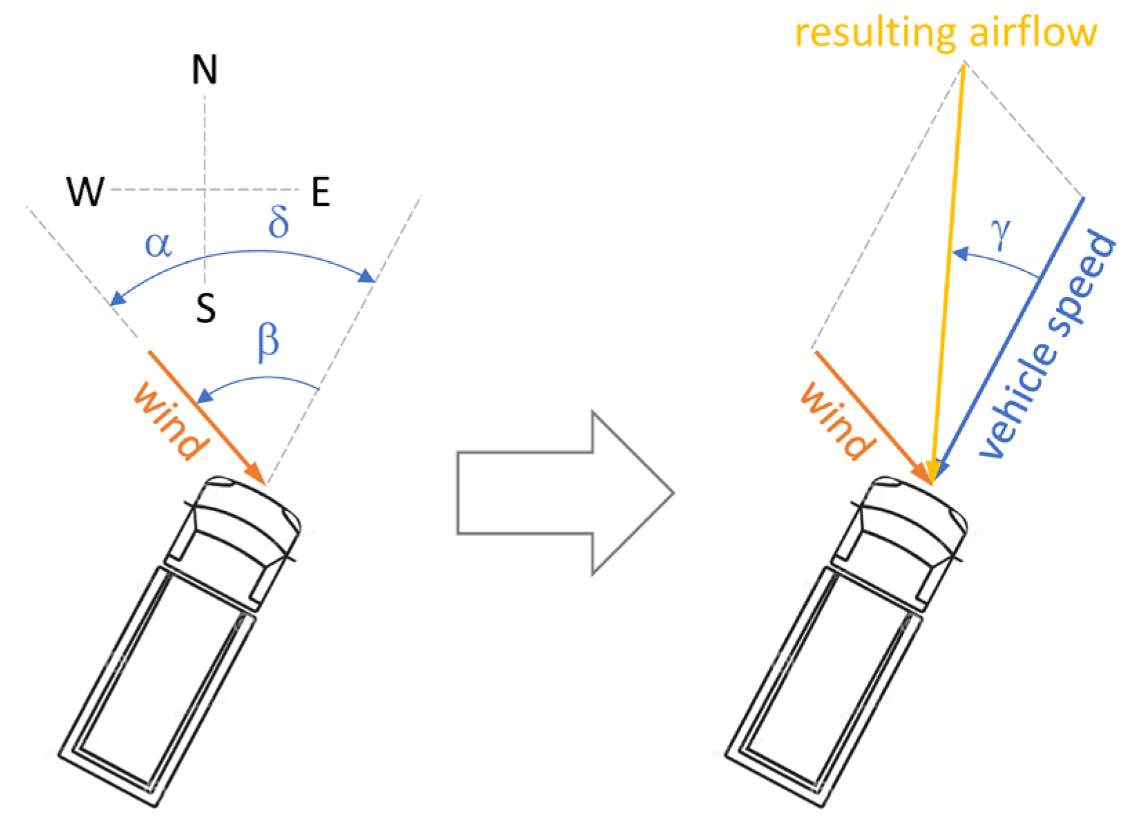
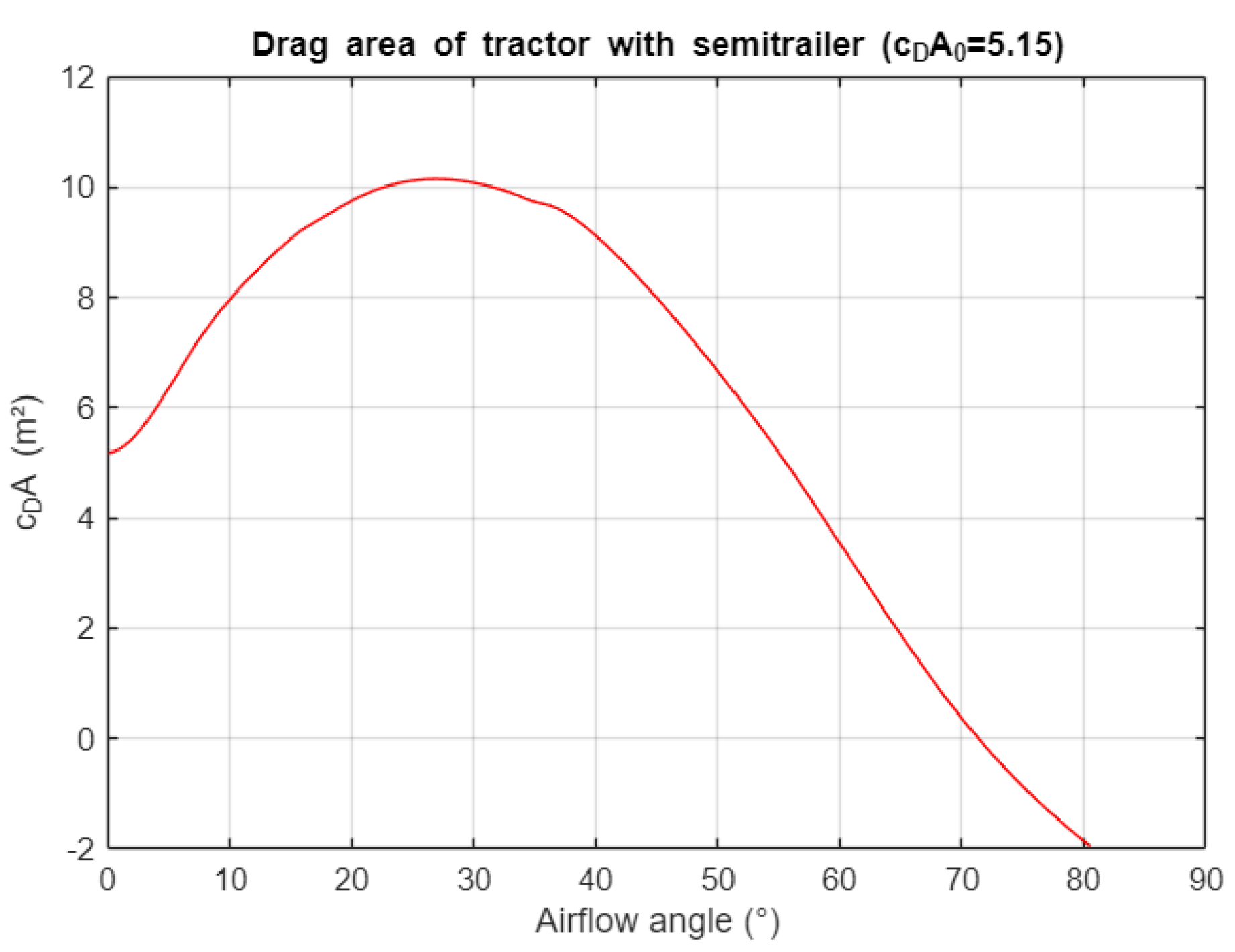
Figure 4.
Airflow angle and speed as a function of wind direction and speed for a vehicle moving at 50 km/h and 90 km/h, respectively.
Figure 4.
Airflow angle and speed as a function of wind direction and speed for a vehicle moving at 50 km/h and 90 km/h, respectively.
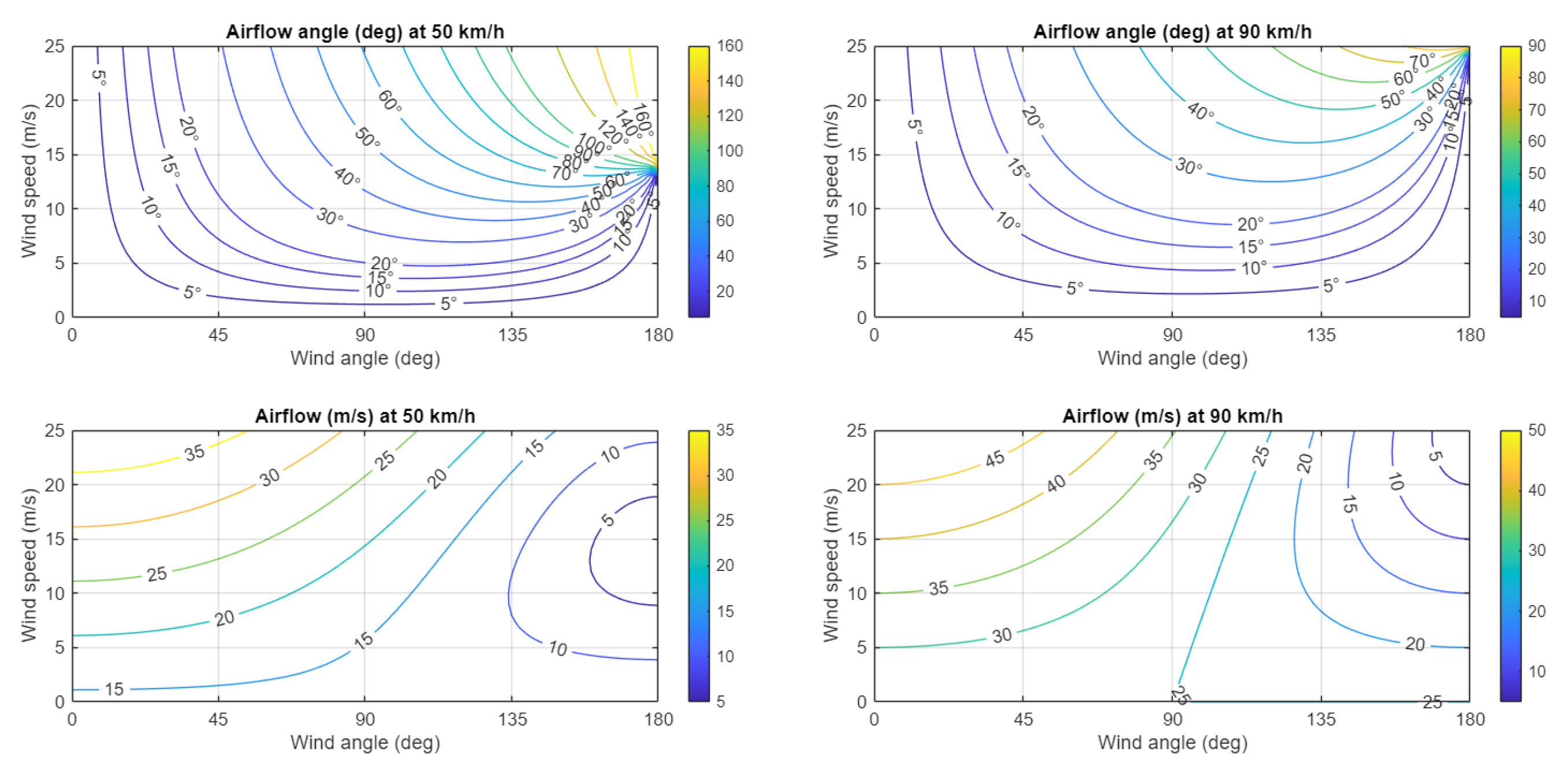
Figure 5.
Generated artificial driving logs.
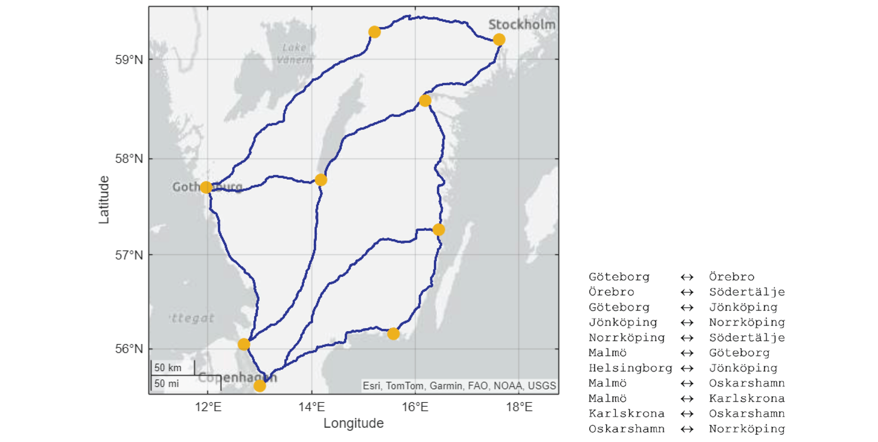
Figure 6.
Comparison of results generated with TrV’s VViS dataset vs. data from the REST API.

Figure 7.
Example of data extraction from TrV stations.
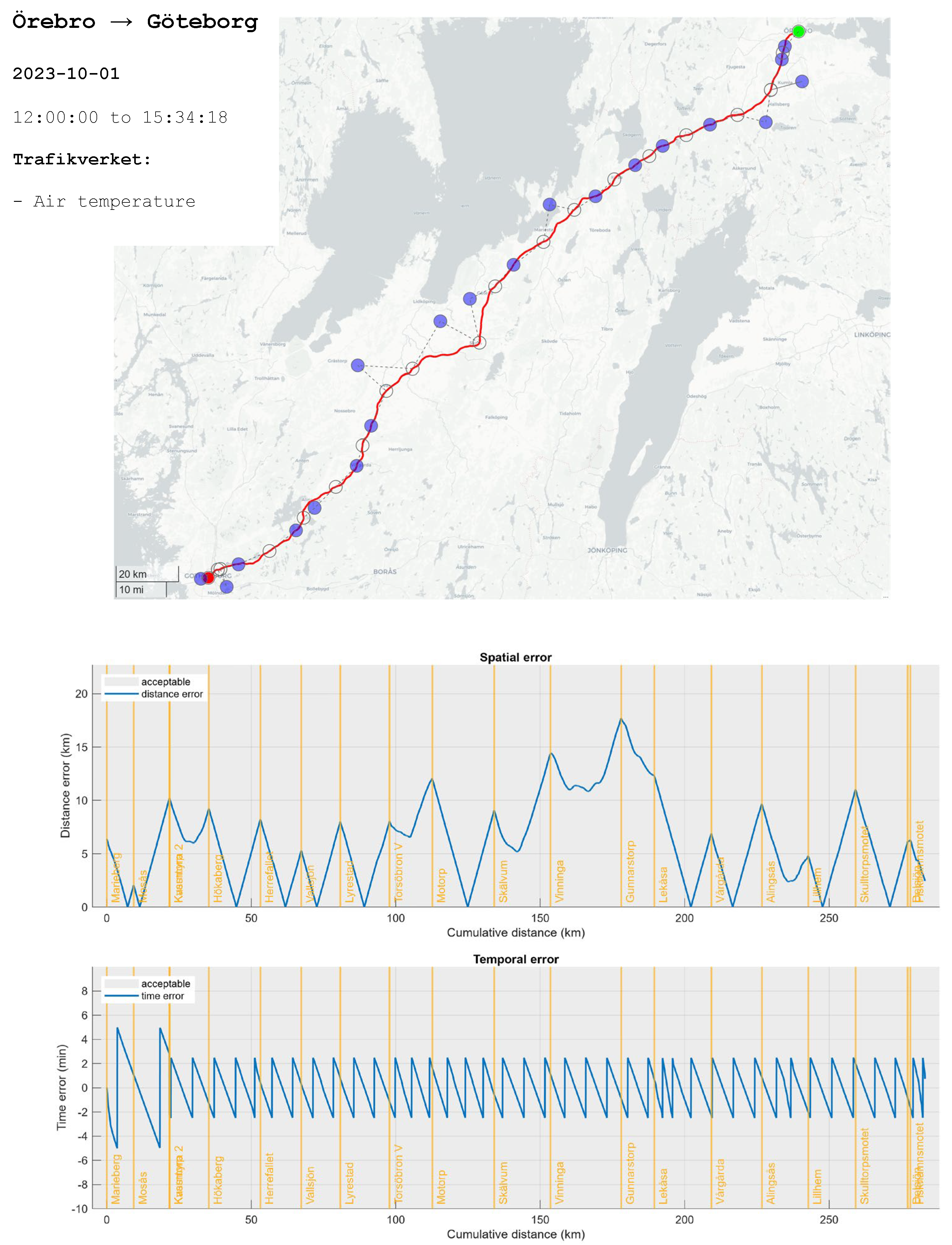
Figure 8.
Example of data extraction from SMHI stations: air pressure.
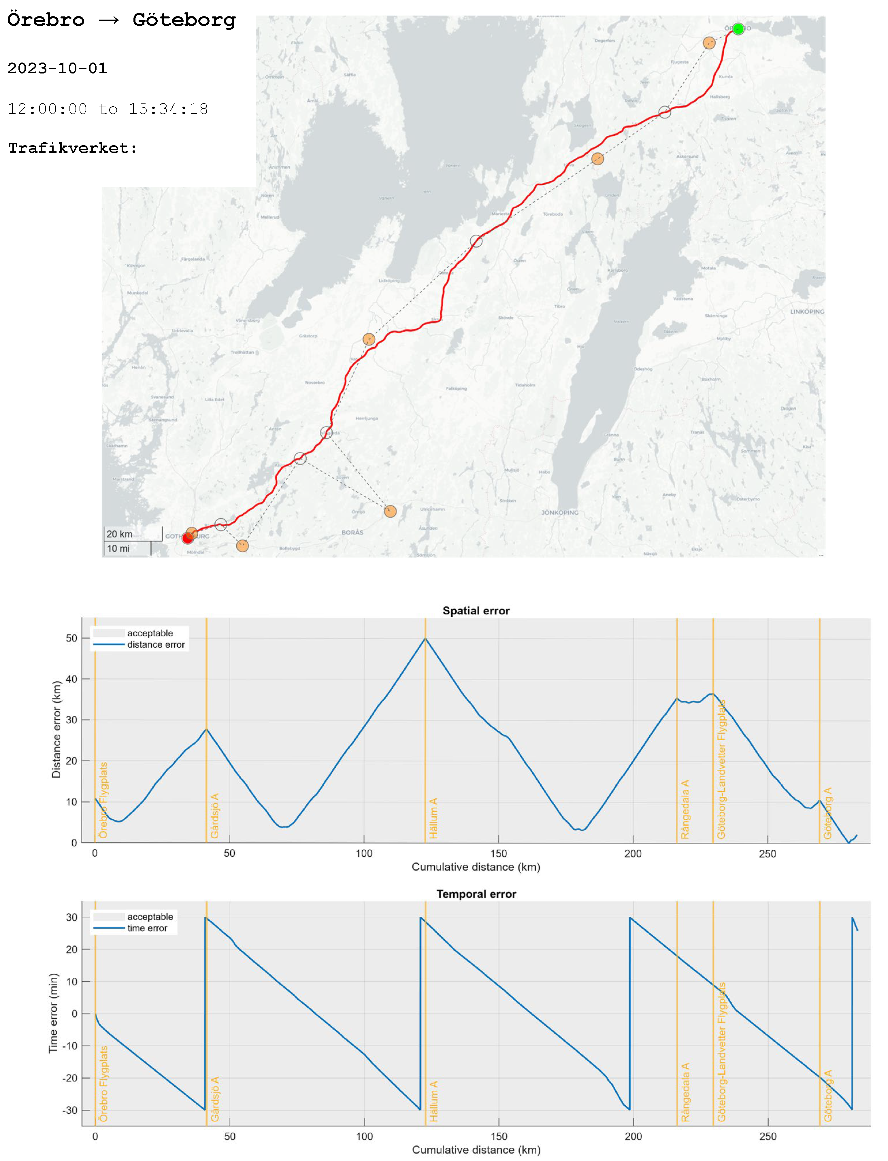
Figure 9.
Example of data extraction from SMHI stations: air humidity.
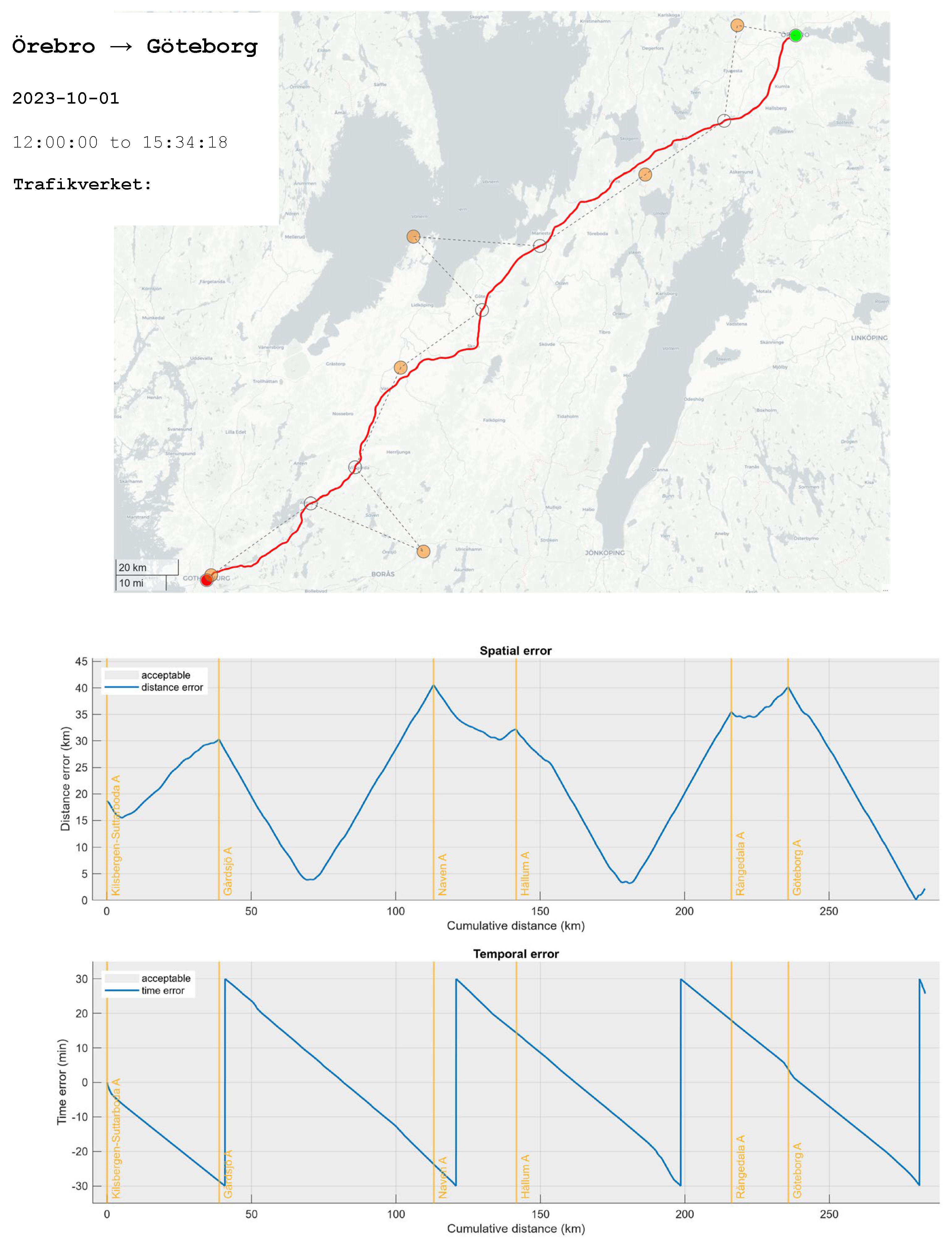
Figure 10.
Airflow, compounded for all routes (all y-axes: probability).
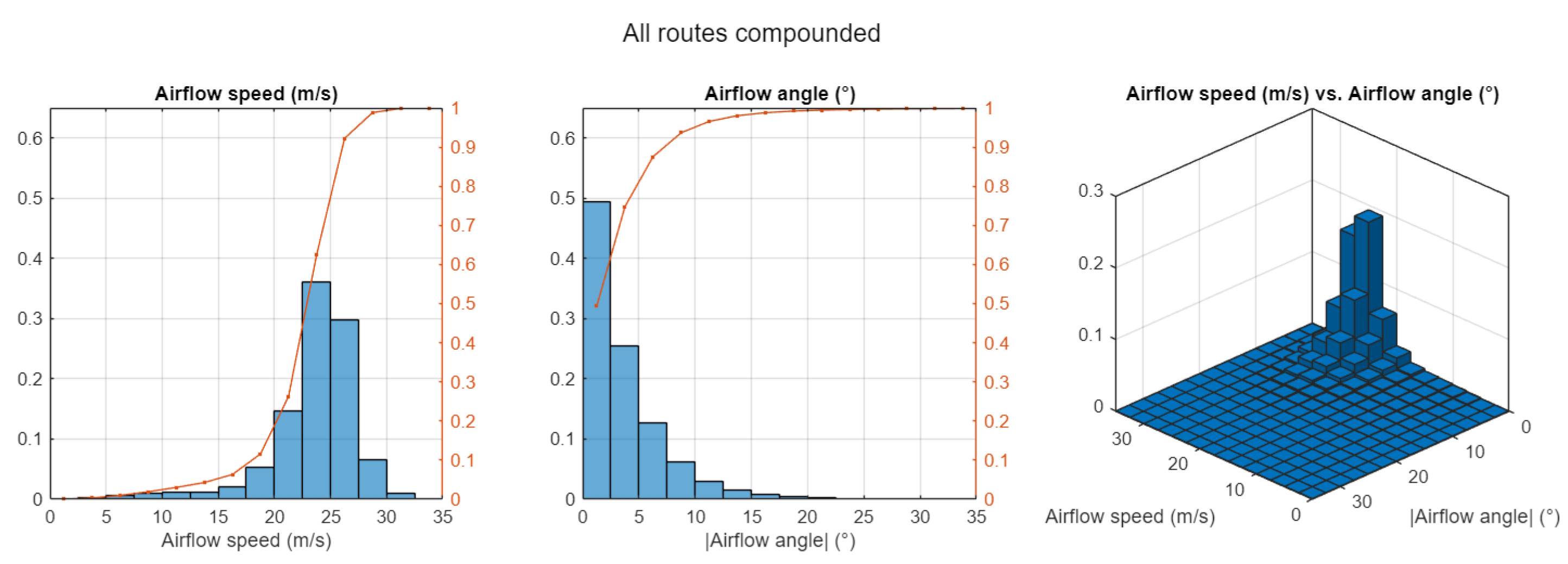
Figure 11.
Specific energy losses due to air resistance, calculated for
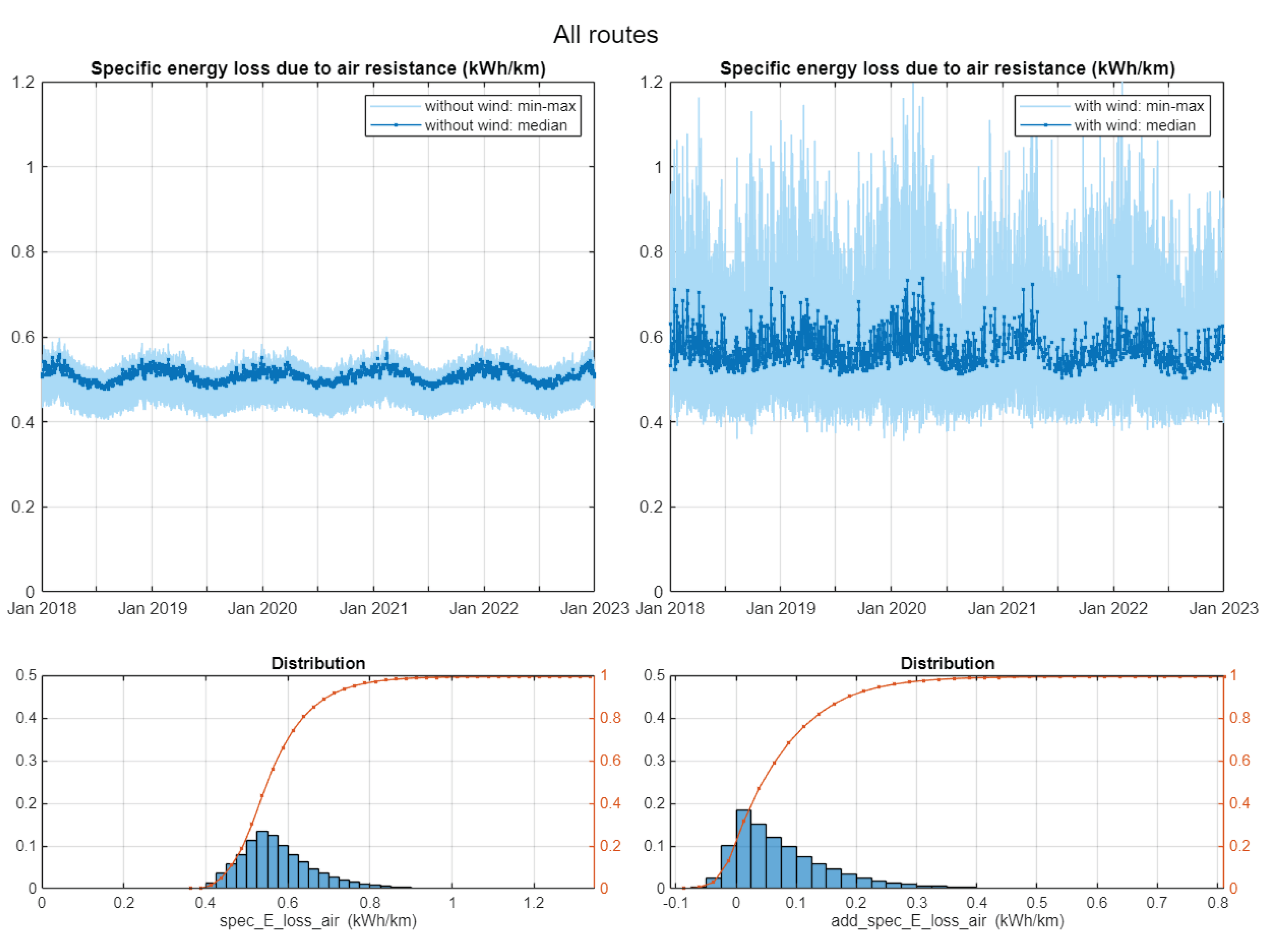

Table 1.
Extracted meteorological data.
| Provider | Parameter |
| SMHI | Air pressure |
| SMHI | Air humidity |
| TrV: VViS | Air temperature |
| TrV: VViS | Wind speed |
| TrV: VViS | Wind direction |
Disclaimer/Publisher’s Note: The statements, opinions and data contained in all publications are solely those of the individual author(s) and contributor(s) and not of MDPI and/or the editor(s). MDPI and/or the editor(s) disclaim responsibility for any injury to people or property resulting from any ideas, methods, instructions or products referred to in the content. |
© 2025 by the authors. Licensee MDPI, Basel, Switzerland. This article is an open access article distributed under the terms and conditions of the Creative Commons Attribution (CC BY) license (http://creativecommons.org/licenses/by/4.0/).
Copyright: This open access article is published under a Creative Commons CC BY 4.0 license, which permit the free download, distribution, and reuse, provided that the author and preprint are cited in any reuse.


