
Submitted:
17 November 2025
Posted:
19 November 2025
You are already at the latest version
Abstract
Einstein derived the expansion of space since the Big Bang and introduced the possible cosmological constant Λ. The expansion of space and the present - day rate H0 of expansion, the Hubble constant, has been discovered by Hubble. Perlmutter et al. discovered the positive value of Λ, and Zeldovich showed that Λ corresponds to the energy density uDE of space. Lamb and Retherford as well as Casimir provided evidence for the idea that uDE might be based on quanta, and Riess et al. provided evidence that H0 is an idealization. In this paper, using the hypothetic deductive method with very founded hypotheses, these two evidences are confirmed in a very founded and precise manner. Thereby, no fit is executed, and no postulate, unfounded hypothesis or assumption are proposed.
Keywords:
relativity
; cosmology
; dark energy
; H0 + tension
; unification
; quantum physics
; gravity
1. Introduction
The properties of space are essential for theories, see e. g. Newton [1], Maxwell [2], Einstein [3], Minkowski [4], Einstein [5], Hilbert [6], Hubble [7], Lamb and Retherford [8], Casimir [9], Zeldovich [10], Perlmutter et al. [11], Smoot [12] and Riess et al. [13]. Thereby, outer space is a relatively ideal form of space in the universe, as outer space is hardly disturbed by molecules or other objects. Hereby, the universe consists of space and of the objects in space.
Moreover, the properties of space are important for applications such as space navigation, see for instance Soffel [14], telecommunication, quantum cryptography or quantum computer networks.
In order to understand space, it is essential to understand that space has a nonzero energy density or . It has essentially been proposed by Einstein [15] in terms of a cosmological constant . And its value has been measured by Perlmutter et al. [11], Riess and others [16], Smoot [12].
Furthermore, space was not given in advance. Instead, space expanded from the Big Bang until today, and space will expand in the future, see Friedmann [17], Wirtz [18], Lemaître [19], Hubble [7], Hobson et al. [20], Workman and others [21], Planck Collaboration [22]. Thereby, the measurable present-day rate of increase of the space exhibits a problem, the - tension: Measurements provide different values of at the 5 confidence level, see Riess and others [13].
This problem is explained here at the level of first principles and a founded and critically reflected scientific method, see sections (Section 1.1, Section 1.1.1).
Firstly, an idealization of space is identified with help of a paradox. The idealization is that in present-day science space as a single entity. With help of a founded derivation, this idealization is overcome: Homogeneous space is a stochastic average of indivisible volume portions.
Secondly, a volume dynamics is derived for these volume portions.
Thirdly, the quantum postulates, gravity, and the Local Formation of Volume (LFV) are derived from this volume dynamics.
Fourthly, based on these founded and derived dynamical processes, the energy density of volume is derived for the case of a homogeneous universe. For that case, this energy density is called . It is in precise accordance with the observed value of the early universe, which was very homogeneous. Moreover, for this homogeneous case, the corresponding value is identified, in precise accordance with observation.
Of course, the universe is heterogeneous. Accordingly, the heterogeneity is analyzed in addition to the homogeneous universe. As a result, the value of the late universe, which is very heterogeneous, is derived. This result is in precise accordance with observation.
These results provide a very convincing evidence for the concept that homogeneous space is a stochastic average of indivisible volume portions. Moreover, these results represent a very clear evidence that the - tension is explained by the gradual evolution of heterogeneity in the universe. These two fundamental insights improve the present-day model of cosmology, the CDM model. Additionally, these findings can be applied to space navigation and exploration, see Carmesin [23,24].
1.1. Hypothetic Deductive Method
In this paper, the results are obtained by the hypothetic deductive method, see Popper [25,26], Niiniluoto, Sintonen and Wolenski [27]. Hereby, the following hypotheses are used:
1.1.1. Used Hypotheses
In this section, the hypotheses are presented that are used in the hypothetic deductive method. Thereby, these hypotheses are very founded. Therefore, the risk of failure is very small.
(1) The space, that can be observed in the whole volume V ranging from Earth to the light horizon, is isotropic and homogeneous at this universal scale. Local heterogeneities are possible, for instance near a mass M, see Schwarzschild [28], Dyson, Eddington and Davidson [29,30]. This has been observed, see Planck Collaboration [22].
(1.1) Moreover, there is natural space that is very homogeneous and isotropic at small scales. For instance, natural space is very homogeneous and isotropic in a void, see Zeldovich, Einasto and Shandarin [31], Contarini et al. [32], and natural space was very homogeneous and isotropic in the early universe, see Planck Collaboration [22].
(1.2) Furthermore, in the heterogeneous universe, natural space can exhibit slight heterogeneity, additionally. For instance, in the heterogeneous universe, Abbott et al. [33] observed the merger of a binary stellar-mass black hole system, and the gravitational waves emitted thereby. These gravitational waves can be interpreted as coherent states that cannot be emitted in a natural homogeneous universe without heterogeneity, as only an appropriate heterogeneity can emit coherent states.
(2) Space has a positive energy density , it is the dark energy density. It is the density of the energy E of the volume V of the space in part (1), divided by this volume:
(3) The energy speed relation of special relativity theory (SRT) holds, see Einstein [3], Hobson et al. [20]: In general, an object with an energy E has a velocity relative to a mass , that is used as a reference. Its absolute value is called speed . In the case of zero speed, , the energy is called rest energy . The energy speed relation of SRT is as follows:
In the case , the relation has the following equivalent form:
Hereby and in the following, the velocity is determined relative to an adequate coordinate system of relativity theory, for details see section (Section 1.1.5).
(4) Each volume or volume portion of space has zero rest energy , and it has zero rest mass .
This is shown in section (Section 1.1.2).
(5) In a process of increase of volume or space, the dark energy density is a nonzero constant, whereby only very small variations might occur. This approximate constancy has been observed for the expansion of space since the Big Bang, see Planck Collaboration [22], Riess et al. [13]. Additionally, that constancy has been proposed by general relativity theory and cosmology, see Einstein [15], Friedmann [17], Lemaître [19], Hobson et al. [20]. Furthermore, the value of is derived here, and the results are additional evidence for this approximate constancy.
The above very founded hypotheses (1) to (5) will be used for deductions in this paper.
1.1.2. Why Volume Has no Rest Mass
In this section, it is shown that volume has zero rest mass .
In the vicinity of a mass M, there occurs additional volume , see section (Section 1.1.4) or Figure 1. If that additional volume would have a rest energy , then there would be an additional rest mass in the vicinity of each mass M. Such an additional rest mass has never been observed, see e. g. Landau and Lifschitz [34], Workman et al. [21], Planck Collaboration [22], Zogg [35]. For instance, if there would be such an additional rest mass , then this would modify the orbits of the GPS satellites, and this would have been observed, but this has not been observed. Consequently, additional volume has no rest mass.
Moreover, the additional volume in the vicinity of a mass is the same type of volume as the usual volume that occurs without any mass. this is confirmed by the observation that only one type of volume has been observed, see e. g. Workman et al. [21], Planck Collaboration [22], Casimir [9], Zeldovich [10], Perlmutter et al. [11]. Therefore, in general, volume has no rest mass.
1.1.3. Mass Causes an Increase of Radial Light Travel Distance
In this section, it is shown that a mass M causes an increase of the radial distance R to M. This increase occurs at each radial difference , see Figure 1.
For instance, in the vicinity of a mass M, an original (at ) radial distance is increased by the square root of the radial element of the metric tensor to a value , see Figure 1,
Hereby, the value can be measured as a light travel distance, see Hobson et al. [20]. Similarly, the original value can be measured with help of two hand leads, the distance is called gravitational parallax distance, see Carmesin [23,36].
As a consequence of general relativity, see Einstein [5], Hilbert [6], Hobson et al. [20], at each radial coordinate (or gravitational parallax distance) R, the radial element of the metric tensor can be expressed with help of the Schwarzschild [28] radius :
These relations are in precise accordance with observation, see e. g. Dyson, Eddington and Davidson [29], Pound and Rebka [30], Will [37].
According to the Hacking [38] criterion of reality, this increase of radial light travel distance is real, as it can be manipulated as follows: The mass M can be increased, and this causes an increase of radial light travel distance , see Eqs. (5 and 6).
Moreover, also the gravitational parallax distance is real, as it can be manipulated as well: For instance, in Figure 1, is the distance between the points A and B. If B moves towards A, then decreases. Next, the corresponding volume is analyzed:
1.1.4. Mass Causes an Increase of Volume
In this section, the following is shown: In the vicinity of a mass M, the increase of the radial length causes an increase of the volume.
Without loss of generality, an portion of volume is used with and .
In the vicinity of a mass M, the radial distance is increased to the respective light travel distance by the factor , while and are not changed by M. Consequently, the volume is increased to the respective volume by the factor , see Eq. (5):
The difference of the volume measured with the gravitational parallax distance and the volume measured with the light travel distance is called additional volume:
The ratio is called relative additional volume :
1.1.5. On the Adequate Coordinate Systems
In the theory of relativity, a time interval of a clock onboard a satellite E and a time interval of a clock onboard a satellite F exhibit the phenomenon of kinematic time dilation. Thereby, relativity theory states: Between two events A and B, a clock in a laboratory coordinate system exhibits a time , a clock onboard the satellite E exhibits a time , and a clock onboard the satellite F exhibits a time as follows:
Hereby, is the speed of the satellite E relative to the laboratory coordinate system, and is the speed of the satellite F relative to the laboratory coordinate system. However, the International Astronomical Union (IAU) realized that relativity theory does not provide information about the choice of an adequate laboratory coordinate system or laboratory frame. Such information about the frame is essential for predicting the times shown by the above clocks, and it is important for space navigation. The IAU called this lack of information the problem of finding an adequate coordinate system (ACS), see Soffel [14].
Thereby, for each point P in the universe, the following has been shown:
(1) An ACS exists.
(2) The ACS has a uniquely determined velocity , relative to an arbitrarily chosen coordinate system .
(3) can be measured, and procedures of measurement are provided.
(4) can be predicted and calculated, and procedures for it are provided.
(5) The equations of time dilation in Eq. (10), as well as the energy speed relation in Eqs. (2 and 3) hold, when the ACS is used. Moreover, the typical results of relativity hold, when the ACS is used.
(6) There exists an absolute zero of the fractional kinematic time difference
whereby the chosen laboratory coordinate system is equal to the ACS.
In this paper, the ACS is used. Therefore, the derived results have clearly defined conditions.
1.2. Observed Energy Density of Volume
In outer space, Perlmutter et al. [11] and Riess et al. [16] discovered the accelerated rate of expansion of the universe. Based on the Friedmann Lemaître equation (FLE), this implies a nonzero energy density of empty space, see e. g. Friedmann [17], Lemaître [19], Hobson et al. [20], Carmesin [40]. It is called density of the cosmological constant or density of the dark energy density [10,15,20,41]. An actual value observed with help of the Cosmic Microwave Background (CMB) is as follows: [22,23,40]
2. Problem of the Hubble Tension
In this section, we summarize a very interesting problem of modern physics. In particular, this problem is a discrepancy of two observed values that should be equal according to the CDM model of present-day physics, see e. g. Hobson et al. [20]. Consequently, this discrepancy falsifies the CDM model. In general, according to the hypothetic deductive method, a solution of such a falsification-problem provides the chance to improve concepts of physics [25,26]. In this paper, we will use the problem in order to develop founded and essential improvements of present-day physics.
Hubble [7] discovered the present-day rate of expansion of space since the Big Bang, the Hubble constant . In general, the Hubble constant is measured by utilizing signals that have been emitted at a time or at a corresponding redshift , see e. g. Hobson et al. [20].
Penzias and Wilson [42] discovered the cosmic microwave background (CMB), a radiation that has been emitted in the early universe, at after the Big Bang. Utilizing that radiation, the Planck Collaboration [22] observed the corresponding value of the Hubble constant:
Hereby, the redshift of emission is . In the measurement, the so-called temperature - temperature correlation, TT, has been used[22] table 2, column 1.
As another example, Riess et al. [13] utilized radiation emitted from supernovae of type Ia in near galaxies and obtained the following observed - value:
Thereby, many galaxies with different redshift values have been observed. Accordingly, the redshift of emission is described by the average of the redshift values of the observed[13] sections 5.1 and 5.2 galaxies, .
Riess et al. [13] observed a discrepancy between the - value based on the CMB and the - value based on near galaxies. Such a discrepancy is called Hubble tension or tension, see e. g. Planck Collaboration [22]. That discrepancy is at the five confidence level. Consequently, that discrepancy can be regarded and named as a scientific result [13]. This result falsifies the CDM model, as this model states that the value of should not depend on the redshift value of observed objects. Based on such a falsification of a model, that model can be interpreted as an idealization, see e. g. Shech [45], Song et al. [46]. Consequently, the idealization of the ΛCDM model is identified:
The Hubble tension falsifies the CDM model. Accordingly, the CDM model is an idealization.
Therefore, the Hubble tension or tension is a founded scientific problem. A fundamental solution of this problem is derived in this paper. Hereby, no fit is executed, no unfounded hypothesis is proposed, and a precise accordance with observation is achieved, and predictions are derived.
Moreover, the value of the Hubble constant of the early universe is a - value of a nearly homogeneous universe, since the early universe was nearly homogeneous [22]. In contrast, is a - value of the late universe, as the observed supernovae occured in the late universe. Additionally, is a value of the heterogenous universe, as the late universe is very heterogeneous [22,47,48].
As the Hubble constant describes the rate of expansion of space since the Big Bang, we analyze the properties of space in more detail. For it, in section (Section 3), we show that the present-day view of space includes a paradox, the so-called space paradox. Moreover, we derive a solution of that space paradox. With it, we will explain and derive the Hubble tension. This solves the problem of the Hubble tension.
3. Space paradox
In general, a paradox provides the chance to develop a deep insight [49]. In this section, we will derive a paradox, and we will use it in order to develop a deep insight.
In the following, the space, that can be observed in the whole volume V ranging from Earth to the light horizon, is considered. For instance, this space has been observed [22].
In physical concepts that are commonly used at the present-day, the space with its volume V is considered as a single entity, see e. g. Newton [1], Maxwell [2], Einstein [5,17], Lemaître [19], Landau and Lifschitz [50], Hobson et al. [20], Planck Collaboration [22].
That space has a positive energy density , see Eq. (1):
As a consequence of SRT, the volume V with its energy E of space, velocity , and speed , obey the energy speed relation, see Eqs. (2 and 3)
As the energy density is nonzero, the energy E is nonzero. Thus, the above relation can be divided by . Therefore, the following form of the energy momentum relation holds:
As a consequence of the zero rest energy of V, see Eq. (4), the right hand side in Eq. (17) is zero. Consequently, the volume V with its energy E has the speed c of light in vacuum.
3.1. The paradox
In physical concepts that are commonly used at the present-day, the volume is considered as a single entity, see e. g. Newton [1], Maxwell [2], Einstein [5], Friedmann [17], Lemaître [19], Landau and Lifschitz [50], Hobson et al. [20], Planck Collaboration [22]. In such a concept of volume, that whole volume would move parallel to some unit direction vector and with the speed of light, , see Eq. (18).
3.2. A solution of the space paradox in natural homogeneous space
(1) The space paradox has five premises: There are four founded premises about space and its volume V, see section (Section 1.1), parts (1) - (4), part (5) is not used here: isotropy, the positive dark energy density, the energy speed relation of SRT (which is correct in the used ACS, see Section 1.1.5), and the zero rest energy . And there is one hardly founded premise (see the beginning of Section 3.1): the concept of space as a single entity. Therefore, space is not a single entity.
As space is not a single object, it must consist of many parts of the volume V. These parts are analyzed next. Thereby, a part of the space with its volume V is called a volume portion (VP).
Hereby, parts of volume with at least one local maximum of volume are analyzed. Thereby, for each part, one such maximum is used in order to localize that part . Such a part is called a localized VP.
Since the energy and volume of space have the speed , the above parts must have the same speed. For instance, each part has its speed
In general, a part of volume is called volume portion.
(2) Next, for the case of a homogeneous universe and space, and for the case of a usual density , The following question is analyzed:
Can such a part with consist of smaller parts ?
Hereby, a usual density is a density below an ultrahigh critical density at which the symmetry of space breaks in a phase transition. This can occur in a phase transition from space to matter in the Higgs [51] mechanism. Moreover, this can take place in a dimensional phase transition [36,40,52,53]).
If such a part with of space would consist of smaller parts , then the following would be implied:
(2.1) Each smaller part would have the speed , as the energy and volume of space have the speed .
(2.2) Consequently, each part would have a velocity , with a direction vector with norm one.
(2.3) As the considered universe is homogeneous (see part (2)), there is no source that could provide a uniform direction of the direction vectors .
(2.4) Hence, the velocity of the considered part with would be an average of the velocities . Thereby, as a consequence of the different direction vectors in part (2.3), the velocity would have an absolute value smaller than c, i. e. . This would contradict the speed in Eq. (19).
(2.5) Therefore, the parts with speeds cannot consist of smaller parts. This is the answer to the question in (2). This implies that the parts with are indivisible. Such a part with its speed is called indivisible volume portion, indivisible VP.
(3) Next, it is shown how the indivisible VPs solve the space paradox:
(3.1) The energy and volume of space have the speed c, and the energy of space obeys , as space consists of indivisible VPs with the speed .
(3.2) Moreover, the velocities of the indivisible VPs have stochastic direction vectors , that are distributed isotropically. Hence, these velocities average to zero.
(3.3) As a consequence, space is isotropic at a universal scale, see Figure 2. In this manner, the space paradox is solved.
Therefore, we obtain the following deep insight, the stochastic property of space:
In a homogeneous and isotropic universe, space is a stochastic average of many indivisible volume portions , each with the speed . Hereby, the velocities of the volume portions average to zero.
(4) Next, the solution is generalized to heterogeneous space: The early universe was very homogeneous and isotropic [22]. The heterogeneity of the mass distribution in the universe increased gradually, and thereby the heterogeneity of space evolved gradually [23,36,48,54,55]. Therefore, the natural heterogeneous space is a slight variation of the natural homogeneous and isotropic space. Details of that variation will be derived in the solution of the Hubble tension below.
3.3. Examples of Parts of Space
In this section, essential parts of natural space with the volume V are analyzed.
(1) Additional volume in the vicinity of a mass M:
In the vicinity of a mass M, there occurs additional volume , see section (Section 1.1.4). It is at rest relative to M. Moreover, in the vicinity of M, the ACS (see Section 1.1.5) [23,24,39]. is nearly at rest at M. Consequently, the speed of the additional volume in the vicinity of a mass is clearly smaller than c, i. e. . Each additional volume with a speed must be a stochastic average of the indivisible VPs with their speeds , as space with its volume V consists of indivisible VPs with their speeds . This is the case for homogeneous and isotropic space and for the case of heterogeneous space which is a slight variation of homogeneous and isotropic space.
Altogether, additional volume that is at rest in the vicinity of a mass M is a stochastic average of indivisible VPs.
(2) Relative additional volume :
In general, a VP is located within an underlying VP . The relative additional volume is the following ratio of the VP and of its underlying VP , see section (Section 1.1.4):
Thereby, the ratio is usually interpreted as a tensor element, whereby the L - direction is the z - direction or the 3 - direction:
In general, a volume portion VP represents a change of an underlying VP , and this change represents a tensor element or tensor. Thereby, typically, the change of each VP has a quadrupolar structure. A dipolar structure is excluded, as volume cannot be negative. Therefore, each change of an underlying VP can be described by a tensor of rank two. It is called change tensor [23,36] . In general, an element of a change tensor is the ratio of the change divided by the underlying length :
Hereby, for each normalized direction vector , the underlying length is the sum of the original length and the change :
In general, indivisible VPs can have the structure of a change tensor as well, see Figure 3.
(3) Gravitational wave:
Without loss of generality, a gravitational wave can be described as follows [50]: It has an angular frequency . At a location, a gravitational wave has one direction of propagation , and two transverse directions and . There are two possible modes. In a first mode, the elongations are and , with , see Figure 3. The second mode is equal to the first mode rotated by 45o around .
The elongations and the velocity of the gravitational wave can be measured with help of a Michelson interferometer. For instance, Abbott et al. [33] measured the amplitude .
In the theory of waves, the above observed gravitational wave is a wave with a coherence length that amounts several wave lengths. Accordingly, a gravitational wave could be interpreted as a coherent state in the framework of quantum physics, if quantum physics is applicable.
3.4. On Quantum Properties of an Indivisible VP
The indivisible VP in homogenous space is very founded. According to this indivisibility, a minimal extension of an indivisible VP is estimated with help of the Heisenberg [56] uncertainty relation of quantum physics:
In general, an indivisible VP can have very different forms, and matter or radiation can be placed in the VP. As an example, and as a very simple model, an indivisible VP is analyzed, that has the form of a ball with a radius , and that contains no radiation or matter.
Consequently, the volume is
Thus, the VP has the following energy:
As the VP has the speed . the energy momentum relation of special relativity theory (SRT) provides the following momentum:
In the rest system of the VP, the momentum is zero, so that the standard deviation alias uncertainty of momentum is estimated by . Similarly, the spatial standard deviation alias uncertainty of the indivisible VP is estimated by
The Heisenberg [56] uncertainty relation for these standard deviations is as follows:
The estimated standard deviations in Eqs. (26 and 27) are inserted into the above uncertainty relation:
This uncertainty relation is solved for the spatial uncertainty :
Altogether, the very particular considered indivisible VP, that does not contain any matter or radiation, has a minimal spatial uncertainty of
3.5. Empirical Evidence for Indivisible Volume Portions
The derivation of indivisible VPs is based on isotropy at small scales. Accordingly, empirical evidence for indivisible VPs is of interest. Such evidence is presented in this section.
3.5.1. Estimated Time Uncertainty of Indivisible Volume Portions
In four-dimensional spacetime, the length of an indivisible VP is estimated by Eq. (30). It is the standard deviation according to the Heisenberg [56] uncertainty relation. In four-dimensional spacetime, the corresponding time uncertainty of an indivisible volume portion is estimated by the ratio of the length and the velocity of light c:
For instance, for the case of an averaging time of one second, , the fractional uncertainty is estimated as follows
3.5.2. Time Uncertainty of an Atomic Clock Using Gas
Many atomic clocks use gas atoms [57,58]. As these atoms move in natural space, and as an atom is very small compared to the estimated size of an indivisible VP, the clock’s uncertainty is larger or equal to the uncertainty of an indivisible VP in homogeneous natural space, in general. Similarly, if an object moves within a ship, then the object’s uncertainty is larger or equal to the ship’s uncertainty, in general.
For the case of natural space consisting of indivisible VPs, the uncertainty of space is estimated by in Eq. (32). Therefore, for the case of averaging of one second,
In general, the uncertainty of a clock can be reduced by averaging during a time . Thereby, according to statistics, and according to observation, the uncertainty decreases by the factor [57,59]. Empirical data show the following [57]: Atomic clocks that use gas atoms, that are not confined to any particular location or trajectory, and that are averaged at most one second, , exhibit time uncertainties larger than the estimated uncertainty of indivisible VPs in Eq. (32). This provides evidence for the existence of indivisible VPs. Moreover, a control experiment is available:
3.5.3. Time Uncertainty of an Atomic Lattice Clock
In an atomic lattice clock, the used atoms are confined to the potential minima of a standing wave of laser light. Hereby, the standing wave, and the device that generates that wave, are large compared to the estimated size of an indivisible VP. As a consequence, these atoms do not move freely in an indivisible VP of homogeneous natural space, but in artificially generated potential minima. Therefore, the atomic lattice clock’s uncertainty can be smaller than the estimated uncertainty of indivisble VPs in Eq. (32). In fact, measurements show that this is clearly the case. There is even a local maximum of the uncertainty as a function of the time of averaging [60]:
This control experiment provides evidence for the following: The independence of the uncertainty of natural space and of indivisible VPs can provide a very small uncertainty of an atomic lattice clock.
4. On the Dynamics of Volume Portions
In this section, a very valuable and insightful description of VPs is developed. With it, a very general differential equation (DEQ) of the dynamics of VPs is derived.
Here and in the following, mathematically, a VP could be arbitrarily small. Physically, the Heisenberg [56] uncertainty relation limits the standard deviation of a VP from below. A particular example is analyzed in section (Section 3.4).
4.1. Additional Volume
In this section, the increase of the volume of a VP is analyzed. For it, the difference of the increased volume and the original volume of the VP is used:
Hereby and in the following, a light travel distance is larger or equal to the corresponding gravitational parallax distance , i. e. , so the particular case without curvature is included. The above difference is called additional volume, see section (Section 1.1.4).
Similarly as in section (Section 1.1.3), according to the Hacking [38] criterion, the enlarged volume and the additional volume are real, as they can be manipulated. In contrast, the original volume is an idealization corresponding to the idealization of flat space:
Each VP has a real additional volume and a real enlarged volume , according to the Hacking [38] criterion.
In order to derive general laws of physics, this difference is normalized in the next section:
4.2. Relative Additional Volume
In general, in order to derive general laws of physics, it is valuable to use intensive quantities rather than extensive quantities [61]. In the present case of a VP, it is useful to utilize the ratio of its real additional volume and its real enlarged volume . Such ratios are formed and analyzed in detail in this section:
This is an example for the fact that curvature can be described by the metric tensor or by the relative additional volume. Moreover, the relative additional volume of a VP is real, as it is a ratio of real quantities of that VP:
Each VP has a real relative additional volume.
Furthermore, the description with the additional volume is compatible with the volume portions that become necessary for the solution of the space paradox. In contrast, the metric tensor does not include the concept of volume portions, and it does not provide the dynamics of the volume portions. As a consequence, the description with the volume portions provides the additional possibility to derive the dynamics of volume portions. Of course, the metric tensor provides the description of time dilation directly. In the case of volume portions, the Schwarzschild [28] metric is used. Thereby, the tensor element of the time is utilized. With it, an interval of coordinate time is transformed to an interval of own time [20]. With help of the volume portions, the dynamics of volume portions is derived next:
4.3. Dynamics of Volume Portions
In this section, the dynamics of an arbitrary VP is described by its relative additional volume. The result is achieved with help of calculus or standard analysis only. As a consequence, the dynamics of VPs derived here is very general.
Firstly, the applicability of calculus or standard analysis is investigated:
Calculus or analysis are a mathematical tool, such as algebra and stochastics. Thereby, calculus or analysis do not include a prejudice about the continuity of space and time. The reason is that in the present investigation, space is a stochastic average of VPs. Hereby, VPs will be characterized by eigenvalues with a spectrum of eigenvalues. This spectrum can turn out to be discrete, continuous or partially discrete and partially continuous. As calculus or analysis are used in this study, these fields of mathematics do not necessarily include a prejudice about the discreteness or continuity of space.
In contrast, an exclusion of calculus and analysis would include a prejudice about the discreteness or continuity of space.
In fact, the space paradox and the implied structure of space as a stochastic average of VPs does already deduce an essential degree of discreteness of space. And it is important to investigate the amount of discreteness and continuity of these VPs in the following.
Moreover, in this paper, the physical reality of the used and deduced concepts is permanently tested with help of the Hacking [38] criterion.
Secondly, the differential equation, DEQ, of VPs is derived:
Each localized VP (see Section 3.2, part (1)) has a local maximum of its relative additional volume . It is a function of its three-dimensional position vector and of the time . It is illustrated in Figure 4, whereby the three-dimensional position vector is summarized by a position L. Altogether, a localized VP can be described by a function with a local maximum. If there should be several local maxima or a set of local maxima, then one local maximum can be chosen as a convention.
As a fact of calculus or of analysis, at the local maximum, the change of is zero. Thus, the total derivative is zero:
That derivative is evaluated with help of partial derivatives:
The VP moves parallel to a corresponding direction unit vector of its velocity . Therefore, during a time , the vector changes by the amount = . With it, the total derivative in Eq. (40) is
The above Eq. is divided by . Moreover, the Eq. is solved for :
This is the differential equation, DEQ, of VPs or of volume dynamics (VD). A Lorentz invariant form of the DEQ is achieved as follows. The square is applied to Eq. (42), and the right hand side is subtracted,
For the following reasons, the derived dynamics is very founded and insightful: The derived DEQ of VD describes the dynamics of a VP with at least one local maximum. The derivation uses no postulate or unfounded hypothesis. In contrast, general relativity uses postulates such as the Einstein Hilbert action or the Einstein field equation [5,6]. Similarly, quantum physics uses ’guessed’ postulates [62,63,64]. Also gravity uses ’guessed’ postulates or restrictions. Examples are the restriction to physics without quanta in general relativity [5], and in Newton’s gravity [1]. Another example is the graviton hypothesis. Thereby, gravity uses hypothetic quanta [65].
Indeed, we will show later that the DEQ of VD implies gravity and curvature of space and time. Moreover, we will show that the DEQ of VD implies the postulates of quantum physics. In particular, based on the VD, we derive the Schrödinger equation in the next section.
5. Derivation of the Schrödinger Equation
In this section, we show that each VP fulfills a generalized Schrödinger equation (GSEQ), which implies the usual Schrödinger equation (SEQ), which holds for the special case of a non-relativistic mass M.
5.1. The Volume Dynamics Implies the GSEQ
In this section it is shown, that VPs with their VD imply the GSEQ.
(1) In a first investigation, the geometry of relative additional volume is analyzed:
For each VP, the DEQ (42) of VD is fulfilled. Thereby, the VP moves in the direction of its velocity, see Figure 4.
In general, a relative additional volume with an increase with the normalized direction vector and with a propagation of indivisible VPs in the same direction, and with an underlying length , is called unidirectional relative additional volume , see Eqs. (21, 22 and 23). More information about such tensors can be found in the literature [23,36,50,66,67].
(2) Next, each VP is described by the DEQ of VD. In that DEQ, is inserted. Additionally, the time derivative is applied, so that the relative additional volume becomes , which is usually expressed by . As a consequence, the DEQ of VD implies the following DEQ:
(3) Next, as an equivalence transformation of the above DEQ, the factor is multiplied. This multiplication is also physically equivalent, as the system of units can be chosen freely. And the factor ℏ is one in natural units [68]. Consequently, the DEQ of VD implies the following DEQ:
Moreover, for the case of an indivisible VP, this indivisibility corresponds to the quantum property with its universal unit of quantization, the Planck [69] constant h or its reduced version .
Accordingly, the correspondence principle is applicable [68]. Consequently, the rectangular bracket is identified with the momentum operator[67] chapter 9:
In this DEQ, represents a rate. That rate is normalized by a factor . In physics, has the dimension time and the unit second. Consequently, the normalized rate is dimensionless and has the unit one. It will be shown that the normalized rate has the role of a wave function in the above DEQ. Accordingly, the normalized rate is called wave function . Of course, this can be regarded as an abbreviation, if desired. As a consequence, the DEQ of VD implies the following DEQ:
The product of the momentum operator and the direction vector of propagation, , is the operator of the absolute value of the momentum :
In the present case of a VP that propagates with the speed c, special relativity implies that the product of c and the momentum p is the energy E. Consequently, according to the correspondence principle [68], pages 673-674, the product of c and the momentum operator is the energy operator:
This Eq. has the form of a Schrödinger equation, SEQ. However, the SEQ holds for non-relativistic objects. In contrast, this DEQ holds for relativistic objects too, and it implies the SEQ for non-relativistic objects, see next section (Section 5.2). Thus, this DEQ is the GSEQ. Moreover, is real, as it is the derivative of the real . As a consequence, the wave function is real, as it is the normalized form of the real .
5.2. The Volume Dynamics Implies the SEQ
In this section it is shown, that VPs with their VD imply the SEQ.
For each localizable quantum object at , the following is implied:
(1) For the case of ultrafast objects, with [21] an energy eigenvalue is obtained by the following linear approximation of the energy momentum relation with respect to the small ratio :
Hereby, marks the first order approximation for small . The corresponding linear approximation of the GSEQ is obtained by replacing the eigenvalue p by its operator :
(2) For the case of slow objects, with , the following holds:
(2a) An energy eigenvalue of the energy is obtained by the following linear approximation of the energy momentum relation with respect to the small ratio :
(2b) The corresponding linear approximation of the GSEQ is obtained by replacing the eigenvalue p by its operator .
Hereby, the wave function includes the rest energy . Accordingly, the wave function is named . In general, the following squares are equal:
(2c) The wave function is factorized:
The left hand side of Eq. (54) is evaluated with the product rule:
(2d) In the above DEQ, is subtracted. The resulting DEQ is divided by . As a consequence, the SEQ proposed or postulated by Schrödinger [72] is derived from the VD:
Additionally, can include a potential energy:
5.3. Interpretation of VPs and Masses
In this section, the relation between VPs and masses is elaborated on the basis of the above dynamics of the VD, the GSEQ and the SEQ, and of the Higgs [51] mechanism:
In physics [9,68,76], empty space is called vacuum, and its energy density is the density of dark energy [11,77]. In the above phase transition, the vacuum transforms to a mass.
As shown by the space paradox, the vacuum is a stochastic average of indivisible VPs. As a consequence, the above phase transition transforms indivisible volume portions to a mass.
In a typical phase transition, objects change from one phase to another phase. Thereby, these objects are described by the same fundamental dynamics in the first phase, in the second phase and during the transition. An example is the phase transition of condensation [78,79].
In the present case, such a fundamental dynamics that holds in the first phase, in the second phase and during the transition has been derived. It is the DEQ of VD. It holds for VPs in the first phase, and it implies the SEQ that holds for the masses in the second phase. A description of the phase transition in the framework of the VPs is elaborated in Carmesin [75].
Of course, the question remains how a mass can emit its wave function. This will be derived in the next section: In part (Section 6), it is shown that the VPs provide gravity as well as the local curvature of space and time as a byproduct. It has already been shown that a mass causes additional volume and VPs, see sections (Section 1.1.3 and Section 4.1). In section (Section 7), the process of local formation of volume (LFV) and of VPs is described, and a corresponding DEQ of the LFV is derived. These VPs formed by a mass M represent the wave function of that mass. In part (Section 10), it is shown for the case of the homogeneous universe, that this DEQ of LFV provides the emergence of the space of the universe and of the energy density of that space in a homogeneous universe. More generally, in a heterogeneous universe, the energy density of space is , and the difference of and increases gradually with the heterogeneity of the universe, and this difference remained relatively small during the time from the Big Bang until today.
Both results are in precise accordance with observation. Therefore, these results provide a clear evidence for the present theory of VPs.
6. Gravity and Curvature
In the vicinity of a mass M, there occurs a curvature of space, as well as an exact gravitational potential and field, see Figure 1. Next it is shown how these phenomena are implied by the DEQ of VD:
6.1. Potential and Field
In this section, an exact generalized potential and generalized field are derived from the volume portions.
6.1.1. Generalized Potential and Field
In the vicinity of a mass M, see Figure 5, the unidirectional radial relative additional volume exhibits the following properties. Hereby, spherical polar coordinates with M at the origin, at and at in Figure 5 are used:
(1) For each indivisible VP , the relative additional volume propagates according to the DEQ of VD.
(1.1) That DEQ is multiplied by c:
(1.2) At an event , including the set of its surrounding events in a time interval and in a ball , with in the vicinity of the mass, the sum of the relative additional volume of all indivisible VPs is applied:
(1.3) The bracket in the above DEQ has the form of a generalized potential
Hereby, the potential is generalized, as it describes volume portions, since is the relative additional volume of an indivisible VP.
(1.4) The negative gradient of that generalized potential is the generalized field , see Figure 5:
The potential and field in the above equation are generalized to the respective quantities for one indivisible VP . Thereby, the potential is
and the field is as follows:
These relations are results of the VD. Formally, these results can be obtained by an application of the above average with one indivisible VP only.
For comparison, expectation values of the field have been derived from the VD as follows: Firstly, a quantum field theory has been derived from the VD. Secondly, the expectation value of a field has been derived from the quantum field theory [23,67].
(2) For these indivisible VPs, and for each event , that rate gravity relation can be expressed with help of the following rate gravity scalar:
(3) For each underlying volume , and for each event , with a gravitational parallax distance R from M, the generalized field is proportional to :
This result is derived as follows:
(3.1) Eq. (64) is multiplied by . Hence, the field is as follows:
(3.2) Integration with respect to from zero to a time yields:
The time is chosen so small that the integral in the above Eq. is approximated by . Thus, the field is as follows:
(3.3) The definition is used. The energy density of volume is nonzero, as it is approximately the same as , which is nonzero [11,12,16]. Therefore, the indivisible VP is proportional to the corresponding energy . The latter is proportional to the momentum , as each VP propagates with the speed c, that is: .
(3.4) The underlying volume of a shell with center M is considered. It is as follows: . Thus, the field is as follows:
Hereby, the thickness of each shell is chosen constant, so that it does not dependent on R. Thence, the first fraction is constant. The 2nd fraction is the momentum current flowing through each shell. It is constant, as no shell causes any momentum. Consequently, . q. e. d.
A version of the corresponding result for a dimension is shown in Carmesin[67] THM 9.
(4) As M is the source of the field , that field is proportional to M: .
Thus, there is a universal constant of proportionality:
In general, the value of a universal constant, such as , must be obtained from observation. Accordingly, is obtained in the next section. Additionally, the curvature of space is analyzed:
6.1.2. Spin, Statistics and the Additive Structure of VPs, Potentials and Fields
In general, a VP has the tensor property of a quadrupolar structure, see section (Section 3). Consequently, it is represented by a tensor of rank two.
Therefore, at the level of quantum physics, an indivisible VP has an integer valued spin, see Landau and Lifschitz [81], §58, Carmesin [82]:
As a consequence, at the level of quantum physics, an indivisible VP is a boson, see Landau and Lifschitz [81], §64, Carmesin [82]. Consequently, at the level of quantum physics, an indivisible VP obeys the Bose [83] statistics, alias Bose - Einstein statistics, see Landau and Lifschitz [81], §64, Sakurai and Napolitano [63], section 7.2.
The Bose - Einstein statistics implies that several bosons can exist at the same place. Consequently, the additional volumes caused by different masses can exist simultaneously at each point P in the universe, and these add up at P. This, in turn, implies that the potential at P is the sum of these additional volumes multiplied by . This founds Eq. (62) at the level of quantum physics. As a consequence of this potential, the generalized field has the same additive structure.
6.2. Curvature in the Vicinity of a Mass
The DEQ of VD provides the curvature in the vicinity of a mass M as follows:
(1) For the case of a shell with the center M and with the gravitational parallax radius R, the relative additional volume is as follows:
The fraction is identified with the root of the radial tensor element of the metric tensor. It occurs in the vicinity of a mass M.
More generally, at each R, or at each event with , the curvature can be generalized for the case of a single indivisible VP , with the relative additional volume , as follows:
(2) A DEQ for the position factor is derived: For it, is applied to Eq. (79). This implies:
The potential is solved for , and this is inserted into Eq. (82):
The gradient is applied:
The field is identified:
The field and the direction vector are antiparallel. Consequently, the field is as follows:
The field as a function of the mass in Eq. (76) is used:
(3) The DEQ for the position factor is solved:
Integration by parts yields:
The integral is evaluated with a constant K of integration:
That result is solved for the position factor:
In the limit , there is no curvature. Consequently, . As a consequence, . Therefore, the solution of the DEQ provides the position factor as follows:
(4) The position factor in Eq. (91) is compared with observation. For it, the position factor is replaced by the inverse root of the radial tensor element (see Eq. 80):
Moreover, observation shows that this inverse root of the radial tensor element is as follows [20,84]:
Hereby, we use the definition of the Schwarzschild radius . The comparison of the two relations for the tensor element in Eqs. (92 and 93) shows that the generalized universal constant is the same as Newton’s constant of gravitation G. Thus, the generalized field is identified with the exact gravitational field and the generalized potential is identified with the exact gravitational potential. These identified potential and field are exact, as they are derived without any approximation, and as they provide the correct curvature. This exact gravitation, derived here exactly, differs from Newton’s law of gravitation, which is an approximation.
In the vicinity of a mass, the indivisible VPs cause a generalized potential, a generalized field, the gravitational field and the curvature of space and time. The respective Eqs. are derived.
6.3. Discussion of Gravity and Curvature
In the vicinity of a mass M, the VD provides the relative additional volume as a function of r. That provides the exact gravitational potential . That exact gravitational potential provides the exact gravitational field . In the following, these valuable and insightful properties are analyzed and interpreted:
6.3.1. Transmission of the Potential and Field
The indivisible VPs with their relative additional volume provide a net outward propagation. Thereby, these indivisible VPs transmit a nonzero momentum, as the energy density is positive. As a consequence, these indivisible VPs transmit the gravitational interaction. This confirms the idea of the graviton hypothesis proposed by Blokhintsev and Galperin [65]. Moreover, these indivisible VPs explicate the mechanism of the transmission of gravity.
6.3.2. On the Exactness of the Potential and Field
The generalized potential and field derived here are exact. In contrast, the gravitational potential is only an approximation in Newton’s theory. For instance, correction terms depending on the gravitational parallax distance R and on the velocity have been elaborated in Post-Newtonian approximations [85,86], Eq. (2.49). Accordingly, the following question arises: How is the exactness achieved here?
Essentially, this is achieved here by the application of especially useful distance measures and coordinates systems:
Firstly, for each point P in the universe, there is an adequate coordinate system (ACS), so that an object at rest in the ACS has the absolute zero of velocity, see section (Section 1.1.5) or Carmesin [23,24,39]. This ACS is used here. As a consequence, the velocity-terms in Post-Newtonian approximation are zero.
Secondly, two measurable distance measures are used, see Figure 1: the light travel distance [87], and the gravitational parallax distance [23,36,40], it can also be measured as a circumferential distance [88,89], section 2.6.
Hereby, according to the Hacking [38] criterion, the light travel distance to a field generating mass M is real, as an increase of M can change that distance . In contrast, the gravitational parallax distance to a field generating mass M is idealized, as it represents the limit M to zero of the light travel distance:
This is a typical idealization based on a limit [46]. Though the gravitational parallax distance is idealized and not real, that distance can be measured, and that distance provides the law, see Figure 5.
Thirdly, the exact potential and field are determined as follows: For the case of a point P, the idealized gravitational parallax distance from P to the field generating mass M is measured or determined by other means. With it, the potential and the field are determined as a function of , by using the respective equations in this section and paper. The result is exact, as no approximation has been used in the derivation of these equations.
In contrast, in Newton’s theory, the flatness of space has been introduced as a postulate. Accordingly, a user might use that postulate and the light travel distance , and the equations for potentials and fields in Newton’s mechanics. In such a postulate based determination of the potential or field, the result is an approximation only.
6.3.3. Advantage of the Exact Potential and Field
Altogether, the indivisible VPs cause the transmission of gravity, the exact gravitational potential, the exact gravitational field and the exact curvature of space, in an indivisible and impartible manner. Thereby, by using the adequate coordinate system and the measurable idealized gravitational parallax distance, relatively short, highly structured, and clarifying equations can be used. Moreover, the results are parts of the unification of relativity, gravity and quanta. This unification uses the relative difference , which is based on both distance measures: the real and the idealized .
7. Local Formation of Volume in Nature
In this section, the dynamics of the local formation of volume (LFV) is derived.
In the vicinity of a mass M, additional volume propagates outwards in a radial direction. Thereby, the amount of additional volume increases. Consequently, there occurs locally formed volume, LFV, or in the radial direction r. Hereby and in the following, an underlined variable marks the formed volume or the process of formation of volume. Such LFV can be caused by the mass M.
More precisely, that LFV occurs at each location. At each location, there is a gradient of the relative additional volume , or of the potential , or there is a gravitational field . As a consequence, more generally, locally, the LFV is caused by a local gravitational field. In this section, the relation between the LFV and its cause is analyzed: the field or .
7.1. Definition of Locally Formed Volume
If additional volume forms in a volume and in a direction during a time , then this process can be described by the following normalized rate of unidirectional LFV:
That LFV is described by a general law, which is derived in the next section:
7.2. Law of Locally Formed Volume
In this section, the mechanism of the local formation of volume is explained and formulated. This law of the local formation of volume is derived in section (Section 7.3).
In the vicinity of a mass M or an effective mass , and at a based distance R from M or , the following holds for the normalized rate:
(1) In the far distance approximation, FDA, the ratio is relatively small compared to 1. Thereby, at first order in that ratio , the normalized rate is as follows:
Hereby, is the component parallel to of the generalized field. is the cause of the rate of LFV . More generally, each field in a direction causes a unidirectional normalized rate in that direction. Moreover, this field is equal to the exact gravitational field , see section (Section 6):
(2) As a consequence, the non-diagonal components do not provide additional volume.
(3) The exact value of the rate is:
(4) More generally, is a function that has to be determined. The definition yields = . The substitution = = yields = . The substitution = = yields = . Using , and = yields: = = . Evaluation of the derivative yields = = - . = and imly
(5) Eq. (99) can be solved numerically and provides the metric in a rotation symmetric system:
7.3. Derivation of the Law of LFV
In this section, the mechanism and the law of local formation of volume are derived.
Part (1): At each radial coordinate R, a shell with center at M, and with thickness represents the analyzed volume . Thereby, the additional volume is in a shell with radius R, thickness , and volume . Similarly, the LFV is in a shell with radius R, thickness , and volume .
The LFV is analyzed at leading order in the increment . This is exact, as the increment can be made as small as desired. If the additional volume increases as a function of R, then there occurs formed volume , whereby the direction r is equal to the radial direction.
In general, the observable additional volume in a shell with center N, with radius R, and with thickness is a function of R. Consequently, the LFV is the change of as a function of R. Therefore, the change of volume in a shell with thickness is equal to the derivative of the observable additional volume multiplied by that thickness :
Thereby, is as follows:
In the far distance approximation, FDA, in leading order in , is as follows:
With it, the derivative in Eq. (101) is as follows:
With it, the change in Eq. (101) is as follows:
With it, and with , and with , the normalized rate of unidirectional LFV in Eq. (95) is as follows:
With it, and with , the normalized rate of unidirectional LFV in Eq. (106) is as follows:
The above fraction is the absolute value of the field. Thereby, the field is antiparallel to the radial unit vector :
Application of the square yields Eq. (97):
In the case of an effective mass, there is no rotational invariance with respect to , in general. In that case, the proof is performed for each angular direction separately[89] chapter 9. Moreover, each field parallel to a direction causes a unidirectional rate , according to Eq. (97).
Part (3): We analyze the rate in Eq.(95):
The change is the change of
As the time of propagation is incremental, and since a field in the radial direction causes changes in the radial direction only, we can express the difference at linear order in :
Next, L is substituted by R:
Next, is used, as well as :
The derivative is evaluated:
8. Energy Density of the Gravitational Field
In this section, the energy density of a gravitational field is introduced and derived.
8.1. Measurement of the energy density of the field
The energy density of the field can be measured as follows: A rest mass is distributed uniformly in a shell with a radius R and a small thickness , see Figure 6. That mass is lifted by a radial difference . Thereby, the required energy is measured. This energy is located in the field within the shell with center M, thickness and radius R, see Figure 6. That shell has the volume
Consequently, the absolute value of the measured energy density is as follows:
The positive required energy compensates the energy of the field in the shell, as the field in the shell with volume is eliminated in the process of lifting the mass. Consequently, the sign of the field is negative:
Alternatively, this measured energy can be calculated:
8.2. Derivation of the Energy Density of the Field
The required energy can be calculated [67]:
The measured energy density in Eq. (119) can be calculated by inserting Eqs. (120 and 117) into Eq. (119):
For comparison, [91] derived the same formula for the energy density
Peters [91] derived this result in a Newtonian approximation.
In contrast, the exact energy density is derived here. This is achieved with help of the exact field, since no approximation is used here. This exactness is achieved here with help of the distinction between the two distance measures: the gravitational parallax distance and the corresponding light travel distance .
8.3. Compensation of the Negative Field
The sum in the above Eq. is identified with the summed relative additional volume of the indivisible VPs:
With it, the RGS in Eq. (123) is as follows:
The second fraction in the above Eq. is identified with the energy density of the gravitational field .
As a consequence, the fraction in the above Eq. is an energy density u. That fraction describes indivisible VPs that cause the field. Therefore, that fraction describes the energy density of the indivisible VPs :
Consequently, the sum of the two energy densities is zero:
The energy density of one indivisible VP is obtained by using and by inserting the field in Eq. (66) into Eq. (122):
Similarly, Eq. (128) is generalized to one indivisible VP:
With these generalizations, the energy density in Eq. (129) implies the energy density of one indivisible VP as follows:
These relations are results of the VD.
For comparison, expectation values of the field have been derived from the VD as follows: Firstly, a quantum field theory has been derived from the VD. Secondly, the expectation value of a field has been derived from the quantum field theory [23,67].
Each indivisible VP has the energy density based on its rate. Moreover, each indivisible VP causes the energy density based on its gravity. Furthermore, each indivisible VP propagates at the speed c. Accordingly, such an indivisible VP can be called rate gravity wave, RGW.
9. Derivation of the Quantum Postulates
The VD, the dynamics of the indivisible VPs, implies the SEQ, see section (Section 5.2), the fundamental deterministic dynamics of quantum physics. Accordingly, the following question arises: Does the VD imply the stochastic dynamics of quantum systems and the complete system of quantum postulates?
In order to answer this question, the deterministic time evolution is summarized in a postulate (see Section 9.1), and mathematical consequences (see Section 9.2 and Section 9.3) are derived first.
Then the stochastic dynamics (see Section 9.4) and the complete system (see Section 9.5) of the quantum postulates are derived.
Additional rules about mixed states and about entanglement [64] p. 46] have been derived from the VD [67].
9.1. Postulate about the Deterministic Time Evolution
The VD implies the postulate about the deterministic time evolution of quanta[93] p. 170:
Postulate about the deterministic time evolution
’The time evolution of the state vector is governed by the time-dependent Schrödinger equation, SEQ[72] Eq. (4”):
where is the Hamilton operator corresponding to the total energy of the system.’
More generally, the VD implies the GSEQ, see section (Section 5.2).
9.2. On Hilbert space
In this section, the solution spaces of the SEQ and of the GSEQ are analyzed, in order to derive quantum postulates in later sections. In section (Section 5.2) it is shown, that indivisible VPs can be described by the DEQ of VD, and that indivisible VPs as well as objects at the speed are described by the quantum physical GSEQ. In particular, objects with relatively small momentum, , in leading order in , are described by the SEQ.
In this section, it is shown that the solutions of the SEQ, of the GSEQ and of the DEQ of VD form Hilbert spaces:
As usual, the Dirac notation is used: A wave function is expressed by a so-called ket .
Moreover, two wave functions, and , form a scalar product as follows:
Hereby, the superscript * marks the complex conjugate value, this notation is nowadays usual in quantum physics [64,93,96,97].
Based on that scalar product, a state is multiplied by a normalization factor so that the following scalar product is equal to one:
Next, it is shown that these states form a Hilbert space :
The states form a complete vector space, as they are solutions of the (linear DEQ) SEQ. As a consequence, they form a linear vector space, whereby they include all linear combinations of states , including Fourier integrals, for instance. These form a complete Hilbert space , see e. g. Teschl[98] p. 47 or Sakurai and Napolitano[63] p. 57.
Generalization: The above derivation holds as well for the GSEQ, including rates of change tensors . Consequently, such wave functions form a Hilbert space as well.
Altogether, the solutions of the DEQ of volume dynamics (VD) form a Hilbert space , the solutions of the GSEQ form a Hilbert space , and the solutions of the SEQ form a Hilbert space . These DEQs and their respective Hilbert spaces, can describe VPs, indivisible VPs, matter, and radiation (the case of radiation is analyzed [67]).
9.3. On Measurements, Operators, and Possible Outcomes
In this section, the modeling of measurements with help of the above Hilbert space of the solutions of the deterministic dynamics of the GSEQ or of the SEQ is elaborated. This will be used in later sections in order to derive quantum postulates.
Firstly, the possible outcomes of a single measurement process are derived.
Secondly, the necessity of an additional dynamics is identified.
(1) In physics, in general, a measurement is described as follows:
(1.1) A measurable physical quantity A of an object is a function f of the mathematical description of that object.
(1.2) Thereby, a change of the state should be as small as possible.
(1.3) In general, the function f can be described in linear order by an operator in Hilbert space, and by a Taylor series thereof: . Thereby, the zeroth order is not essential in physics. Thus, .
Therefore, a measurable physical quantity A of an object is described by a linear operator in the Hilbert space of the states of the object.
(1.4) In the present case, the mathematical description is a state in a Hilbert space.
(1.5) In linear order in , the function applied to the state can be expressed as follows:
(1.6) In general, each state can be expressed as a linear combination of eigenvectors with eigenvalues . Here, the case of discrete and different eigenvalues , each with one eigenvector, is analyzed in detail, as other cases can be analyzed analogously:
(1.7) In order to keep the state unchanged in a single measurement process, see part (1.2), that process must act upon an eigenvector:
Therefore, the outcome of a single measurement process of a quantity A of an object, is one of the eigenvalues of the operator corresponding to A.
(2) In general, a state is a linear combination of eigenvectors. But a possible outcome of each single measurement process is one of the eigenvalues. As a consequence, there must be a second dynamics that provides the choice of the eigenvalue that occurs in the measurement.
(2.1) The derivation of the deterministic dynamics of indivisible VPs is completely general, as only analysis alias calculus has been used in the derivation. As a consequence, a second dynamics would be deterministic, it would reduce the generality of the deterministic dynamics.
(2.2) Therefore, a general second dynamics must be a stochastic dynamics.
This stochastic dynamics is derived next:
9.4. On the Stochastic Dynamics
In this section, the stochastic dynamics is derived from the properties of the indivisible VPs.
(1) For the case of a single indivisible VP , the probability to measure an indivisible VP at an event is proportional to the energy density of the indivisible VP at that event .
(2) The energy density is related to the wave function as follows:
(2.1) For the case of a single indivisible VP , the wave function is the time derivative of its relative additional volume, multiplied by a normalization factor , see section (Section 5.2):
(2.2) The absolute square is applied to the above equation:
(2.3) The above equation is multiplied by :
(2.4) In the above equation, the second fraction is identified with the energy density of the indivisible VP :
(3) As a consequence, the probability to measure an indivisible VP at an event is proportional to the absolute square of the wave function:
(4) For each measurable quantity A, and for the corresponding operator , the probability to measure an eigenvalue of an eigenvector has been derived from the result in part (3) or in Eq. (143) [67].
Therefore, the result in part (3) or in Eq. (143) is the fundamental stochastic dynamics of quantum physics.
(5) As a consequence, the VD implies both, deterministic time evolution as well as the stochastic dynamics of quantum physics. Consequently, the VD implies the full dynamics of quantum physics. This is the case, as for their respective systems, quantum field theory and the Dirac theory can both be derived with help of the above deterministic and stochastic dynamics [23,63,67,89,101].
Using the above mathematical results as well as the deterministic and stochastic dynamics, the postulates of quantum physics are derived next:
9.5. Derivation of the Postulates
In this section, it is shown how the quantum postulates [93] are implied by the VD:
(1) The postulate about the deterministic time evolution has been derived in sections (Section 5.2 and Section 9.1).
(2) The postulate about probabilistic outcomes of measurements is as follows[93] p. 169, 170:
’If a measurement of an observable A is made in a state of the quantum mechanical system, then the following holds:
[1] The probability of obtaining one of the non-degenerate discrete eigenvalues of the corresponding operator is given by
where is the eigenfunction of with the eigenvalue . If the state vector is normalized to unity, .
[2] If the eigenvalue is -fold degenerate, this probability is given by
[3] If the operator possesses a continuous eigenspectrum , the probability that the result of a measurement will yield a value between a and is given by
This postulate can be derived from the stochastic dynamics in section (Section 9.4). The derivation is presented in Carmesin [67,101,103].
(3) The postulate about Hilbert space is as follows[93] p. 168:
’The state of a quantum mechanical system, at a given instant of time, is described by a vector , in the abstract Hilbert space of the system.’
For each given state of a quantum mechanical system, the full dynamics should be determined. It is the deterministic and stochastic dynamics in the above postulates (1) and (2). It has been shown here, that the states of the respective Hilbert space provide the full information to derive the deterministic time evolution (with the SEQ or with the GSEQ, more generally), and to derive the correct probabilities for the probabilistic outcomes. Therefore, ’the state of a quantum mechanical system, at a given instant of time, is described by a vector , in the abstract Hilbert space of the system’.
Moreover, it is insightful to realize that the correct probabilistic outcomes are a consequence of the gravitational properties of the VD. Therefore, it is enlightening to understand that the basis of the quantum postulates is a quantum gravitational foundation. As a consequence, a deep and fundamental understanding of quantum physics without understanding gravity and quantum gravity is hardly possible.
(4) The postulate about the relation between observables and operators is as follows[93] p. 169:
’A measurable physical quantity A (called an observable or dynamic physical quantity), is represented by a linear and hermitian operator acting in the Hilbert space of state vectors.’
This postulate is founded by the VD, as described in section (Section 9.3).
(5) The postulate about the postulate about the relation between the possible outcomes of a measurement and the eigenvalues is as follows[93] p. 169:
’The measurement of an observable A in a given state may be represented formally by the action of an operator on the state vector . The only possible outcome of such a measurement is one of the eigenvalues, .’
This postulate is founded by the VD, as described in section (Section 9.3).
10. Emergence of Volume in Nature and of Its Energy Density
In this section, the following results are derived: For the case of a homogeneous and empty universe, the process of the global formation of the volume (GFV) of the universe is elaborated on the basis of the local formation of volume (LFV), everywhere in the universe. Moreover, it is shown that this process provides exactly the complete volume of the universe. Furthermore, it is shown that this process provides an energy density of volume, . Additionally, it is shown that this is in precise accordance with the observed dark energy or . These results are very insightful, as they show how the complete and global volume of the universe emerges from a local process: LFV.
10.1. On the Development and Improvements of the Lambda-CDM Model
In this section, the development of the basic model of cosmology, the CDM - model, is summarized and related to the new results derived in this paper.
Einstein [15] realized that general relativity theory (GRT) implies an expansion of space since a Big Bang, in general. Thereby, he introduced the cosmological constant . Zeldovich [10] showed that corresponds to an energy density of space:
Hubble [7] discovered the expansion of space and its rate H at the present - day time after the Big Bang . That present - day rate is called Hubble constant. Thereby, the expansion is modeled by homogeneous and isotropic universe. Hereby, the expansion is modeled by a uniform scaling described by a scale radius R:
Based on GRT, Friedmann [17] and Lemaître [19] derived the dynamics of that expansion as a function of the dynamic density and a global curvature parameter k in the form of the Friedmann Lemaître equation (FLE):
Thereby, the global curvature parameter is zero, according to observation [22], and as a result of a derivation [89,107]. The corresponding density is called critical density:
Hereby and in general, present - day values are marked by a subscript zero. A good approximation of is the Hubble time [20,40] and Eq. (150):
FLE - insight: This Eq. shows that the Hubble time and the age of the universe cannot be chosen arbitrarily, these are results of the dynamic density and of the dynamics of the FLE.
Therefore, the time evolution and dynamics of the density are essential. For its analysis, the density is a sum of parts with particular dynamical properties, :
is the dynamic density of radiation with ,
is the dynamic density of the cosmological constant , with . That density has been discovered [11,12,16].
Therefore, the density is the following function of the scale radius R and the density parameters :
CDM - insight: The above components of the density are underlying the name of the CDM model, it is the cosmological model that includes the visible densities of radiation and of visible matter, as well as the dark densities that are not visible with help of electromagnetic radiation, the cold dark matter and the dark energy alias . Additionally, the CDM model uses the following idealizations:
(1) a homogeneous and isotropic space,
(2) the classical GRT without using the quantum dynamics,
(3) a space described as one entity without using volume portions.
In this paper, these three idealizations are overcome. Thereby, precise accordance with observation is achieved, and a high predictive power is provided. Hereby, the energy density of volume is derived from first principles and in three-dimensional space for the first time with this method.
In this section, VPs are used in order to derive the value of the dark energy . Thereby, as a first step, a homogeneous universe is modeled. Therefore, is derived for the case with zero heterogeneity. The result is an idealized value of the density of space. Accordingly, the derived result is compared with an observation that is based on radiation emitted at a highly homogeneous universe, the early universe. This radiation is the cosmic microwave background (CMB). The observation based on the CMB provides the following value of the energy density [22]:
The emergence of the volume of the universe and of its energy density in Eq. (153) are derived and explained in this section (Section 10).
10.2. Process of Local Formation of Volume in the Universe
In this section, the process of local formation of volume that provides the complete volume of the universe is described. This description makes possible a test of the completeness of the formed volume. Moreover, this description makes possible the derivation of the energy density of the volume , and the comparison of with the observed energy density in Eq. (153).
Firstly, that process uses the global flatness of space, the curvature parameter is zero, see Eqs. (149, 150 and 151):
Secondly, the description of that process uses a probe volume:
As a consequence of translation invariance, the formation of volume in the universe can be analyzed with help of the formation of a probe volume , see Figure 7. Thereby, describes a fixed amount of three-dimensional size that has been filled with volume of nature during the Hubble time :
Thirdly, that process is described as follows:
(1) Local origin of the rate of LFV at :
As the considered universe is empty, the only source for the LFV at are the volume increments or VPs , see Figure 7. The corresponding energy is described by the energy or equivalently by the dynamic mass . Each causes a rate of LFV at , according to the law of LFV.
(2) Complete rate of LFV at :
(2.1) The complete rate of LFV at is the sum of all rates in the above part (1).
(2.2) The complete rate is identified with the Hubble constant :
The present-day normalized rate of LFV at is equal to one third of the normalized isotropic rate of formation of volume :
The present-day normalized rate is equal to one third of the normalized isotropic rate of formation of volume [67]:
As the rates and describe the same formation of isotropic volume in nature at , these rates are equal [67]:
(3) The complete rate provides the complete volume of nature in :
By definition, the rate of LFV is the volume that forms in a considered volume during a time :
In order to derive the complete volume formed in during the complete Hubble time , this Eq. is solved for the formed volume, the rate is used, and the complete time is utilized:
Therefore, the complete probe volume is filled with LFV. As a consequence of translation invariance, the probe volume represents the complete volume of the universe. Consequently, the complete volume of the universe forms during the Hubble time.
Altogether, this is the above introduced first test of the process:
The described process shows how the LFV forms exactly the GFV. Thereby, the LFV takes place in the complete space inside the Hubble radius and during the complete Hubble time. This result provides a great additional evidence for the theory of VPs derived above.
10.3. Derivation of the Energy Density of Volume
In this section, the process in section (Section 10.2) of formation of the volume of the universe on the basis of local formation of volume is elaborated in more quantitative detail. Thereby, the energy density of volume is derived, and it is shown that is in precise accordance with observation.
10.3.1. Rate of Formation of Volume by a Volume Portion
An incremental volume or VP has the dynamic mass :
According to exact gravity shown above [67], each dynamic mass causes the following exact field in its near vicinity:
As a part of a RGW, this field can propagate. Thereby, the RGWs of different dynamic masses do not cancel each other, see part (8) in section (Section 10.2), see Figure 7.
10.3.2. Rate of Formation of Volume by One Shell
The volume that is caused by the in the shell in Figure 7 is derived next:
10.3.2.1. Shell Around :
The dynamic masses at a distance R from constitute a shell with center , and with a distance R from , and with a thickness , so that the dynamic mass of the shell is the sum of the dynamic masses in the shell, see Figure 7:
10.3.2.2. Rate Caused by a Shell Around :
In the above Eq., the sum of the masses is identified with in Eq. (164). Consequently, the rate is as follows:
10.3.2.3. Application of the Dynamic Density:
According to the global flatness, the dynamic mass is equal to the product of the dynamic density and the volume of the shell, see Figure 7:
As a consequence, the rate in Eq. (166) is as follows:
It is instructive to realize that the rate caused by a shell is not a function of the radius of the shell, as the terms cancel out. This cancellation does also take place, if R is replaced by the comoving distance[87] section 4.3. Consequently, the rate is as follows:
10.3.3. Light - Travel Time of One Shell
In this section, the indivisible VPs emitted in the shell in Figure 7 are characterized by the time , in which they travel to the probe volume .
A VP travels with the speed . Therefore, a VP travels through the shell with the thickness during the light travel time :
Accordingly, in Eq. (169) is substituted by :
Thereby, since the Big Bang until today, the light travel times range from to the Hubble time :
10.3.4. Spatial Integration of the Shells
In this section, the shells in Figure 7 are integrated: Thereby, all VPs that emit volume portions that can propagate to the probe volume are included. Therefore, the integration includes exactly the sources in space that provide a rate of LFV at the probe volume . Practically, this complete spatial integral is executed by the integration variable time according to the substitution in section (Section 10.3.3).
Consequently, the time increments are integrated from zero to the maximum , and the rate increments are integrated from zero to the resulting integrated rate . These integrals are applied to the rate in Eq. (171):
The above integral is evaluated:
The above rate is identified with , see Eq. (158):
The above Eq. is divided by :
According to the FLE - insight in section (Section 10.1), the values of and are functions of the density. Therefore, the result in Eq. (175) is valid and derived in our universe.
Next, the above Eq. is solved for the dynamic density . Consequently, the dynamic density of volume is as follows:
10.3.5. Comparison with Observation
In a universe consisting of volume only, the process of global formation of volume, GFV, from LFV causes the following energy density of volume:
Hereby, denotes the Hubble constant in the empty universe, i. e. the universe without matter and radiation. The energy density of volume has the following amount:
Hereby, the Hubble constant is taken from observation [22], as represents a calendar date, the age of the universe . A precise relation is provided in Carmesin [40]. The observed value is as follows [22]:
Hereby, it is important that and are observed in a very homogeneous state of the universe. Such a homogeneous state of the universe is the very early universe that can be observed with help of the Cosmic Microwave Background (CMB). Such an observation is provided in a very precise manner [22], whereby the - value in Eq. (179) and the value in Eq. (180) have been obtained.
Discussion of the results of this section (Section 10.1): The derived result is in precise accordance with the observed value , within the error of measurement . Therefore, the derived energy density of volume is a second test of the process of formation of volume in this section (Section 10.1). Together with the first test of the exact amount of formed volume, both tests provide a clear evidence for that process of formation of volume and for the theory of VPs. For the first time, a fundamental, founded and very general theory based on derived discrete volume portions provides the functional relation for , see Eq. (179).
11. Emergence of Volume in a Homogeneous Universe
In section (Section 10), the density of volume has been derived for the case of an empty universe. In this section (Section 11), the density of volume is derived for the case of a homogeneous non-empty universe. Therefore, the model used in section (Section 10) is supplemented by a homogeneous density of radiation and matter, whereby the heterogeneity of radiation and matter is not included. For it, it is essential to summarize the concepts of averaging in cosmology first, see section (Section 11.1):
11.1. Spatial Averages in Cosmology
Idea: In order to measure a homogeneous density , it is necessary to execute an average in a volume , see Figure 8. In this section, we summarize methods of such averaging in cosmology [36,47,109,110], see Figure 8.
Boxes: As a convention, the spatial average is performed in a cubic volume , related to 8 Mpc as follows [36,109]1:
Local density: A box has a location . A local density at a time t is measured for each box:
Global density: The globally averaged density is introduced:
Overdensity: The overdensity is introduced as follows:
The density of the heterogeneity is the product of and the overdensity:
We summarize the densities in the surroundings of the volume:
11.1.1. Averages of Fluctuations
A spatial average of a function is applied within a volume or of a considered region (window) of averaging:
Fluctuations of a function are usually described by the standard deviation :
11.2. Expectation Values of Fields
In order to observe densities in cosmology, more local observations are averaged as outlined in section (Section 11.1). The corresponding theoretical values are expectation values. Those expectation values are investigated in this section, that are essential for the LFV at the probe volume . That LFV is based on Eq. (97):
Therefore, for various objects, the important expectation values are derived, and an overview is presented in Table 1:
(1) For the case of a single and separate mass , the gravitational field is classical. Consequently, it is described by a coherent state [23,64,67,82,112,113]. Thus, the expectation value of the field is nonzero, and the standard deviation of the field is nearly zero.
In this study, the classical expectation values for one mass are not essential (see columns five and six in Table 1):
(1.1) In empty space, there is no mass.
(1.2) In the non-empty homogeneous universe, the fields of masses are completely averaged to zero.
(1.3) In the case of a heterogeneous density, there are many masses, whereby their fields average to zero, and the standard deviations of the fields remain.
Consequently, the nonzero expectation value of the field is not averaged out to zero. Therefore, such a mass contributes to the LFV at the probe mass (see column seven in Table 1). Such a single mass is not essential at the large scales of several Megaparsecs considered here. This case is included for comparison only.
(2) For the case of an indivisible VP, the gravitational field is not classical. Accordingly, it is described by a number state [23,64,67,82,112,113]. Thence, the expectation value of the field is zero, but the standard deviation is nonzero, . The classical expectation values are not essential for an indivisible VP, as no classical fields can cancel out. Similarly, the quanta of light propagate from the Sun to Earth, without cancellation - otherwise it would be dark at Earth at night and at day. Consequently, the nonzero standard deviation contributes to the LFV at the probe mass (see column seven in Table 1).
(3) For the case of the heterogeneous density, radiation is not essential. The reason is, that in our universe, heterogeneity developed at a time, at which the density of radiation was already negligible. Accordingly, the heterogeneous density is analyzed for masses only. Similarly, the homogeneous density is analyzed for masses only. In the case of the heterogeneous density, gravitational fields are classical. Consequently, they are described by coherent states [23,64,67,82,112,113]. Thus, the expectation value of the field of one mass is nonzero, and the standard deviation is negligible. The classical expectation value of all fields are zero. But the classical expectation value of all squared fields are nonzero. Therefore, the heterogeneous density contributes to the LFV at the probe mass (see column seven in Table 1).
(4) For the case of the homogeneous density, gravitational fields are classical. Consequently, they are described by coherent states [23,64,67,82,112,113]. Thus, the expectation value of the field of one mass is nonzero, and the standard deviation is negligible. But the classical expectation values of all fields and of all squared fields are zero. Therefore, the homogeneous density does not contribute to the LFV at the probe mass (see column seven in Table 1).
11.3. Energy Density of Volume
As the homogeneous density of matter does not contribute to the LFV at , the energy density of volume is the same as in the case of the empty universe in Eq. (179).
In the case of the homogeneous universe, there is sufficient content, that the density parameter can be derived in a meaningful manner:
This is in precise accordance with the observed value [22], table 2, column 2, within the error of measurement:
Therefore, this result of the homogeneous universe provides clear additional evidence for the present mechanism of formation and for the theory of volume portions.
12. Emergence of Volume in a Heterogeneous Universe
In the cases of the empty and of the homogeneous universe, the flatness of space can be used, see sections (Section 10 and Section 11). On that basis, and by using adequate coordinate systems (ACS), it is possible to use a regular and constant evolution of time.
In general, the density of space or volume is different in the heterogeneous universe and in the homogeneous universe. The density of space or volume in the heterogeneous universe and in the present-day universe is marked by . The density of space or volume in the homogeneous universe and in the very early universe is denoted by . The cosmological constant and the corresponding energy density of space or volume describe the present-day universe, since Einstein [15] proposed without any specification of the early universe or of a particularly homogeneous universe different from the present-day universe. In each case, the ratio of an energy density and the critical energy density is the respective density parameter:
Moreover, in the cases of the empty and of the homogeneous universe, the energy density of volume is a constant, so that the essential density parameters of matter and of the cosmological constant are essentially constant.
However, in the heterogeneous universe, and increase. This causes an increase of the Hubble constant . Indeed, that increase has been observed [13,22]. Consequently, the Hubble time decreases.
For these reasons, the changes of and of are analyzed simultaneously in this section.
12.1. VPs Field and Rate Caused by Heterogeneity
In this section, based on the LFV in the homogeneous universe, the additional LFV is derived, which is caused by heterogeneity.
(1) Overdensity of a dynamic mass in a shell:
A mass in a shell with a mass is considered. Thereby, the shell has a distance R from the probe volume in Figure 7, a thickness , a volume , and a density . According to section (Section 11.1), the overdensity of is as follows, see Eq. (184):
The above fraction is expanded by :
(2) Rate caused by the overdensity :
The overdensity in Eq. (196) multiplied by the mass is the mass of heterogeneity. According to the law of the field (), that mass causes the following field:
The average with respect to the shell in part (1) at a radius R and with a thickness is derived for the square of the field in Eq. (197):
In the above Eq., the root is applied, and is replaced according to Eq. (196). Additionally, the propagation according to is used:
The standard deviations (or uncertainties such as or , in the language of physics) in the above Eq. are abbreviated:
Rate caused by heterogeneity: The rate in Eqs. (202 and 204) caused by is the standard deviation . It is expressed in terms of the usual density parameters of homogeneous densities:
As a consequence, the densities are related as follows:
With it, and with the standard deviations in Eqs. (203, 204), the LFV - relation in Eq. (202) is as follows:
In the evolution of the universe, gravity accumulated matter. As a consequence, the standard deviation of matter fluctuations increased as a function of time. This increase is modeled next in part (3):
(3) Linear growth theory:
Linear growth theory provides the standard deviation of matter fluctuations as a function of the scale radius [36,48,110]:
In the matter era, the scale radius is the scaled time to the power , see Karttunen et al. [114] Eq. 19.33 or Carmesin[116] p. 297:
With it, the standard deviation of matter fluctuations in Eq. (209) is as follows:
(4) Time integral of the rate caused by heterogeneity:
The time evolution in Eq. (211) is inserted into the rate caused by heterogeneity in Eq. (208) is as follows:
(4.1) Different Hubble times: In general, the Hubble time derived in the heterogeneous universe differs from the Hubble time derived in the homogeneous universe . The ratio of these values is defined:
The value is derived by an iteration. As a first step, the value is chosen. That value has to be compared with the values of and that will be derived:
(4.2) Scaled time: The present day time is equal to the Hubble time multiplied by , see [40], Eq. (2.32)
The rate in Eq. (212) and in general, the increment of time is scaled by the Hubble time. The idealized value is . The realistic value is , which must be multiplied by . Consequently, the realistic scaled increment is as follows:
This Eq. is solved for , and the ration in Eq. (213) is used:
This realistic scaling is applied to the rate in Eq. (212):
Hereby, the rectangular bracket is identified with the rate in the homogeneous universe. This rate is abbreviated by . Therefore, the rate in the heterogeneous universe in Eq. (218) has the following relation to the rate in the homogeneous universe:
(4.3) Integration: The integral is applied to the above Eq.:
The integrals are evaluated:
The ratio of the rates of the heterogeneous and of the homogeneous universe is formed, and it is named . Moreover, the scaled time is expressed by the scaled scale radius with the relation in Eq. (210):
Hereby, is determined by an iteration, here a fixed point iteration will be performed. The fixed point iteration is a valid mathematical method to solve the physically based equations of this section (Section 12) simultaneously. Thereby, the first value for is . With it and Eq. (213), the Hubble times are obtained, and with these, the new value is calculated numerically. This procedure is repeated, until the n-th value , at which and the following value are equal for the first time, up to an accepted numerical error.
Next, the scaled scale radius is expressed by the redshift with the relation :
12.2. Complete Rate in the Heterogeneous Universe
In this section, the sum of the rate of the homogeneous and of the heterogeneous universe are formed and studied.
(1) Sum of rates:
Both rates and add up to the sum, describing the complete rate in the heterogeneous universe:
Hereby and in the following, the ration is abbreviated by , as a short notation.
(2) Rate of LFV for the sum of rates:
The integrated rate , shortly called in Eq. (173) is used:
The corresponding rate in the heterogeneous universe is the complete rate . The above relation (Eq. 225) is transferred to the complete rate by replacing corresponding terms: The rate corresponds to . The density corresponds to . The Hubble time corresponds to . Therefore, the above relation is transferred to the following rate:
(3) Ratio of rates:
Hereby, the first fraction is the rate ratio, it is implied by Eq. (224). Similarly, the second ratio of Hubble times is equal to the corresponding ratio Hubble constants, as . For each redshift or z (in a short notation), the third ratio of dynamic densities is an unknown number, which is a function of the redshift z:
Hereby, without loss of generality and for each z, the unknown is expressed with help of another unknown . In particular, the unknown is replaced by the term .
(4) Ratio of Hubble constants:
As a consequence of the FLE at and of Eq. (152), the squared Hubble parameter is as follows:
Next, the Hubble rate is used at the present - day time , so that :
Hereby, the Hubble constant of the homogeneous universe in Eq. (150) is identified in the underbrace in the above equation. The above Eq. is solved for the ratio of Hubble constants in the ratio in Eq. (227):
Moreover, the ratio of dynamic densities,
is equal to ratio of the corresponding density parameters:
These results are inserted in the rate ratio in Eq. (227):
In order to solve this equation, a term for the exponent is derived:
(6) Derivation of the exponent :
In order to solve Eq. (234), the square is applied. Additionally, is abbreviated by y, and is abbreviated by w:
The above quadratic equation has the following two solutions:
12.3. Comparison with Observation
In this section, values of the Hubble constant of the heterogeneous universe are studied as a function of the redshift z. Thereby, values derived with the volume dynamics (VD) are compared with observed values in Figure 9. For a huge range of redshifts, corresponding to time ranging from after the Big Bang until the present - day time, the derived results are in precise accordance with the observed values. In this section, no fit is executed, no assumption is made, and no new hypothesis is proposed. This provides a clear evidence for the presented theory of volume portions.
Additionally, the numerical study is outlined in detail for the case of the CMB (see part 1) and for the case of the redshift (see part 2). Also in these cases, the values are in precise accordance with the observed values.
(1) Relation of and alias :
At , the universe was almost homogeneous.
Consequently, the density parameter of the homogeneous universe is applied:
, consequently, . Moreover,
[22] table 2,
[22] table 2,
[22] table 2.
Hereby, the value is chosen at sufficient accuracy.
Thus, the ratio in Eq. (222) has the following value:
Consequently, the Hubble constant is derived with help of , see Eq. (241):
This relation is informative and helpful, as it shows that the Hubble constant observed with the CMB, is almost the same as the Hubble constant in the CDM model. This result confirms that the CDM model is an idealization.
(2) Hubble constant at or :
At the redshift , the universe is relatively heterogeneous. Consequently, the Hubble constant is derived with help of Eq. (231):
The other terms in Eq. (244) are as follows:
, ,
[22] table 2.
As a consequence, the ratio is as follows:
Hereby, the numerical investigation provides the following values of : , , , , , = . This value is used as a fixed point, at sufficient numerical accuracy.
Consequently, the theoretical value of the Hubble constant is as follows:
As a consequence, the derived theoretical result is in precise accordance (within errors of measurement) with the currently most precise observation in Eq. (14):
This is the baseline result[13] sections 5.1 and 5.2, obtained at the ’near field’ or ’low redshift’ .
The relative difference between theory and measurement is very low at 0.134 %:
13. Discussion
13.1. The Problem Is Solved with Derived Indivisible Portions of Space
The problem of the Hubble - tension has been addressed and solved. Thereby, a critically discussed method is used, and an explanation is derived. The Hubble - tension is the following finding: Significantly different values have been measured for the rate of expansion of space since the Big Bang.
In order to solve that problem, essential fundamental properties of space have been used: The energy density of space is important, as it shows that space has a real energy. Moreover, the space has no rest mass. On that basis, a very enlightening and momentous result has been derived: A space paradox and its solution are derived: Space is not a single entity, but space is a stochastic average of volume portions propagating at .
As a consequence, for the case of homogeneous space, by using a local isotropy, the indivisibility of volume portions with is derived. Additionally, empirical evidence has been provided for it. Therefore, these results are very founded.
13.2. Portions of Space Imply a Momentous Unification
The derived volume portions have many insightful and momentous implications: For mathematical reasons, these volume portions obey a differential equation of volume dynamics. In particular for the case of an indivisible volume portion , this differential equation implies the Schrödinger equation and a generalization thereof. Thereby, the corresponding wave function is the relative additional volume divided by a normalization constant . According to the Higgs [51] mechanism, this derived Schrödinger equation includes the case of matter, as matter is formed from space via a phase transition.
Furthermore, the volume dynamics implies gravity. Moreover, on the basis of that implied gravity, the volume dynamics implies the quantum postulates. Altogether, this shows that the volume dynamics implies the deeply founded unification of quantum physics, gravity and relativity. This foundation of the unification is very fundamental, as gravity is needed for the derivation of the quantum postulates. This provides the clarifying insight that quantum physics can hardly be understood without gravity at a fundamental level. Accordingly, the more general volume dynamics of indivisible volume portions is a theory of quantum gravity. An additional consequence is the local formation of volume (LFV).
13.3. The Unification Implies Values for Homogeneous Space
On the basis of that unification, and for the case of the homogeneous universe, the following results have been derived: the global formation of volume (GFV) since the Big Bang, and the density of volume . These results are in precise accordance with the corresponding observed values, the values of the very early universe, which was very homogeneous. The Hubble constant represents a calendar date , therefore, cannot be derived from fundamental physical constants only.
13.4. The Unification Implies Values for Heterogeneous Space
The heterogeneity in the universe increased gradually in the course of time. That time can be described in an especially robust manner as a function of the cosmological redshift z: The present - day universe has , and the emission of the Cosmic Microwave Background (CMB) in the very early universe occurred at .
On the basis of the above unification, the results in section (Section 13.3) have been generalized by including heterogeneity. In this manner, the following results have been derived as a function of the redshift: the global formation of volume (GFV) since the Big Bang, the density of volume and the Hubble constant . These results are in precise accordance with the corresponding observed values, see Figure 9. Moreover, the derived Hubble constant as a function of z includes many values that have not yet been observed. These values are predicted.
13.5. Very Convincing Evidence Is Achieved
In this paper, all results have been derived without using any unfounded hypothesis, without proposing any postulate, and without executing any fit. Thereby, a precise accordance with observation is achieved within the errors of measurement.
Therefore, the comparison of theory and observations provides a very convincing evidence for the developed and derived theory. That theory includes the following essential results: indivisible volume portions, volume portions, the volume dynamics, the derivation of the quantum postulates, the derivation of exact gravity, the derived unification of quantum physics, relativity and gravity, the energy density of space , the energy density of homogeneous space as an insightful ideal value, the explanation of the Hubble tension by the gradual increase of the heterogeneity in the universe, since the Big Bang.
References
- Newton, I. Philosophiae Naturalis Principia Mathematica; Jussu Societatis Regiae ac typis Josephi Streater: London, 1687.
- Maxwell, J. C. A dynamical theory of the electromagnetic field. Phil. Trans. of the R.l Soc. London 1865, 155, 459–512.
- Einstein, A. Zur Elektrodynamik bewegter Körper. Annalen der Physik 1905, 17, 891–921.
- Minkowski, H. Raum und Zeit. Jahresbericht der Deutschen Mathematiker-Vereinigung 1908, 18, 75–88.
- Einstein, A. Die Feldgleichungen der Gravitation. Sitzungsberichte der Königlich Preußischen Akademie der Wissenschaften 1915, 844–847.
- Hilbert, D. Die Grundlagen der Physik. Nachrichten von der Königlichen Gesellschaft der Wissenschaften zu Göttingen, Math-Physik. Klasse, November. 1915, 1–30.
- Hubble, E. A relation between distance and radial velocity among extra-galactic nebulae. Proc. of National Acad. of Sciences 1929, 15, 168–173.
- Lamb, W. E.; Retherford, R. C. Fine Structure of the Hydrogen Atom by a Microwave Method. Phys. Rev. 1947, 72, 241–243.
- Casimir, H. On the attraction between two perfectly conducting plates. Proceedings of the Section of Sciences, Koninklijke Nederlandsche Akademie van Wetenschappen 1948, 51, 793–795.
- Zeldovich, Y. B. The cosmological constant and the theory of elementary particles. Sov. Astron. A. J. 1968, 11, 381–393.
- Perlmutter, S. e. a. Discovery of a Supernova Explosion at Half the Age of the Universe. Nature 1998, 391, 51–54.
- Smoot, G. F. Nobel Lecture: Cosmic microwave background radiation anisotropies: Their discovery and utilization. Review of Modern Physics 2007, 79, 1347–1379.
- Riess, A. G. e. a. A Comprehensive Measurement of the Local Value of the Hubble Constant with 1 km s-1 Mpc-1 Uncertainty from the Hubble Space Telescope and the SHOES Team. The Astrophys. J. Lett. 2022, 934:L7, 1 – 52.
- Soffel, M. e. a. The IAU 2000 Resolutions for Astrometry, Celestial Mechanics, and Metrology in the relativistic Framework: Explanatory Supplement. The Astronomical Journal 2003, 126, 2687–2706.
- Einstein, A. Kosmologische Betrachtungen zur allgemeinen Relativitätstheorie. Sitzungsberichte der Königlich Preußischen Akademie der Wissenschaften 1917, 142–152.
- Riess, A. G. e. a. Tests of the Accelerating Universe with Near-Infrared Observations of a High-Redshift Type Ia Supernova. The Astrophysical Journal 2000, 536, 62–67.
- Friedmann, A. Über die Krümmung des Raumes. Z. f. Physik 1922, 10, 377–386.
- Wirtz, C. Radialbewegung der Gasnebel. Astronomische Nachrichten 1922, 215, 281–286.
- Lemaître, G. Un Univers homogene de masse constante et de rayon croissant rendant compte de la vitesse radiale des nebuleuses extra-galactiques. Annales de la Societe Scientifique de Bruxelles 1927, A47, 49–59.
- Hobson, M. P.; Efstathiou, G. P.; Lasenby, A. N. General Relativity; Cambridge University Press: Cambridge, 2006.
- Workman, R. L. e. a. Review of Particle Physics (by Particle Data Group). Progr. Theor. Exp. Phys. 2022, 083C01, 1–2270.
- Planck-Collaboration Planck 2018 results. VI. Cosmological parameters. Astronomy and Astrophysics 2020, 1–73.
- Carmesin, H.-O. In Universe: Unified from Microcosm to Macrocosm - Volume 12; Carmesin, H.-O., Ed.; Verlag Dr. Köster: Berlin, 2025; pp 1–231.
- Carmesin, H.-O. Derivation of a Physically Adequate Coordinate System from an Observation on Earth’s Ground. Journal of Geosciences, Earth and Planetary Systems 2025, accepted for publication.
- Popper, K. Logik der Forschung, 1st ed.; Julius Springer: Wien, 1935.
- Popper, K. Objektive Erkenntnis, 2nd ed.; Hoffmann und Campe: Hamburg, 1974.
- Niiniluoto, I.; Sintonen, M.; Wolenski, J. Handbook of Epistemology; Springer: Dordrecht, 2004.
- Schwarzschild, K. Über das Gravitationsfeld eines Massenpunktes nach der Einstein’schen Theorie. Sitzungsberichte der Deutschen Akad. d. Wiss. 1916, 186–196.
- Dyson, F. W.; Eddington, A. S.; Davidson, C. A Determination of the Deflection of Light by the Sun’s Gravitational Field, from Observations Made at the Total Eclipse of May 29, 1919. Philosophical Transactions of the Royal Society of London 1920, A220, 291–333.
- Pound, R. V.; Rebka, G. A. Apparent weight of photons. PRL 1960, 4, 337–341.
- Zeldovich, Y. B.; Einasto, J.; Shandarin, S. F. Giant Voids in the Universe . Nature 1982, 300, 407–413.
- Contarini, S.; others The perspective of voids on rising cosmology tensions. Astronomy and Astrophysics 2024, 682 (A20), 1–8.
- Abbott, B. P. e. a. Observation of Gravitational Waves from a Binary Black Hole Merger. Phys. Rev. Lett. 2016, 116, 1–16.
- Landau, L.; Lifschitz, J. Course of Theoretical Physics I - Mechanics, 3rd ed.; Pergamon Press: Oxford, 1976.
- Zogg, J.-M. GPS Essentials of Satellite Navigation; u-blox-AG: Chemnitz, 2009.
- Carmesin, H.-O. In Universe: Unified from Microcosm to Macrocosm - Volume 4; Carmesin, H.-O., Ed.; Verlag Dr. Köster: Berlin, 2021; pp 1–2743.
- Will, C. M. The Confrontation between General Relativity and Experiment. Living Revies in Relativity 2014, 17/4, 1–117.
- Hacking, I. Representing and Intervening; Cambridge University Press: Cambridge, 1983.
- Carmesin, H.-O. Derivation of a Physically Adequate Coordinate System from an Observation at Space. Elsevier SSRN library 2025,.
- Carmesin, H.-O. In Universe: Unified from Microcosm to Macrocosm - Volume 1; Carmesin, H.-O., Ed.; Verlag Dr. Köster: Berlin, 2019; pp 1–226.
- Huterer, D.; Turner, S., Michael Prospects for probing the dark energy via supernova distance measurements. FERMILAB-Pub-98 1998, 247A, 1–10.
- Penzias, A.; Wilson, R. W. A measurement of excess antenna temperature at 4080 Mc/s. Astrophysical Journal Letters 1965, 142, 419–421.
- Ref. 22, table 2, column 1.
- Ref. 13, sections 5.1 and 5.2.
- Shech, E. Idealizations in Physics; Cambridge University Press: Cambridge - UK, 2023.
- Song, J. e. a. In Physics Teacher Education Beyond 2000; Pinto, R., Surinach, S., Eds.; Elsevier: Amsterdam, 2002.
- Peebles, P. J. E. Statistical analysis of catalogs of extragalactic objects. I. Theory. ApJ 1973, 185, 413–440.
- Mandal, A.; Nadkarni-Ghosh, S. One-point probability distribution function from spherical collapse: early dark energy versus ΛCDM. MNRAS 2020, 498, 355–372.
- Brockhaus, T. Brockhaus, die Enzyklopädie, 20th ed.; Brockhaus GmbH: Leipzig - Mannheim, 1998.
- Landau, L.; Lifschitz, J. Course of Theoretical Physics II - The Classical Theory of Fields, 3rd ed.; Pergamon Press: Oxford, 1971.
- Higgs, P. W. Broken Symmetries, Massless Particles and Gauge Fields. Phys. Lett. 1964, 132–133.
- Carmesin, H.-O. Vom Big Bang bis heute mit Gravitation: Model for the Dynamics of Space; Verlag Dr. Köster: Berlin, 2017.
- Carmesin, H.-O. In Universe: Unified from Microcosm to Macrocosm - Volume 5; Carmesin, H.-O., Ed.; Verlag Dr. Köster: Berlin, 2021; pp 1–198.
- Peebles, P. J. E.; Bharat, R. Cosmology with a Time-Variable Cosmological ’Constant’. The Astrophysical Journal 1988, 325, L17–L20.
- Carmesin, H.-O. Entstehung der Raumzeit durch Quantengravitation - Theory for the Emergence of Space, Dark Matter, Dark Energy and Space-Time; Verlag Dr. Köster: Berlin, 2018.
- Heisenberg, W. Über den anschaulichen Inhalt der quantentheoretischen Kinematik und Mechanik. Z. f. Phys. 1927, 43, 172–198.
- Bandhi, T. N. A Comprehensive Overview of Atomic clocks and their Applications . BEMS Reports 2023, 92, 1–10.
- Formichella, V. e. a. GPS SOLUTIONS; Springer: Heidelberg, 2021; p 423.
- Olofsson, P.; Andersson, M. Probability, Statistics, and Stochastic Processes; Wiley: New York, 2012.
- Hinkley, N. e. a. Anatomic clock with 10-18 Instability. Science 2013, 341, 1215–1218.
- Redlich, O. Intensive and extensive properties. J. Chem. Educ. 1970, 2, 154.
- Hilbert, D.; Nordheim, L.; Neumann, J. v. Über die Grundlagen der Quantenmechanik. Mathematische Annalen 1928, 395–407.
- Sakurai, J. J.; Napolitano, J. Modern Quantum Mechanics; Addison-Wesley: New York - London - Delhi, 1994.
- Ballentine, L. E. Quantum Mechanics; World Scientific Publishing: London and Singapore, 1998.
- Blokhintsev, D. I.; Galperin, F. M. Neutrino hypothesis and conservation of energy. Pod Znamenem Marxisma 1934, 6, 147–157.
- Lee, J. M. Riemannian Manifolds: An Introduction to Curvature; Springer Verlag: New York, 1997.
- Carmesin, H.-O. In Universe: Unified from Microcosm to Macrocosm - Volume 11; Carmesin, H.-O., Ed.; Verlag Dr. Köster: Berlin, 2024; pp 1–320.
- Tipler, P. A.; Llewellyn, R. A. Modern Physics, 5th ed.; Freeman: New York, 2008.
- Planck, M. On the Theory of the Energy Distribution Law of the Normal Spectrum. Verhandl. Dtsch. Phys. Ges. at December 14th 1900, 2, 237–245.
- Ref. 67, chapter 9.
- Aspect, A.; Grangier, P.; Roger, G. Experimental Realization of the Einstein-Podolski-Rosen-Bohm Gedankenexperiment: A new Violation of Bell’s Inequalities. Phys. Rev. Lett. 1982, 49, 91–94.
- Schrödinger, E. Quantisierung als Eigenwertproblem IV. Annalen der Physik 1926, 81, 109–139.
- Aad, G. e. a. Observation of a new particle in the search for the Standard Model Higgs boson with the ATLAS detector at the LHC. Phys. Lett. B 2012, 716, 1.
- Chatrchyan, S. e. a. Observation of a new boson at a mass of 125 GeV with the CMS experiment at the LHC. Phys. Lett. B 2012, 716, 30.
- Carmesin, H.-O. In Universe: Unified from Microcosm to Macrocosm - Volume 8; Carmesin, H.-O., Ed.; Verlag Dr. Köster: Berlin, 2022; pp 1–168.
- Guericke, O. v. EXPERIMENTA Nova (ut vocantur) Magdeburgica DE VACUO SPATIO; Jansson a Waesberge: Amsterdam, 1672.
- Huterer, D.; Turner, S., Michael Prospects for probing the dark energy via supernova distance measurements. Phys. Rev. D 1999, 60, 081301–081306.
- van der Waals, J. D. Over de Continuiteit van den gas- en vloeistoftoestand; Sijthoff: Leiden, 1873.
- Landau, L.; Lifschitz, J. Course of Theoretical Physics V - Statistical Physics I, 3rd ed.; Pergamon Press: Oxford, 1980.
- Ref. 67, THM 9.
- Landau, L.; Lifschitz, J. Course of Theoretical Physics III - Quantum Mechanics, 2nd ed.; Pergamon Press: Oxford, 1965.
- Carmesin, H.-O. Students Learn to Derive Universal Properties of Gravitons. PhyDid B, FU Berlin 2024, 413–421.
- Bose, S. Plancks Gesetz und Lichtquantenhypothese. Z. f. Physik 1924, 26, 178–181.
- Stephani, H. Allgemeine Relativitätstheorie, 2nd ed.; VEB Deutscher Verlag der Wissenschaften: Berlin, 1980.
- Blanchet, L. Post-Newtonian theory for gravitational waves . Living Reviews in Relativity 2024, 27(4), 1–292.
- Yang, Z. The Equations of Motion of the Post-Newtonian Compact Binary Inspirals As Gravitational Radiation Sources Under The Effective Field Theory Formalism . Ph.D. thesis, University of Pittsburg, Pittsburg, 2014.
- Condon, J. J.; Mathews, A. M. ΛCDM Cosmology for Astronomers. Publications of the Astronomical Soc. of the Pacific 2018, 130, 1–17.
- Moore, T. A. A General Relativity Workbook; University Science Books: Mill Valley, CA, 2013.
- Carmesin, H.-O. In Universe: Unified from Microcosm to Macrocosm - Volume 10; Carmesin, H.-O., Ed.; Verlag Dr. Köster: Berlin, 2023; pp 1–320.
- Ref. 89, chapter 9.
- Peters, P. C. Where is the energy stored in the gravitational field? . Am. J. Phys. 1981, 49(6), 564–569.
- Ref. 64, p. 46.
- Kumar, A. Fundamentals of Quantum Mechanics; Cambridge University Press: Cambridge, 2018.
- Ref. 93, p. 170.
- Ref. 72, Eq. (4”).
- Griffiths, D. J. Introduction to Quantum Mechanics; Prentice Hall: Upper Saddle River, 1994.
- Scheck, F. Quantum Physics, 2nd ed.; Springer: Heidelberg - New York - Dordrecht - London, 2013.
- Teschl, G. Mathematical Methods in Quantum Mechanics, 2nd ed.; American Mathematical Society: Providence, 2014.
- Ref. 98, p. 47.
- Ref. 63, p. 57.
- Carmesin, H.-O. In Universe: Unified from Microcosm to Macrocosm - Volume 7; Carmesin, H.-O., Ed.; Verlag Dr. Köster: Berlin, 2022; pp 1–148.
- Ref. 93, p. 169, 170.
- Carmesin, H.-O. Explanation of Quantum Physics by Gravity and Relativity. PhyDid B Internet Journal 2022, 425–438.
- Ref. 93, p. 168.
- Ref. 93, p. 169.
- Ref. 93, p. 169.
- Carmesin, H.-O. Students Derive an Exact Solution of the Flatness Problem. PhyDid B, FU Berlin 2023, 23–30.
- Ref. 87, section 4.3.
- Kravtsov, A. V.; Borgani, S. Formation of Galaxy Clusters. Annual Rev. of Astr. and Astrophys. 2012, 50, 353–409.
- Haude, S.; Salehi, S.; Vidal, S.; Maturi, M.; Bartelmann, M. Model-independent determination of the cosmic growth factor. SciPost Astronomy 2022, 2, 1–22.
- White, S. D. M.; Efstathiou, G.; Frenk, C. S. The amplitude of mass fluctuations in the universe. MNRAS 1993, 262, 1023–1028.
- Carmesin, H.-O. Students Learn to Solve the Cosmological Constant Problem. PhyDid B, FU Berlin 2024, 341–348.
- Carmesin, H.-O. Students Analyze the Impact of the H0 Tension on the Worldview. PhyDid B, FU Berlin 2024, 405–412.
- Karttunen, H.; Kröger, P.; Oja, H.; Poutanen, M.; Donner, K. Fundamental Astronomy, 5th ed.; Springer: Berlin, 2007.
- Ref. 114, Eq. 19.33.
- Carmesin, H.-O.; Emse, A.; Piehler, M.; Pröhl, I. K.; Salzmann, W.; Witte, L. Universum Physik Sekundarstufe II Niedersachsen Qualifikationsphase; Cornelsen Verlag: Berlin, 2020.
- Ref. 116, p. 297.
- Ref. 22, table 2.
- Ref. 22, table 2.
- Ref. 22, table 2.
- Ref. 22, table 2.
- Pesce, D. W. e. a. The Megamaser Cosmology Project: XIII. Combined Hubble Constant Constraints. Astrophysical Journal Letters 2020, 891, L1.
- Galbany, L. e. a. An updated measurement of the Hubble constant from near-infrared observations of type Ia supernovae. Astr. and Astrophys. 2023, 679, 1 – 26.
- Uddin, S. A. e. a. Carnegie Supernova Project I and II: Measurement of H0 using Cepheid, TRGB and SBF Distance Calibration to Type Ia Supernovae. Astrophys. J. 2024, 970, 1 – 29.
- Ref. 124, most precise evaluation.
- Cao, S.; Ryan, J.; Ratra, B. Cosmological constraints from H II starburst galaxy, quasar angular size, and other measurements. MNRAS 2021, 000, 1–13.
- Philcox, O. H. E.; Ivanov, M., Mikhail; Simonovic, M.; Zaldarriaga, M. Combining Full-Shape and BAO Analyses of Galaxy Power Spectra: A 1.6% CMB-Independent Constraint on H0. JCAP 2020, 2020, 1–42.
- Addison, G. E.; Watts, D. J.; Bennett, C. L.; Halperin, M.; Hinshaw, G.; Weiland, J. L. Elucidating ΛCDM: Impact of Baryon Acoustic Oscillation Measurements on the Hubble Constant Discrepancy. ApJ 2018, 853, 1–12.
- Abbott, T. M. C.; others Dark Energy Survey Year 1 Results: Cosmological Contraints from Galaxy Clustering and Weak Lensing. Phys. Rev. D 2020, 102, 1–34.
- Birrer, S. e. a. TDCOSMO: IV. Hierarchical time-delay cosmography - joint inference of the Hubble constant and galaxy density profiles. Astr. and Astroph. 2020, 643, 1–40.
- Escamilla-Rivera, C.; Najera, A. Dynamical Dark Energy Models in the Light of Gravitational-Wave Transient Catalogues. JCAP 2022, 2022(3), 60–85.
- Cimatti, A.; Moresco, M. Revisiting oldest stars as cosmological probes: new constraints on the Hubble constant. Astrophysical Journal 2023, 953:149, 1–9.
- Blakeslee, J. P.; others The Hubble Constant from Infrared Surface Brightness Fluctuation Distances. The Astrophysical Journal 2021, 911(65), 1–12.
- Ref. 124, most precise evaluation.
- Ref. 13, sections 5.1 and 5.2.
| 1 | Note that this scaling of the size is a convention. In general, the scaling of is not identical to the scale factor describing the expansion of space since the Big Bang. Sometimes, averages are performed in spheres [111]. |
| 2 | Note that this scaling of the size is a convention. In general, the scaling of is not identical to the scale factor describing the expansion of space since the Big Bang. |
Figure 1.
In the vicinity of a mass M, the radial difference is increased with respect to the original difference that would occur in the limit M to zero. Note that the difference is measured as a light travel distance , and the difference is measured as a gravitational parallax distance , see Carmesin [23,36].
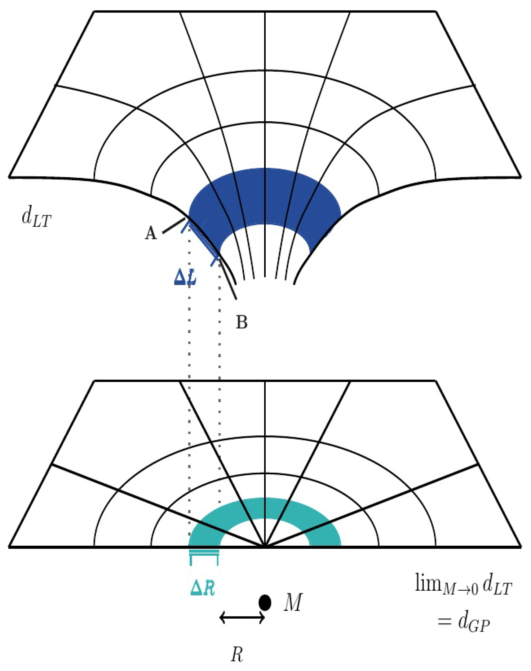
Figure 2.
Volume portions with speed (dotted) of homogeneous space with different normalized direction vectors of the velocity . The average of the velocities is zero. This causes global isotropy of space consisting of rapidly moving volume portions. As a consequence, this solves the space paradox.
Figure 2.
Volume portions with speed (dotted) of homogeneous space with different normalized direction vectors of the velocity . The average of the velocities is zero. This causes global isotropy of space consisting of rapidly moving volume portions. As a consequence, this solves the space paradox.
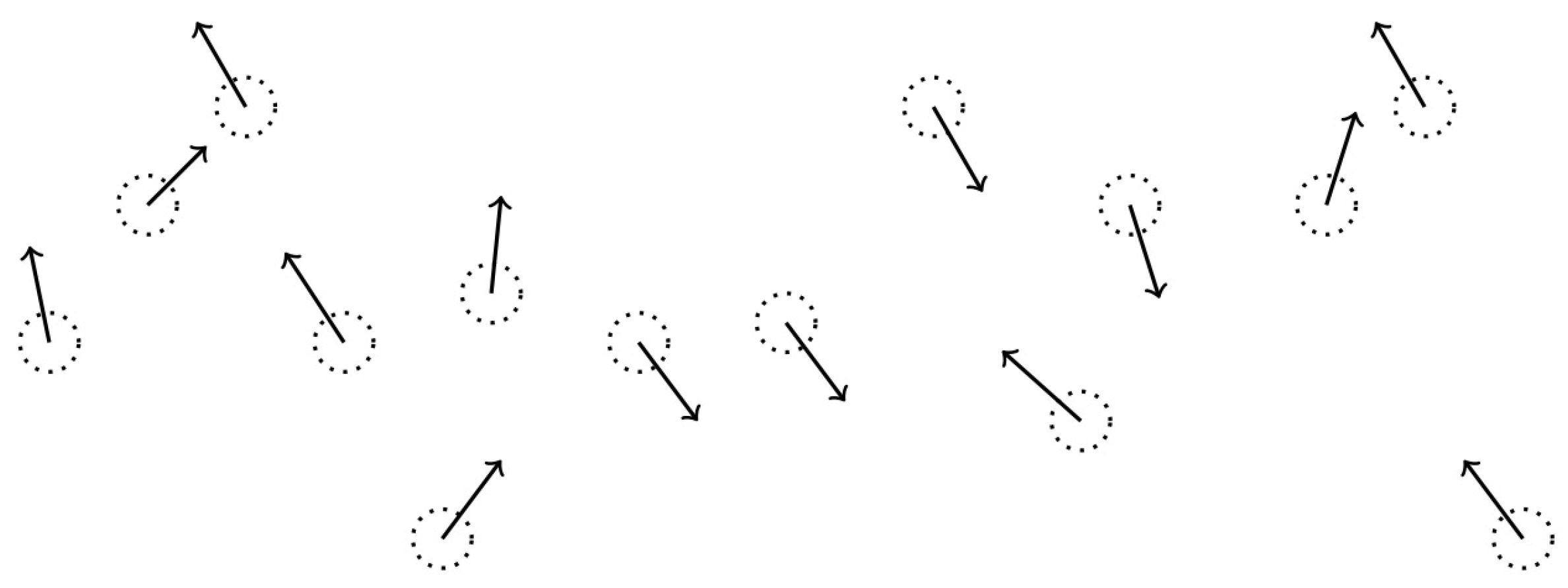
Figure 3.
Volume portions (VPs) with speed with different velocities : In general, each VP can include a change as marked at the left. In principle, each VP can be characterized very precisely by that change. For instance, the change of a VP moves with its velocity , and typically, it has a quadrupolar structure. A dipolar structure is excluded, as volume cannot be negative. At the right, these changes are indicated by wiggly lines, for simplicity. The average of the velocities is zero. This causes global isotropy of space consisting of volume portions with speeds . Therefore, this solves the space paradox.
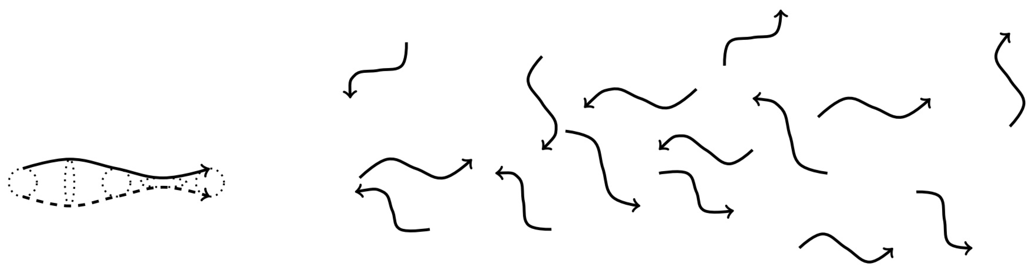
Figure 4.
A VP with a relative additional volume with a local maximum is shown as a function of location L and time . Thereby, the location L summarizes the three-dimensional vector in such a manner, that the length of the path of the VP is described by L.
Figure 4.
A VP with a relative additional volume with a local maximum is shown as a function of location L and time . Thereby, the location L summarizes the three-dimensional vector in such a manner, that the length of the path of the VP is described by L.

Figure 5.
In the vicinity of a field generating mass M, the space is curved (upper map), and in the limit , the space is flat (lower map), see Fig (Figure 1). The physical situation is expressed with help of a field in the right part.
Figure 5.
In the vicinity of a field generating mass M, the space is curved (upper map), and in the limit , the space is flat (lower map), see Fig (Figure 1). The physical situation is expressed with help of a field in the right part.
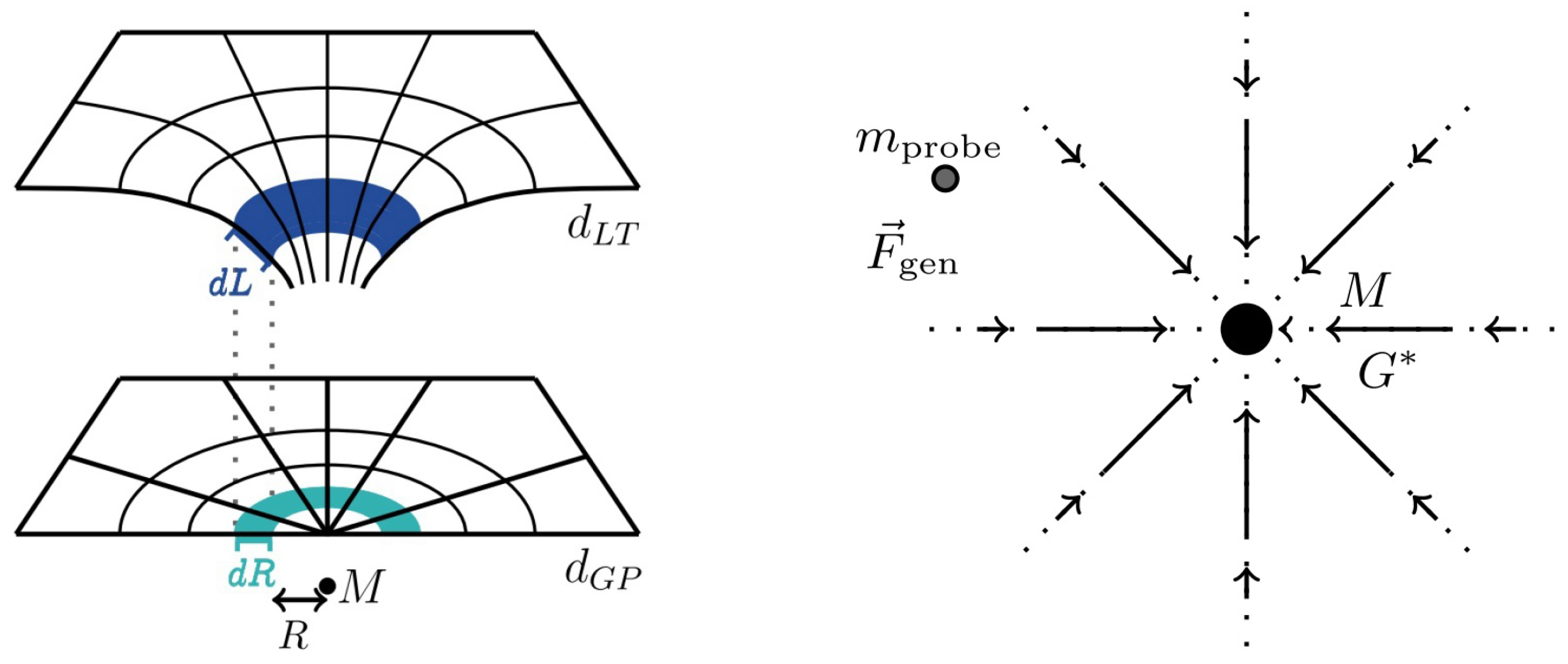
Figure 6.
A mass M (dark gray) in a shell at a radius R is lifted to a radius as follows: Differential parts are lifted, while the rest is still at R. Thereby the field (medium gray) in the shell with radius R and thickness becomes zero, when the whole mass is at .
Figure 6.
A mass M (dark gray) in a shell at a radius R is lifted to a radius as follows: Differential parts are lifted, while the rest is still at R. Thereby the field (medium gray) in the shell with radius R and thickness becomes zero, when the whole mass is at .
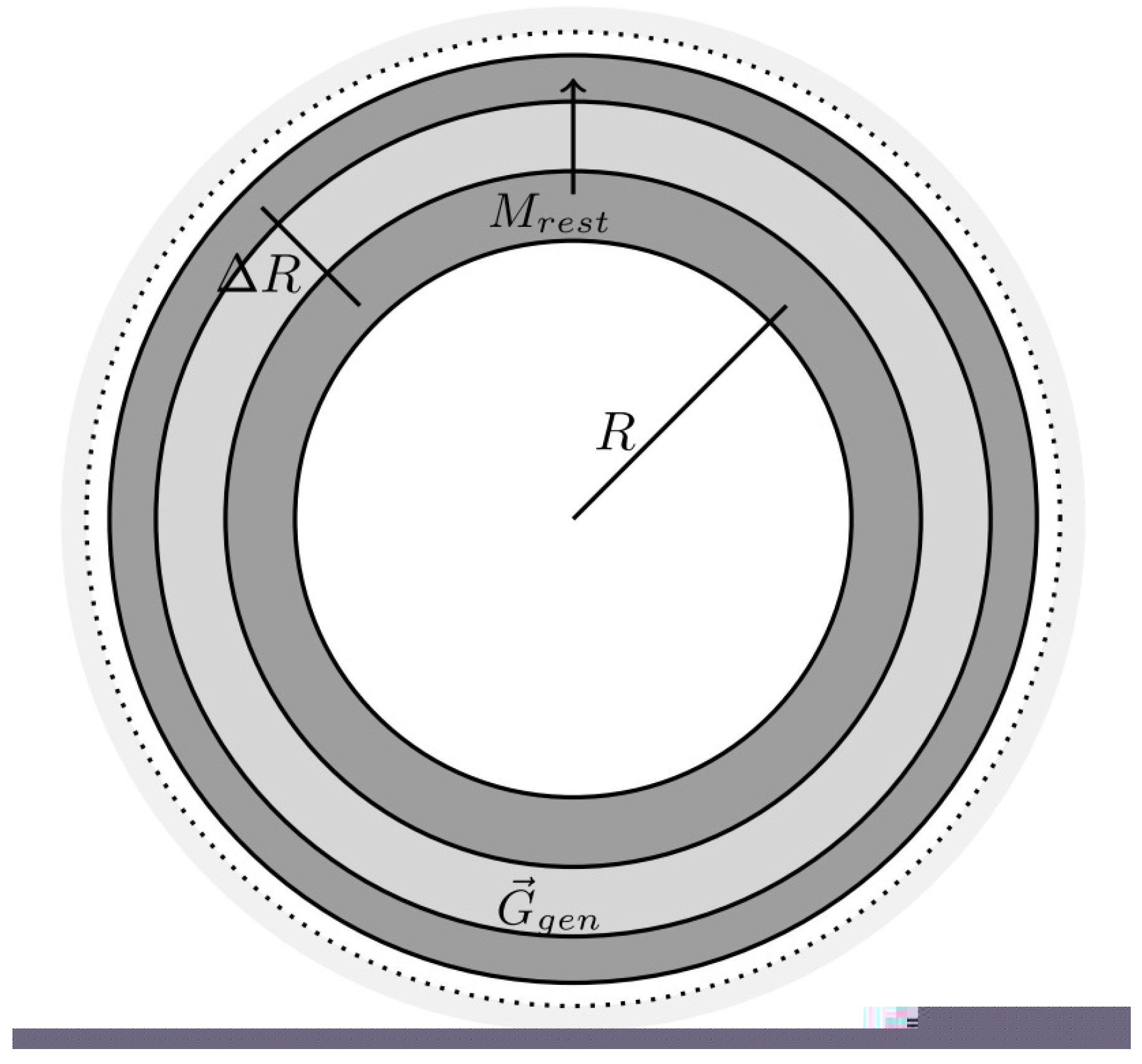
Figure 7.
The energy density in a shell at a distance R from has a dynamic mass . It generates rates , that propagate in the form of VPs or RGWs in all directions in the same manner.
Figure 7.
The energy density in a shell at a distance R from has a dynamic mass . It generates rates , that propagate in the form of VPs or RGWs in all directions in the same manner.
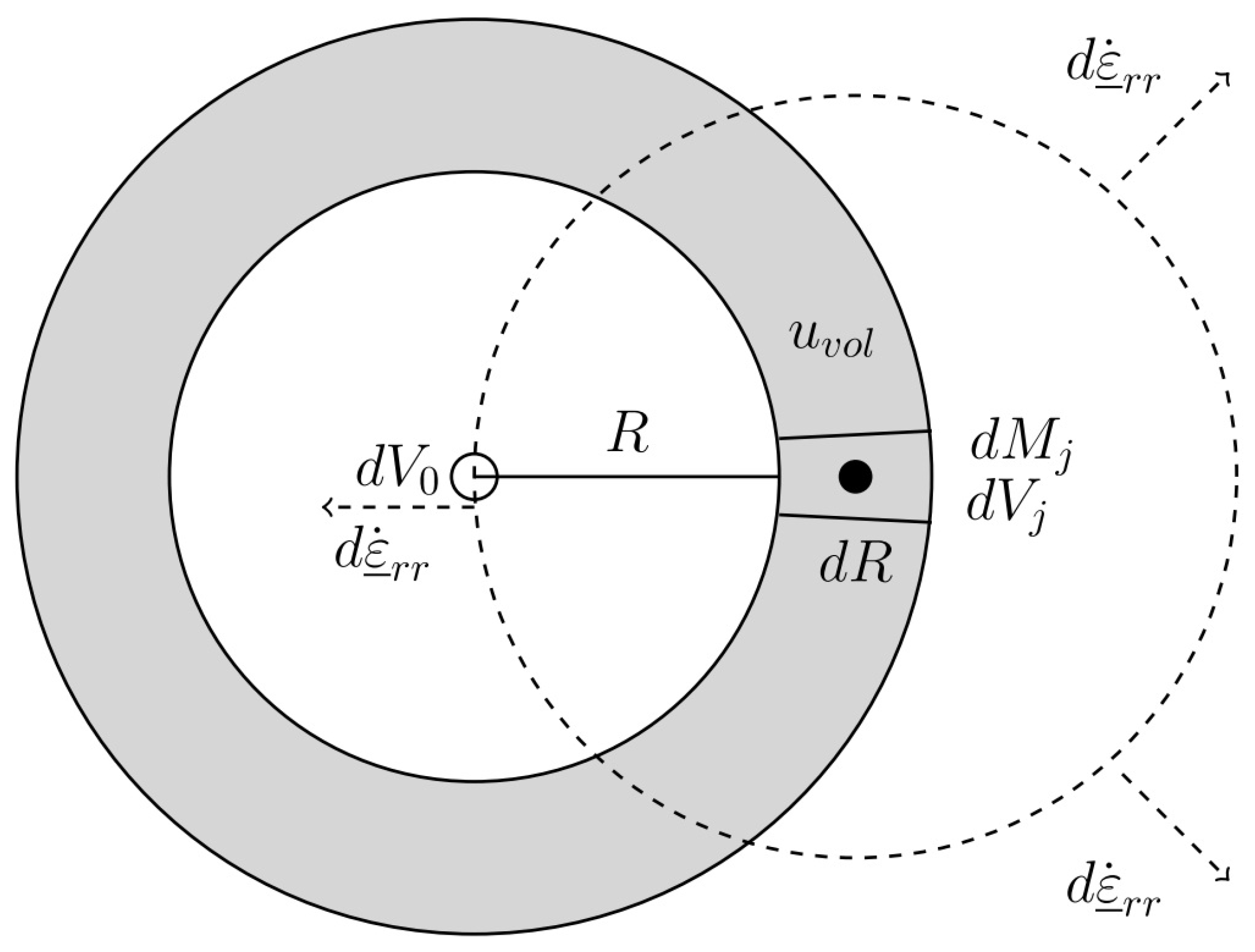
Figure 8.
Local densities are observed in boxes. The evaluation provides the following quantities: the averaged or homogeneous density , the local difference = , and the relative difference, the overdensity .
Figure 8.
Local densities are observed in boxes. The evaluation provides the following quantities: the averaged or homogeneous density , the local difference = , and the relative difference, the overdensity .
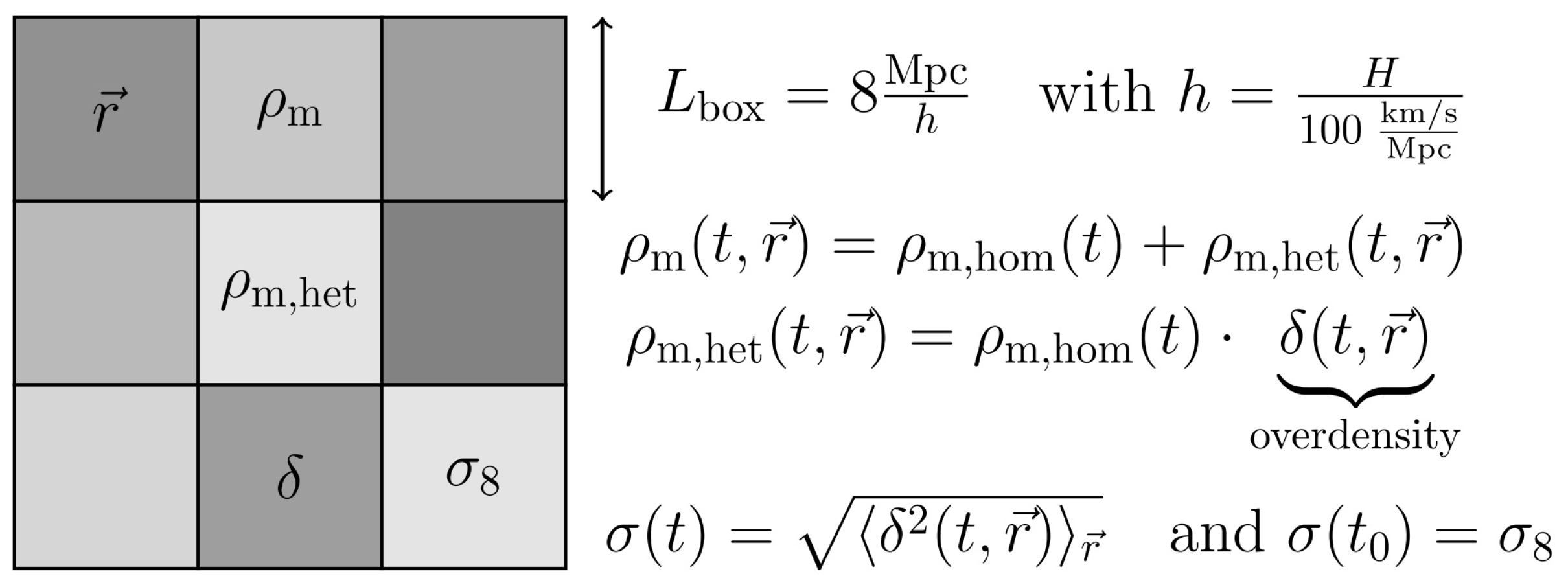
Figure 9.
Observed values and derived values of as a function of . Probes:×, megamaser [122]. ★, distance ladder with supernovae of type Ia [13,123], [124] most precise evaluation. ⧫, starburst galaxies [126]. o, baryonic acoustic oscillations, BAO [127,128]. •, weak gravitational lensing and galaxy clustering [129]. , strong gravitational lensing [130]. ⋄, gravitational wave [131]. ⊗, old galaxies or stars [132], (Tab. 1). □, surface brightness [133]. filled pentagon, CMB [22]. Derived from the VD: This theoretical curve (densely dotted) uses the calendar date , as this cannot be derived from fundamental physics. Thereby, theoretical values inherit the corresponding error of measurement of the used CMB value (loosely dotted). Measured and derived values are in precise accordance within the error of measurement.
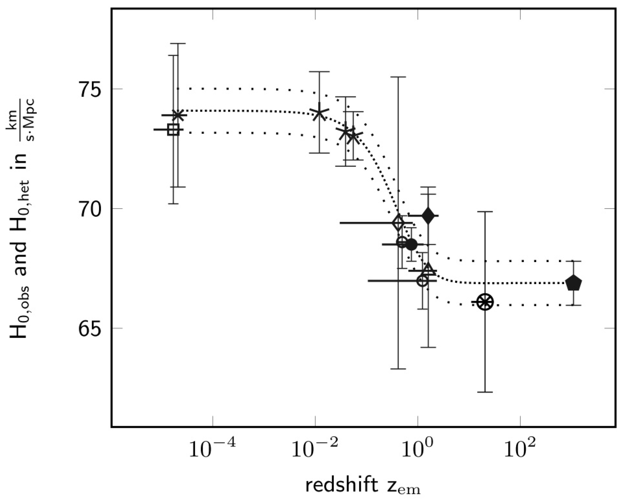

Table 1.
Expectation values of fields and the standard deviation or uncertainty of the field of the field. Hereby, the expectation value is abbreviated by .
Table 1.
Expectation values of fields and the standard deviation or uncertainty of the field of the field. Hereby, the expectation value is abbreviated by .
| object | state | |||||
| coherent | - | - | ||||
| number | 0 | 0 | 0 | |||
| coherent | 0 | |||||
| coherent | 0 | 0 | 0 |
Disclaimer/Publisher’s Note: The statements, opinions and data contained in all publications are solely those of the individual author(s) and contributor(s) and not of MDPI and/or the editor(s). MDPI and/or the editor(s) disclaim responsibility for any injury to people or property resulting from any ideas, methods, instructions or products referred to in the content. |
© 2025 by the authors. Licensee MDPI, Basel, Switzerland. This article is an open access article distributed under the terms and conditions of the Creative Commons Attribution (CC BY) license (http://creativecommons.org/licenses/by/4.0/).
Copyright: This open access article is published under a Creative Commons CC BY 4.0 license, which permit the free download, distribution, and reuse, provided that the author and preprint are cited in any reuse.


