1. Introduction
Coastal wetlands are more than just where land meets the sea; they are fundamental to the planet's ecological health [
1,
2]. The wetlands of Hangzhou Bay, for example, sit right in the middle of the East Asian–Australasian Flyway, a critical rest stop and feeding ground for over a million migratory waterbirds each year. The health of these wetlands directly impacts the survival of countless shorebirds like plovers and sandpipers, along with various geese and ducks [
3,
4].At the heart of this ecosystem are the macrobenthos—the small creatures living in the sediment. These organisms are not just a key part of the food web, cycling materials and energy, but they're also the primary food source that sustains the rich diversity of waterbirds [
5,
6]. But in recent years, this delicate balance has been thrown off by intense human activity and invasive species [
7].
One of the most aggressive invaders in China's coastal mudflats is
Spartina alterniflora, or smooth cordgrass. Since it was first introduced, it has spread like wildfire. In the Hangzhou Bay area, its incredible adaptability and rapid reproduction have allowed it to form dense, uniform fields, fundamentally changing the native ecosystem in several ways [
8,
9]. The plant's thick canopy and sprawling root systems alter water flow and sediment patterns, causing the mudflats to rise and changing the soil composition [
10]. Even more concerning, the invasion leads to habitat homogenization. By changing the sediment's physical and chemical properties and outcompeting native plants, S. alterniflora triggers major shifts in the macrobenthic communities. Most research shows that biodiversity drops sharply in invaded areas. This ecological decline directly cuts into the food supply for migratory birds, jeopardizing the entire flyway. That said, some studies do point out that these effects can vary depending on the context and across larger areas [
11].To fight this ecological crisis, large-scale S. alterniflora removal projects have been rolled out along China's coasts. Of all the techniques, physical tilling is one of the most common because it’s straightforward and gets fast results [
12]. This method tears out the invasive plants and mixes the leftover debris back into the sediment, which changes the area's nutrient levels as it decomposes. Yet, while the native plants might bounce back quickly, the response from the macrobenthic communities is often unpredictable and all over the map [
11,
13].
Research on how managing
Spartina alterniflora affects coastal ecosystems seems a bit lopsided. While plenty of studies have looked at plant succession and changes in the landscape, we still don't have a solid grasp of how bottom-dwelling marine animals (macrobenthos) bounce back after
Spartina is removed (Liu et al., 2023).Some reports suggest these animal communities do recover, but what’s actually driving that recovery is still murky. We aren't sure which environmental factors are most important or how the process works, and results often vary from place to place or depend on the methods used [
14]. This is especially true right after management, which is a key time for the ecosystem to heal. One of the biggest unanswered questions is whether the physical makeup of the sediment matters more than its nutritional content for these animals. Figuring this out is not just scientifically interesting; it could also help us fine-tune wetland restoration projects.
With that in mind, we chose the managed S. alterniflora zones on the southern coast of Hangzhou Bay for our study. We set up a comparison across three different habitats: patches of invasive S. alterniflora, restored areas now growing Scirpus mariqueter, and natural mudflats. By analyzing these sites, we examined the link between sediment properties and the animal communities living there.Our goal was to pinpoint which environmental factors—specifically the sediment's structure versus its food content—most influence the return of macrobenthic species and their overall biomass. The findings should clarify how these ecosystems recover after intervention and provide a better scientific basis for managing coastal invasions and protecting bird habitats. At the end of the day, we hope this work offers a practical model for similar restoration efforts elsewhere in China.
2. Materials and Methods
2.1. Study Area and Experimental Design
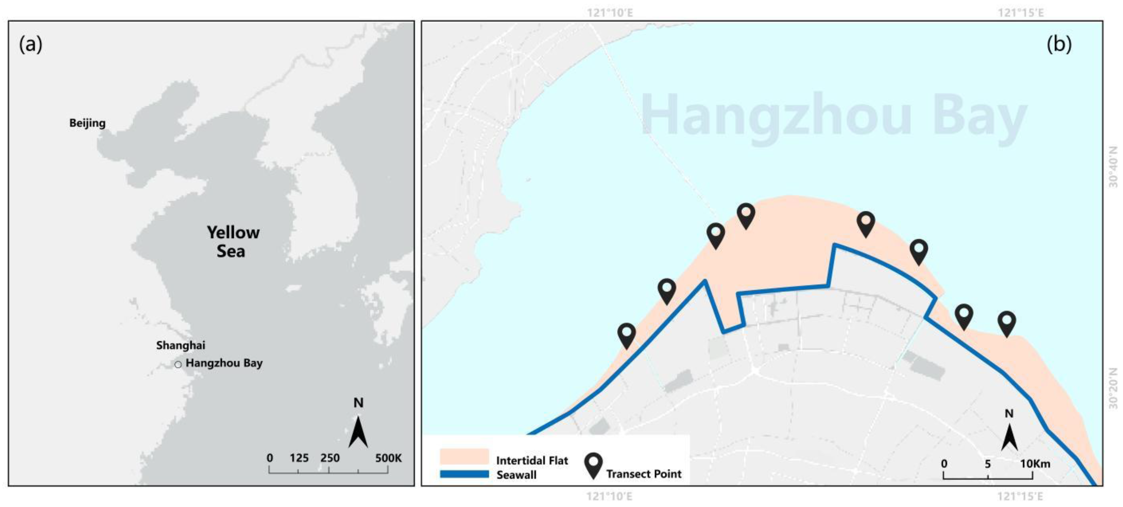
We conducted our study in the tidal flats of southern Hangzhou Bay (30°N, 121°E), a classic macrotidal estuary. This area is also a well-known stopover for migratory birds along the East Asian–Australasian Flyway [
3,
4].Our goal was to see how well the ecosystem was recovering after efforts to manage invasive
Spartina alterniflora. To do this, we used a space-for-time substitution method in April 2024. We focused on three habitat types: untouched stands of
S. alterniflora, areas where the native plant
Scirpus mariqueter had returned after tilling, and nearby native mudflats, which acted as our baseline for comparison. We set up 72 sampling units in total along the bay's southern coast—24 for each habitat type (Fig. 1).To make sure we were comparing apples to apples, we located the three habitat types next to each other along the same stretch of shoreline. This helped control for differences in tides and landscape. We also did all our sampling within the same season, waiting until the management project had settled and the weather was stable.
At each of the 72 units, we collected sediment and macrobenthos samples from a 10-meter radius. This ensured that our environmental and biological data came from the same spot. We were also careful to take replicate samples from areas that looked similar in terms of ground texture and small-scale bumps and dips, which helped reduce noise in the data. We sorted each sampling point into one of three categories based on what we saw:(1)S. alterniflora habitat: Areas with dense, continuous stands of the invasive grass, where you could see its rhizome root structures.(2)S. mariqueter habitat: Tidal flats covered by the native sedge S. mariqueter.(3)Mudflat: Bare, sandy-mud zones with almost no plants, typically crisscrossed by small tidal creeks.
Figure 1.
Overview of the study area:(a) Regional context along China’s east coast, indicating the position of Hangzhou Bay in the northern Yellow Sea–East China Sea sector. (b) Map of the southern shore of Hangzhou Bay: pink denotes the intertidal flat, blue traces the seawall, and black markers indicate fixed sampling sites. Each site comprised nine sampling units spanning one to three habitat types, with three replicate samples per unit.
2.2. Sediment Collection and Laboratory Analysis
We collected surface sediment from the center of each sampling unit with a 100 cm³ stainless steel corer. To get a representative sample and smooth out small-scale variations, we took three cores at each spot. We collected these along perpendicular lines, about 2–3 meters out from the central point, and mixed them together right away. We put the combined samples into pre-weighed, labeled plastic bags, kept them cool during transport, and started processing them within 24 hours of getting them back to the lab.In the lab, we first spread a small amount of each sample in an aluminum pan and pre-dried it at 55°C for 24 hours to stabilize its moisture content. We then fully dried it at 105°C until it reached a constant weight, which allowed us to calculate the water content (%) based on the Standard Methods 2540 protocol [
15]. To figure out the organic matter content, we burned another subsample in a muffle furnace at 550°C for at least six hours. The organic matter (g kg⁻¹) was simply the weight lost during burning, a method known as loss-on-ignition (LOI) that followed the quality control steps from Heiri et al.For particle size, we used laser diffraction [
16]. First, we broke up any clumps in the samples by sonicating them for two minutes with a dispersant. The instrument's volume-based results were converted to mass percentages, and we reported the data in three size groups: 0–2 μm, 2–20 μm, and 20–200 μm. Our whole process for calibration and reporting followed the ISO 13320:2020 standard [
17].
We used a water pycnometer to measure particle density (g cm⁻³), air-drying the samples at 60°C beforehand as recommended by ASTM D854[
18]. From there, we calculated total porosity (%) using the volumetric water content and the particle density. .Before running any analyses, we calibrated all our instruments for zero and drift according to the manufacturers' instructions. For quality control, we made sure the relative standard deviation for our replicate samples stayed below 5%. If any measurement fell outside that range, we repeated it.
2.3. Macrobenthic Fauna Sampling and Biomass Determination
To sample the small animals living in the sediment (the macrobenthos), we used a cylindrical corer with a 10 cm inner diameter, pushed 20 cm deep into the seafloor. At each location, we took three separate samples this way.we carefully mixed each sample with seawater and washed it through a 0.5-mm stainless steel sieve. Everything left on the screen—animals and bits of debris—was preserved in 75% ethanol and kept in a cool, dark place. For samples caked in a lot of clay, we gave them a quick, gentle rinse with fresh water before adding the ethanol. This simple step helped prevent tiny bits of animal tissue from flaking off with the clay during later lab work.
In the lab, we sorted the organisms under a stereomicroscope. We identified each one to the most specific taxonomic level possible but, at a minimum, placed them into one of four main groups:
Decapoda,
Gastropoda,
Bivalvia, and
Polychaeta. After counting every individual, we moved on to measuring their biomass.We determined the ash-free dry mass (AFDM)[
19], which is a standard way to measure the organic tissue of an organism. First, we dried the samples in an oven at 60°C until they reached a constant weight—this is the dry weight (DW). Then, we incinerated them in a furnace at 550°C for six hours. What’s left is just ash. The AFDM is simply the difference between the two (DW – Ash), weighing them one by one would have been prone to error. So, we grouped them by taxon, weighed them all together, and then divided by the number of individuals to get a reliable average. We also had to account for the ethanol preservative, which can affect mass. To do this, we briefly rinsed the specimens with distilled water and pre-dried them at 60°C for 12 hours just before the official weighing. As a quality check, every batch we processed included empty dishes and standard weights to make sure our measurements were consistent.Finally, we tallied the species richness (the number of different species) and total AFDM biomass for each of the four taxonomic groups. From there, we calculated the overall species richness and total biomass in grams per square meter (g m⁻²) for each sampling site.
2.4. Statistical Analysis
Our statistical analysis had four main parts. First, we tested for differences between the habitats. Next, we estimated the size of those differences. Then, we looked at the bigger picture of how the habitats were structured. And finally, we used machine learning to figure out what was driving the changes we saw. To make sure our results were repeatable, we used the same data version and random seed for all analyses.
For each sediment and macrobenthic measurement, we ran a one-way analysis of variance (ANOVA) with habitat type as the main factor. To see exactly which habitats differed, we followed up with Tukey's HSD test, which helps control for errors when you're doing a lot of comparisons.To get a real sense of how much things changed with management versus the invasion, we calculated the median differences between the
Scirpus and
Spartina habitats. We then built 95% confidence intervals for these differences and displayed them in forest plots [
20]. We used a bootstrap method to do this, resampling our data 3,000 times within each habitat to get a reliable estimate of the uncertainty (this approach follows the work of Efron & Tibshirani)[
20]. The mudflat habitat was kept as a reference point for general comparison but wasn't included in these specific calculations.We then used principal component analysis (PCA) to see if we could find underlying sediment patterns and how well the habitats separated from each other based on their overall characteristics [
21]. The analysis included grain-size data (after an isometric log-ratio transformation) and other physical and chemical variables. Before running the PCA [
22], we centered and scaled all variables. We created a biplot showing the first two principal components (PC1 and PC2), which included the individual samples and 95% confidence ellipses for each habitat. We then ran a PERMANOVA with 999 permutations to formally test if the habitat groups were truly different from one another [
23].
Finally, we wanted to pinpoint the key factors behind the recovery of the benthic community. To do this, we built two Gradient Boosting (XGBoost) models—one to predict total biomass and another for total species richness. After training the models, we used the SHAP framework to figure out which environmental features were most important and whether their effect was positive or negative [
24,
25,
26].
3. Results
3.1. Variation in Sediment Physicochemical Properties Among Habitats
As expected, the sediment properties differed noticeably across the three habitats (
Table 1).
The Scirpus mariqueter habitat was the most porous (62.21 ± 3.85%), followed by the mudflat (54.26 ± 2.16%), and finally the Spartina alterniflora habitat (42.53 ± 2.28%). A similar pattern appeared in water content, which was highest in the S. mariqueter habitat at 35.30 ± 2.63%. The mudflat and S. alterniflora habitat had nearly identical, lower water content (26.32 ± 4.92% and 25.67 ± 2.22%, respectively).
Interestingly, the trends for organic matter and particle density were reversed. The S. alterniflora habitat had the most organic matter (10.38 ± 1.83 g kg⁻¹), while the S. mariqueter habitat and mudflat were much lower and almost the same (7.27 ± 1.95 and 7.15 ± 1.05 g kg⁻¹). Particle density was also highest in the S. alterniflora habitat (2.76 ± 0.09 g cm⁻³) compared to the other two sites, which were again quite similar (2.66 ± 0.05 and 2.65 ± 0.05 g cm⁻³).
Looking at the grain-size structure, the S. alterniflora habitat and mudflat were dominated by fine particles. For instance, the 2–20 μm fraction made up over half the sediment in both areas (56.23 ± 11.14% and 55.08 ± 6.11%, respectively). In stark contrast, the S. mariqueter habitat was made up of much coarser material; its sediment was over two-thirds coarse particles (67.52 ± 6.79% in the 20–200 μm range), far more than either the mudflat (37.67 ± 6.44%) or the S. alterniflora habitat (31.39 ± 13.74%).
3.2. Variation in Benthic Community Richness and Biomass Across Habitats
As shown in
Table 2, we found clear patterns in community metrics across the three habitats. Total species richness was highest on the mudflat (12.58 ± 5.02), dropped in the
Scirpus mariqueter habitat (8.29 ± 2.46), and was lowest in the
Spartina alterniflora habitat (4.42 ± 2.10).
Looking at specific taxonomic groups, the differences were most obvious for Decapoda and Polychaeta . Decapod richness followed the same general pattern: highest on the mudflat (4.58 ± 2.21), lower in the S. mariqueter habitat (2.62 ± 1.71), and lowest in the S. alterniflora habitat (1.62 ± 1.21). Polychaete richness mirrored this trend, declining from the mudflat (3.54 ± 2.25) to the S. mariqueter habitat (1.71 ± 1.30) and finally to the S. alterniflora habitat (0.83 ± 0.92). For Gastropoda and Bivalvia, richness was generally higher in both the mudflat and S. mariqueter zones compared to the S. alterniflora habitat.
total biomass showed the opposite trend. It peaked in the S. mariqueter habitat (21.97 ± 7.99 g m⁻²), followed by the mudflat (12.89 ± 5.35 g m⁻²), and was far lower in the S. alterniflora habitat (1.49 ± 1.21 g m⁻²). This pattern held for most individual taxonomic groups, including decapods, gastropods, and bivalves. The only exception was polychaete biomass, which was fairly similar between the S. mariqueter habitat and the mudflat (6.96 ± 5.58 and 4.95 ± 4.14 g m⁻², respectively), though both were still much higher than in the S. alterniflora habitat (0.15 ± 0.18 g m⁻²).
3.3. Key Sediment Properties
Sediment metrics differed clearly between the
Scirpus mariqueter and
Spartina alterniflora habitats (
Table 3). The
S. mariqueter habitat had much higher total porosity and water content (61.56% vs. 42.48% and 35.62% vs. 24.80%, respectively). In contrast, the
S. alterniflora habitat contained more organic matter (10.70 vs. 7.73 g kg⁻¹).
Looking at grain size, the S. mariqueter habitat contained fewer fine particles (0–2 μm and 2–20 μm) but a much larger share of coarser particles (20–200 μm) than the S. alterniflora zone. Particle density was also slightly lower in the S. mariqueter habitat (2.67 vs. 2.75 g cm⁻³).
The mudflat’s characteristics generally fell between the two vegetated habitats. Its share of fine particles (2–20 μm) resembled that of the S. alterniflora habitat, while its coarse particle fraction was closer to the S. mariqueter habitat. In short, the S. mariqueter habitat was more porous, held more water, and was composed of coarser sediment, whereas the S. alterniflora habitat was finer-grained with higher organic content.
3.4. Comparison of Sediment Properties and Principal Component Structure
- 1)
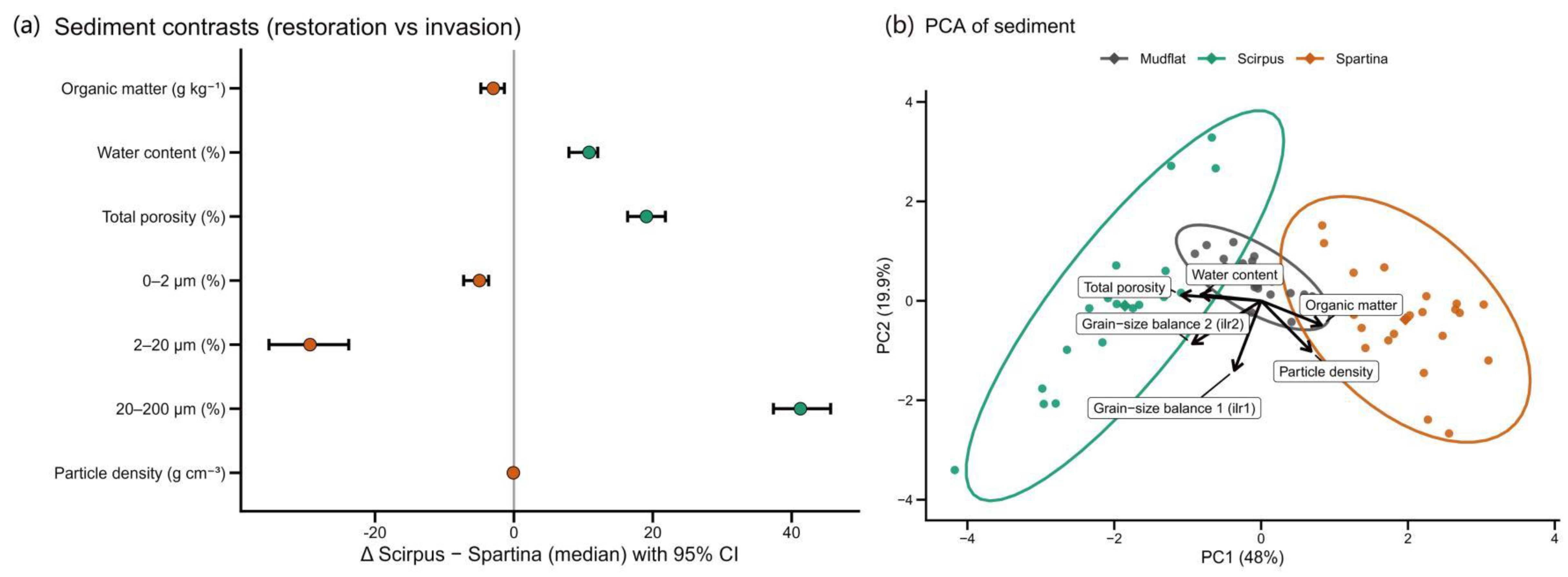
Contrasting Scirpus and Spartina Habitats
The forest plot (Fig. 1a) gives us a direct comparison of the soil properties in the Scirpus and Spartina habitats. The most striking difference was in the sediment grain size. The Scirpus habitat had a much higher proportion of coarse grains (20–200 μm), about 41.26 percentage points more than the Spartina habitat (95% CI: 37.37–45.61). Conversely, it had significantly fewer fine grains (2–20 μm), with a deficit of around 29.36 percentage points (95% CI: -35.27 to -23.78).Physical properties also differed. Scirpus soils were more porous and held more water, with total porosity and water content being higher by 19.08 and 10.83 percentage points, respectively. Looking at the chemistry, Spartina soils contained more organic matter (difference: -2.97 g kg⁻¹), while Scirpus soils had a slightly lower particle density (difference: -0.08 g cm⁻³).
Taken together, these results paint a clear picture. The
Scirpus habitat is defined by a coarser, more porous, and wetter substrate. In contrast, the
Spartina habitat has finer soil that is richer in organic matter. As one might expect, the bare mudflat sits somewhere in the middle (see
Table 3).
- 2)
Environmental Gradients Separating the Three Habitats
The PCA confirmed this separation, showing how the three habitats cluster based on their environmental profiles (Fig. 1b). The first principal component (PC1), which explains 48% of the total variance, effectively splits the habitats. Spartina samples group on the positive side of PC1, Scirpus samples on the negative side, and the mudflat samples hover near the center.
What drives this split? The loadings tell the story. The negative side of PC1, where Scirpus sits, is linked to higher porosity (-0.54), water content (-0.41), and a grain-size balance favoring coarse particles (ilr2, -0.47). The positive side, home to Spartina, is associated with higher organic matter (+0.41) and particle density (+0.34). This lines up perfectly with what we saw in the forest plot: Scirpus is coarse and porous, while Spartina is fine-grained and organic-rich. The second axis, PC2, was mostly driven by another grain-size balance (ilr1, -0.70). Once again, the mudflat occupies an intermediate position along these environmental gradients.
3.5. Benthic Community: Median Distribution by Habitat and Management-Induced Gains (Δ Scirpus − Spartina)
Looking at the median values from
Table 4, a clear pattern in species richness emerges across the habitats. The mudflat was the most diverse with 14 species, followed by the native
Scirpus mariqueter habitat (9 species), and finally the invasive
Spartina alterniflora habitat, which hosted only 5 species. This means the restored S. mariqueter areas supported four more species than the
S. alterniflora patches—a welcome sign of recovery.
Then we dig into specific animal groups,
Decapoda and
Polychaeta showed the biggest jumps. For instance,
Decapoda richness climbed from just one species in
S. alterniflora beds to three in
S. mariqueter and five in the mudflats. We saw a similar trend for
Polychaeta, going from zero to two, and then to four species across the same habitats. Gastropods and Bivalves also increased, just not as dramatically. As
Figure 2a illustrates, the story here is one of low species counts in the invasive grass, a partial recovery in the restored native grass, and a high baseline in the untouched mudflat.
Biomass tells a similar story. The mudflat again came out on top with a median biomass of 16.43 g m⁻², while the S. mariqueter and S. alterniflora habitats had 11.75 g m⁻² and a meager 1.36 g m⁻², respectively. The recovery in the S. mariqueter habitat was substantial, adding over 10 g m⁻² in biomass compared to the invasive grass beds. Bivalves were the star performers here, their biomass jumping from 0.26 g m⁻² in the S. alterniflora habitat to 3.90 g m⁻² in the restored S. mariqueter habitat. Decapods and Gastropods also saw large gains, though Polychaete biomass remained low overall (Fig. 2b).
Putting it all together, the restored S. mariqueter habitat clearly represents a gain for the ecosystem. Compared to the invasive S. alterniflora, it supports both more species (+4) and significantly more biomass (+10.38 g m⁻²). Most of this improvement comes from the return of Bivalves, Decapods, and Gastropods, while Polychaetes contributed more to the species count than to the overall weight.
Figure 3.
a. Boxplots with overlaid points of benthic species richness across three habitats, showing sample distribution and dispersion for Decapoda, Gastropoda, Bivalvia, Polychaeta, and total richness.b. Boxplots with overlaid points of benthic biomass across three habitats, using a logarithmic scale to display cross-order differences for Decapoda, Gastropoda, Bivalvia, Polychaeta, and total biomass.
3.6. Key Drivers of Benthic Recovery (XGBoost–SHAP)
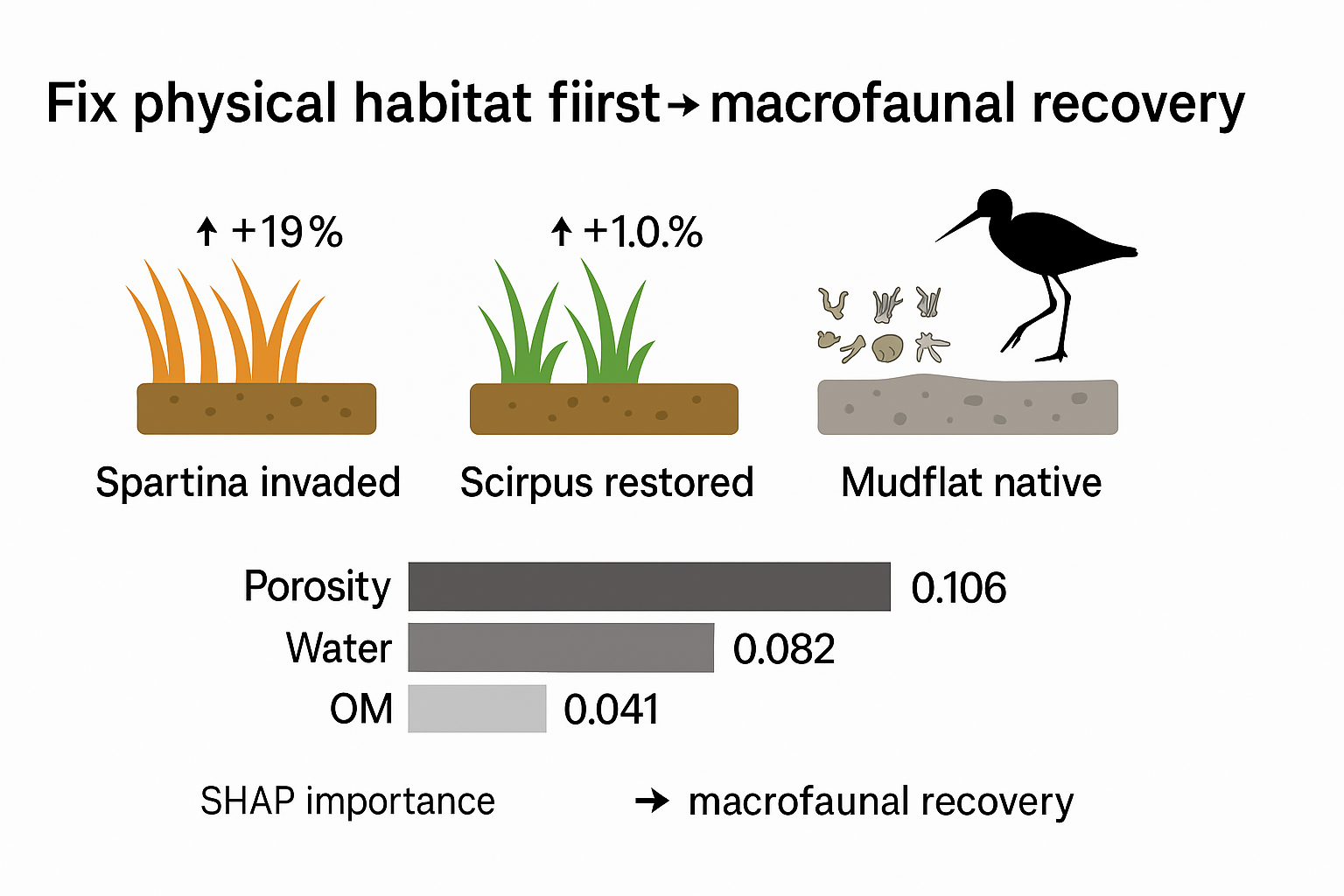
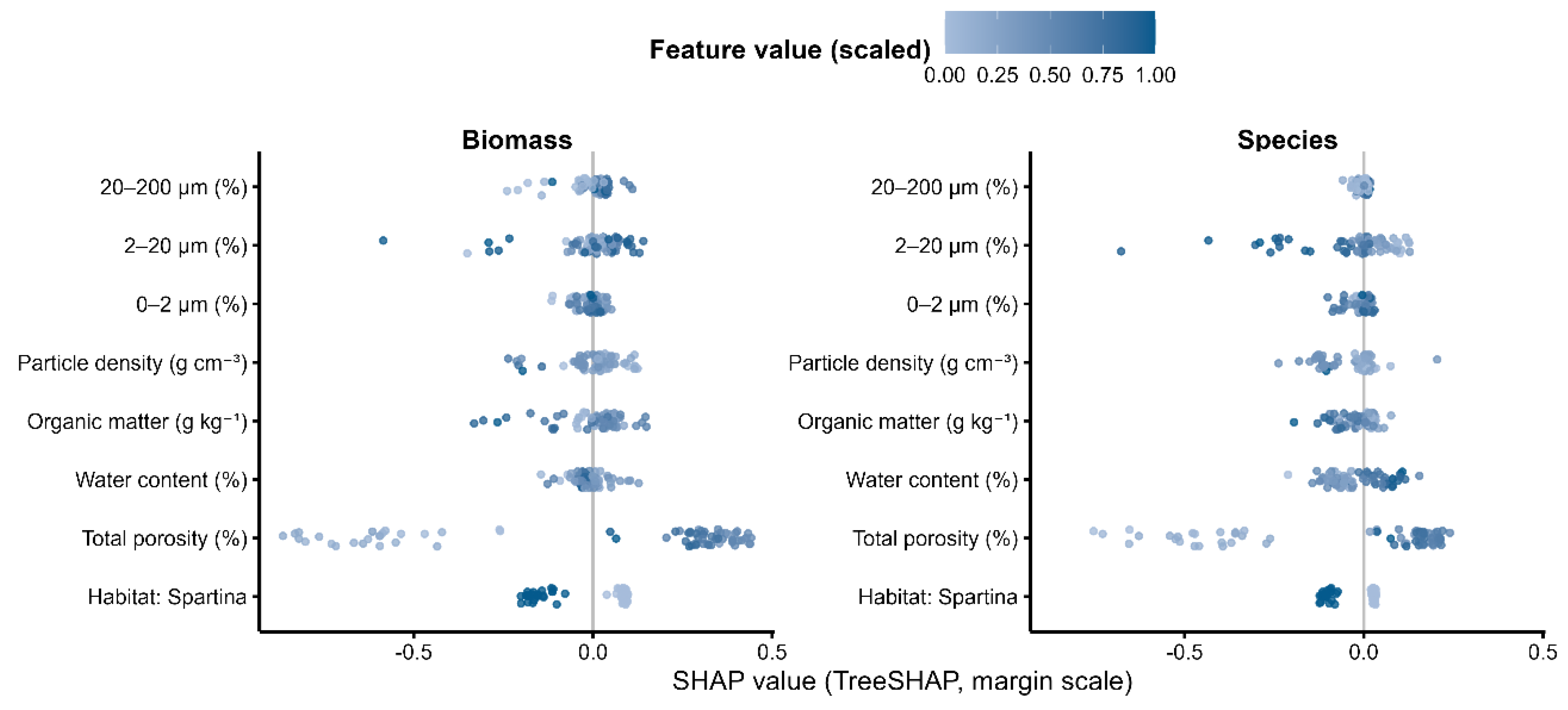
Our analysis of the gradient boosting models shows that sedimentary environmental factors were the main drivers of benthic recovery, measured by both total biomass and species richness (
Table 5, Fig. 3). For both metrics, total porosity and water content clearly stood out. According to the SHAP importance scores, total porosity ranked first, with a score of 0.106 for biomass and 0.092 for species richness. Water content was a close second, scoring 0.082 for biomass and 0.084 for species richness.
Figure 4.
SHAP beeswarm plots from XGBoost models, with Biomass and Species panels. The x-axis shows SHAP values (margin scale), indicating the change in model output associated with a variable at a given observation: values to the right indicate positive contributions and to the left indicate negative contributions; the vertical gray line denotes zero. Each point is an observation, colored by the standardized value (0–1) of that variable to illustrate how effect direction varies with the feature value; the cloud of points for a variable depicts its effect distribution. Variables are ordered from top to bottom by global importance (mean SHAP), grouped as Habitat → Sediment properties → Grain size. “Habitat: Spartina” is a dummy variable (1 = Spartina habitat, 0 = other habitats).
Other factors, like grain size and physicochemical indicators, also played a part, just not as significant. The finest particle sizes (0–2 μm and 2–20 μm) had a moderate impact on both biomass and species richness. Organic matter and particle density were even less influential.Looking at the direction of these effects, we found some consistent patterns. Higher total porosity and water content were almost always linked to better community recovery—that is, more biomass and more species. This makes intuitive sense, as looser, wetter sediment often supports more life. On the other hand, higher particle density had a negative effect on both biomass (−0.028) and species richness (−0.031). This fits with what we've seen in S. alterniflora habitats, where denser sediment typically has lower porosity. Organic matter had a small, positive influence, but its role was clearly secondary to that of porosity and water content.
The effects of grain size were a bit more complex. The finest particle fractions (0–2 μm and 2–20 μm) generally had a weak negative impact on both biomass and species richness. Interestingly, some variables showed high importance but had an average effect close to zero. The 2–20 μm fraction for species richness is a good example. This suggests that the effect might not be straightforward—it could be positive in some ranges and negative in others, a pattern also hinted at in the SHAP beeswarm plots.
So, to put it all together: at our study sites, sediments with higher porosity and water content supported richer and more abundant macrobenthic communities. In contrast, denser sediments with a higher proportion of fine particles were generally linked to poorer recovery. These findings were remarkably consistent across both models, solidifying the primary role of porosity and water content. The other variables—organic matter, grain size, and particle density—formed a secondary tier of influence. We also cross-checked these findings using permutation importance, which confirmed that total porosity and water content were indeed the most important factors.
4. Discussion
4.1. Fundamental Shifts in Habitat Physical Structure
When
Spartina alterniflora invades a tidal flat, it doesn't just add a new plant—it fundamentally re-engineers the ecosystem. Our experiments showed a clear split in habitat types. The areas taken over by
S. alterniflora became noticeably more compact. They had lower porosity, held less water, and were dominated by fine-grained particles. This isn't a local quirk; other recent studies have consistently found the same pattern where
Spartina invasion leads to denser sediment and alters everything from organic carbon and nitrogen cycles to the way water moves through the mud [
26,
28,
32,
34].
So, what's causing this? It comes down to the plant's dense network of roots and rhizomes [
28,
32]. This root system acts like a net, trapping fine particles from the water and stabilizing the sediment [
28,
29,
33]. Over time, this raises the elevation of the mudflat, reduces water flow and aeration, and creates a compacted, fine-grained substrate. Interestingly enough, the restored
Scirpus mariqueter habitat showed a completely different set of physical traits. It had higher porosity and water content, with a greater share of coarse sand. This combination of improved physical, hydrodynamic, and oxygenated conditions is a good sign. Recent assessments suggest this kind of environment is much better at supporting the return of benthic communities and restoring the flat's ecological functions [
29,
31,
33] . From a restoration standpoint, this also tells us that ecosystems don't always bounce back to their original state. Instead, they might follow new paths and develop unique characteristics.
Our results suggest that for macrobenthos to recover, the physical structure of the sediment is more important than the amount of organic matter available. It seems that in the Hangzhou Bay tidal flats, having the right kind of physical space to live in is a more immediate need for these communities than the food supply. This idea is backed by other studies showing that benthic communities tend to thrive where there's more sand, less fine silt and clay, and better oxygen and water flow near the sediment surface [
30,
35]. They struggle in compacted, low-oxygen substrates .Think of it as environmental filtering: the dense, suffocating sediment created by
Spartina simply weeds out many bottom-dwelling organisms. In contrast, the improved physical conditions in the restored
Scirpus mariqueter habitat offer a much more welcoming foundation for these creatures to recolonize and rebuild their community [
35].
At the end of the day, a rule of thumb for restoring dynamic coastal systems is emerging: first, fix the physical problems. Things like porosity, water content, grain size, and water flow are often the primary bottlenecks. Only after these physical foundations are in place can efforts to improve nutrient levels and resources truly succeed. Our findings from this region fit squarely within this growing international consensus: the recovery of the sediment's physical properties goes hand-in-hand with the recovery of the benthic community [
33] .
4.2. Differential Response Mechanisms of Macrobenthic Communities
The way macrobenthos bounced back in this study gives us a new look into the feedback loops that kick in after we try to manage invasive species. A key takeaway is that tilling
Spartina alterniflora left behind a huge amount of litter, which then decomposed and pumped a lot of organic matter into the tidal flat system. As
Table 1 shows, the organic matter in the old
S. alterniflora habitat was much higher than elsewhere—a direct result of all that biomass breaking down right after the tilling [
36,
37].You might think all this extra food would have sparked a widespread recovery of macrobenthos, but that’s not what happened. Our analysis pointed to a different culprit: the physical structure of the sediment, not the amount of organic matter, was the real driver behind the recovery patterns [
38,
39]. This seems like a paradox, but it likely comes down to an ecosystem trade-off. While the decaying litter provided a short-term food surplus, its benefits were cancelled out by the dense, low-oxygen soil left behind by
S. alterniflora [
40]. For most bottom-dwelling creatures, having enough space and oxygen to live is a more immediate problem than finding food .
This finding adds an interesting layer to the classic competition exclusion theory, which usually just focuses on the fight for food. It suggests that when an ecosystem is recovering from an invasive plant, the first hurdle is fixing the physical stress, which paves the way for the community to reassemble. We saw this in the
Scirpus mariqueter habitat. There, the sediment structure had improved, and the macrobenthic community developed unique transitional features, making it different from both the physically stressed invaded areas and the open mudflats. This pattern seems to support the Intermediate Disturbance Hypothesis, where our management actions created a unique niche where physical filtering was the main game in town.When we compare our work to previous studies, the importance of context really stands out. Many studies point to how invasive plants change sediment chemistry, but our work in the highly dynamic Hangzhou Bay highlights that physical changes can be the deciding factor. We also noticed that polychaetes and bivalves responded differentl [
41,
42,
43]y. Polychaete species returned quickly, but it was the bivalves that contributed most to the overall biomass. This goes against the common assumption that these two groups react similarly to environmental shifts and probably reflects different life strategies and tolerances .
At the end of the day, ecosystem recovery is a process with multiple stages. In the Hangzhou Bay tidal flats, the organic matter from dead
S. alterniflora laid the resource groundwork for recovery. But for that to matter, a key condition had to be met first: the physical structure of the sediment needed to improve. Only after the physical stress was relieved could the benefits of the extra resources start to show up in later successional stages. This assembly process, driven by physical filtering, gives us a solid theoretical basis for predicting long-term ecosystem changes and for planning restoration strategies that work in phases [
44].
4.3. Understanding the Ecological Process of Invasion and Recovery from a Physical Structure Perspective
Our findings suggest that the biggest ecological impact of a
Spartina alterniflora invasion—and its later removal—might be how it tears up and rebuilds the physical structure of sediment [
45,
46]. We've known for a while that
S. alterniflora has geomorphological effects, like trapping sediment and stabilizing tidal flats. But this new insight goes deeper, showing how the plant fundamentally alters the physical livability of benthic habitats. The invasion isn't just about resource competition; it's about the physical loss of living space. Consequently, successful management isn't just about removing the plant. Critically, it depends on reopening that compressed physical space for life to return [
47].
Looking at the problem from this physical perspective adds an important layer to classical invasion ecology theory. It tells us that in high-energy tidal flats like Hangzhou Bay, where physical disturbance is the norm, an invader's ability to change the substrate itself can outweigh its short-term effects on resource availability [
48,
49]. Our study points to a likely sequence for ecosystem recovery: rebuilding the physical habitat is a necessary first step, though it's not the only thing needed for biological communities to bounce back. This explains why, even with plenty of organic matter available after the invasive plants are removed, the recovery of macrobenthic communities still hinges on improvements in physical factors like sediment porosity and water content [
50,
51].What’s more, the fact that different macrobenthic groups respond differently to these physical improvements shows that ecological restoration isn't a simple, balanced process. This uneven recovery suggests the post-management ecosystem is charting a new, nonlinear path forward rather than just returning to a pristine, historical state. This transition is shaped by a mix of drivers, including physical filtering, limitations in the local species pool, and niche dynamics [
52].
Ultimately, this study reframes the
S. alterniflora invasion and its management in Hangzhou Bay. Instead of seeing it as a simple species-for-species swap, we should see it as a process that re-engineers the ecosystem's physical foundation, which in turn drives community succession [
53,
54]. This framework connects the dots from habitat modification to community response. It also gives us a new conceptual tool for predicting the long-term outcomes of management projects and for comparing the impacts of different invasive plants in coastal zones worldwide.
5. Management Implications and Research Limitations
Based on our findings, managing coastal wetlands needs to be about more than just replanting vegetation; we also have to consider how the sediment's physical structure is changing over time. The data shows a clear link between the recovery of bottom-dwelling creatures (macrobenthos) and physical factors like sediment porosity and water content. This suggests that we should start tracking these physical properties to get a real sense of whether our management efforts are actually working.
For restoration projects on the ground, it makes sense to use native plants that are good at improving the sediment structure right from the start. Think of them as the pioneers of the rehabilitation effort. We also noticed that different ecological groups bounce back at different speeds. So, instead of a one-size-fits-all assessment, we should probably set up phased evaluation protocols that account for these different recovery timelines.It's important to remember, though, that these conclusions come from a single study in one specific place and time. We need to see if they hold true across different regions and over longer periods. Tidal flat recovery is a complex puzzle, influenced by everything from water flow to sediment types, and our work has only uncovered a few pieces of that puzzle.
Future research should look at a wider range of environmental factors and track these sites long-term. Only then can we get a complete picture of how these coastal wetlands truly heal. Ultimately, these insights offer a better foundation for wetland restoration ecology and give managers scientifically-backed ideas for improving how they work.
Author Contributions
Dingda Chen: conceptualization, data curation, formal analysis, methodology, software, validation, visualization, writing – original draft.Chuanliang Li:formal analysis,methodology,supervision,writing – review & editing.Xinli Zhang: funding acquisition, Investigation,.Xuexin Shao: supervision, writing – review & editing.Ming Wu: funding acquisition.Shengwu Jiao: conceptualization, methodology, investigation, supervision, validation, funding acquisition, writing – review & editing.
Funding
This work was supported by the Fundamental Research Funds for the Central Nonprofit Research Institution (CAFYBB2025ZC009) and the Pioneer and Leading Goose R&D Program of Zhejiang Province (Grant No. 2024C02002)..
Data Availability Statement
Data will be made available upon request.
Acknowledgments
Xiaohong Zhu and Xijuan Xu helped on the field work.
Conflicts of Interest
The authors declare no conflicts of interest.
References
- Murray, N. J.; Worthington, T. A.; Bunting, P.; Duce, S.; Hagger, V.; Lovelock, C. E.; Lyons, M. B. The global distribution and trajectory of tidal flats. Nature 2019, 565, 222–225. [Google Scholar] [CrossRef] [PubMed]
- Murray, N. J.; Worthington, T. A.; Bunting, P.; Duce, S.; Hagger, V.; Lovelock, C. E.; Lyons, M. B. High-resolution mapping of losses and gains of Earth’s tidal wetlands. Science 2022, 376, 744–749. [Google Scholar] [CrossRef] [PubMed]
- Studds, C. E.; Kendall, B. E.; Murray, N. J.; Wilson, H. B.; Rogers, D. I.; Clemens, R. S.; Fuller, R. A. Rapid population decline in migratory shorebirds relying on Yellow Sea tidal mudflats as stopover sites. Nat. Commun. 2017, 8, 14895. [Google Scholar] [CrossRef]
- Cai, S.; Mu, T.; Peng, H.-B.; Ma, Z.; Wilcove, D. S. Importance of habitat heterogeneity in tidal flats to the conservation of migratory shorebirds. Conserv. Biol. 2024, 38, e14153. [Google Scholar] [CrossRef]
- Piersma, T. Production by intertidal benthic animals and limits to their predation by shorebirds: A heuristic model. Mar. Ecol. Prog. Ser. 1987, 38, 187–196. [Google Scholar] [CrossRef]
- Piersma, T.; Beukema, J. J. Population dynamics of benthic species on tidal flats: The possible roles of shorebird predation. In Tidal Flat Ecology; Reise, K., Ed.; Springer: Berlin/Heidelberg, Germany, 1993; pp. 197–209. [Google Scholar]
- Simberloff, D.; Martin, J.-L.; Genovesi, P.; Maris, V.; Wardle, D. A.; Aronson, J.; Courchamp, F.; Galil, B.; García-Berthou, E.; Pascal, M.; Pyšek, P.; Sousa, R.; Tabacchi, E.; Vilà, M. Impacts of biological invasions: what’s what and the way forward. Trends Ecol. Evol. 2013, 28, 58–66. [Google Scholar] [CrossRef] [PubMed]
- Zheng, X.; Javed, Z.; Liu, B.; Zhong, S.; Cheng, Z.; Rehman, A.; Li, J. Impact of Spartina alterniflora invasion in coastal wetlands of China: Boon or bane? Biology 2023, 12, 1057. [Google Scholar] [CrossRef]
- Strong, D. R.; Ayres, D. R. Ecological and evolutionary misadventures of Spartina. Annu. Rev. Ecol. Evol. Syst. 2013, 44, 389–410. [Google Scholar] [CrossRef]
- Li, Y.; Hua, J.; He, C.; Wang, D.; Zhao, Z.; Wang, F.; Liu, X. Spartina alterniflora raised sediment sulfide in a tidal environment and buffered it with iron in the Jiuduansha wetland. J. Soils Sediments 2024, 24, 657–669. [Google Scholar] [CrossRef]
- Chen, Q.; Yu, Z.; Wang, M. Effects of Spartina alterniflora invasion on macrobenthic faunal community in different habitats of a mangrove wetland in Zhanjiang, South China. Reg. Stud. Mar. Sci. 2023, 66, 103148. [Google Scholar] [CrossRef]
- Lin, Y. Z.; Chen, Q. Q.; Qiu, Y. F.; Xie, R. R.; Zhang, H.; Zhang, Y.; Han, Y. H. Spartina alterniflora invasion altered phosphorus retention and microbial phosphate solubilization of the Minjiang estuary wetland in southeastern China. J. Environ. Manag. 2024, 358, 120817. [Google Scholar] [CrossRef]
- Xie, B.; Han, G.; Qiao, P.; Mei, B.; Wang, Q.; Zhou, Y.; Guan, B. Effects of mechanical and chemical control on invasive Spartina alterniflora in the Yellow River Delta, China. PeerJ 2019, 7, e7655. [Google Scholar] [CrossRef]
- Nie, M.; Liu, W.; Pennings, S. C.; Li, B. Lessons from the invasion of Spartina alterniflora in coastal China. Ecology 2023, 104, e3874. [Google Scholar] [CrossRef]
- APHA; AWWA; WEF. Standard Methods for the Examination of Water and Wastewater; Method 2540 (Solids), 23rd ed.; APHA: Washington, DC, USA, 2017. [Google Scholar]
- Heiri, O.; Lotter, A. F.; Lemcke, G. Loss on ignition as a method for estimating organic and carbonate content of lake sediments. J. Paleolimnol. 2001, 25, 101–110. [Google Scholar] [CrossRef]
- ISO. ISO 13320:2020—Particle Size Analysis: Laser Diffraction Methods; ISO: Geneva, Switzerland, 2020. [Google Scholar]
- ASTM International. ASTM D854—Standard Test Methods for Specific Gravity of Soil Solids by Water Pycnometer; ASTM International: West Conshohocken, PA, USA, 2014 (or latest).
- USGS. Techniques of Water-Resources Investigations (TWRI), Book 9—AFDM/biomass procedures; U.S. Geological Survey: Reston, VA, USA.
- Efron, B.; Tibshirani, R. J. An Introduction to the Bootstrap; Chapman & Hall/CRC: New York, NY, USA, 1993. [Google Scholar] [CrossRef]
- Pearson, K. LIII. On lines and planes of closest fit to systems of points in space. Philos. Mag. 1901, 2, 559–572. [Google Scholar] [CrossRef]
- Egozcue, J. J.; Pawlowsky-Glahn, V.; Mateu-Figueras, G.; Barceló-Vidal, C. Isometric logratio transformations for compositional data analysis. Math. Geol. 2003, 35, 279–300. [Google Scholar] [CrossRef]
- Anderson, M. J. A new method for non-parametric multivariate analysis of variance. Austral Ecol. 2001, 26, 32–46. [Google Scholar] [CrossRef]
- Chen, T.; Guestrin, C. XGBoost: A scalable tree boosting system. In Proceedings of the 22nd ACM SIGKDD International Conference on Knowledge Discovery and Data Mining (KDD ’16); ACM: New York, NY, USA, 2016; pp. 785–794. [Google Scholar] [CrossRef]
- Lundberg, S. M.; Lee, S.-I. A unified approach to interpreting model predictions. In Advances in Neural Information Processing Systems 30 (NeurIPS 2017); Curran Associates: Red Hook, NY, USA, 2017. [Google Scholar]
- Lundberg, S. M.; Erion, G.; Chen, H.; DeGrave, A.; Prutkin, J. M.; Nair, B.; Katz, R.; Himmelfarb, J.; Bansal, N.; Lee, S.-I. From local explanations to global understanding with explainable AI for trees. Nat. Mach. Intell. 2020, 2, 56–67. [Google Scholar] [CrossRef] [PubMed]
- Runion, K. D.; Alber, M.; Mishra, D. R.; Lever, M. A.; Hladik, C. M.; O’Connell, J. L. Early warning signs of salt marsh drowning indicated by widespread vulnerability from declining belowground plant biomass. Proc. Natl. Acad. Sci. USA 2025, 122, e2425501122. [Google Scholar] [CrossRef]
- Donatelli, C.; Zhang, X.; Ganju, N. K.; Aretxabaleta, A. L.; Fagherazzi, S.; Leonardi, N. Marsh size has a nonlinear effect on sediment fluxes and accretion. Geology 2020, 48, 966–970. [Google Scholar] [CrossRef]
- Ganju, N. K.; Brosnahan, S. M.; Gibeaut, J.; Hagen, S. C.; Leonardi, N.; Nowacki, D. J.; Santos, F.; Sherwood, C. R.; Alin, S. R. Linking tidal-creek sediment fluxes to vertical sediment accretion in a restored salt marsh. Earth Surf. Process. Landf. 2025, 50, e70053. [Google Scholar] [CrossRef]
- Smith, A. J.; Guntenspergen, G. R.; Carr, J. A.; Walters, D. C.; Kirwan, M. L. Microtopographic variation offers an early warning indicator of salt marsh vulnerability. Estuaries Coasts 2024, 47, 2120–2134. [Google Scholar] [CrossRef]
- Wang, D.; Labra, F. A.; Yang, H.; Hu, Y.; Zhao, Z.; Zhou, W.; Yuan, L. Restoration of native saltmarshes enhances carbon sequestration and mitigates warming effects following Spartina alterniflora removal. J. Appl. Ecol. 2025, Early View, article pending. [CrossRef]
- Rilov, G.; Canning-Clode, J.; Guy-Haim, T. Ecological impacts of invasive ecosystem engineers: A global perspective across terrestrial and aquatic systems. Funct. Ecol. 2023, 37, 1918–1933. [Google Scholar] [CrossRef]
- Sevilgen, D. S.; Mehmetoglu, H.; Suthhof, A.; Severyn, J. P.; Maerz, J. C.; LeRoy Poff, N.; Nilsson, C.; Lake, P. S.; Nies, T. Planning hydrological restoration in wetlands: A model-based approach to orchestrate water flow and habitat functions. Sci. Total Environ. 2024, 927, 171620. [Google Scholar] [CrossRef]
- Du, H.; Yu, J.; Wang, J.; Fu, X.; Liu, G.; Zhang, X. Plant- and microbial-mediated soil organic carbon accumulation in coastal wetlands: Mechanisms, processes and ecological restoration. Catena 2023, 228, 107082. [Google Scholar] [CrossRef]
- Cook, P. L. M.; Eyre, B. D.; Huettel, M.; Glud, R. N.; Rao, A. M. F.; Kana, T. M.; Middelburg, J. J.; Kristensen, E. Macrofaunal control on benthic biogeochemistry in permeable sands. Mar. Ecol. Prog. Ser. 2018, 596, 1–18. [Google Scholar] [CrossRef]
- Jiang, Y.; Shao, Y.; Huang, J.; Du, Y.; Wen, Y.; Tang, H.; Xu, J.; Gao, D.; Lin, X.; Sun, D. Spartina alterniflora invasion enhances greenhouse gas emissions via altered soil physicochemistry and microbial networks. Front. Microbiol. 2024, 15, 1420924. [Google Scholar] [CrossRef]
- Liang, W.; Chen, X.; Chen, Z.-L.; Zhu, P.; Huang, Z. ;Unraveling the impact of Spartina alterniflora invasion on greenhouse gases: DOM chemistry and surface water–porewater interactions. Water Res. 2024, 266, 122120. [Google Scholar] [CrossRef]
- Lin, Y.-T. V.; Château, P.-A.; Nozawa, Y.; Wei, C.-L.; Wunderlich, R. F.; Denis, V. Drivers of coastal benthic communities in a complex environmental setting. Mar. Pollut. Bull. 2024, 203, 116462. [Google Scholar] [CrossRef] [PubMed]
- Shuai, P.; Ravelo, A. M.; Divine, L. M.; Jewett, S. C.; Iken, K. ; Environmental filtering influences functional community assembly of epibenthic communities. Front. Mar. Sci. 2021, 8, 736917. [Google Scholar] [CrossRef]
- Song, J.; Farhadi, A.; Tan, K.; Lim, L.; Tan, K. Impact of anthropogenic global hypoxia on the physiological response of bivalves. Sci. Total Environ. 2024, 927, 172056. [Google Scholar] [CrossRef]
- Fang, J.; Meng, S.; Escobar Lux, R. H.; Jiang, W.; Jiang, Z.; Mao, Y.; Jansen, H.; Fang, J.; Strand, Ø. Why and how is burrow ventilation initiated? A case study of polychaete behavior at different temperatures. Front. Mar. Sci. 2022, 9, 910781. [Google Scholar] [CrossRef]
- Pearson, T. H.; Rosenberg, R. Macrobenthic succession in relation to organic enrichment and pollution of the marine environment. Oceanogr. Mar. Biol. Annu. Rev. 1978, 16, 229–311. [Google Scholar]
- Zhang, L.; Zhang, D.; Su, X.; Yue, S.; Xie, Z. ; Effects of burrow architecture and ventilation on biogeochemical exchange in cohesive sediments. Front. Mar. Sci. 2022, 9, 911366. [Google Scholar] [CrossRef]
- Liu, Z.; Fagherazzi, S.; Cui, B. Success of coastal wetlands restoration is driven by sediment availability. Commun. Earth Environ. 2021, 2, 74. [Google Scholar] [CrossRef]
- Jia, X.; Yang, J.; Wang, C.; Liu, B.; Zheng, H.; Zou, Y.; Wang, H.; Zhao, H. Predicting the regime shift and bistable ecological states in coastal wetlands under hurricane impacts. Front. Mar. Sci. 2023, 10, 1126682. [Google Scholar] [CrossRef]
- Wang, X.; Zhang, H.; Zhan, L.; Lao, C.; Xin, P. Salt marsh morphological evolution under plant species invasion. Estuaries Coasts 2024, 47, 949–962. [Google Scholar] [CrossRef]
- Zhou, Y.; Zhou, Y.; Liu, H.; Li, Y.; Wang, C.; Wright, A. Coastal wetland restoration framework based on hydrogeomorphic units of the coastal wetland of Yancheng, China. Ocean Coast. Manag. 2023, 243, 106737. [Google Scholar] [CrossRef]
- Rilov, G.; Canning-Clode, J.; Guy-Haim, T. Ecological impacts of invasive ecosystem engineers: A global perspective across terrestrial and aquatic systems. Funct. Ecol. 2023, 37, 1918–1933. [Google Scholar] [CrossRef]
- Peller, T.; Côté, I. M. Invasive species drive cross-ecosystem effects worldwide. Nat. Ecol. Evol. 2024, 8, 1087–1097. [Google Scholar] [CrossRef]
- Li, F.; Ma, Y.; Song, X.; Li, S.; Zhang, X.; Wang, X.; Wang, T.; Sun, Z. Community structure and ecological quality assessment of macrobenthos in the coastal sea areas of Northern Yantai, China. Front. Mar. Sci. 2022, 9, 989034. [Google Scholar] [CrossRef]
- Tian, J.; Zhang, W.; Wu, J.; Chen, Q.; Huang, J. Effects of hypoxia on community structure of macrobenthos in the Zhujiang River Estuary. Acta Oceanol. Sin. 2025, 44, 14–23. [Google Scholar] [CrossRef]
- Dong, J.; Zhao, L.; Yang, X.; Sun, X.; Zhang, X. Functional trait responses of macrobenthos to anthropogenic pressure in three temperate intertidal communities. Front. Mar. Sci. 2021, 8, 756814. [Google Scholar] [CrossRef]
- Wang, X.; Xu, P.; Yang, B.; Zheng, L.; Xu, B.; Ge, S.; Wang, B.; Liu, C.; Meng, Q.; Xiong, X. ; Numerical models of bio-geomorphological processes in tidal marshes: Applications and challenges. Int. J. Sediment Res. 2024, 39, 451–472. [Google Scholar] [CrossRef]
- Sevilgen, D. S.; Mehmetoglu, H.; Suthhof, A.; Severyn, J. P.; Maerz, J. C.; LeRoy Poff, N.; Nilsson, C.; Lake, P. S.; Nies, T. Planning hydrological restoration in wetlands: A model-based approach to orchestrate water flow and habitat functions. Sci. Total Environ. 2024, 927, 171620. [Google Scholar] [CrossRef]
|
Disclaimer/Publisher’s Note: The statements, opinions and data contained in all publications are solely those of the individual author(s) and contributor(s) and not of MDPI and/or the editor(s). MDPI and/or the editor(s) disclaim responsibility for any injury to people or property resulting from any ideas, methods, instructions or products referred to in the content. |
© 2025 by the authors. Licensee MDPI, Basel, Switzerland. This article is an open access article distributed under the terms and conditions of the Creative Commons Attribution (CC BY) license (http://creativecommons.org/licenses/by/4.0/).