
Submitted:
01 March 2025
Posted:
03 March 2025
You are already at the latest version
Abstract
Coastal wetlands provide critical ecological services but are threatened by human, climatic and hydrological changes impacting these ecosystems. Several key ecosystem services and functions rely on aquatic macrophyte plant species. We integrate 10 years of seasonal monitoring data (2014–2024), climatic and hydrological datasets to assess how environmental variability influences two dominant aquatic macrophytes—invasive Egeria densa and native Schoenoplectus californicus—in Chile's first Ramsar site, Carlos Anwandter and a Nature Sanctuary. To do that, we modelled suitable habitat area using MaxEnt software with Landsat 8 spectral bands and indices as predictive layers. We found significant recent decreases in temperature, river flow, and water level, with a nonsignificant shift in precipitation. We also observed marked spatial and temporal fluctuations in suitable habitat area for both macrophytes. Stepwise regression analyses indicated that Egeria densa expanded with increasing temperature and over time but declined with water level variability. Schoenoplectus californicus showed contrasting effects, declining with rising temperature and water levels but expanding with higher precipitation. These findings emphasize the complexity of coastal wetland ecosystems under environmental stress and climate change, and the need for further research for conservation and management of coastal wetlands along migratory flyways such as the Southeastern Pacific Flyway.
Keywords:
Ramsar site
; macrophyte species distribution modelling
; Egeria densa
; Schoenoplectus californicus
; precipitation and river flow
; invasive alien species (IAS)
1. Introduction
Wetlands, and particularly coastal wetlands, fulfil numerous ecosystem functions and deliver essential ecosystem services to human society across the world. These include the preservation of native biodiversity, regulation of biogeochemical processes and water cycles, carbon sequestration, provision of habitat for commercial fisheries, storm surge protection, and opportunities for cultural, recreational, and educational activities [1,2,3,4,5,6,7]. Thus, coastal wetlands are high-valued ecological zones where terrestrial and marine ecosystems meet and intersect, sharing distinctive features and threats [5,8,9,10]. These ecosystems are often essential refuges for a wide range of flora and migratory coastal birds, as is the case for species that move through the migratory routes of the Pacific coast of South America (Southeastern Pacific Flyway, SEPF) [11,12,13].With nearly 6,500 linear kilometers of continental coastline, the coastal wetlands along continental Chile are thus a crucial element of the SEPF - even with a fragmented distribution that decreases from south to north – since it provides a valuable migratory corridor with high biodiversity, productivity, and endemism [3,4,14].
Despite their importance, coastal wetlands are frequently degraded by a variety of anthropogenic activities including wetland reclamation and land use change, water extraction, and nutrient and pollution overload of incoming waters, often causing cascading effects on abiotic variables and processes, as well as the structure and function of biological hierarchical levels such as primary producers and their consumers (e.g. [15,16,17]. In coastal wetlands, these changes frequently occur in tandem with the effects of global-scale environmental stressors such as the effects of climate change through increasing temperature and sea level rise [5] or the intensity and frequency of storm surges [18]. In Chile, the most vulnerable coastal wetlands are found between 32°S and 40°S, and the dominant drivers affecting them are climate change as well as urbanization and land use changes which affect 41.9% and 52.8% of these wetlands respectively [7]. Among those, the Rio Cruces Wetland (RCW) near the city of Valdivia (ca. 39.9°S stands out, as it harbors Chile’s first Ramsar Site, located in the wetland’s central area. The RCW was formed as a result of large co-seismic continental subsidence following the great Valdivia earthquake of 1960, which caused level decreases of up to 2.5 m [19,20,21]. As a result, land areas that were previously adjacent to the riverine system and occupied by agriculture, stock farming, and marsh forests were transformed into shallow-water or frequently flooded wetland areas [22] (Manzano-Castillo et al. 2020). In 1981, the central area of the RCW (Figure 1) was declared as Ramsar Site n°222, given its support of numerous waterbirds, including two endangered species Coscoroba swan (Coscoroba coscoroba) and the White-faced Ibis (Plegadis chihi). At that time, it harbored the largest recorded stable nesting population of the Black-necked Swan (Cygnus melancoryphus), totaling 3,000 individuals. The RCW is modulated by the tidal cycle, as the water level is affected by inflow of tides through the river mouth at Bahia Corral, with the tidal cycle modulating the water level across the wetland [23]. The RCW currently hosts a high diversity of birds, amphibians, fish, mammals, and aquatic macrophytes [24,25,26].
The RCW has been the subject of several studies following the changes in water quality, after a pulp mill plant (located 15 km upstream the wetland), started operating and discharging residual waters into the river during February 2004 [27]. The changes in water quality cascaded throughout the widespread stands of the Brazilian elodea, Egeria densa (Planchon, 1849; Hydrocharitaceae). This invasive alien species was and remains the main food of the black necked swans at the RCW, and its collapse during 2004 led to massive swan migration and mortality due to emaciation and histopathological liver damage [17,27,28,29,30]. Several studies conducted following the 2004 population decline and subsequent recovery of C. melancoryphus have demonstrated the significance of aquatic macrophytes for the RCW ecosystem and its tributary rivers, as many of them can be considered ecosystem engineers [31,32]. Among these, Egeria densa still stands out as a dominant food source for the herbivorous aquatic birds of the wetland, such as black-necked swans and coots, while it also helps to stabilize the benthic sediments in the wetland’s shallow channels and flatlands, playing important roles in the flow of energy and matter, as well as the structure and hydrological dynamics of this ecosystem [28,31,33]. Thus, this invasive alien species (IAS) plays crucial roles in the RCW ecosystem. Along with this IAS, the native macrophytes Potamogeton lucens (Potamogetonaceae) and Potamogeton pusillus L. (Potamogetonaceae) have also been shown to be important trophic items for swans [33] and stabilizers of sub-aquatic sediments [24,34]. In addition to these important food sources for herbivorous birds and ecosystem engineers, most sedimentary tidal flats in the RCW are associated with or surrounded by the cattail Schoenoplectus californicus (C.A. Mey.) Soják, Cyperaceae) which is one of the RCW’s dominant macrophytes and occupies extensive areas along their subaerial ebb tide perimeter [22]. Today, most of these shallow cattail tidal flat complexes are mostly found in the southern and middle sectors of the RCW [22]. Schoenoplectus californicus, like Egeria densa, stabilizes and models wetland shores or shallow bottoms against external hydraulic stress factors, since its emerged stems or canopy structures capture suspended sediments (cf. [35,36,37,38]. In this regard and given the relevance of the effects of climate change on Chile’s coastal wetlands, it is important to determine the potential effects of climatic and hydrological drivers on these aquatic ecosystems.
Egeria densa is a submerged perennial monocotyledonous dioecious plant indigenous Brazil, Uruguay, and Argentina in eastern South America, which is currently recognized as a problematic invasive alien species by the International Union for the Conservation of Nature [39]. Its popularity as an aquarium species has led to the establishment of wild populations in all the continents, particularly across many temperate regions around the world, including Chile, North America, Oceania, Europe, Africa and Asia [31,39,40,41,42,43,44,45,46,47,48]. As mentioned above, it became the main food source for black necked swans and other herbivorous bird species in the RCW [28,29,30]. Thus, it has become an integral part of the food web of this Ramsar Site and adjacent wetland areas, and in so doing stabilizes shallow bottom sediments in the RCW. On the other hand, Schoenoplectus californicus is a perennial or rhizomatous geophyte. It is a native species widely distributed throughout the Americas and parts of the South Pacific, growing and primarily in the subtropical biome [49]. While it is not an important trophic item for herbivorous waterbirds, it is an important ecosystem engineer and provides habitats both for aquatic species as well as for reed birds, herons and Nutria or Coypu (Myocastor coypus). The contrasting life histories and morphologies shown by both species raise the question as to how they may respond to climatic and hydrologic alterations caused by climate change, and the implication of these responses for the ecosystem engineering functions provided in the RCW by these dominant aquatic macrophytes.
In this regard, the RCW is subject to disturbance effects resulting from anthropogenic factors, including land use change and climate change, as shown previously by [7]. However, other agents of change include alterations in the Earth’s crust due to seismic cycle dynamics [50] and variability impacts from the warm and cold phases of the El Niño-Southern Oscillation (ENSO) phenomenon, that can lead to water deficits in the contributing basins that supply water flow to coastal wetlands [51,52]. Additional sources of climate variation include the variability linked to the Pacific Decadal Oscillation (PDO), which may result in decadal water deficits, as well as the Atlantic Multidecadal Oscillation (AMO), which similarly influences low-frequency variability [53,54,55]. In addition, the Southern Annular Mode (SAM) or Antarctic Oscillation (AAO), also contributes to large-scale climate phenomena by characterizing the north-south movement of the westerly wind belt encircling Antarctica, a phenomenon which significantly influences climate variability in the mid- and high latitudes of the Southern Hemisphere [51,56,57,58]. Those synergic effects between climate change and large-scale climatic forcing have affected different aspects of the RCW’s climate [51,58] (Figure 2).
Considering the differing morphological strategies and life forms of the two dominant aquatic macrophytes of the RCW, the exotic Egeria densa, and the native Cattail, Schoenoplectus californicus, along with their roles as ecosystem engineers in this important Ramsar site and Nature Sanctuary, it is essential to evaluate their responses to climatic and hydrological variations in the wetland area. This study aims to evaluate the relative impact of climatic and hydrological factors on the spatial and temporal distribution patterns of Egeria densa and Schoenoplectus californicus over the last decade. We integrate long term monitoring efforts across a ten-year period (2015 – 2024), including systematic occurrence of data collected during the summer seasons and integrated with remote sensing images, to fit a species distribution model (SDM) for both species in every year. These SDMs allow us to estimate the distribution area occupied by Egeria densa and Schoenoplectus californicus within the Ramsar site, and to model its response to climatic and hydrological variables over the study area. This will allow us to determine what are the relative effects of climatic (temperature and precipitation) and hydrological (flow) drivers on the spatial and temporal distribution patterns of the dominant aquatic macrophytes in the Rio Cruces wetland. By examining these species, this research aims to provide insight into how native and exotic aquatic macrophytes respond to climatic and hydrologic forcing, contributing to a broader understanding of ecosystem dynamics in response to environmental change.
2. Results
2.1. Environmental Variability
The study of the pattern of climatic and hydrologic variability at the study area, showed a clear seasonal pattern in all four environmental variables, with autumn and winter months showing decreases in temperature and increases in precipitation, river flow and water level (Figure 2).
Examination of the general additive models shows that the baseline decades differ significantly from 0 in all four variables (Table 1). The fitted models show significant decreases over the last 10 years (2013 to 2023) in temperature as well as river flow and water level, while precipitation shows a non-significant trend towards earlier rainy seasons (Figure 2, Table 1). The fitted general additive models for temperature, river flow and water level account for a 70-89% of the observed variability, while the seasonal model for precipitation accounts for 55% of the observed variability.
While the observed long-term patterns of change in precipitation for the study area reported previously [51,58] are not reflected in recent changes of the seasonal pattern, the rest of the variables examined do present significant decreases over the recent decade (Figure 2, Table 1). Thus, for these three variables, the models effectively capture the seasonal temperature pattern and the differences between groups. The significant smooth term for month confirms the presence of a strong seasonal trend, while the significant group differences highlight systematic variations between the recent decade versus the baseline. The fact that three out the four climatic and hydrologic drivers examined have changed relative to their long-term baselines suggest these drivers and related variables may be affecting the RCW and its surrounding hydrologic basin, with potential effects on the dominant aquatic macrophyte species of the wetland.
2.2. Species Distribution Modelling
Despite the high frequency of cloud cover across the study area, it was possible to obtain cloud-free Landsat 8 scenes in all ten spring-summer study seasons (Table 2).
Across all ten years and for both species, the fitted SDM models showed very good fits to the observed presence data, with Area Under the Receiver Operating Characteristic Curve (AUC) values above 0.80 both the training and test cross-validation data sets across all samples for Egeria densa and Schoenoplectus californicus presenting AUC values above 0.85 (Table 1), which indicates the models provide very good fit in the classification task, while those years with test AUC values greater than 0.9 present highly reliable fits to the available data [59]. Detailed Receiver Operating Characteristic Curve (ROC) curves for Egeria densa and Schoenoplectus californicus are shown in Supplementary Figures S1 and S2 respectively. The spatial pattern of the fitted MaxEnt habitat suitability maps is shown in Figure 3 and Figure 4. In the case of the exotic macrophyte Egeria densa, we observed a heterogeneous spatial variation in habitat suitability (Figure 3). Thus, patches of high habitat suitability across all the shallow areas of the wetland were observed during the first four years (2015 to 2018). After 2019, habitat suitability decreases in the northern sections of Rio Cruces and northern tributaries, followed by a marked decrease in habitat suitability across the central and southern areas of the wetland (Figure 3e–g). Some of the areas that show decreases in habitat suitability do show signs of increase after 2021, suggesting a fluctuation in the distribution of this species (Figure 3h–j). On the other hand, results for the native the cattail, Schoenoplectus californicus show a patchy distribution across the wetland, associated with shallow tidal flats, with decreases in the values of habitat suitability in the north section of the wetland being observed in the spring-summer seasons of 2017, 2020, 2021 and 2022 (Figure 4a–h). The fluctuation in habitat suitability in northern sections of the wetland contrast with the areas in the central and southern parts of the wetland, which tend to present stable patches of the cattail (Figure 4).
2.3. Assessing Interdecadal Variation in the Area of Suitable Habitat
We then examined the dynamics of the area of suitable habitat within the RCW. For both Egeria densa and Schoenoplectus californicus, we observed that while the area shows yearly oscillations, no significant linear trend is present (Figure 5). Thus, the Ordinary least Squares (OLS) linear regression for Egeria densa was not statistically significant (R² = 0, F(1,8) = 0.005, p = 0.943), with no significant effect of year on area (βYear = -4±53.8, p = 0.943). In the case of Schoenoplectus californicus, while a decreasing trend was observed, this was not statistically significant (R² = 0.22, F(1,8) = 2.3, p = 0.168), and again, no significant effect of year on area was observed (βYear = -87.9±58, p = 0.168) (Figure 5). When examining the degree of relative variability Egeria densa showed a lower Coefficient of Variation (CV) value than Schoenoplectus californicus (20.46% and 30.05% respectively), suggesting that these species show different responses to environmental fluctuations.
After the above-mentioned analyses, we conducted a stepwise linear regression analysis to evaluate the interannual variation in macrophyte area within the RCW as a function of climatic and hydrological variables. For the IAS Egeria densa, the final model retained three significant predictors: mean annual temperature (T), standard deviation of water level (s.d. Level), and Year. The model intercept was significant, -3733.32 ± 1157.59 (t = -3.23, p = 0.018) (Table 3). In this model, the Year had a positive association with macrophyte area (β = 1.83 ± 0.57, t = 3.22, p = 0.018), indicating an increasing trend over time. Mean annual temperature (TYear) also showed a significant positive effect (β = 6.93 ± 1.72, t = 4.02, p = 0.007), suggesting that higher temperatures contribute to an expansion of Egeria densa. In contrast, standard deviation of water level (s.d. Level) had a significant negative effect (β = -32.94 ± 11.76, t = -2.80, p = 0.031), indicating that greater fluctuations in water level may negatively impact the species’ area of suitable habitat.
For the native Schoenoplectus californicus, the stepwise linear regression model retained all five predictors: year, mean annual temperature (TYear), accumulated annual precipitation (sPYear), mean annual water level (Level), and standard deviation of water level (s.d. Level). While the intercept and year were not statistically significant (p = 0.093 and p = 0.098 respectively), mean annual temperature (TYear) had a significant negative effect on Schoenoplectus californicus (β = -6.19 ± 1.85, t = -3.35, p = 0.029), suggesting that higher temperatures reduce the area of suitable habitat. Accumulated annual precipitation (sPYear) was positively associated with macrophyte area (β = 0.02 ± 0.003, t = 5.13, p = 0.007), indicating that increased rainfall favors the expansion of Schoenoplectus californicus. However, mean annual water level (LevelYear) had a significant negative effect (β = -46.47 ± 9.99, t = -4.65, p = 0.010), implying that higher river levels are associated with a reduction of suitable habitat area for Schoenoplectus californicus. Lastly, standard deviation of water level (s.d. Level) was not a significant predictor (p = 0.294) (Table 3).
For Schoenoplectus californicus, the selected regression model included non-significant effects (see Table 3). Hence, we also examined a simplified linear model was fitted that excluded those non-significant variables. This enabled us to compare the stepwise linear regression model to the reduced model, with the Akaike Information Criterion (AIC) determining and selecting the most parsimonious model [60,61]. The reduced model exhibited a higher Akaike Information Criterion (AIC = 55.4) compared to the stepwise model (AIC = 51.7), suggesting that the inclusion of all five predictors provided a better overall model fit, while remaining parsimonious (see supplementary Table S1 in Supplementary Materials). Despite this, both models identified similar key drivers influencing Schoenoplectus californicus habitat. Mean annual temperature (TYear) consistently had a significant negative effect, indicating that higher temperatures reduce suitable habitat area. Similarly, accumulated annual precipitation (sPYear) had a strong positive influence, while mean annual water level (LevelYear) had a significant negative effect, suggesting that increased water levels reduce the area of suitable habitat. These results confirm that climatic and hydrological variables play a crucial role in determining the extent of Schoenoplectus californicus habitat, and that while the reduced model simplifies interpretation, the stepwise model provides a more comprehensive representation of environmental influences.
Overall, the analysis reveals that the IAS Egeria densa responds positively to increasing temperatures and tends to increase over time, while native Schoenoplectus californicus is negatively affected by higher temperatures and river levels but benefits from increased precipitation. The significant predictors identified in these stepwise regression models highlight the differential responses of these two macrophyte species to climatic and hydrological variations.
3. Discussion
3.1. Climatic and Hydrological Variability in the Study Area
Our results show significant seasonal and interannual climatic and hydrological variability within the RCW, with distinct seasonal patterns in air temperature, precipitation, river flow, and water level. While average monthly air temperature, river flow, and water level have all decreased significantly over the last decade (2013-2023), precipitation does not show significant changes, although a trend towards earlier rainy seasons can be appreciated. These findings are consistent with earlier research showing long-term alterations in precipitation patterns and hydrological regimes in the region [51,52,56,57,58]. On the other hand, the observed reduction in air temperature contradicts global and regional warming trends [62], which suggests the possible effects of localized climate influences on the study area, likely resulting from the influence of neighboring oceanic water mass, or interactions with meteorological events such as atmospheric rivers [63,64,65]. While recent studies have examined the effects of climate change and hydrological variation on watersheds across Chile (e.g., [66]), the detailed variation of climate and hydrology in some coastal watersheds, such as the section studied of the RCW, have yet to be investigated. Our findings highlight the need for additional research into the impact of climate change on climatic and hydrologic variables in this area of the RCW. This is particularly relevant in the light of the recent accreditation of Valdivia as one of Latin America’s first Ramsar wetland cities.
3.2. Species Distribution Modelling
Despite the high cloud cover frequency of the region, cloud-free Landsat 8 scenes were acquired for every study year. The increasing availability of Landsat and Sentinel imagery would increase the availability of these spectral satellite imagery, increasing the likelihood of expanding these modelling efforts to autumn and early spring seasons of the RCW. Thus, our results show how remote sensing and species distribution modelling (SDM) may allow successful monitoring of aquatic macrophytes in similar wetland habitats to those of the RCW [67,68,69].
Across all ten years analyzed, the fitted species distribution models for both the exotic Egeria densa and the native Schoenoplectus californicus demonstrated high predictive performance, with test AUC values exceeding 0.80. Notably, 7 out of 10 Egeria densa MaxEnt models and 8 out of 10 Schoenoplectus californicus models, achieved test AUC values of 0.90 or higher, confirming their robustness in assessing species-environment relationships and distinguishing between suitable and unsuitable habitats (cf. [70,71,72]. The strong predictive capacity of these remote sensing-based SDMs highlights their utility for understanding macrophyte distribution patterns in the RCW, and their potential application in wetland monitoring and conservation planning in other similar ecosystems. While some authors have pointed out some limitations on the use of MaxEnt as a SDM algorithm [73], different large-scale assessments have validated its usefulness and performance to model presence-only data with small data sets [71,72,74].
3.3. Assessing Interdecadal Variation in the Area of Suitable Habitat
Egeria densa experienced a decline in habitat suitability after 2019, followed by some recovery post-2021, while Schoenoplectus californicus showed stability in the central and southern wetland but fluctuations in the northern sections. As a result, no significant linear trend in was detected for either species, although both present marked interannual variability, with Egeria densa showing lower relative variability than Schoenoplectus californicus. However, stepwise regression analyses revealed that these two species differ in their responses to climatic and hydrological factors. For Egeria densa, higher mean annual temperature emerges as a likely driver of suitable habitat expansion, while greater water level fluctuations negatively impacted its distribution. These effects are consistent with previously documented stress response patterns Egeria densa in Japan [45,46,47]. By measuring the production of hydrogen peroxide (H2O2) in plant tissues as a marker for stress response, with plants of Egeria densa, showing reduced growth and a deteriorated physiological condition when tissue H2O2 concentration exceeds a threshold value [45,46,47]. Field measures across different rivers showed that for temperatures between 10 to 30°C, H2O2 concentration in Egeria densa tissues decreased with increasing temperature [46]. Furthermore, H2O2 concentration increased with turbulent flow velocity [46]. Increases in water level fluctuations may be associated both with increased flow variability and average value (See Supplementary Figure S4), as well as with more extreme turbulent flow events. Both conditions could account for the observed negative effect on suitable habit area at the wetland level. Thus, our observed results for Egeria densa are consistent with available information on the stress drivers for this exotic species. These results and previous observations suggest that other wetlands and continental water areas with low turbulent flow, such as lakes or rivers and channels with low slopes may have greater habitat suitability for this species. Furthermore, any future changes in water temperature patterns may also alter the habitat suitability for this exotic species. Further studies are needed to determine whether the pattern of H2O2 concentration previously described in [45,46,47] can also be observed in the RCW wetland or other invaded water courses in South America.
In contrast with the invasive Egeria densa, native Schoenoplectus californicus, exhibited a negative association with temperature and mean annual water level, along with a positive association with accumulated precipitation. This suggests that decreasing temperatures and mean annual water level, may increase suitable habitat for this native species. The observed variation - in both temperature and mean annual water level - suggests that interannual variability in both environmental drivers may account for observed changes in the available area of suitable habitat. Our results are partially consistent with experimental studies conducted in the Sacramento - San Joaquin Bay Delta, California, which show that while transplanted Schoenoplectus californicus plants can tolerate more severe frequency, depth, and duration of flooding than other aquatic macrophyte species (Schoenoplectus acutus and Typha latifolia), this species showed greater vegetation expansion in transplant sites characterized by a deeper surface layer of non-compacted soil in conjunction with shorter durations of flooding [75]. Thus, decreased mean annual water level may result in shorter durations of flooding in fringe habitats, allowing greater expansion to occur [75]. Furthermore, experimental greenhouse studies of different life history stages of Schoenoplectus californicus and Schoenoplectus acutus, shows that longer flooding durations led to lower survival rates for seedlings of both species. These results would be consistent with the conditions of increased mean annual water level, which would entail longer flooding events and a decrease in seedling survival [76]. However, further studies are required that examine the variation in the degree of soil compaction and flooding dynamics (cf. [76]), in order to know whether these variables are the proximal cause of observed spatial and temporal variation in the cover and survival of Schoenoplectus californicus across the RCW. Our results show that successful management and conservation of Chile’s first Ramsar site will benefit from the integration of long term monitoring efforts with remote sensing and modelling strategies to develop useful insights on the potential consequences of ongoing climatic and hydrological changes at the watershed level.
4. Materials and Methods
4.1. Study Area and Environmental Variability
The Rio Cruces Wetland (RCW) is situated in the coastal area of the Valdivia River basin, and is characterized by a temperate rainy climate, experiencing significant rainfall during the winter months, with limited dry periods and low temperatures in winter [51]. The hydrological dynamics of RCW sub-basin and its contributing river basins are primarily influenced by precipitation [52,66,77]. The RCW and its surrounding hydrographic basin are situated in a temperate macro bioclimate, significantly influenced by the hyper-oceanic temperate bioclimate and characterized by low thermal oscillation [78]. Remarkably, over 50% of the annual precipitation occurs from May to August [51].
4.1.1. Field Surveys
Starting in 2014, field monitoring was conducted in the Rio Cruces Wetland (RCW) to document the presence of dominant aquatic macrophytes, with particular focus on the exotic invasive species, the Brazilian Elodea, Egeria densa Planch. (Luchecillo in spanish, [49] as well on the native Cattail (also known as California bulrush), Schoenoplectus californicus (C.A.Mey.) Soják (Totora in spanish, [49]). These are two contrasting species which play important roles in structuring the RCW ecosystem, as they are either an important food source for herbivorous waterbirds (Egeria densa) or play an important role as ecosystem engineers in the RCW (Egeria densa and Schoenoplectus californicus). Geo-referenced occurrences of these species have been sampled during the austral spring-summer seasons between 2014 and 2023, yielding a total of 10 years. For each of these years, we located and recorded large patches of these two species in the RCW, selecting patches with diameter equal or greater than 30 m, which corresponds to the spatial resolution of Landsat scenes. For each of these stands, geographic coordinates of the center of the stand were registered using a Global Positioning System navigator (GPS), with a WSG84 coordinate system with a UTM datum (18S zone). The presence data for large monodominant patches were then used to fit species distribution models for each species across the wetland in each of these 10 spring-summer seasons.
4.1.2. Environmental Variability
To describe the climatic variability in the Rio Cruces Wetland (RCW), we obtained and analyzed hourly time series records of air temperature (Thour, measured in °C) and precipitation (Phour, measured in mm) from the Pichoy Airport meteorological station (39.65667°S, 73.08722°W), located 22 km northeast of the city of Valdivia (Figure 1). To analyze the hydrologic variability in the area where the RCW is located, we analyzed daily time series of river flow (m³/s) and water level (m) data from the Rucaco hydrological station (39.55°S, 72.90°W), located 42 km northeast of Valdivia, in the northern upstream reaches of the Rio Cruces River (Figure 1). Air temperature and precipitation records at Pichoy Airport are available from January 1st, 1966, while daily river flow and water level at Rucaco hydrologic station are available from May 1st, 1969, and January 1st, 2000, respectively. Time series were analyzed using records up to December 31st, 2023. Each hourly time series (T and P) was inspected to identify regions with missing values, which were then interpolated by fitting a structural time series model to capture observable dynamics and impute missing data. Missing value imputation was carried out using R’s imputeTS library’s na_kalman function was used for this approach [79,80]. This involves applying a Kalman filter to represent the time series and interpolating missing observations. The Kalman filter is a technique for estimating the dynamics of a linear dynamical system using partial observations with white additive noise or equal variance at all frequencies. The former is useful when noise or inaccuracy is detected in measurements and an accurate estimate of the system’s dynamics is required [81]. Once the missing values were imputed in the hourly T and P time series, these were summarized at a daily level, calculating mean daily values. These daily time series for T, P, Flow and Level were then used to (i) assess recent interdecadal variation relative to the long-term available baseline, and (ii) assess recent patterns of variability of climatic and hydrological drivers across the studied ten-year period.
4.1.3. Assessing Interdecadal Variation
To assess the interdecadal variation, daily time series of all four variables (T, P, Flow and Level) were summarized to monthly average values. These monthly time series were then modelled by using Generalized Additive Model (GAM) framework with cyclic cubic splines, which are useful for periodic data (e.g., months in a year, hours in a day). This ensures that the start (January) and end (December) of the cycle match smoothly, describing any phenological or seasonal cycles present. We included a Group linear predictor which identified data corresponding to the baseline and data in the most recent decade (2013–2023). The baseline was defined by considering the starting date for each time series. All analytic procedures were carried out using R, with mgcv and ggplot libraries [80,82,83,84,85,86].
Assessing Recent Climatic and Hydrological Variability
To examine recent climatic and hydrological variability in climatic and hydrological drivers that may affect wetland structure and dynamics, we examined the monthly time series and calculated a set of potentially relevant variables. Given that the field sampling was done on late spring or summer austral seasons (see Table 1), we focused on data for the years prior to the studied sampling dates. Thus, climatic and hydrologic variables were calculated for the years 2014 to 2023. Based on the monthly time series, we calculated mean annual values for all four variables (T, P, Flow and Level), as well as annual standard deviation values for P, Flow and Level. In addition, we also calculated accumulated annual precipitation values as well as the year as a time variable. The resulting nine annual time series were then examined to exclude any variables with high degree of multicollinearity, measured as the variance inflation factor [87,88], by using a threshold value of 10, as commonly used in the literature. This procedure was implemented using the vifstep function in R library usdm [88]. As a result, five variables were retained: Year (VIF = 6.05), mean annual Temperature (VIF = 5.77), mean annual water level (VIF = 3.64), annual standard deviation of water level (VIF = 2.30) and cumulative annual precipitation (VIF = 5.18). All analytic procedures were carried out using R [80].
4.2. Remote Sensing Image Acquisition and Processing
To fit SDMs for each species in each of the ten austral spring-summer sampling seasons, we used remote sensing layers extracted from a Landsat 8 operational land imager (OLI) scene. In each spring-summer sampling season, we downloaded the closest available OLI scene located in path/row combination 233/88 of the Worldwide Reference System 2 (WRS-2). This scene encompasses the entire RCW and is centered at 40°19’20” S, 72°51’00” W. We processed bands 2–7 of the OLI scene to generate a set of SDM predictor Geographic Information System (GIS) layers, following previous studies in this wetland [17,28,29]. Briefly, bands were radiometrically calibrated using Landsat 8 radiance rescaling factors provided in the Landsat image metadata file, and top of atmosphere spectral radiance values (Lλ, W·(m2·sr·μ m)-1) were calculated. These Lλ values were then converted to top-of-atmosphere reflectance percentages (RTOA) [89], and the atmospheric correction for Case-2 turbid waters was applied using the path extraction method [17,90]. Following these corrections, the bands were clipped to the study area, and two spectral indices were calculated for each scene: a chlorophyll proxy (CHL = Blue/Green = Band 2/Band 3) [17], and the normalized difference vegetation index (NDVI = (NIR - Red)/ (NIR + Red) = (Band5 − Band4) / (Band5 + Band4), where NIR corresponds to the Near Infrared band [91]. To limit the modeling to wetland areas and river courses, a river raster layer that masks terrestrial pixels was generated using existing cartography of water courses in the Region, as well as previous raster layers generated by previous Landsat-based studies [92,93,94].This resulted in a set of nine predictive GIS layers with a spatial resolution of 30 m pixel size that characterize the studied scenes. For each of the ten years studied, all nine GIS layers were used to fit a SDM that provides a spatially explicit estimate of macrophyte habitat suitability distribution, as described in the following section. All GIS layer processing was carried out using. GIS and statistical data processing were conducted utilizing the dplyr, terra, and ggplot2 packages within the R statistical computing environment [86,95,96] as well as QGIS version 3.20.3 Odense [97].
4.3. Species Distribution Modelling
SDMs were fitted using Maximum Entropy species distribution modelling software (MaxEnt v.3.3). MaxEnt uses information on spatial occurrences or presences and GIS layers or features to estimate the presence probability function across the study area [71,72,74,98,99,100,101]. Comparative studies have shown that MaxEnt performs better in relation to other methods developed to analyze presence only data sets (e.g., [72,74,102], even in situations where the sample size is small [103,104,105]. The resulting maximum entropy model has been shown to be equivalent to maximizing the likelihood function of a spatial inhomogeneous Poisson point process [106,107,108], and as a result, its output can be interpreted as providing relative density estimates across space [106,108]. Hence, the resulting probability measure provides a continuous estimate of probability, which measures environmental habitat suitability (HS) for the species under study. MaxEnt SDMs for each of these two macrophytes in the 10 years studied were fitted using a 5-fold cross-validation scheme, thus allowing every occurrence data point to be used as part of the training and evaluation data sets [71,72,74,98,99,101]. To measure how well each model discriminates presences more accurately than a random prediction, we used the area under the curve (AUC) statistic for the Receiver Operating Characteristic (ROC), with values greater than or equal to 0.8 being considered indicative of a very good or excellent fit, while values greater than 0.9 are considered as evidence of an outstanding or highly reliable fit to the available data [59]. Fitted models were later projected over the Rio Cruces wetland, using the same GIS predictive layers, with the resulting species distribution HS map allowing us to identify where suitable environments for each of the aquatic macrophytes are found in the wetland.
4.4. Statistical Analysis
The overall variation in distribution among the two study species was summarized by analyzing the spatially explicit estimation of probability (or HSI values) across the wetland. First, we generated visual representations of the time series of probability maps for each aquatic macrophyte species. Second, we estimated the suitable area available in each year for both the exotic Egeria densa and the native Schoenoplectus californicus. To do this, each annual probability map for each species was converted into a presence-absence map by applying a threshold value τ to the predicted presence probabilities of each species. This threshold was chosen by using a probability threshold value that maximizes the sum of sensitivity and specificity (MSS) [109]. The resulting time series of presence-absence maps delineates the estimated distribution dynamics for both macrophytes. We then estimated the area of available suitable habitat for each species over the study period, by calculating the number of occupied pixels in each year and subsequently multiplying this figure by the surface area of a pixel in a Landsat image (900 m²). This yielded a time series of estimated areas of suitable habitat for each species.
To quantify the degree of interannual variability in area of suitable macrophyte habitat over time within the RCW, we calculated the coefficient of variation (CV), defined the ratio of the standard deviation to the mean, expressed as a percentage. This allowed us to assess the relative fluctuations in habitat availability across the two macrophytes studied [110]. A low CV indicated stability in suitable habitat area, suggesting consistent environmental conditions, whereas a high CV reflected significant temporal variation, potentially driven by climate variability, hydrological cycle changes, or other ecological disturbances. This approach allowed for a standardized comparison of habitat variability across different regions and time periods. To assess the relative effect of climatic and hydrological variables, we then conducted a stepwise linear regression analysis separately for Egeria densa and Schoenoplectus californicus. In each species’ regression model, the response variable was the annual area of suitable habitat, while the predictor variables were selected after removing any collinear variables (see section 4.1.2.2). The selected variables were Year, mean annual temperature (TYear, °C), accumulated annual precipitation (sPYear, mm), mean annual water level (LevelYear, m), and annual water level standard deviation (s.d. Level, m). Stepwise regression was implemented using the function stepAIC from R’s MASS library [111]. This function allows us to iteratively select the most relevant predictors based on statistical significance, optimizing model fit while minimizing multicollinearity. We then examine the plots of observed and predicted annual area of suitable habitat, comparing it with the linear model prediction based on Year alone. In those cases where the selected regression model included non-significant effects, a reduced linear model was fit, excluding non-significant variables. This allowed us to compare the stepwise linear regression model with the reduced model, using the Akaike Information Criterion (AIC) to identify and select the most parsimonious model [60,61].
Supplementary Materials
The following supporting information can be downloaded at the website of this paper posted on Preprints.org, Figure S1. Receiver-operator characteristic (ROC) curve for the distribution modeling of Egeria densa (Luchecillo) across the 2015-2024 ten-year period. Figure S2. Receiver-operator characteristic (ROC) curve for the distribution modeling of Schoenoplectus californicus (Totora) across the 2015-2024 ten-year period. Figure S3. Observed versus Predicted area of suitable habitat for aquatic macrophytes in the RCW. Figure S4. Correlation plot matrix for the climatic and hydrological drivers in the RCW. Table S1. Comparison of the stepwise linear regression model and the reduced linear regression model evaluating the interannual variation in Schoenoplectus californicus suitable area within the RCW as a function of climatic and hydrological variables.
Author Contributions
Conceptualization, Fabio Labra and Eduardo Jaramillo; Data curation, Fabio Labra; Formal analysis, Fabio Labra and Eduardo Jaramillo; Funding acquisition, Fabio Labra and Eduardo Jaramillo; Investigation, Fabio Labra and Eduardo Jaramillo; Methodology, Fabio Labra and Eduardo Jaramillo; Project administration, Fabio Labra; Resources, Fabio Labra and Eduardo Jaramillo; Software, Fabio Labra; Visualization, Fabio Labra; Writing – original draft, Fabio Labra and Eduardo Jaramillo; Writing – review & editing, Fabio Labra and Eduardo Jaramillo.
Funding
This research was funded by ANID FONDECYT, grant number 1221153 and the Environmental Monitoring Program of the Río Cruces Wetland (EMP-RCW) funded by the Company Arauco. The field surveys of macrophytes in the wetland (2014-2023), were also funded by the EMP-RCW. The APC was funded by ANID FONDECYT, grant number 1221153.
Data Availability Statement
The raw data supporting the conclusions of this article will be made available by the authors on request.
Acknowledgments
We appreciate the support of Cesar Barrales, Felipe Navarro and Jonathan Vergara during field surveys in the RCW.
Conflicts of Interest
The authors declare no conflicts of interest.
Abbreviations
The following abbreviations are used in this manuscript:
| SEPF | Southeastern Pacific Flyway |
| RCW | Rio Cruces Wetland |
| IAS | Invasive Alien Species |
| ENSO | El Niño-Southern Oscillation |
| PDO | Pacific Decadal Oscillation |
| AMO | Atlantic Multidecadal Oscillation |
| SAM | Southern Annular Mode |
| AAO | Antarctic Oscillation |
| SDM | species distribution model |
| GAM | general additive model |
| T | average monthly air temperature |
| P | average monthly precipitation |
| Flow | river flow |
| Level | water level |
| df | degrees of freedom |
| MaxEnt | Maximum Entropy species distribution modelling software |
| N | number of monodominant macrophyte patches with diameter > 30 m |
| AUC | Area Under the Receiver Operating Characteristic Curve |
| MSS | Maximum test sensitivity plus specificity Cloglog threshold |
| ROC | Receiver Operating Characteristic Curve |
| OLS | Ordinary least Squares |
| CV | Coefficient of Variation |
| s.d. Level | standard deviation of water level |
| Thour | Mean hourly temperature |
| sPhour | accumulated hourly precipitation |
| TYear | Mean annual temperature |
| sPYear | accumulated annual precipitation |
| LevelYear | mean annual water level |
| AIC | Akaike Information Criterion |
| H2O2 | hydrogen peroxide |
| GPS | Global Positioning System |
| OLI | Operational Land Imager |
| WRS-2 | Worldwide Reference System 2 |
| GIS | Geographic Information System |
| RTOA | top-of-atmosphere reflectance |
| CHL | chlorophyll proxy |
| NDVI | normalized difference vegetation index |
| NIR | Near Infrared |
| HS | environmental habitat suitability |
References
- Dise, N.B. Peatland Response to Global Change. Science 2009, 326, 810–811. [CrossRef]
- Barbier, E.B.; Hacker, S.D.; Kennedy, C.; Koch, E.W.; Stier, A.C.; Silliman, B.R. The Value of Estuarine and Coastal Ecosystem Services. Ecol. Monogr. 2011, 81, 169–193. [CrossRef]
- Fariña, J.M.; Camãno, A. The Ecology and Natural History of Chilean Saltmarshes; Springer.
- Marquet, P.A.; Abades, S.; Barría, I. Distribution and Conservation of Coastal Wetlands: A Geographic Perspective. The ecology and natural history of Chilean Saltmarshes 2017, 1–14.
- Stagg, C.L.; Osland, M.J.; Moon, J.A.; Hall, C.T.; Feher, L.C.; Jones, W.R.; Couvillion, B.R.; Hartley, S.B.; Vervaeke, W.C. Quantifying Hydrologic Controls on Local- and Landscape-Scale Indicators of Coastal Wetland Loss. Ann. Bot. 2019, 125, 365–376. [CrossRef]
- Navarro, N.; Abad, M.; Bonnail, E.; Izquierdo, T. The Arid Coastal Wetlands of Northern Chile: Towards an Integrated Management of Highly Threatened Systems. J. Mar. Sci. Eng. 2021, 9, 948. [CrossRef]
- Hidalgo-Corrotea, C.; Alaniz, A.J.; Vergara, P.M.; Moreira-Arce, D.; Carvajal, M.A.; Pacheco-Cancino, P.; Espinosa, A. High Vulnerability of Coastal Wetlands in Chile at Multiple Scales Derived from Climate Change, Urbanization, and Exotic Forest Plantations. Sci. Total Environ. 2023, 903, 166130. [CrossRef]
- Barbier, E.B. Coastal Wetlands. 2019, 947–964. [CrossRef]
- Perillo; Wolanski, E.; Cahoon, D.R.; Hopkinson, C.S. Coastal Wetlands: An Integrated Ecosystem Approach; Elsevier: Amsterdam, Netherlands, 2019; ISBN 9 78-0-444-63893-9.
- Hopkinson, C.S.; Wolanski, E.; Cahoon, D.R.; Perillo, G.M.E.; Brinson, M.M. Coastal Wetlands. 2019, 1–75. [CrossRef]
- Estades, C.F.; Vukasovic, M.A.; Aguirre, J. Birds in Coastal Wetlands of Chile. The ecology and natural history of chilean saltmarshes 2017, 47–70.
- Ruiz, S.; Jimenez-Bluhm, P.; Pillo, F.D.; Baumberger, C.; Galdames, P.; Marambio, V.; Salazar, C.; Mattar, C.; Sanhueza, J.; Schultz-Cherry, S.; et al. Temporal Dynamics and the Influence of Environmental Variables on the Prevalence of Avian Influenza Virus in Main Wetlands in Central Chile. Transbound. Emerg. Dis. 2021, 68, 1601–1614. [CrossRef]
- Gherardi-Fuentes, C.; Ruiz, J.; Navedo, J.G. Insights into Migratory Connectivity and Conservation Concerns of Red Knots Calidris Canutus in the Austral Pacific Coast of the Americas. Bird Conserv. Int. 2022, 32, 223–231. [CrossRef]
- Lagos, N.A.; Labra, F.A.; Jaramillo, E.; Marn, A.; Faria, J.M.; Camao, A. Ecosystem Processes, Management and Human Dimension of Tectonically-Influenced Wetlands along the Coast of Central and Southern Chile. Gayana (Concepcin) 2019, 83, 57–62. [CrossRef]
- Zedler, J.B.; Kercher, S. WETLAND RESOURCES: Status, Trends, Ecosystem Services, and Restorability. Annu. Rev. Environ. Resour. 2005, 30, 39–74. [CrossRef]
- Lopetegui, E.J.; Vollman, R.S.; Contreras, H.C.; Valenzuela, C.D.; Suarez, N.L.; Herbach, E.P.; Huepe, J.U.; Jaramillo, G.V.; Leischner, B.P.; Riveros, R.S. Emigration and Mortality of Black-Necked Swans (Cygnus Melancoryphus) and Disappearance of the Macrophyte Egeria Densa in a Ramsar Wetland Site of Southern Chile. AMBIO: A J. Hum. Environ. 2007, 36, 607–610. [CrossRef]
- Lagos, N.A.; Paolini, P.; Jaramillo, E.; Lovengreen, C.; Duarte, C.; Contreras, H. Environmental Processes, Water Quality Degradation, and Decline Of Waterbird Populations In the Rio Cruces Wetland, Chile. Wetlands 2008, 28, 938–950. [CrossRef]
- Winckler, P.; Contreras-López, M.; Garreaud, R.; Meza, F.; Larraguibel, C.; Esparza, C.; Gelcich, S.; Falvey, M.; Mora, J. Analysis of Climate-Related Risks for Chile’s Coastal Settlements in the ARClim Web Platform. Water 2022, 14, 3594. [CrossRef]
- Plafker, G.; Savage, J.C. Mechanism of the Chilean Earthquakes of May 21 and 22, 1960. GSA Bull. 1970, 81, 1001–1030. [CrossRef]
- DeMets, C.; Gordon, R.G.; Argus, D.; Stein, S. Current Plate Motions. Geophysical journal international 1990, 101, 425–478.
- Moreno, M.S.; Bolte, J.; Klotz, J.; Melnick, D. Impact of Megathrust Geometry on Inversion of Coseismic Slip from Geodetic Data: Application to the 1960 Chile Earthquake. Geophys. Res. Lett. 2009, 36. [CrossRef]
- Manzano-Castillo, M.; L., E.J.; Q., M.P. Tidal Flats of Recent Origin: Distribution and Sedimentological Characterization in the Estuarine Cruces River Wetland, Chile. Lat. Am. J. Aquat. Res. 2020, 48, 662–673. [CrossRef]
- Garcés-Vargas, J.; Schneider, W.; Pinochet, A.; Piñones, A.; Olguin, F.; Brieva, D.; Wan, Y. Tidally Forced Saltwater Intrusions Might Impact the Quality of Drinking Water, the Valdivia River (40° S), Chile Estuary Case. Water 2020, 12, 2387. [CrossRef]
- Ramírez, C.; Martín, C.S.; Medina, R.; Contreras, D. Estudio de La Flora Hidrófila Del Santuario de La Naturaleza “Río Cruces”(Valdivia, Chile). Gayana Botánica 1991, 48, 64–80.
- UACh UACh 2020. Programa de Monitoreo Ambiental Actualizado Del Humedal Del Río Cruces y Sus Ríos Tributarios. 2015-2020. Informe Final Consolidado.; 2020.
- Saenz-Agudelo, P.; Delrieu-Trottin, E.; DiBattista, J.D.; Martínez-Rincon, D.; Morales-González, S.; Pontigo, F.; Ramírez, P.; Silva, A.; Soto, M.; Correa, C. Monitoring Vertebrate Biodiversity of a Protected Coastal Wetland Using EDNA Metabarcoding. Environ. DNA 2022, 4, 77–92. [CrossRef]
- Escaida; José Crisis Socioambiental: El Humedal Del Río Cruces y El Cisne de Cuello Negro; Ediciones Universidad Austral de Chile; Vol. 1;
- Jaramillo, E.; Lagos, N.A.; Labra, F.A.; Paredes, E.; Acuña, E.; Melnick, D.; Manzano, M.; Velásquez, C.; Duarte, C. Recovery of Black-Necked Swans, Macrophytes and Water Quality in a Ramsar Wetland of Southern Chile: Assessing Resilience Following Sudden Anthropogenic Disturbances. Sci. Total Environ. 2018, 628, 291–301. [CrossRef]
- Jaramillo, E.; Duarte, C.; Labra, F.A.; Lagos, N.A.; Peruzzo, B.; Silva, R.; Velasquez, C.; Manzano, M.; Melnick, D. Resilience of an Aquatic Macrophyte to an Anthropogenically Induced Environmental Stressor in a Ramsar Wetland of Southern Chile. Ambio 2019, 48, 304–312. [CrossRef]
- Velásquez, C.; Jaramillo, E.; Camus, P.; Labra, F.; Martín, C.S. Dietary Habits of the Black-Necked Swan Cygnus Melancoryphus (Birds: Anatidae) and Variability of the Aquatic Macrophyte Cover in the Río Cruces Wetland, Southern Chile. PLoS ONE 2019, 14, e0226331. [CrossRef]
- Yarrow, M.; Marin, V.H.; Finlayson, M.; Tironi, A.; Delgado, L.E.; Fischer, F. The Ecology of Egeria Densa Planchn (Liliopsida: Alismatales): A Wetland Ecosystem Engineer? Rev. Chil. Hist. Nat. 2009, 82, 299–313. [CrossRef]
- Fariña, JoséM.; Silliman, B.R.; Bertness, M.D. Can Conservation Biologists Rely on Established Community Structure Rules to Manage Novel Systems? … Not in Salt Marshes. Ecol. Appl. 2009, 19, 413–422. [CrossRef]
- Velasquez, C.; Jaramillo, E.; Camus, P.A.; Martn, C.S. Consumption of Aquatic Macrophytes by the Red-Gartered Coot Fulica Armillata (Aves: Rallidae) in a Coastal Wetland of North Central Chile. Gayana (Concepcin) 2019, 83, 68–72. [CrossRef]
- Ramirez, C.; Álvarez, M. Hydrophilic Flora and Vegetation of the Coastal Wetlands of Chile. The ecology and Natural History of Chilean Saltmarshes 2017, 71–103.
- Bouma, T.J.; Vries, M.B.D.; Low, E.; Peralta, G.; Tánczos, I.C.; Koppel, J. van de; Herman, P.M.J. TRADE-OFFS RELATED TO ECOSYSTEM ENGINEERING: A CASE STUDY ON STIFFNESS OF EMERGING MACROPHYTES. Ecology 2005, 86, 2187–2199. [CrossRef]
- Leonard, L.A.; Croft, A.L. The Effect of Standing Biomass on Flow Velocity and Turbulence in Spartina Alterniflora Canopies. Estuar., Coast. Shelf Sci. 2006, 69, 325–336. [CrossRef]
- Anthony, E.J. Shore Processes and Their Palaeoenvironmental Applications; Elsevier; Vol. 4;
- Ma, G.; Han, Y.; Niroomandi, A.; Lou, S.; Liu, S. Numerical Study of Sediment Transport on a Tidal Flat with a Patch of Vegetation. Ocean Dyn. 2015, 65, 203–222. [CrossRef]
- Gillard, M.; Thiébaut, G.; Deleu, C.; Leroy, B. Present and Future Distribution of Three Aquatic Plants Taxa across the World: Decrease in Native and Increase in Invasive Ranges. Biol. Invasions 2017, 19, 2159–2170. [CrossRef]
- Les, D.H.; Mehrhoff, L.J. Introduction of Nonindigenous Aquatic Vascular Plants in Southern New England: A Historical Perspective. Biol. Invasions 1999, 1, 281–300. [CrossRef]
- Roberts, D.E.; Church, A.; Cummins, S. Invasion of Egeria into the Hawkesbury-Nepean River, Australia. Journal of Aquatic Plant Management 1999, 37, 31–34.
- Coetzee, J.A.; Bownes, A.; Martin, G.D. Prospects for the Biological Control of Submerged Macrophytes in South Africa. Afr. Èntomol. 2011, 19, 469–487. [CrossRef]
- Hussner, A. Alien Aquatic Plant Species in European Countries. Weed research 2012, 52, 297–306. [CrossRef]
- Haramoto, T.; Ikusima, I. Life Cycle of Egeria Densa Planch., an Aquatic Plant Naturalized in Japan. Aquat. Bot. 1988, 30, 389–403. [CrossRef]
- Asaeda, T.; Jayasanka, S.M.D.H.; Xia, L.-P.; Barnuevo, A. Application of Hydrogen Peroxide as an Environmental Stress Indicator for Vegetation Management. Engineering 2018, 4, 610–616. [CrossRef]
- Asaeda, T.; Senavirathna, M.D.H.J.; Krishna, L.V. Evaluation of Habitat Preferences of Invasive Macrophyte Egeria Densa in Different Channel Slopes Using Hydrogen Peroxide as an Indicator. Front. Plant Sci. 2020, 11, 422. [CrossRef]
- Asaeda, T.; Rahman, M.; Liping, X.; Schoelynck, J. Hydrogen Peroxide Variation Patterns as Abiotic Stress Responses of Egeria Densa. Front. Plant Sci. 2022, 13, 855477. [CrossRef]
- Xiong, W.; Xie, D.; Wang, Q.; Li, Y.; Shao, H.; Guo, Q.; Xu, K.; Wang, Y.; Xiao, K.; Tang, W.; et al. Large-Flowered Waterweed Egeria Densa Planchon, 1849: A Highly Invasive Aquatic Species in China. BioInvasions Rec. 2024, 13, 787–798. [CrossRef]
- Rodriguez, R.; Fica, B. Guía Campo Plantas Vasculares Acuáticas En Chile. 2020.
- Yáñez-Cuadra, V.; Moreno, M.; Ortega-Culaciati, F.; Donoso, F.; Báez, J.C.; Tassara, A. Mosaicking Andean Morphostructure and Seismic Cycle Crustal Deformation Patterns Using GNSS Velocities and Machine Learning. Front. Earth Sci. 2023, 11, 1096238. [CrossRef]
- González-Reyes, A.; Muñoz, A.A. Cambios En La Precipitacin de La Ciudad de Valdivia (Chile) Durante Los Ltimos 150 Aos. Bosque (Valdivia) 2013, 34, 200–213. [CrossRef]
- Hernandez, D.; Mendoza, P.A.; Boisier, J.P.; Ricchetti, F. Hydrologic Sensitivities and ENSO Variability Across Hydrological Regimes in Central Chile (28°–41°S). Water Resour. Res. 2022, 58. [CrossRef]
- Valdés-Pineda, R.; Cañón, J.; Valdés, J.B. Multi-Decadal 40- to 60-Year Cycles of Precipitation Variability in Chile (South America) and Their Relationship to the AMO and PDO Signals. J. Hydrol. 2018, 556, 1153–1170. [CrossRef]
- Garreaud, R.D.; Boisier, J.P.; Rondanelli, R.; Montecinos, A.; Sepúlveda, H.H.; Veloso-Aguila, D. The Central Chile Mega Drought (2010–2018): A Climate Dynamics Perspective. Int. J. Clim. 2020, 40, 421–439. [CrossRef]
- Oñate-Valdivieso, F.; Uchuari, V.; Oñate-Paladines, A. Large-Scale Climate Variability Patterns and Drought: A Case of Study in South – America. Water Resour. Manag. 2020, 34, 2061–2079. [CrossRef]
- Boisier, J.P.; Rondanelli, R.; Garreaud, R.D.; Muñoz, F. Anthropogenic and Natural Contributions to the Southeast Pacific Precipitation Decline and Recent Megadrought in Central Chile. Geophys. Res. Lett. 2016, 43, 413–421. [CrossRef]
- Boisier, J.P.; Alvarez-Garreton, C.; Cordero, R.R.; Damiani, A.; Gallardo, L.; Garreaud, R.D.; Lambert, F.; Ramallo, C.; Rojas, M.; Rondanelli, R. Anthropogenic Drying in Central-Southern Chile Evidenced by Long-Term Observations and Climate Model Simulations. Elem Sci Anth 2018, 6, 74. [CrossRef]
- González-Reyes, Á.; Jacques-Coper, M.; Muñoz, A.A. Seasonal Precipitation in South Central Chile: Trends in Extreme Events since 1900. Atmósfera 2020. [CrossRef]
- Mandrekar, J.N. Receiver Operating Characteristic Curve in Diagnostic Test Assessment. J. Thorac. Oncol. 2010, 5, 1315–1316. [CrossRef]
- Burnham, K.P.; Anderson, D.R.; Huyvaert, K.P. AIC Model Selection and Multimodel Inference in Behavioral Ecology: Some Background, Observations, and Comparisons. Behav. Ecol. Sociobiol. 2011, 65, 23–35. [CrossRef]
- Portet, S. A Primer on Model Selection Using the Akaike Information Criterion. Infect. Dis. Model. 2020, 5, 111–128. [CrossRef]
- Masson-Delmotte, V.; Zhai, P.; Pirani, A.; Connors, S.L.; Péan, C.; Berger, S.; Caud, N.; Chen, Y.; Goldfarb, L.; Gomis, M.; et al. Climate Change 2021: The Physical Science Basis. Contribution of working group I to the sixth assessment report of the intergovernmental panel on climate change 2021, 2, 2391.
- Viale, M.; Valenzuela, R.; Garreaud, R.D.; Ralph, F.M. Impacts of Atmospheric Rivers on Precipitation in Southern South America Impacts of Atmospheric Rivers on Precipitation in Southern South America. J. Hydrometeorol. 2018, 19, 1671–1687. [CrossRef]
- Payne, A.E.; Demory, M.-E.; Leung, L.R.; Ramos, A.M.; Shields, C.A.; Rutz, J.J.; Siler, N.; Villarini, G.; Hall, A.; Ralph, F.M. Responses and Impacts of Atmospheric Rivers to Climate Change. Nat. Rev. Earth Environ. 2020, 1, 143–157. [CrossRef]
- Garreaud, R.D.; Jacques-Coper, M.; Marín, J.C.; Narváez, D.A. Atmospheric Rivers in South-Central Chile: Zonal and Tilted Events. Atmosphere 2024, 15, 406. [CrossRef]
- Alvarez-Garreton, C.; Mendoza, P.A.; Boisier, J.P.; Addor, N.; Galleguillos, M.; Zambrano-Bigiarini, M.; Lara, A.; Puelma, C.; Cortes, G.; Garreaud, R.; et al. The CAMELS-CL Dataset: Catchment Attributes and Meteorology for Large Sample Studies – Chile Dataset. Hydrol. Earth Syst. Sci. 2018, 22, 5817–5846. [CrossRef]
- He, K.S.; Bradley, B.A.; Cord, A.F.; Rocchini, D.; Tuanmu, M.; Schmidtlein, S.; Turner, W.; Wegmann, M.; Pettorelli, N. Will Remote Sensing Shape the next Generation of Species Distribution Models? Remote Sens. Ecol. Conserv. 2015, 1, 4–18. [CrossRef]
- Pinto-Ledezma, J.N.; Cavender-Bares, J. Using Remote Sensing for Modeling and Monitoring Species Distributions. Remote sensing of plant biodiversity 2020, 199–223.
- Randin, C.F.; Ashcroft, M.B.; Bolliger, J.; Cavender-Bares, J.; Coops, N.C.; Dullinger, S.; Dirnböck, T.; Eckert, S.; Ellis, E.; Fernández, N.; et al. Monitoring Biodiversity in the Anthropocene Using Remote Sensing in Species Distribution Models. Remote Sens. Environ. 2020, 239, 111626. [CrossRef]
- Phillips, S.J. Transferability, Sample Selection Bias and Background Data in Presence-only Modelling: A Response to Peterson et al. (2007). Ecography 2008, 31, 272–278. [CrossRef]
- Elith, J.; Phillips, S.J.; Hastie, T.; Dudík, M.; Chee, Y.E.; Yates, C.J. A Statistical Explanation of MaxEnt for Ecologists. Divers. Distrib. 2011, 17, 43–57. [CrossRef]
- Valavi, R.; Guillera-Arroita, G.; Lahoz-Monfort, J.J.; Elith, J. Predictive Performance of Presence-only Species Distribution Models: A Benchmark Study with Reproducible Code. Ecol. Monogr. 2022, 92. [CrossRef]
- Fitzpatrick, M.C.; Gotelli, N.J.; Ellison, A.M. MaxEnt versus MaxLike: Empirical Comparisons with Ant Species Distributions. Ecosphere 2013, 4, 1–15. [CrossRef]
- Elith, J.; Graham*, C.H.; Anderson, R.P.; Dudík, M.; Ferrier, S.; Guisan, A.; Hijmans, R.J.; Huettmann, F.; Leathwick, J.R.; Lehmann, A.; et al. Novel Methods Improve Prediction of Species’ Distributions from Occurrence Data. Ecography 2006, 29, 129–151. [CrossRef]
- Sloey, T.M.; Willis, J.M.; Hester, M.W. Hydrologic and Edaphic Constraints on Schoenoplectus Acutus, Schoenoplectus Californicus, and Typha Latifolia in Tidal Marsh Restoration. Restor. Ecol. 2015, 23, 430–438. [CrossRef]
- Sloey, T.M.; Howard, R.J.; Hester, M.W. Response of Schoenoplectus Acutus and Schoenoplectus Californicus at Different Life-History Stages to Hydrologic Regime. Wetlands 2016, 36, 37–46. [CrossRef]
- Alvarez-Garreton, C.; Boisier, J.P.; Garreaud, R.; Seibert, J.; Vis, M. Progressive Water Deficits during Multiyear Droughts in Basins with Long Hydrological Memory in Chile. Hydrol. Earth Syst. Sci. 2020, 25, 429–446. [CrossRef]
- Luebert, F.; Pliscoff, P. Sinopsis Bioclimática y Vegetacional de Chile; Editorial universitaria, 2006;
- Moritz, S.; Bartz-Beielstein, T. ImputeTS: Time Series Missing Value Imputation in R. R J. 2017, 9, 207. [CrossRef]
- Core, R.D. R: A Language and Environment for Statistical Computing. (No Title) 2023.
- Tusell, F. Kalman Filtering in R. Journal of Statistical Software 2011, 39, 1–27. [CrossRef]
- Wood, S.N. Generalized Additive Models: An Introduction with R.; Chapman and Hall/CRC, 2017; ISBN 9781315370279.
- Wood, S.N. Fast Stable Restricted Maximum Likelihood and Marginal Likelihood Estimation of Semiparametric Generalized Linear Models. J. R. Stat. Soc.: Ser. B (Stat. Methodol.) 2011, 73, 3–36. [CrossRef]
- Wood, S.N. Generalized Additive Models. Annu. Rev. Stat. Appl. 2024. [CrossRef]
- Wood, S.; Wood, M.S. Package ‘Mgcv.’ R package version 2015, 1, 729.
- Wickham, H.; Wickham, H. Toolbox. ggplot2: Elegant Graphics for Data Analysis 2016, 33–74.
- Dormann, C.F.; Elith, J.; Bacher, S.; Buchmann, C.; Carl, G.; Carré, G.; Marquéz, J.R.G.; Gruber, B.; Lafourcade, B.; Leitão, P.J.; et al. Collinearity: A Review of Methods to Deal with It and a Simulation Study Evaluating Their Performance. Ecography 2013, 36, 27–46. [CrossRef]
- Naimi, B.; Hamm, N.A.S.; Groen, T.A.; Skidmore, A.K.; Toxopeus, A.G. Where Is Positional Uncertainty a Problem for Species Distribution Modelling? Ecography 2014, 37, 191–203. [CrossRef]
- Chander, G.; Markham, B.L.; Barsi, J.A. Revised Landsat-5 Thematic Mapper Radiometric Calibration. IEEE Geosci. Remote Sens. Lett. 2007, 4, 490–494. [CrossRef]
- Ahn, Y.H.; Shanmugam, P.; Ryu, J.H. Atmospheric Correction of the Landsat Satellite Imagery for Turbid Waters. Gayana (Concepción) 2004, 68, 01–08.
- Masek, J.G.; Vermote, E.F.; Saleous, N.E.; Wolfe, R.; Hall, F.G.; Huemmrich, K.F.; Gao, F.; Kutler, J.; Lim, T.-K. A Landsat Surface Reflectance Dataset for North America, 1990–2000. IEEE Geosci. Remote Sens. Lett. 2006, 3, 68–72. [CrossRef]
- Pekel, J.-F.; Cottam, A.; Gorelick, N.; Belward, A.S. High-Resolution Mapping of Global Surface Water and Its Long-Term Changes. Nature 2016, 540, 418–422. [CrossRef]
- Pickens, A.H.; Hansen, M.C.; Hancher, M.; Stehman, S.V.; Tyukavina, A.; Potapov, P.; Marroquin, B.; Sherani, Z. Mapping and Sampling to Characterize Global Inland Water Dynamics from 1999 to 2018 with Full Landsat Time-Series. Remote Sens. Environ. 2020, 243, 111792. [CrossRef]
- Pickens, A.H.; Hansen, M.C.; Stehman, S.V.; Tyukavina, A.; Potapov, P.; Zalles, V.; Higgins, J. Global Seasonal Dynamics of Inland Open Water and Ice. Remote Sens. Environ. 2022, 272, 112963. [CrossRef]
- Hijmans, R.J. Terra: Spatial Data Analysis. CRAN: Contributed Packages 2020.
- Wickham, H. Dplyr: A Grammar of Data Manipulation. R package version 04. 2015, 3, p156.
- QGIS QGIS Geographic Information System; QGIS Association, 2022 2021.
- Phillips, S.J.; Anderson, R.P.; Schapire, R.E. Maximum Entropy Modeling of Species Geographic Distributions. Ecol. Model. 2006, 190, 231–259. [CrossRef]
- Phillips, S.J.; Dudík, M. Modeling of Species Distributions with Maxent: New Extensions and a Comprehensive Evaluation. Ecography 2008, 31, 161–175. [CrossRef]
- Phillips, S.J.; Anderson, R.P.; Dudík, M.; Schapire, R.E.; Blair, M.E. Opening the Black Box: An Open-source Release of Maxent. Ecography 2017, 40, 887–893. [CrossRef]
- Elith, J.; Leathwick, J.R. Species Distribution Models: Ecological Explanation and Prediction Across Space and Time. Annu. Rev. Ecol., Evol., Syst. 2009, 40, 677–697. [CrossRef]
- Ortega-Huerta; Peterson, A.T. Ecological Niches and Geographic Distributions. Rev.Mex.Biod. 2008, 79, 205–216.
- Pearson, R.G.; Raxworthy, C.J.; Nakamura, M.; Peterson, A.T. ORIGINAL ARTICLE: Predicting Species Distributions from Small Numbers of Occurrence Records: A Test Case Using Cryptic Geckos in Madagascar. J. Biogeogr. 2007, 34, 102–117. [CrossRef]
- Papeş, M.; Gaubert, P. Modelling Ecological Niches from Low Numbers of Occurrences: Assessment of the Conservation Status of Poorly Known Viverrids (Mammalia, Carnivora) across Two Continents. Divers. Distrib. 2007, 13, 890–902. [CrossRef]
- Wisz, M.S.; Hijmans, R.J.; Li, J.; Peterson, A.T.; Graham, C.H.; Guisan, A.; Group, N.P.S.D.W. Effects of Sample Size on the Performance of Species Distribution Models. Divers. Distrib. 2008, 14, 763–773. [CrossRef]
- Aarts, G.; Fieberg, J.; Matthiopoulos, J. Comparative Interpretation of Count, Presence–Absence and Point Methods for Species Distribution Models. Methods Ecol. Evol. 2012, 3, 177–187. [CrossRef]
- Hastie, T.; Fithian, W. Inference from Presence-only Data; the Ongoing Controversy. Ecography 2013, 36, 864–867. [CrossRef]
- Renner, I.W.; Warton, D.I. Equivalence of MAXENT and Poisson Point Process Models for Species Distribution Modeling in Ecology. Biometrics 2013, 69, 274–281. [CrossRef]
- Freeman, E.A.; Moisen, G.G. A Comparison of the Performance of Threshold Criteria for Binary Classification in Terms of Predicted Prevalence and Kappa. Ecol. Model. 2008, 217, 48–58. [CrossRef]
- Koopmans, L.H.; Owen, D.B.; Rosenblatt, J.I. Confidence Intervals for the Coefficient of Variation for the Normal and Log Normal Distributions. Biometrika 1964, 51, 25–32.
- Venables, W.N.; Ripley, B.D. Modern Applied Statistics with S. Stat. Comput. 2002, 1–12. [CrossRef]
Figure 1.
Location of the Rio Cruces Wetland (RCW) in southern Chile. The figure shows (a) South America, with continental Chile highlighted in white, and remaining countries shaded in grey. The location of RCW is shown by the filled black circle. (b) The location of the central area of the wetland. The hatched polygon highlights the location of the Monumento Nacional Santuario de la Naturaleza Río Cruces y Chorocamayo, Sitio Ramsar Carlos Anwandter, located north of the city of Valdivia, which is shown by the dark gray polygon. Open circles show the location of the weather station at Pichoy Airport (39.65667°S, 73.08722 °W), and the Rucaco hydrological station (39.55°S, 72.90°W) in the upstream sector of the Rio Cruces River.
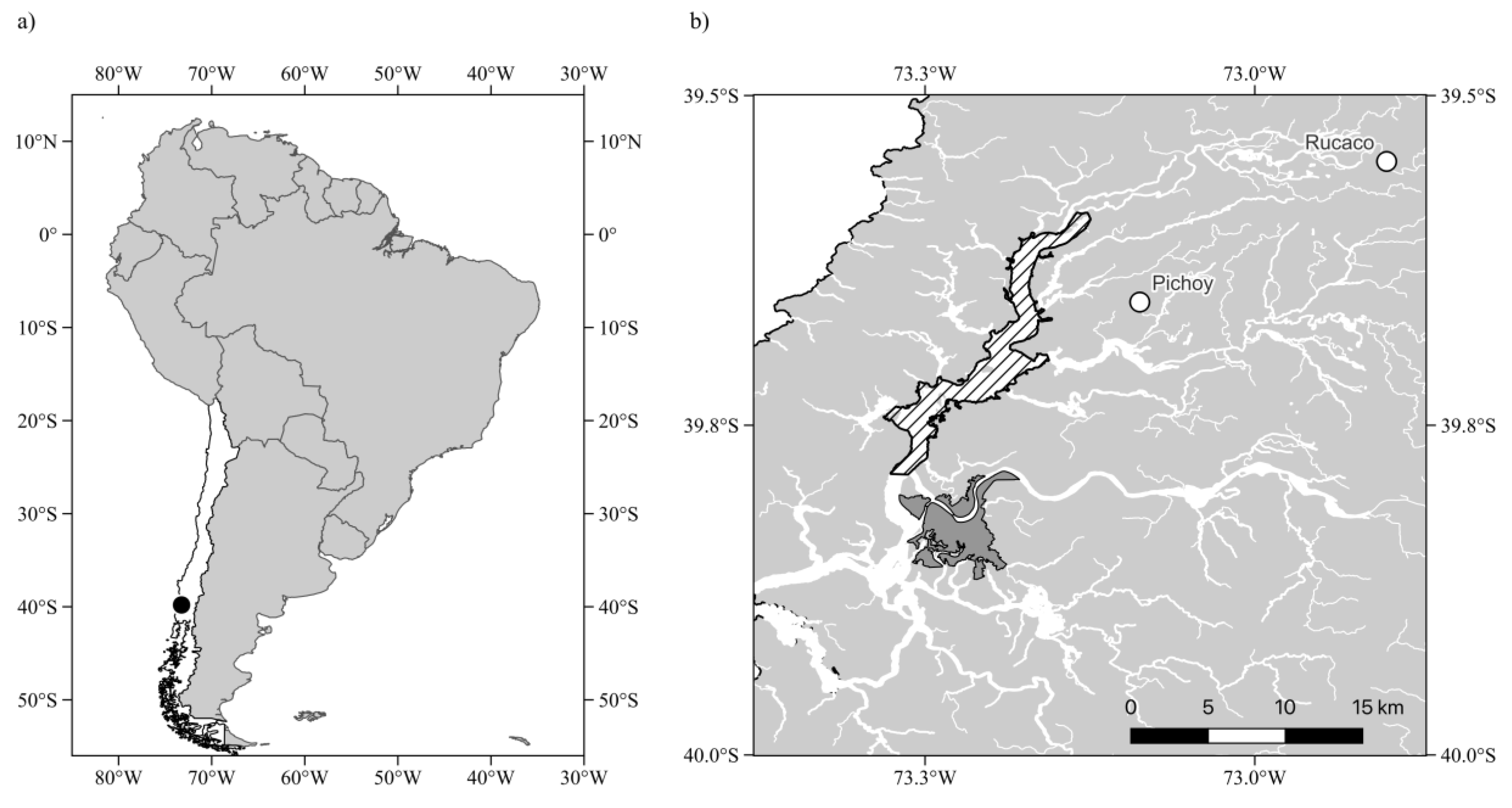
Figure 2.
Assessment of changes in long term patterns in seasonal fluctuations in climatic and hydrologic drivers affecting the RCW. a) average monthly temperature, T (°C), b) monthly cumulative precipitation, P(mm/month), c) average monthly river flow, Flow (m³/s), and d) average monthly water level, Level (m). The continuous black lines show the fit of a cyclic general additive model (GAM) to the seasonal variation across the annual cycle. Data in a) and b) correspond to the weather station at Pichoy Airport (see Figure 1). Data shown in c) and d) correspond to variables measured at Rucaco hydrological station (see Figure 1). The observed variation for the reference baseline period (see Table 1) is represented by black continuous lines, whereas the dashed line indicates the variation observed during the recent decade (2013-2023) and the grey shaded bands show the corresponding 95% confidence intervals for the fitted GAMs.
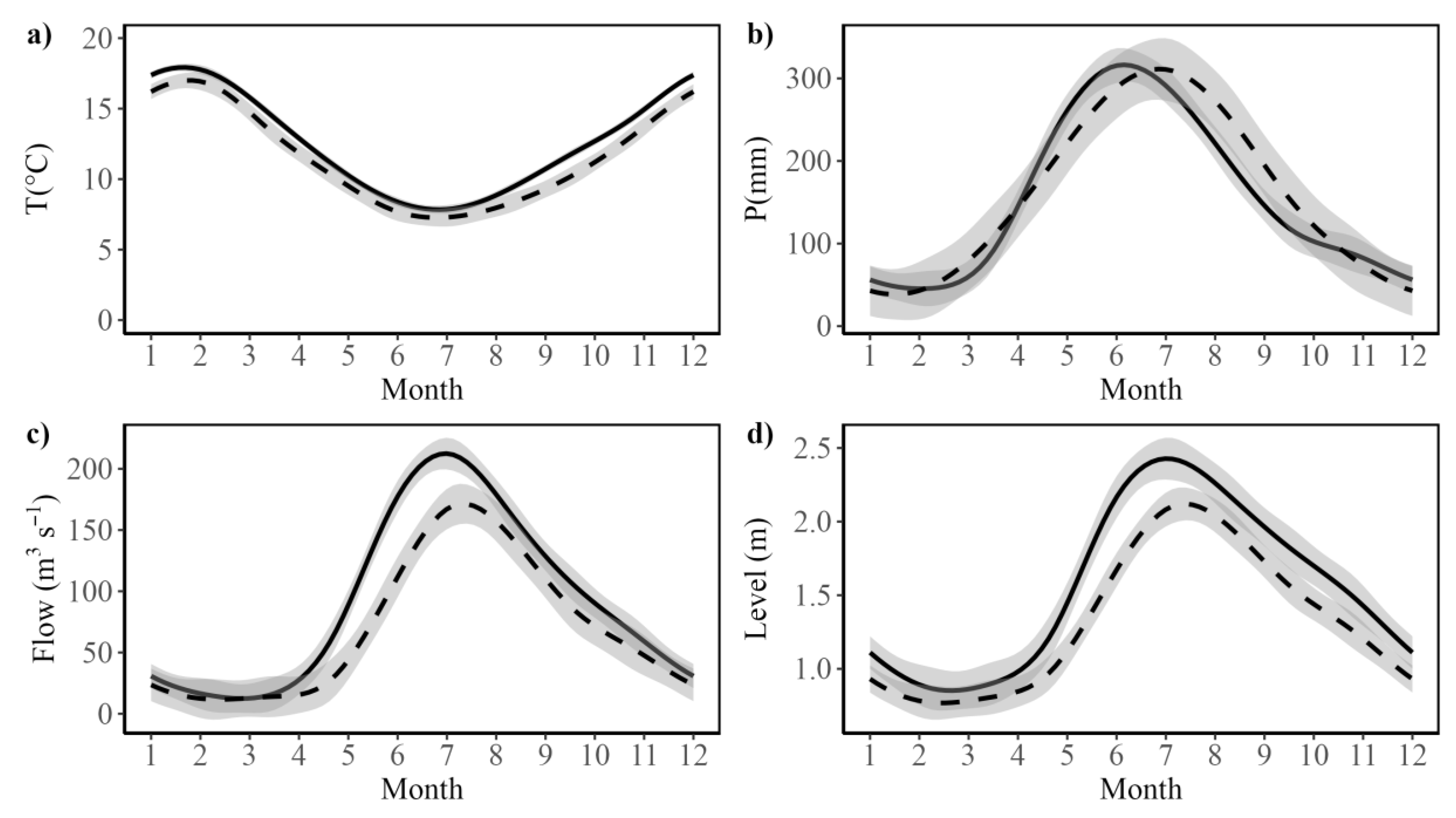
Figure 3.
Spatial time series of SDMs for Egeria densa. The Figure illustrates the data for austral spring-summer seasons in (a) 2015 (b) 2016 (c) 2017 (d) 2018 (e) 2019 (f) 2020 (g) 2021 (h)2022 (i) 2022 and (j) 2023. The Figure shows the estimated presence probability of Egeria densa in each of the modelled pixels, with the color palette ranging from light blue (zero) to red (one), indicating increasingly greater probability of observing Egeria densa (i.e., the estimated habitat suitability index).
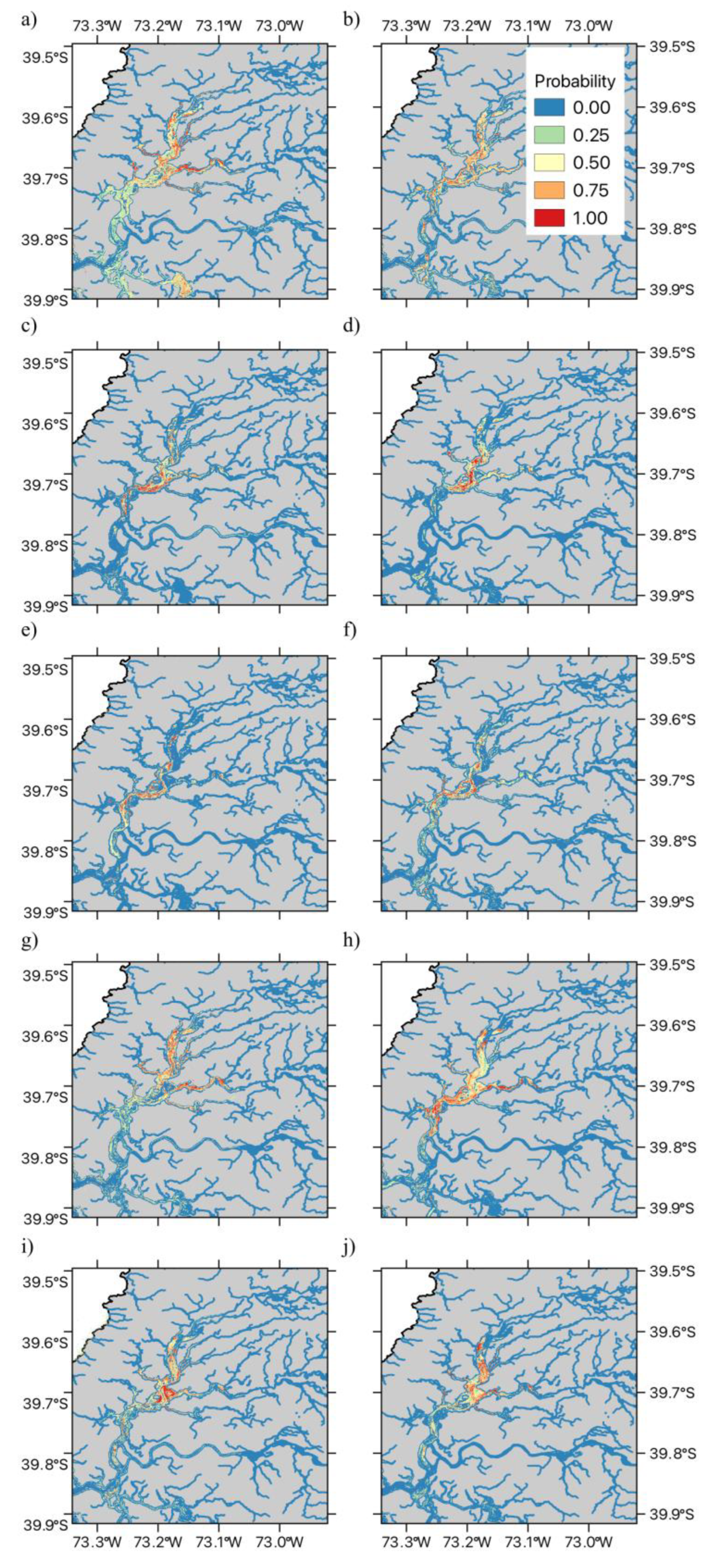
Figure 4.
Spatial time series of SDMs for Schoenoplectus californicus. The Figure illustrates the data for austral spring-summer seasons in (a) 2015 (b) 2016 (c) 2017 (d) 2018 (e) 2019 (f) 2020 (g) 2021 (h)2022 (i) 2022 and (j) 2023. The Figure shows the estimated presence probability of Totora in each of the modelled pixels, with the color palette ranging from light blue (zero) to red (one), indicating increasingly greater probability of observing Schoenoplectus californicus (i.e., the estimated habitat suitability index).
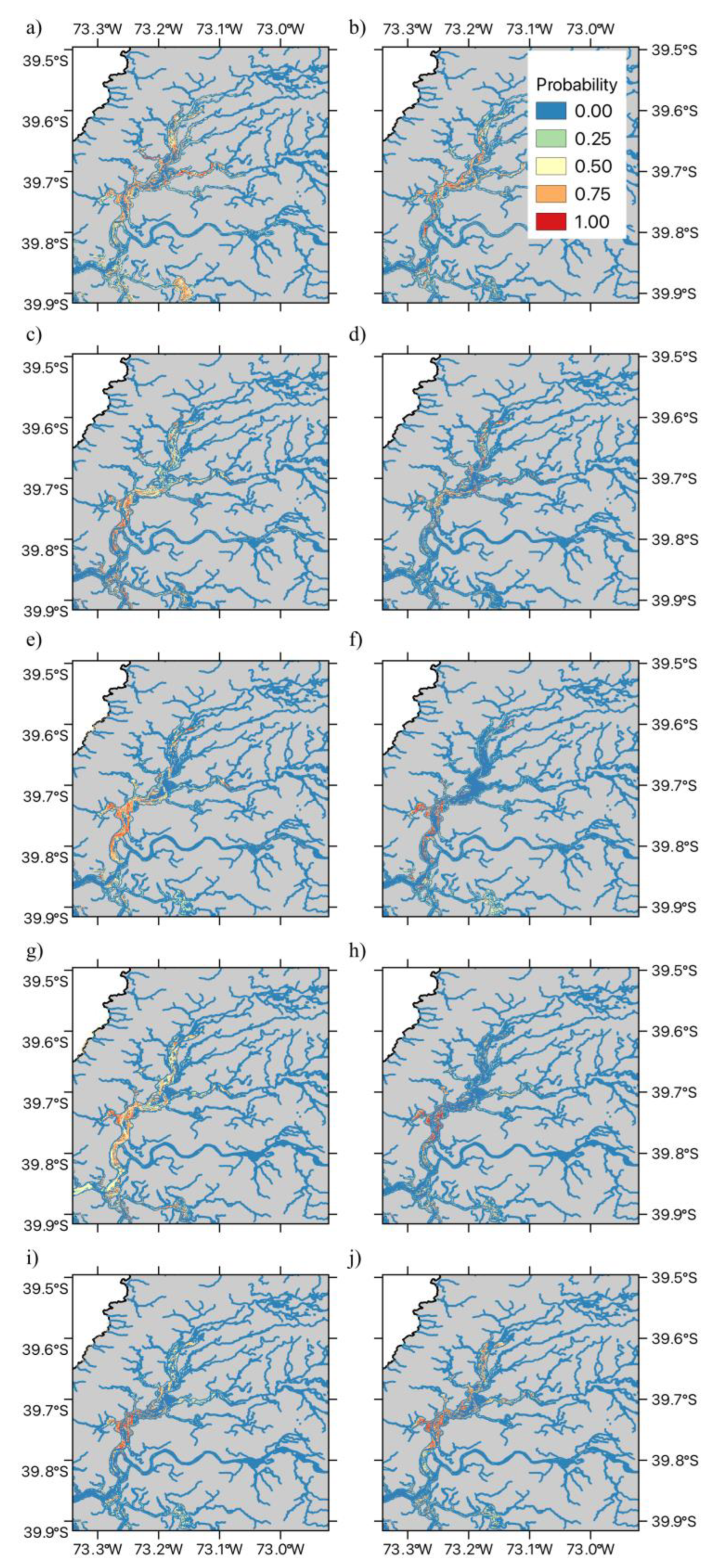
Figure 5.
Temporal variation in the distribution area of the two dominant aquatic macrophyte species within the RCW across the ten years studied. The Figure shows: (a) temporal variation in the area of suitable habitat (measured in km2) for Egeria densa, and (b) temporal variation in the area of suitable habitat (measured in km2) for Schoenoplectus californicus. Dashed lines in figures (a) and (b) show the fitted linear trend, with their confidence intervals are shown in grey.
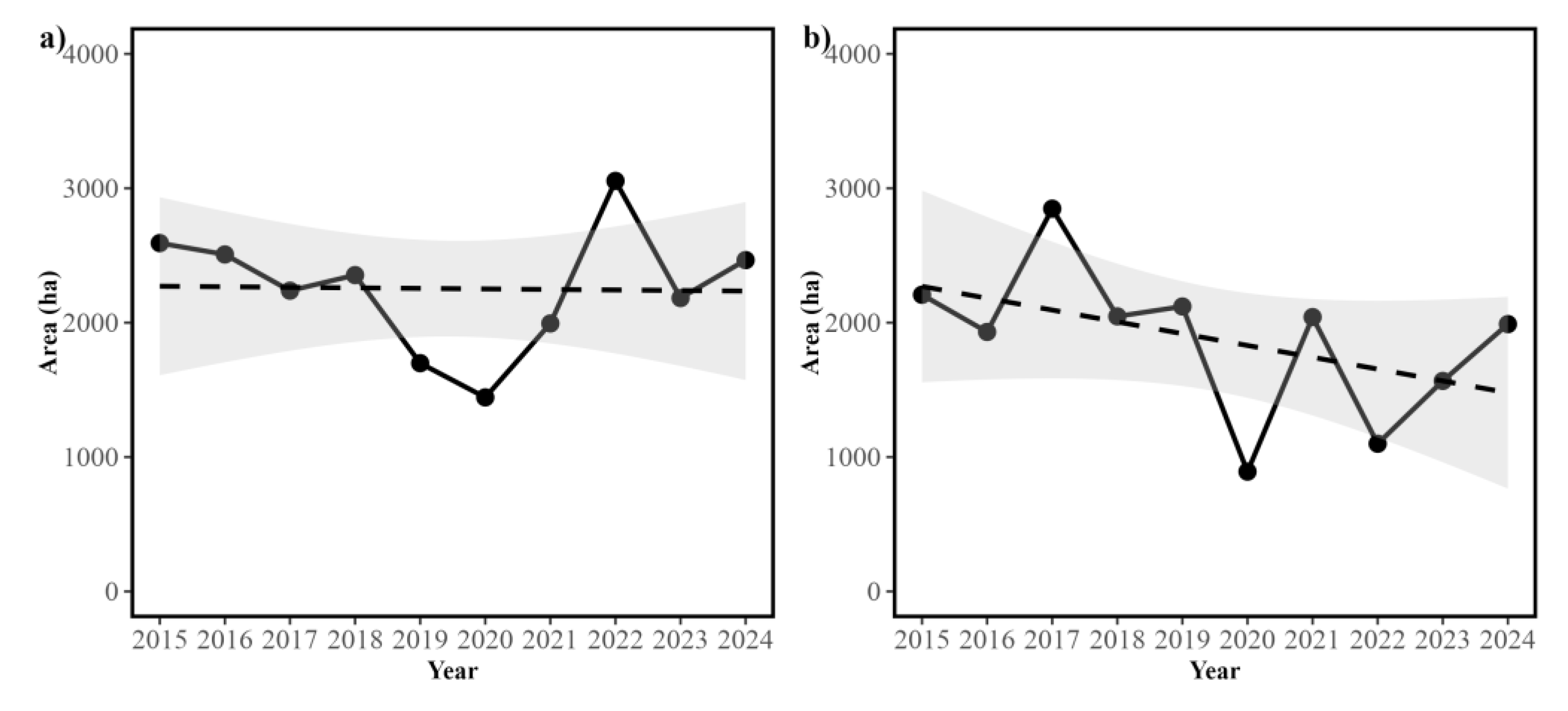

Table 1.
General additive model fit to describe the interdecadal variation in seasonal variability in climatic and hydrological drivers at the RCW. The Table shows average monthly air temperature and precipitation (T (°C) and P (mm) respectively) at Pichoy Airport, as well as the average monthly river flow and water level (Flow (m³/s) and Level (m) respectively) at Rucaco hydrological station. The table shows the estimated parameter values and standard error, as well as the level of significance. The additive effects of the term associated with the intercept (corresponding to the effect of the baseline decades) as well as of the 2013-2023 decade are estimated. The term s(Group) reflects the degree of fit of the nonlinear function adjusted to the seasonal variation over the 12 months of the year. The F statistic and effective degrees of freedom (df) are reported. The level of significance in each estimate is represented according to the following symbols: ns: p ≥ 0.05; *: p < 0.05; **: p < 0.01; ***: p < 0. 001.
| Variable | T(°C) | P(mm) | Flow (m3s-1) | Level (m) |
|---|---|---|---|---|
| Intercept | 13.00±0.06 *** | 153.06±7.40 *** | 88.25±2.11 *** | 1.53±0.02 *** |
| 2013-2023 | -1.01±0.13 *** | 4.36±8.31 ns | -21.69±4.64 *** | -0.23±0.03 *** |
| s(Group) | 6.85 | 5.40 | 6.292 | 6.415 |
| F(df) | 647.7 (8) *** | 100.1 (8) ns | 149.9 (8) *** | 114.5 (8) *** |
| GCV | 1.69 | 7425.90 | 2178.90 | 0.070294 |
| R2adj | 0.89 | 0.55 | 0.70 | 0.80 |
Table 2.
Summary of the Landsat 8 scenes and Maximum Entropy (MaxEnt) SDM statistics for the two dominant aquatic macrophytes at the RCW across the ten years studied. The table shows summary information for (a) Egeria densa and (b) Schoenoplectus californicus. The table shows for each of the ten years the list of Landsat 8 images analyzed to model distribution of these aquatic macrophytes in the study area, indicating the date of the scenes. The table also shows the number of monodominant macrophyte patches with diameter > 30 m (N), as well as the average Area Under the Receiver Operating Characteristic Curve (AUC) value ± 1 standard error for the training and test cross validation sets, as well as the average Maximum test sensitivity plus specificity Cloglog threshold (MSS). This threshold allows the estimation of the occupied versus unoccupied areas of the wetland, by filtering the projected probability maps.
| Year | L8 Scene Date1 |
N | AUC Train | AUC Test | MSS |
|---|---|---|---|---|---|
| a) Egeria densa | |||||
| 2015 | 28/01/2015 | 26 | 0.93 ± 0.005 | 0.89 ± 0.027 | 0.36 ± 0.098 |
| 2016 | 30/12/2015 | 353 | 0.93 ± 0.001 | 0.92 ± 0.003 | 0.35 ± 0.02 |
| 2017 | 30/11/2016 | 46 | 0.97 ± 0.001 | 0.95 ± 0.008 | 0.19 ± 0.029 |
| 2018 | 05/02/2018 | 72 | 0.95 ± 0.002 | 0.94 ± 0.012 | 0.19 ± 0.03 |
| 2019 | 14/01/2019 | 94 | 0.97 ± 0.001 | 0.97 ± 0.003 | 0.23 ± 0.063 |
| 2020 | 11/02/2020 | 37 | 0.96 ± 0.001 | 0.93 ± 0.015 | 0.37 ± 0.071 |
| 2021 | 08/03/2021 | 352 | 0.89 ± 0.001 | 0.88 ± 0.005 | 0.38 ± 0.038 |
| 2022 | 21/12/2021 | 64 | 0.9 ± 0.002 | 0.87 ± 0.016 | 0.3 ± 0.058 |
| 2023 | 03/02/2023 | 37 | 0.93 ± 0.003 | 0.9 ± 0.015 | 0.35 ± 0.022 |
| 2024 | 21/01/2024 | 69 | 0.95 ± 0.001 | 0.93 ± 0.012 | 0.21 ± 0.034 |
| b) Schoenoplectus californicus | |||||
| 2015 | 28/01/2015 | 28 | 0.92 ± 0.002 | 0.89 ± 0.007 | 0.23 ± 0.068 |
| 2016 | 30/12/2015 | 204 | 0.93 ± 0.002 | 0.92 ± 0.007 | 0.3 ± 0.059 |
| 2017 | 30/11/2016 | 18 | 0.95 ± 0.003 | 0.93 ± 0.017 | 0.46 ± 0.11 |
| 2018 | 05/02/2018 | 38 | 0.96 ± 0.001 | 0.94 ± 0.009 | 0.24 ± 0.1 |
| 2019 | 14/01/2019 | 40 | 0.95 ± 0.001 | 0.93 ± 0.008 | 0.35 ± 0.035 |
| 2020 | 11/02/2020 | 50 | 0.96 ± 0.001 | 0.95 ± 0.004 | 0.45 ± 0.099 |
| 2021 | 08/03/2021 | 132 | 0.9 ± 0.002 | 0.89 ± 0.006 | 0.38 ± 0.068 |
| 2022 | 21/12/2021 | 29 | 0.96 ± 0.003 | 0.94 ± 0.012 | 0.44 ± 0.127 |
| 2023 | 03/02/2023 | 309 | 0.92 ± 0.001 | 0.91 ± 0.005 | 0.31 ± 0.029 |
| 2024 | 21/01/2024 | 300 | 0.94 ± 0.001 | 0.93 ± 0.005 | 0.28 ± 0.07 |
1 Scene acquisition dates are shown in format dd/mm/YYYY.
Table 3.
Results of the stepwise linear regression model evaluating the interannual variation in macrophyte area within the RCW as a function of climatic and hydrological variables. The table shows results for a) Egeria densa and b) Schoenoplectus californicus. Selected predictor variables considered include mean annual temperature (TYear (°C), accumulated annual precipitation (sPYear (mm)), mean annual water level ((LevelYear (m)), and annual water level standard deviation (s.d. Level (m)). The table shows fitted regression coefficients with their standard errors (β ± SE), t-Student values, and p-values for each predictor retained in the final model. Model fit statistics, including the adjusted R² and overall model significance, are also reported. The level of significance in each estimate is represented according to the following symbols: ns: p ≥ 0.05; *: p < 0.05; **: p < 0.01; ***: p < 0. 001. bold.
| Species and Variables |
β ± SE | t | p-Value |
|---|---|---|---|
| a) Egeria densa | |||
| Intercept | -3733.32 ± 1157.59 | -3.23 | 0.018*** |
| Year | 1.83 ± 0.57 | 3.22 | 0.018*** |
| TYear (°C) | 6.93 ± 1.72 | 4.02 | 0.007*** |
| s.d. Level (m) | -32.94 ± 11.76 | -2.80 | 0.031** |
| b) Schoenoplectus californicus | |||
| Intercept | 3072 ± 1395 | 2.20 | 0.093ns |
| Year | -1.46 ± 0.68 | -2.15 | 0.098 ns |
| T (°C) | -6.19 ± 1.85 | -3.35 | 0.029** |
| sPYear (mm) | 0.02 ± 0.003 | 5.13 | 0.007*** |
| Level (m) | -46.47 ± 9.99 | -4.65 | 0.010** |
| s.d. Level (m) | 14.95 ± 12.38 | 1.20 | 0.294 ns |
Disclaimer/Publisher’s Note: The statements, opinions and data contained in all publications are solely those of the individual author(s) and contributor(s) and not of MDPI and/or the editor(s). MDPI and/or the editor(s) disclaim responsibility for any injury to people or property resulting from any ideas, methods, instructions or products referred to in the content. |
© 2025 by the authors. Licensee MDPI, Basel, Switzerland. This article is an open access article distributed under the terms and conditions of the Creative Commons Attribution (CC BY) license (http://creativecommons.org/licenses/by/4.0/).
Copyright: This open access article is published under a Creative Commons CC BY 4.0 license, which permit the free download, distribution, and reuse, provided that the author and preprint are cited in any reuse.


