Electrical and Magnetic Interactions as Manifestations of 5-Dimensional Space Geometry and Vacuum Energy Density Dynamics

1. Introduction

Electromagnetic and gravitational forces are among the most fundamental interactions in physics. These forces govern the behavior of matter and energy on scales ranging from subatomic particles to cosmological structures. Despite extensive empirical data and theoretical models describing their behavior, the true nature and material essence from which they arise remain subjects of intensive research.

From a physical standpoint, we understand how these forces act and can predict their effects with high accuracy. However, fundamental questions remain: What exactly are these forces? How are they interconnected? And, most importantly, what is the nature of protomatter - the fundamental substance from which these forces emerge? These questions lie not only in the realm of physical principles but also touch upon philosophical aspects of the nature of reality.

This article proposes a theoretical model introducing an additional spatial dimension called "space density". We hypothesize that this dimension plays a key role in the formation of gravitational and electromagnetic fields. Our model indicates that traditional three-dimensional space combined with time is insufficient for a complete explanation of the origin of these forces. Instead, space itself may possess intrinsic properties that facilitate the formation of these fields. By expanding our understanding of space through the inclusion of an additional dimension, we explore the possibility of new interpretations of gravitational and electromagnetic interactions. In the course of this research, we will conclude that the stated problem within the formulated postulates has no solution in three-dimensional space, since a violation of the postulate of conservation of space density quantity is discovered. As a result, we will be forced to transition to consideration of 5D-space, formed from two orthogonal 3D-subspaces with one common axis.

2. Hypothesis

We propose that electromagnetic and gravitational fields are manifestations of a more fundamental property of space, which can be interpreted as "space density". This property defines a quantitative characteristic of space, while being conceptually distinct from matter density. This quantity, unlike matter density, is continuous - just as time and the three spatial coordinates are continuous. Furthermore, unlike baryonic matter, space density, if considered as matter, does not cause curvature of the space metric, meaning it possesses no mass, inertia, friction, or viscosity. It is a certain idealized matter that, in its tendency towards maximum entropy, can manifest in interactions caused by distribution inhomogeneity, which we interpret as the curvature of space itself without curvature of its metric.

In this model, "space density" represents a measure of how space itself can be compressed or expanded independently of its metric. This density is not analogous to matter density in three-dimensional space, but rather reflects a fundamental characteristic of space influencing field formation.

Our hypothesis is based on several key postulates:

• Space Density: In five-dimensional space, the density $\rho \left(r\right)$ characterizes the state of space and can change, thereby allowing us to speak of space curvature without curvature of its metric. Let us call this phenomenon first-order space curvature. A similar term is used in relativity theory, but within our theory it will have a somewhat different context.
• Spherical Symmetry of Perturbations: The distribution of space density $\rho \left(r\right)$ during its perturbation is assumed to be spherically symmetric relative to the perturbation center.
• Conservation of Space Density Quantity: Upon perturbation in some region of space, the surrounding space is capable of changing its density such that the total "density" of space over an infinite volume remains unchanged. In other words, in a certain approximation, the total quantity of space density is conserved.
• Postulate of Maximum Entropy of Space Density Distribution: Space tends towards a state of maximum entropy, i.e., a uniform density distribution. This principle defines the natural tendency of space to return to a uniform density distribution after perturbations, analogous to thermodynamic principles governing physical systems.

By exploring these postulates within the framework of 5D-space, we aim to provide a deeper understanding of the origin of electromagnetic fields. This model challenges the traditional view of the independence of these fields and instead suggests they are interconnected through the intrinsic properties of space itself. In the course of this research, we will obtain a completely unexpected result: Coulomb’s law, containing a correction for the interaction of elementary charges at distances comparable to their "classical" physical sizes (this phenomenon is well-studied in QED - screening).

3. Methodology

3.1. Distribution of Space Density Around a Single Compressed Spherical Region of Space

We consider two states of the universe: in the first state, the density throughout space is ${\rho }_0$ and is some constant. In the second system state, we have a certain region of space bounded by a sphere $S\left(R_1\right)$, which we compress to $S\left(R_1^{\prime }\right)$. We need to find the distribution of space density inside the sphere and outside it, based on the laws we have established operating in our hypothetical universe.

3.1.1. Density Distribution After Compression

The density after compression inside the sphere is defined as ${\rho }_{\mathrm{inside}}={\rho }_0+{\rho }_1$, where ${\rho }_1$ is the added density, determined from the ratio of volumes before and after compression:

$${\rho }_{0}V\left(R_1\right)={\rho }_{\mathrm{inside}}V\left(R_1^{\prime }\right)$$

Substitute the sphere volumes:

$${\rho }_0{\displaystyle \frac{4}{3}}\pi R_1^3=({\rho }_0+{\rho }_1){\displaystyle \frac{4}{3}}\pi R_1^{\prime 3}$$

Simplify:

$${\rho }_0{R}_1^3=({\rho }_0+{\rho }_1)R_1^{\prime 3}$$

$${\rho }_1={\rho }_0\left({\displaystyle \frac{R_1^3}{R_1^{\prime 3}}}-1\right)$$

3.1.2. Density Distribution Outside the Sphere

We proceed from the assumption that outside the sphere, the amount of removed space density must equal the amount added inside it, ${\rho }_1·V\left(R_1^{\prime }\right)$. Therefore, when integrating the perturbation from the surface of the compressed sphere to infinity, the integral must yield a finite number, i.e., converge, and accordingly the integrand must be convergent. In three-dimensional space, such a function is $1/r^4$. Assume that the distribution of reduced density outside the compressed region of space will satisfy this dependence on distances from the perturbation center. Then we obtain the following dependence for the space density distribution outside the compressed sphere:

$$\Delta {\rho }_{\mathrm{decrease}}\left(r\right)={\displaystyle \frac{A}{r^4}}$$

3.1.3. Normalization Coefficient A

To satisfy the law of conservation of space density, the integral of $\Delta {\rho }_{\mathrm{decrease}}\left(r\right)$ over the volume from $R_1^{\prime }$ to infinity must equal the added density inside the sphere:

$${\rho }_{1}V\left(R_1^{\prime }\right)={\int }_{R_1^{\prime }}^{\infty }\Delta {\rho }_{\mathrm{decrease}}\left(r\right)·dV$$

Or, taking into account the law of spherical symmetry, in the spherical coordinate system the integral simplifies to:

$${\rho }_{1}V\left(R_1^{\prime }\right)={\int }_{R_1^{\prime }}^{\infty }\Delta {\rho }_{\mathrm{decrease}}\left(r\right)·4\pi r^{2}dr$$

Substitute:

$${\rho }_1{\displaystyle \frac{4}{3}}\pi R_1^{\prime 3}=4\pi {\int }_{R_1^{\prime }}^{\infty }{\displaystyle \frac{A}{r^4}}{r}^{2}dr$$

Solve the integral:

$$4\pi A{\int }_{R_1^{\prime }}^{\infty }{\displaystyle \frac{1}{r^2}}dr=4\pi A{\left[-{\displaystyle \frac{1}{r}}\right]}_{R_1^{\prime }}^{\infty }=4\pi A\left({\displaystyle \frac{1}{R_1^{\prime }}}-0\right)={\displaystyle \frac{4\pi A}{R_1^{\prime }}}$$

Equality of density quantities:

$${\rho }_1{\displaystyle \frac{4}{3}}\pi R_1^{\prime 3}={\displaystyle \frac{4\pi A}{R_1^{\prime }}}$$

Find A:

$$A={\rho }_1{\displaystyle \frac{R_1^{\prime 4}}{3}}$$

Final formula for $\Delta {\rho }_{\mathrm{decrease}}\left(r\right)$:

$$\Delta {\rho }_{\mathrm{decrease}}\left(r\right)={\displaystyle \frac{A}{r^4}}={\displaystyle \frac{{\rho }_1\frac{R_1^{\prime 4}}{3}}{r^4}}$$

Now multiply numerator and denominator by $4\pi$:

$$\Delta {\rho }_{\mathrm{decrease}}\left(r\right)={\displaystyle \frac{4\pi {\rho }_1\frac{R_1^{\prime 4}}{3}}{4\pi r^4}}={\displaystyle \frac{{\rho }_1\frac{4}{3}\pi R_1^{\prime 4}}{4\pi r^4}}={\displaystyle \frac{{\rho }_1·R_1^{\prime }·V\left(R_1^{\prime }\right)}{4\pi r^4}}$$

Thus we have obtained the following formula for the density distribution outside the sphere $\Delta {\rho }_{\mathrm{decrease}}\left(r\right)$:

$$\Delta {\rho }_{\mathrm{decrease}}\left(r\right)={\displaystyle \frac{{\rho }_1·R_1^{\prime }·V\left(R_1^{\prime }\right)}{4\pi r^4}}$$

(1)

Also taking into account that the amount of added density in the volume of the compressed sphere is expressed by the formula:

$$Q=\left(V\left(R_1\right)-V\left(R_1^{\prime }\right)\right)·{\rho }_0$$

where $V\left(R_1\right)$ and $V\left(R_1^{\prime }\right)$ are the volumes of spheres with radii $R_1$ and $R_1^{\prime }$ respectively. And also taking into account the formula for ${\rho }_1$ - the density of the amount of added density inside the sphere:

$${\rho }_1={\displaystyle \frac{Q}{V\left(R_1^{\prime }\right)}}$$

where $V\left(R_1^{\prime }\right)$ is the volume of the sphere after compression.

We can express the obtained formula for the space density distribution $\Delta {\rho }_{\mathrm{decrease}}\left(r\right)$ as:

$$\Delta {\rho }_{\mathrm{decrease}}\left(r\right)={\displaystyle \frac{Q·R_1^{\prime }}{4\pi r^4}}$$

(2)

Where Q is the amount of density added to the volume of sphere $S\left(R_1^{\prime }\right)$, $R_1^{\prime }$ is the radius of the compressed sphere, and r is the distance from the center of the sphere to a point in space in the spherical coordinate system.

3.1.4. Verification of Conservation of Space Density Quantity

For the fulfillment of the third law established in our system, the following equality must hold:

$${\int }_{R_1^{\prime }}^{\infty }\Delta {\rho }_{\mathrm{decrease}}\left(r\right)·dV={\int }_{R_1^{\prime }}^{\infty }\Delta {\rho }_{\mathrm{decrease}}\left(r\right)·4\pi r^{2}dr={\rho }_{1}V\left(R_1^{\prime }\right)$$

Substitute the expression for $\Delta {\rho }_{\mathrm{decrease}}\left(r\right)$:

$${\int }_{R_1^{\prime }}^{\infty }{\displaystyle \frac{{\rho }_1·R_1^{\prime }·V\left(R_1^{\prime }\right)}{4\pi r^4}}·4\pi r^{2}dr={\rho }_1·R_1^{\prime }·V\left(R_1^{\prime }\right){\int }_{R_1^{\prime }}^{\infty }{\displaystyle \frac{1}{r^2}}dr$$

Integrate and substitute the integration limits:

$${\rho }_1·R_1^{\prime }·V\left(R_1^{\prime }\right){\left[-{\displaystyle \frac{1}{r}}\right]}_{R_1^{\prime }}^{\infty }={\rho }_1·R_1^{\prime }·V\left(R_1^{\prime }\right)\left({\displaystyle \frac{1}{R_1^{\prime }}}-0\right)={\displaystyle \frac{{\rho }_1·R_1^{\prime }·V\left(R_1^{\prime }\right)}{R_1^{\prime }}}$$

We obtain:

$${\int }_{R_1^{\prime }}^{\infty }\Delta {\rho }_{\mathrm{decrease}}\left(r\right)·dV={\rho }_{1}V\left(R_1^{\prime }\right)={\rho }_1{\displaystyle \frac{4}{3}}\pi R_1^{\prime 3}$$

Thus we have verified that our distribution of space density outside the compressed sphere, proportional to $1/r^4$, is consistent with our third law of conservation of space density in the system, taking into account the normalization coefficient A.

4. Expression for the Complete Distribution of Space Density for a Single Compressed Sphere

Let us write our distribution taking into account boundary conditions using the Heaviside function. This representation of the space density distribution will be needed to find the total interaction quantity of two density clusters, considering the space density added to the first cluster, as well as the gradient at the transition boundary—the sphere bounding the first cluster. Why this is important will become clear in the next section of my article.

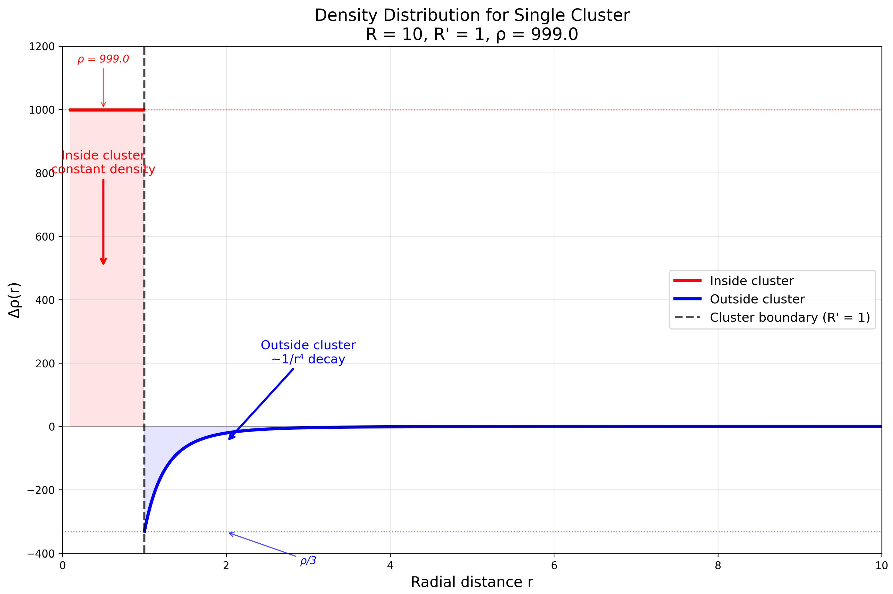
Figure 1. Graphs of space density distribution along a line passing through the center of the compressed sphere

Figure 1. Graphs of space density distribution along a line passing through the center of the compressed sphere

4.1. Representation of Space Density Distribution Using the Heaviside Function

The space density distribution, $\rho \left(r\right)$, for a single sphere can be expressed using the Heaviside function $H\left(x\right)$ for an accurate description of the density inside and outside the compressed sphere. The main density distribution is defined as:

$$\rho \left(r\right)=\left\{\begin{array}{cc}{\rho }_0+{\rho }_1,\hfill & \mathrm{if}r\le R_1^{\prime }\hfill \\ {\rho }_0-{\displaystyle \frac{R_1^{\prime }·{\rho }_1·V\left(R_1^{\prime }\right)}{4\pi r^4}},\hfill & \mathrm{if}r>R_1^{\prime }\hfill \end{array}\right.$$

The density increase $\Delta {\rho }_{\mathrm{increase}}\left(r\right)$ inside the compressed region can be expressed as:

$$\Delta {\rho }_{\mathrm{increase}}\left(r\right)=\left\{\begin{array}{cc}{\rho }_1,\hfill & \mathrm{if}r\le R_1^{\prime }\hfill \\ 0,\hfill & \mathrm{if}r>R_1^{\prime }\hfill \end{array}\right.$$

Similarly, the density decrease $\Delta {\rho }_{\mathrm{decrease}}\left(r\right)$ outside the sphere:

$$\Delta {\rho }_{\mathrm{decrease}}\left(r\right)=\left\{\begin{array}{cc}0,\hfill & \mathrm{if}r\le R_1^{\prime }\hfill \\ {\displaystyle \frac{R_1^{\prime }·{\rho }_1·V\left(R_1^{\prime }\right)}{4\pi r^4}},\hfill & \mathrm{if}r>R_1^{\prime }\hfill \end{array}\right.$$

We can now rewrite these expressions in terms of the Heaviside function $H\left(x\right)$:

$$\Delta {\rho }_{\mathrm{increase}}\left(r\right)={\rho }_{1}H(R_1^{\prime }-r)$$

$$\Delta {\rho }_{\mathrm{decrease}}\left(r\right)={\displaystyle \frac{R_1^{\prime }·{\rho }_1·V\left(R_1^{\prime }\right)}{4\pi r^4}}H(r-R_1^{\prime })$$

Thus, the total density change $\Delta \rho \left(r\right)$ is:

$$\Delta \rho \left(r\right)={\rho }_{1}H(R_1^{\prime }-r)-{\displaystyle \frac{R_1^{\prime }·{\rho }_1·V\left(R_1^{\prime }\right)}{4\pi r^4}}H(r-R_1^{\prime })$$

4.1.1. Boundary Conditions Check

Now let us verify the boundary conditions:

1. For $r\le R_1^{\prime }$:

$$\Delta \rho \left(r\right)={\rho }_{1}H(R_1^{\prime }-r)-{\displaystyle \frac{R_1^{\prime }·{\rho }_1·V_{R{1}^{\prime }}}{4\pi r^4}}H(r-R_1^{\prime })$$

Since $H(R_1^{\prime }-r)=1$ and $H(r-R_1^{\prime })=0$:

$$\Delta \rho \left(r\right)={\rho }_1-0={\rho }_1$$

2. For $r>R_1^{\prime }$:

$$\Delta \rho \left(r\right)={\rho }_{1}H(R_1^{\prime }-r)-{\displaystyle \frac{R_1^{\prime }·{\rho }_1·V_{R{1}^{\prime }}}{4\pi r^4}}H(r-R_1^{\prime })$$

Since $H(R_1^{\prime }-r)=0$ and $H(r-R_1^{\prime })=1$:

$$\Delta \rho \left(r\right)=0-{\displaystyle \frac{R_1^{\prime }·{\rho }_1·V_{R{1}^{\prime }}}{4\pi r^4}}$$

Now substitute $V_{R{1}^{\prime }}={\displaystyle \frac{4}{3}}\pi {\left(R_1^{\prime }\right)}^3$:

$$\Delta \rho \left(r\right)=-{\displaystyle \frac{R_1^{\prime }·{\rho }_1·\frac{4}{3}\pi {\left(R_1^{\prime }\right)}^3}{4\pi r^4}}=-{\displaystyle \frac{{\rho }_1·R_1^{\prime 4}}{3r^4}}$$

Thus, we arrive at the following expression for $\Delta \rho \left(r\right)$ in terms of the Heaviside function:

$$\Delta \rho \left(r\right)={\rho }_{1}H(R_1^{\prime }-r)-{\displaystyle \frac{{\rho }_1·R_1^{\prime 4}}{3r^4}}H(r-R_1^{\prime })$$

(3)

4.2. Verification of the Space Density Conservation Condition

To verify, let us take the integral of $\Delta \rho \left(r\right)$. Let us integrate $\Delta \rho \left(r\right)$ over the entire volume. Recall that $\Delta \rho \left(r\right)$ is represented as:

$$\Delta \rho \left(r\right)={\rho }_1\left[H(R_1^{\prime }-r)-{\displaystyle \frac{R_1^{\prime 4}}{3r^4}}H(r-R_1^{\prime })\right]$$

Compute the integral:

$${\int }_0^{\infty }\Delta \rho \left(r\right)·4\pi r^{2}dr$$

Split the integral into two parts corresponding to $\Delta {\rho }_{\mathrm{increase}}\left(r\right)$ and $\Delta {\rho }_{\mathrm{decrease}}\left(r\right)$:

$${\int }_0^{\infty }\Delta \rho \left(r\right)·4\pi r^{2}dr={\int }_0^{\infty }\left[{\rho }_{1}H(R_1^{\prime }-r)-{\displaystyle \frac{{\rho }_1·R_1^{\prime 4}}{3r^4}}H(r-R_1^{\prime })\right]·4\pi r^{2}dr$$

Split into two separate integrals:

$${\int }_0^{\infty }{\rho }_{1}H(R_1^{\prime }-r)·4\pi r^{2}dr-{\int }_0^{\infty }{\displaystyle \frac{{\rho }_1·R_1^{\prime 4}}{3r^4}}H(r-R_1^{\prime })·4\pi r^{2}dr$$

Consider the first integral:

$${\int }_0^{R_1^{\prime }}{\rho }_1·4\pi r^{2}dr=4\pi {\rho }_1{\int }_0^{R_1^{\prime }}{r}^{2}dr=4\pi {\rho }_1{\left[{\displaystyle \frac{r^3}{3}}\right]}_0^{R_1^{\prime }}=4\pi {\rho }_1·{\displaystyle \frac{{\left(R_1^{\prime }\right)}^3}{3}}={\displaystyle \frac{4\pi {\rho }_1{\left(R_1^{\prime }\right)}^3}{3}}$$

Now consider the second integral:

$${\int }_{R_1^{\prime }}^{\infty }{\displaystyle \frac{{\rho }_1·R_1^{\prime 4}}{3r^4}}·4\pi r^{2}dr={\displaystyle \frac{4\pi {\rho }_1{R}_1^{\prime 4}}{3}}{\int }_{R_1^{\prime }}^{\infty }{\displaystyle \frac{1}{r^2}}dr={\displaystyle \frac{4\pi {\rho }_1{R}_1^{\prime 4}}{3}}{\left[-{\displaystyle \frac{1}{r}}\right]}_{R_1^{\prime }}^{\infty }$$

Evaluate the limits:

$${\displaystyle \frac{4\pi {\rho }_1{R}_1^{\prime 4}}{3}}\left(-{\displaystyle \frac{1}{\infty }}+{\displaystyle \frac{1}{R_1^{\prime }}}\right)={\displaystyle \frac{4\pi {\rho }_1{R}_1^{\prime 4}}{3}}·{\displaystyle \frac{1}{R_1^{\prime }}}={\displaystyle \frac{4\pi {\rho }_1{R}_1^{\prime 3}}{3}}$$

Now add both results:

$${\int }_0^{\infty }\Delta \rho \left(r\right)·4\pi r^{2}dr={\displaystyle \frac{4\pi {\rho }_1{\left(R_1^{\prime }\right)}^3}{3}}-{\displaystyle \frac{4\pi {\rho }_1{\left(R_1^{\prime }\right)}^3}{3}}=0$$

Thus, the integral of $\Delta \rho \left(r\right)$ over the entire volume is zero:

$${\int }_0^{\infty }\Delta \rho \left(r\right)·4\pi r^{2}dr=0$$

We obtained the predictable result, but this was necessary for verification.

5. Perturbation Quantity (Interaction Quantity) of Two Compressed Spheres of Space Density

5.1. Complete Density Distribution via Heaviside Functions

5.1.1. For a Single Cluster

For a single cluster of space density, the perturbation distribution relative to the radial distance $r_1$ is given by the expression:

$$\Delta {\rho }_1\left({\mathbf{r}}_1\right)={\rho }_{1}H(R_1^{\prime }-r_1)-{\displaystyle \frac{{\rho }_1{R}_1^{\prime 4}}{3r_1^4}}H(r_1-R_1^{\prime }),$$

where:

• ${\rho }_1$ is the amplitude of the density perturbation of the cluster;
• $R_1^{\prime }$ is the radius of the deformed region of space;
• $H\left(x\right)$ is the Heaviside function, ensuring the separation of internal and external regions.

5.1.2. For Two Clusters via Curvature Coefficients

Curvature Coefficient for the First Cluster

$$K_1\left({\mathbf{r}}_1\right)=1+{\displaystyle \frac{\Delta {\rho }_1\left({\mathbf{r}}_1\right)}{{\rho }_0}}=1+{\displaystyle \frac{1}{{\rho }_0}}\left[{\rho }_{1}H(R_1^{\prime }-r_1)-{\displaystyle \frac{{\rho }_1{R}_1^{\prime 4}}{3r_1^4}}H(r_1-R_1^{\prime })\right]$$

Curvature Coefficient for the Second Cluster

$$\begin{array}{c}{K}_2\left({\mathbf{r}}_1\right)=1+{\displaystyle \frac{\Delta {\rho }_2({\mathbf{r}}_1-\mathbf{D})}{{\rho }_0}}\hfill \\ \hfill =1+{\displaystyle \frac{1}{{\rho }_0}}\left[{\rho }_{2}H(R_2^{\prime }-|{\mathbf{r}}_1-\mathbf{D}\left|\right)-{\displaystyle \frac{{\rho }_2{R}_2^{\prime 4}}{3|{\mathbf{r}}_1{-\mathbf{D}|}^4}}H\left(\right|{\mathbf{r}}_1-\mathbf{D}|-R_2^{\prime })\right],\end{array}$$

where $\mathbf{D}$ is the vector displacement of the center of the second cluster relative to the first.

5.1.3. Total Curvature Coefficient and Complete Density Change

If the curvature coefficient of space density is understood as its stretching or compression coefficient, then when superimposing curvature regions from different clusters (beyond their boundaries), it is obvious that the coefficients will multiply. This is equivalent to stretching what is already stretched; accordingly, the total curvature coefficient of space created by two clusters is determined by the product of their individual coefficients:

$$K_{\mathrm{total}}\left({\mathbf{r}}_1\right)=K_1\left({\mathbf{r}}_1\right)·K_2\left({\mathbf{r}}_1\right).$$

(4)

Correspondingly, the total perturbation of space density takes the form:

$$\begin{array}{cc}\Delta {\rho }_{\mathrm{total}}\left({\mathbf{r}}_1\right)={\rho }_0\left[K_{\mathrm{total}}\left({\mathbf{r}}_1\right)-1\right]\hfill & \\ & \hfill ={\rho }_0\left[\left(1+{\displaystyle \frac{\Delta {\rho }_1\left({\mathbf{r}}_1\right)}{{\rho }_0}}\right)\left(1+{\displaystyle \frac{\Delta {\rho }_2({\mathbf{r}}_1-\mathbf{D})}{{\rho }_0}}\right)-1\right].\end{array}$$

Or, expanding the expression:

$$\Delta {\rho }_{\mathrm{total}}\left({\mathbf{r}}_1\right)=\Delta {\rho }_1\left({\mathbf{r}}_1\right)+\Delta {\rho }_2({\mathbf{r}}_1-\mathbf{D})+{\displaystyle \frac{\Delta {\rho }_1\left({\mathbf{r}}_1\right)\Delta {\rho }_2({\mathbf{r}}_1-\mathbf{D})}{{\rho }_0}}.$$

The third (nonlinear) term reflects the mutual violation of the uniform distribution of space density, arising from the superposition of curvatures of both clusters. It is this term that is responsible for the quantity of space density perturbation in the case of two clusters of this density at distance D.

The complete form with Heaviside functions, which we will use for integration, is defined by the formula:

$$\begin{array}{c}\Delta {\rho }_{\mathrm{total}}\left({\mathbf{r}}_1\right)={\rho }_{1}H(R_1^{\prime }-r_1)-{\displaystyle \frac{{\rho }_1{R}_1^{\prime 4}}{3r_1^4}}H(r_1-R_1^{\prime })\hfill \\ \hspace{1em}\hspace{1em}\hspace{1em}\hspace{1em}\hspace{1em}\hspace{1em}\hspace{1em}\hspace{1em}+{\rho }_{2}H(R_2^{\prime }-|{\mathbf{r}}_1-\mathbf{D}\left|\right)-{\displaystyle \frac{{\rho }_2{R}_2^{\prime 4}}{3|{\mathbf{r}}_1{-\mathbf{D}|}^4}}H\left(\right|{\mathbf{r}}_1-\mathbf{D}|-R_2^{\prime })\hfill \\ \hspace{1em}\hspace{1em}\hspace{1em}\hspace{1em}\hspace{1em}\hspace{1em}\hspace{1em}\hspace{1em}\hspace{1em}\hspace{1em}+{\displaystyle \frac{1}{{\rho }_0}}\left[{\rho }_{1}H(R_1^{\prime }-r_1)-{\displaystyle \frac{{\rho }_1{R}_1^{\prime 4}}{3r_1^4}}H(r_1-R_1^{\prime })\right]\hfill \\ \hspace{1em}\hspace{1em}\hspace{1em}\hspace{1em}\hspace{1em}\hspace{1em}\hspace{1em}\hspace{1em}\hspace{1em}\hspace{1em}\hspace{1em}\hspace{1em}\hspace{1em}\hspace{1em}\times \left[{\rho }_{2}H(R_2^{\prime }-|{\mathbf{r}}_1-\mathbf{D}\left|\right)-{\displaystyle \frac{{\rho }_2{R}_2^{\prime 4}}{3|{\mathbf{r}}_1{-\mathbf{D}|}^4}}H\left(\right|{\mathbf{r}}_1-\mathbf{D}|-R_2^{\prime })\right].\hfill \end{array}$$

(5)

Figure 2. Visualization of the space density distribution for two spherical clusters

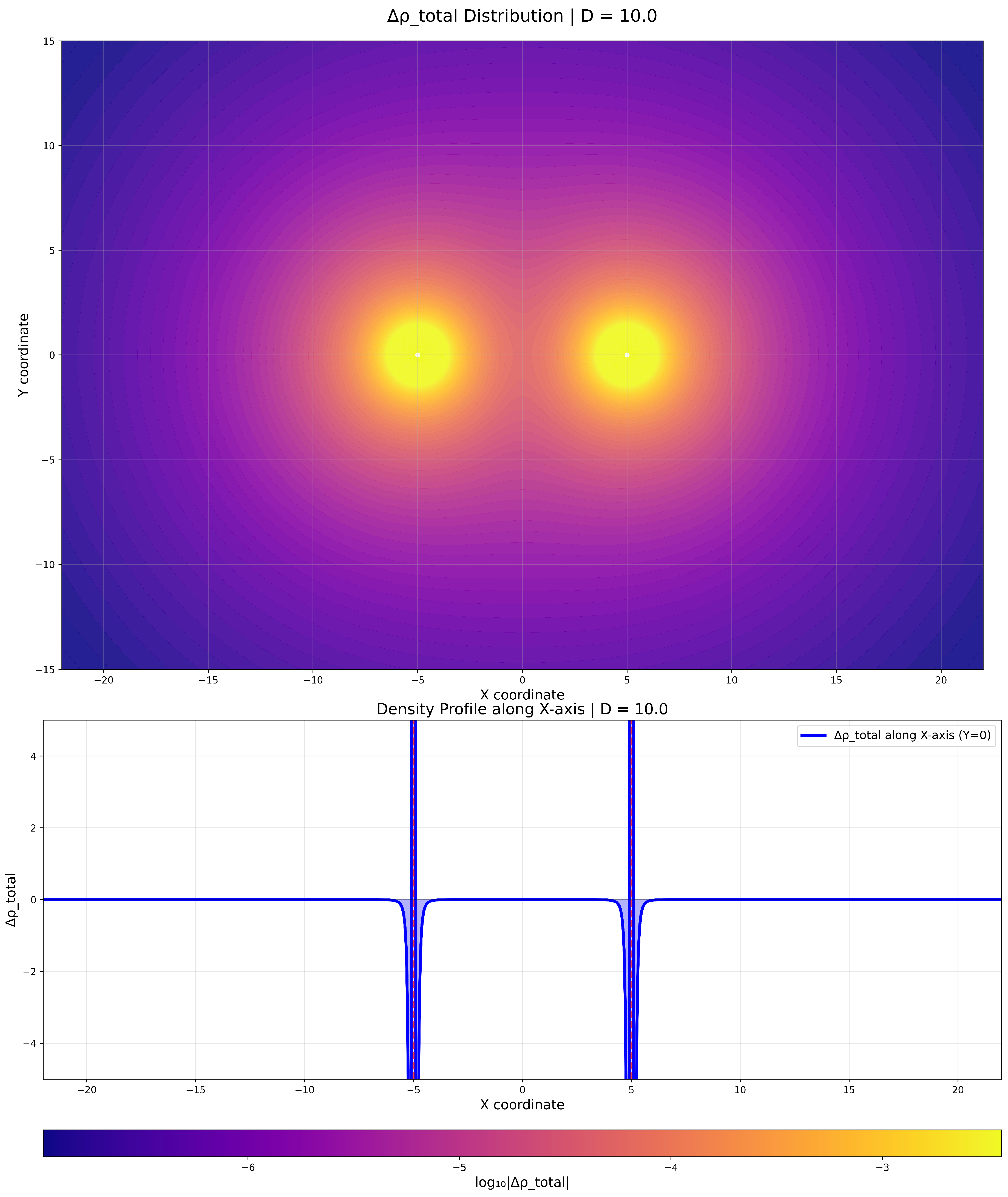
Figure 2. Visualization of the space density distribution for two spherical clusters

6. Verification of Space Density Quantity Conservation from Two Density Clusters. Integral of the Total Density Change in Three-Dimensional Volume

Let us verify how our postulate of space density quantity conservation holds in the case when it is determined by the change in the uniform density distribution from two density clusters. In the case of a single cluster, we confirmed that the total integral of the change in uniform density distribution, both inside the cluster and beyond its boundaries, equals zero. Let us check whether this postulate holds if the density perturbation is determined by the superposition of curvature coefficients from two clusters.

Consider the volume integral of the total change in space density:

$$I:={\int }_{{\mathbb{R}}^3}\Delta {\rho }_{\mathrm{total}}\left({\mathbf{r}}_1\right)d^3{r}_1.$$

Substituting the expansion

$$\Delta {\rho }_{\mathrm{total}}\left({\mathbf{r}}_1\right)=\Delta {\rho }_1\left({\mathbf{r}}_1\right)+\Delta {\rho }_2({\mathbf{r}}_1-\mathbf{D})+{\displaystyle \frac{\Delta {\rho }_1\left({\mathbf{r}}_1\right)\Delta {\rho }_2({\mathbf{r}}_1-\mathbf{D})}{{\rho }_0}},$$

we obtain the integral expansion:

$$I=I_1+I_2+{\displaystyle \frac{1}{{\rho }_0}}J,$$

where

$$I_1:={\int }_{{\mathbb{R}}^3}\Delta {\rho }_1\left({\mathbf{r}}_1\right)d^3{r}_1,I_2:={\int }_{{\mathbb{R}}^3}\Delta {\rho }_2({\mathbf{r}}_1-\mathbf{D})d^3{r}_1,$$

$$J:={\int }_{{\mathbb{R}}^3}\Delta {\rho }_1\left({\mathbf{r}}_1\right)\Delta {\rho }_2({\mathbf{r}}_1-\mathbf{D})d^3{r}_1.$$

Our goal is to show that $I_1=I_2=0$, whereas $J\ne 0$; this means that the total volume integral $I\ne 0$ and the postulate of "quantity" of density conservation is violated in the three-dimensional case.

—

6.1. Zeros of the First Two Integrals

For the first cluster

$$\Delta {\rho }_1\left({\mathbf{r}}_1\right)={\rho }_{1}H(R_1^{\prime }-r_1)-{\displaystyle \frac{{\rho }_1{R}_1^{\prime 4}}{3r_1^4}}H(r_1-R_1^{\prime }),$$

introduce spherical coordinates centered on the first cluster: $d^3{r}_1=4\pi r_1^{2}d{r}_1$. Then

$$I_1=4\pi \left[{\int }_0^{R_1^{\prime }}{\rho }_1{r}_1^{2}d{r}_1-{\int }_{R_1^{\prime }}^{\infty }{\displaystyle \frac{{\rho }_1{R}_1^{\prime 4}}{3r_1^4}}{r}_1^{2}d{r}_1\right].$$

Compute the integrals separately:

$${\int }_0^{R_1^{\prime }}{r}_1^{2}d{r}_1={\displaystyle \frac{R_1^{\prime 3}}{3}},{\int }_{R_1^{\prime }}^{\infty }{\displaystyle \frac{1}{r_1^2}}d{r}_1={\displaystyle \frac{1}{R_1^{\prime }}}.$$

Consequently,

$$I_1=4\pi {\rho }_1\left({\displaystyle \frac{R_1^{\prime 3}}{3}}-{\displaystyle \frac{R_1^{\prime 3}}{3}}\right)=0.$$

Similarly, for $I_2$ it suffices to make the variable change ${\mathbf{r}}^{\prime }={\mathbf{r}}_1-\mathbf{D}$, and we obtain

$$I_2={\int }_{{\mathbb{R}}^3}\Delta {\rho }_2\left({\mathbf{r}}^{\prime }\right)d^3{r}^{\prime }=0.$$

Thus,

$$I_1=I_2=0.$$

—

6.2. Nonlinear Term J

Decompose the product $\Delta {\rho }_1\left({\mathbf{r}}_1\right)\Delta {\rho }_2({\mathbf{r}}_1-\mathbf{D})$ into four terms corresponding to the internal (I) and external (O) regions of each cluster:

$$\begin{array}{cc}\hfill \Delta {\rho }_1& =\underset{{\mathrm{I}}_1}{\underbrace{{\rho }_{1}H(R_1^{\prime }-r_1)}}+\underset{{\mathrm{O}}_1}{\underbrace{-{\displaystyle \frac{{\rho }_1{R}_1^{\prime 4}}{3r_1^4}}H(r_1-R_1^{\prime })}},\hfill \\ \hfill \Delta {\rho }_2& =\underset{{\mathrm{I}}_2}{\underbrace{{\rho }_{2}H(R_2^{\prime }-|{\mathbf{r}}_1-\mathbf{D}\left|\right)}}+\underset{{\mathrm{O}}_2}{\underbrace{-{\displaystyle \frac{{\rho }_2{R}_2^{\prime 4}}{3|{\mathbf{r}}_1{-\mathbf{D}|}^4}}H\left(\right|{\mathbf{r}}_1-\mathbf{D}|-R_2^{\prime })}}.\hfill \end{array}$$

Then

$$J=J_{\mathrm{II}}+J_{\mathrm{IO}}+J_{\mathrm{OI}}+J_{\mathrm{OO}},$$

where, for example,

$$J_{\mathrm{OO}}={\int }_{\begin{array}{c}{r}_1>R_1^{\prime }\\ |{\mathbf{r}}_1-\mathbf{D}|>R_2^{\prime }\end{array}}{\displaystyle \frac{{\rho }_1{R}_1^{\prime 4}}{3r_1^4}}·{\displaystyle \frac{{\rho }_2{R}_2^{\prime 4}}{3|{\mathbf{r}}_1{-\mathbf{D}|}^4}}{d}^3{r}_1.$$

Since $\left({\mathrm{O}}_1\right)\left({\mathrm{O}}_2\right)>0$ on the intersection region of the external areas, and this region has non-zero volume, we obtain

$$J_{\mathrm{OO}}>0.$$

Consequently,

$$J={\int }_{{\mathbb{R}}^3}\Delta {\rho }_1\left({\mathbf{r}}_1\right)\Delta {\rho }_2({\mathbf{r}}_1-\mathbf{D})d^3{r}_1\ne 0({\rho }_1,{\rho }_2>0).$$

—

6.3. Conclusion: Violation of Integral Density Conservation in 3D

Since $I_1=I_2=0$, but $J\ne 0$, we have

$$I=I_1+I_2+{\displaystyle \frac{1}{{\rho }_0}}J={\displaystyle \frac{1}{{\rho }_0}}J\ne 0.$$

(6)

Therefore, the total volume integral of the density change, computed according to the correct multiplicative rule for combining curvature coefficients, is not zero in three-dimensional space. This means that within this model and in 3D, the integral ${\int }_{{\mathbb{R}}^3}\Delta {\rho }_{\mathrm{total}}{d}^{3}r$ is not equal to zero, i.e., the postulate of "quantity" of density conservation, which we defined when formulating the hypothesis about space density, is violated.

7. Transition to Five-Dimensional Space and Introduction of Interaction Operators

In three-dimensional space, the integral of the total density perturbation

$$I={\int }_{{\mathbb{R}}^3}\Delta {\rho }_{\mathrm{total}}\left(\mathbf{r}\right)d^{3}r$$

turned out to be non-zero, indicating the impossibility of strict density conservation when superimposing two curvatures within the framework of the three-dimensional model.

Moreover, the analytical computation of the cross integral

$$J={\int }_{{\mathbb{R}}^3}\Delta {\rho }_1\left(\mathbf{r}\right)\Delta {\rho }_2(\mathbf{r}-\mathbf{D})d^{3}r$$

in 3D space proves to be unsolvable in closed form, making it impossible to obtain an exact expression for the quantity of perturbation.

To overcome these limitations and correctly describe the interaction, a minimal five-dimensional space structure is introduced, allowing two three-dimensional subspaces to be treated as independent (orthogonal) but partially conjugated along one coordinate. This transition ensures a symmetric description of the interaction and restores the integral balance with the proper choice of metric.

7.1. Construction of the Five-Dimensional Space

Consider a space consisting of two three-dimensional subspaces, denoted as ${\mathbb{R}}_1^3$ and ${\mathbb{R}}_2^3$.

• The first subspace is defined by the coordinates:

  $$(r_{x_1},r_{y_1},r_{z_1},0,0),$$
• The second subspace — by the coordinates:

  $$(0,0,r_{z_2},r_{x_2},r_{y_2}).$$

All coordinates are orthogonal to each other, with the exception of the components $r_{z_1}$ and $r_{z_2}$, which are linked by a common direction — the Z-axis. They are connected through the displacement:

$$r_{z_2}=r_{z_1}-D,$$

where D is the distance between the centers of the two density clusters along the common axis.

Thus, the position vectors of the subspaces in the five-dimensional space take the form:

$$\begin{array}{cc}\hfill {\mathbf{r}}_1& =(r_{x_1},r_{y_1},r_{z_1},0,0),\hfill \\ \hfill {\mathbf{r}}_2& =(0,0,r_{z_2},r_{x_2},r_{y_2}).\hfill \end{array}$$

7.2. Scalar Product and Direct Interaction Operator

The scalar product of the position vectors in the five-dimensional space is:

$${\mathbf{r}}_1·{\mathbf{r}}_2=r_{z_1}{r}_{z_2}.$$

Based on this, the direct interaction operator between the subspaces is introduced:

$$T_{12}={\displaystyle \frac{{\mathbf{r}}_1·{\mathbf{r}}_2}{|{\mathbf{r}}_1\left|\right|{\mathbf{r}}_2|}}={\displaystyle \frac{r_{z_1}{r}_{z_2}}{|{\mathbf{r}}_1\left|\right|{\mathbf{r}}_2|}}.$$

(7)

The operator $T_{12}$ determines the degree of projection of subspace ${\mathbb{R}}_1^3$ onto subspace ${\mathbb{R}}_2^3$ along the common Z-axis. It describes directed interaction — the influence of the first coordinate system on the second in the five-dimensional metric.

The transition to a five-dimensional description allows the interaction to be separated by subspaces while maintaining the overall geometric connection. Thanks to this, it becomes possible to formalize the nonlinear term in the Lagrangian not as "multiplication of functions in one volume", but as a scalar convolution in different subspaces.

7.3. Inverse Interaction Operator

Similarly, the inverse interaction operator is introduced, accounting for the projection of the second subspace onto the first:

$$T_{21}={\displaystyle \frac{(r_{z_2}+D)(r_{z_1}-D)}{|{\mathbf{r}}_2+D\left|\right|{\mathbf{r}}_1-D|}}.$$

Here, the mutual relations are used:

$$\begin{array}{cc}\hfill r_{z_1}& =r_{z_2}+D,\hfill \\ \hfill r_{z_2}& =r_{z_1}-D.\hfill \end{array}$$

Thus, $T_{21}$ represents the operator action of $T_{12}$ in the reverse direction: it models the inverse projection ${\mathbb{R}}_2^3\to {\mathbb{R}}_1^3$.

7.4. Asymmetry of Operators Under Integration

Although the numerical values of $T_{12}$ and $T_{21}$ may coincide, their action under integration is different, since:

• the integral over the first subspace is performed over the coordinates $(r_{x_1},r_{y_1},r_{z_1})$,
• the integral over the second — over $(r_{x_2},r_{y_2},r_{z_2})$, and the projections onto the Z-axis have different orientations.

This geometric asymmetry of the operators ensures the appearance of a cross term in the Lagrangian, which accounts not merely for the product of perturbations, but for their spatial coordination in different subspaces. Thus, the transition to 5D allows for a correct description of the interaction between density clusters as a result of mutual projections of curvatures of the uniform density distribution of space.

The five-dimensional construction eliminates the problem of conserving the quantity of space density from the three-dimensional model, because now the densities belong to different subspaces, and their interaction is described not by a sum or product, but by the projection operator $T_{12}-T_{21}$, which correctly coordinates the transfer of interaction between the three-dimensional subspaces of the 5D space.

8. Satisfaction of the Space Density Conservation Law in 5D with the Direct Interaction Operator $T_{12}$

In Section VI of our investigation, we found that the integral over the entire space of the space density distribution determined by two clusters (via curvature coefficients) is not equal to zero, which violates our postulate on the conservation of the quantity of space density. Let us check how this postulate holds in 5D space.

Let us define the quantity of interaction between two density clusters as the integral of the total density distribution over the entire 5D space, but taking into account the interaction operator that determines the effect of the perturbation of one subspace on the other:

$$W_{12}:={\int }_{{\mathbb{R}}^3}{\int }_{{\mathbb{R}}^3}\Delta {\rho }_{\mathrm{total}}({\mathbf{r}}_1,{\mathbf{r}}_2)T_{12}({\mathbf{r}}_1,{\mathbf{r}}_2)d^3{r}_1{d}^3{r}_2,$$

(8)

where in the 5D formulation, the decomposition

$$\Delta {\rho }_{\mathrm{total}}({\mathbf{r}}_1,{\mathbf{r}}_2)=\Delta {\rho }_1\left({\mathbf{r}}_1\right)+\Delta {\rho }_2\left({\mathbf{r}}_2\right)+{\displaystyle \frac{1}{{\rho }_0}}\Delta {\rho }_1\left({\mathbf{r}}_1\right)\Delta {\rho }_2\left({\mathbf{r}}_2\right)$$

is used, and the direct interaction operator is given by

$$T_{12}({\mathbf{r}}_1,{\mathbf{r}}_2)={\displaystyle \frac{{\mathbf{r}}_1·{\mathbf{r}}_2}{|{\mathbf{r}}_1\left|\right|{\mathbf{r}}_2|}}={\displaystyle \frac{r_{z_1}{r}_{z_2}}{|{\mathbf{r}}_1\left|\right|{\mathbf{r}}_2|}}.$$

Substituting the decomposition of $\Delta {\rho }_{\mathrm{total}}$ into $W_{12}$, we expand the integral into three terms:

$$W_{12}=W^{\left(1\right)}+W^{\left(2\right)}+W^{(\times )},$$

where

$$\begin{array}{cc}\hfill W^{\left(1\right)}& ={\int }_{{\mathbb{R}}^3}{\int }_{{\mathbb{R}}^3}\Delta {\rho }_1\left({\mathbf{r}}_1\right)T_{12}({\mathbf{r}}_1,{\mathbf{r}}_2)d^3{r}_1{d}^3{r}_2,\hfill \\ \hfill W^{\left(2\right)}& ={\int }_{{\mathbb{R}}^3}{\int }_{{\mathbb{R}}^3}\Delta {\rho }_2\left({\mathbf{r}}_2\right)T_{12}({\mathbf{r}}_1,{\mathbf{r}}_2)d^3{r}_1{d}^3{r}_2,\hfill \\ \hfill W^{(\times )}& ={\displaystyle \frac{1}{{\rho }_0}}{\int }_{{\mathbb{R}}^3}{\int }_{{\mathbb{R}}^3}\Delta {\rho }_1\left({\mathbf{r}}_1\right)\Delta {\rho }_2\left({\mathbf{r}}_2\right)T_{12}({\mathbf{r}}_1,{\mathbf{r}}_2)d^3{r}_1{d}^3{r}_2.\hfill \end{array}$$

For further transformations, it is convenient to separate the angular and radial variables in each subspace. Let us denote the standard spherical coordinates in the first subspace by $(r_1,{\theta }_1,{\phi }_1)$, and in the second by $(r_2,{\theta }_2,{\phi }_2)$. Then:

$${\displaystyle \frac{r_{z_1}}{|{\mathbf{r}}_1|}}=\cos {\theta }_1,{\displaystyle \frac{r_{z_2}}{|{\mathbf{r}}_2|}}=\cos {\theta }_2,$$

and the volume measure takes the form:

$$d^3{r}_1=r_1^{2}d{r}_{1}d{\Omega }_1,d^3{r}_2=r_2^{2}d{r}_{2}d{\Omega }_2,$$

where $d{\Omega }_i=\sin {\theta }_{i}d{\theta }_{i}d{\phi }_i$ is the elementary solid angle on the sphere $S^2$.

Substituting $T_{12}=\cos {\theta }_1\cos {\theta }_2$ into the expressions for $W^{\left(1\right)},W^{\left(2\right)},W^{(\times )}$, we obtain factorization over angles and radii.

For $W^{\left(1\right)}$:

$$\begin{array}{cc}\hfill W^{\left(1\right)}& ={\int }_0^{\infty }{\int }_0^{\infty }\left[\Delta {\rho }_1\left(r_1\right)r_1^{2}d{r}_1\right]\left[r_2^{2}d{r}_2\right]\hfill \\ \hfill & \times \left[{\int }_{S^2}\cos {\theta }_{1}d{\Omega }_1\right]\left[{\int }_{S^2}\cos {\theta }_{2}d{\Omega }_2\right].\hfill \end{array}$$

Similarly for $W^{\left(2\right)}$:

$$\begin{array}{cc}\hfill W^{\left(2\right)}& ={\int }_0^{\infty }{\int }_0^{\infty }\left[r_1^{2}d{r}_1\right]\left[\Delta {\rho }_2\left(r_2\right)r_2^{2}d{r}_2\right]\hfill \\ \hfill & \times \left[{\int }_{S^2}\cos {\theta }_{1}d{\Omega }_1\right]\left[{\int }_{S^2}\cos {\theta }_{2}d{\Omega }_2\right].\hfill \end{array}$$

For the cross term $W^{(\times )}$, we have complete factorization:

$$\begin{array}{cc}\hfill W^{(\times )}& ={\displaystyle \frac{1}{{\rho }_0}}\left({\int }_0^{\infty }\Delta {\rho }_1\left(r_1\right)r_1^{2}d{r}_1{\int }_{S^2}\cos {\theta }_{1}d{\Omega }_1\right)\hfill \\ \hfill & \times \left({\int }_0^{\infty }\Delta {\rho }_2\left(r_2\right)r_2^{2}d{r}_2{\int }_{S^2}\cos {\theta }_{2}d{\Omega }_2\right).\hfill \end{array}$$

Key observation: on the sphere, the following holds

$$\begin{array}{cc}\hfill {\int }_{S^2}\cos \theta d\Omega & ={\int }_0^{2\pi }d\phi {\int }_0^{\pi }\cos \theta \sin \theta d\theta \hfill \\ \hfill & =2\pi {\left[\frac{1}{2}{\sin }^2\theta \right]}_0^{\pi }=0.\hfill \end{array}$$

Consequently, each angular integral term equals zero:

$${\int }_{S^2}\cos {\theta }_{1}d{\Omega }_1=0,{\int }_{S^2}\cos {\theta }_{2}d{\Omega }_2=0.$$

From this it directly follows:

$$W^{\left(1\right)}=0,W^{\left(2\right)}=0,W^{(\times )}=0,$$

and hence:

$$W_{12}=0.$$

Thus, when using the direct interaction operator $T_{12}$ in the five-dimensional formalism, the integral of the total perturbation, taken with the weight $T_{12}$, vanishes. This means the restoration of the volumetric law of "conservation of the quantity of density" in the proposed 5D model: the projection mechanisms between subspaces yield a zero total contribution after integration over all angles of both subspaces.

9. Definition of the Integral $W_{21}$ with the Inverse Interaction Operator in 5D

Let us define the integral:

$$W_{21}:={\int }_{{\mathbb{R}}^3}{\int }_{{\mathbb{R}}^3}\Delta {\rho }_{\mathrm{total}}({\mathbf{r}}_1,{\mathbf{r}}_2)T_{21}({\mathbf{r}}_1,{\mathbf{r}}_2)d^3{r}_1{d}^3{r}_2,$$

where the inverse interaction operator is given by:

$$T_{21}({\mathbf{r}}_1,{\mathbf{r}}_2)={\displaystyle \frac{(r_{z_2}+D)(r_{z_1}-D)}{|{\mathbf{r}}_2+D\left|\right|{\mathbf{r}}_1-D|}},$$

and the deviation of the density distribution from uniform is determined by the formula:

$$\Delta {\rho }_{\mathrm{total}}({\mathbf{r}}_1,{\mathbf{r}}_2)=\Delta {\rho }_1\left({\mathbf{r}}_1\right)+\Delta {\rho }_2\left({\mathbf{r}}_2\right)+{\displaystyle \frac{1}{{\rho }_0}}\Delta {\rho }_1\left({\mathbf{r}}_1\right)\Delta {\rho }_2\left({\mathbf{r}}_2\right).$$

Substituting both expressions into the integral $W_{21}$, we obtain an expansion into three terms:

$$\begin{array}{cc}\hfill W_{21}& =\underset{W_{21}^{\left(1\right)}}{\underbrace{{\int }_{{\mathbb{R}}^3}{\int }_{{\mathbb{R}}^3}\Delta {\rho }_1\left({\mathbf{r}}_1\right)T_{21}({\mathbf{r}}_1,{\mathbf{r}}_2)d^3{r}_1{d}^3{r}_2}}\hfill \\ \hfill & +\underset{W_{21}^{\left(2\right)}}{\underbrace{{\int }_{{\mathbb{R}}^3}{\int }_{{\mathbb{R}}^3}\Delta {\rho }_2\left({\mathbf{r}}_2\right)T_{21}({\mathbf{r}}_1,{\mathbf{r}}_2)d^3{r}_1{d}^3{r}_2}}\hfill \\ \hfill & +\underset{W_{21}^{(\times )}}{\underbrace{{\displaystyle \frac{1}{{\rho }_0}}{\int }_{{\mathbb{R}}^3}{\int }_{{\mathbb{R}}^3}\Delta {\rho }_1\left({\mathbf{r}}_1\right)\Delta {\rho }_2\left({\mathbf{r}}_2\right)T_{21}({\mathbf{r}}_1,{\mathbf{r}}_2)d^3{r}_1{d}^3{r}_2}}.\hfill \end{array}$$

Let us substitute the formulas for the space density distribution of each cluster into the expression for the perturbation quantity

Local density perturbations in each subspace have the form:

$$\begin{array}{cc}\hfill \Delta {\rho }_1\left({\mathbf{r}}_1\right)& ={\rho }_{1}H(R_1^{\prime }-r_1)-{\displaystyle \frac{{\rho }_1{R}_1^{\prime 4}}{3r_1^4}}H(r_1-R_1^{\prime }),\hfill \\ \hfill \Delta {\rho }_2\left({\mathbf{r}}_2\right)& ={\rho }_{2}H(R_2^{\prime }-r_2)-{\displaystyle \frac{{\rho }_2{R}_2^{\prime 4}}{3r_2^4}}H(r_2-R_2^{\prime }),\hfill \end{array}$$

where $H\left(x\right)$ is the Heaviside function, $R_i^{\prime }$ are the effective radii of the clusters, and ${\rho }_i$ are their internal densities. Then each term of the integral can be written explicitly:

1. First term:

$$\begin{array}{cc}\hfill W_{21}^{\left(1\right)}& ={\int }_{{\mathbb{R}}^3}{\int }_{{\mathbb{R}}^3}\left[{\rho }_{1}H(R_1^{\prime }-r_1)-{\displaystyle \frac{{\rho }_1{R}_1^{\prime 4}}{3r_1^4}}H(r_1-R_1^{\prime })\right]\hfill \\ \hfill & \times {\displaystyle \frac{(r_{z_2}+D)(r_{z_1}-D)}{|{\mathbf{r}}_2+D\left|\right|{\mathbf{r}}_1-D|}}{d}^3{r}_1{d}^3{r}_2.\hfill \end{array}$$

2. Second term:

$$\begin{array}{cc}\hfill W_{21}^{\left(2\right)}& ={\int }_{{\mathbb{R}}^3}{\int }_{{\mathbb{R}}^3}\left[{\rho }_{2}H(R_2^{\prime }-r_2)-{\displaystyle \frac{{\rho }_2{R}_2^{\prime 4}}{3r_2^4}}H(r_2-R_2^{\prime })\right]\hfill \\ \hfill & \times {\displaystyle \frac{(r_{z_2}+D)(r_{z_1}-D)}{|{\mathbf{r}}_2+D\left|\right|{\mathbf{r}}_1-D|}}{d}^3{r}_1{d}^3{r}_2.\hfill \end{array}$$

3. Cross term:

$$\begin{array}{cc}\hfill W_{21}^{(\times )}& ={\displaystyle \frac{1}{{\rho }_0}}{\int }_{{\mathbb{R}}^3}{\int }_{{\mathbb{R}}^3}\left[{\rho }_{1}H(R_1^{\prime }-r_1)-{\displaystyle \frac{{\rho }_1{R}_1^{\prime 4}}{3r_1^4}}H(r_1-R_1^{\prime })\right]\hfill \\ \hfill & \times \left[{\rho }_{2}H(R_2^{\prime }-r_2)-{\displaystyle \frac{{\rho }_2{R}_2^{\prime 4}}{3r_2^4}}H(r_2-R_2^{\prime })\right]\hfill \\ \hfill & \times {\displaystyle \frac{(r_{z_2}+D)(r_{z_1}-D)}{|{\mathbf{r}}_2+D\left|\right|{\mathbf{r}}_1-D|}}{d}^3{r}_1{d}^3{r}_2.\hfill \end{array}$$

This is the final expression for the integral $W_{21}$ as an integral over ${\mathbb{R}}^3\times {\mathbb{R}}^3$ taking into account the inverse interaction operator and the explicit functions $\Delta {\rho }_1$ and $\Delta {\rho }_2$.

For convenience, let us represent the cross term of the integral $W_{21}$ as a product of integrals over subspaces

Let us denote the expressions for local density perturbations as:

$$\begin{array}{cc}\hfill I_{{\mathbb{R}}_1^3}& ={\int }_{{\mathbb{R}}^3}\left[{\rho }_{1}H(R_1^{\prime }-r_1)-{\displaystyle \frac{{\rho }_1{R}_1^{\prime 4}}{3r_1^4}}H(r_1-R_1^{\prime })\right]{\displaystyle \frac{r_{z_1}-D}{|{\mathbf{r}}_1-D|}}{d}^3{r}_1,\hfill \\ \hfill I_{{\mathbb{R}}_2^3}& ={\int }_{{\mathbb{R}}^3}\left[{\rho }_{2}H(R_2^{\prime }-r_2)-{\displaystyle \frac{{\rho }_2{R}_2^{\prime 4}}{3r_2^4}}H(r_2-R_2^{\prime })\right]{\displaystyle \frac{r_{z_2}+D}{|{\mathbf{r}}_2+D|}}{d}^3{r}_2.\hfill \end{array}$$

Then the cross term $W_{21}^{(\times )}$ can be written in factorized form:

$$W_{21}^{(\times )}={\displaystyle \frac{1}{{\rho }_0}}{I}_{{\mathbb{R}}_1^3}{I}_{{\mathbb{R}}_2^3}.$$

Thus, the cross term of the integral $W_{21}^{(\times )}$ reduces to the product of two three-dimensional integrals, each describing the contribution of its own subspace. This factorization emphasizes the fundamental feature of the five-dimensional formalism: the interaction between two density clusters is represented as the result of the joint action of integrals over two three-dimensional subspaces, which restores the symmetry of the system and ensures correct conservation of the total density quantity after integration.

9.1. Computation of the Integral $I_{{\mathbb{R}}_1^3}$

Let us switch to spherical coordinates $(r_1,{\theta }_1,{\phi }_1)$ centered on the first cluster:

$$r_{x_1}=r_1\sin {\theta }_1\cos {\phi }_1,r_{y_1}=r_1\sin {\theta }_1\sin {\phi }_1,r_{z_1}=r_1\cos {\theta }_1.$$

The volume element then takes the form:

$$d^3{r}_1=r_1^2\sin {\theta }_{1}d{r}_{1}d{\theta }_{1}d{\phi }_1,$$

and the fraction in the integrand becomes:

$${\displaystyle \frac{r_{z_1}-D}{|{\mathbf{r}}_1-D|}}={\displaystyle \frac{r_1\cos {\theta }_1-D}{\sqrt{r_1^2-2D{r}_1\cos {\theta }_1+D^2}}}.$$

Substituting all this into the integral, we get:

$$\begin{array}{cc}\hfill I_{{\mathbb{R}}_1^3}& ={\int }_0^{\infty }{r}_1^{2}d{r}_1{\int }_0^{\pi }\sin {\theta }_{1}d{\theta }_1{\int }_0^{2\pi }d{\phi }_1\hfill \\ \hfill & \times \left[{\rho }_{1}H(R_1^{\prime }-r_1)-{\displaystyle \frac{{\rho }_1{R}_1^{\prime 4}}{3r_1^4}}H(r_1-R_1^{\prime })\right]{\displaystyle \frac{r_1\cos {\theta }_1-D}{\sqrt{r_1^2-2D{r}_1\cos {\theta }_1+D^2}}}.\hfill \end{array}$$

The integral over the azimuthal angle is trivial:

$${\int }_0^{2\pi }d{\phi }_1=2\pi .$$

Consequently,

$$\begin{array}{cc}\hfill I_{{\mathbb{R}}_1^3}& =2\pi {\int }_0^{\infty }{r}_1^{2}d{r}_1{\int }_0^{\pi }\sin {\theta }_1\hfill \\ \hfill & \times \left[{\rho }_{1}H(R_1^{\prime }-r_1)-{\displaystyle \frac{{\rho }_1{R}_1^{\prime 4}}{3r_1^4}}H(r_1-R_1^{\prime })\right]{\displaystyle \frac{r_1\cos {\theta }_1-D}{\sqrt{r_1^2-2D{r}_1\cos {\theta }_1+D^2}}}d{\theta }_1.\hfill \end{array}$$

9.2. Separation into Internal and External Regions

1. Internal region $(r_1<R_1^{\prime })$:

$$\begin{array}{cc}\hfill I_{{\mathbb{R}}_1^3}^{\left(\mathrm{in}\right)}& =2\pi {\rho }_1{\int }_0^{R_1^{\prime }}{r}_1^{2}d{r}_1{\int }_0^{\pi }\sin {\theta }_1\hfill \\ \hfill & \times {\displaystyle \frac{r_1\cos {\theta }_1-D}{\sqrt{r_1^2-2D{r}_1\cos {\theta }_1+D^2}}}d{\theta }_1.\hfill \end{array}$$

2. External region $(r_1>R_1^{\prime })$:

$$\begin{array}{cc}\hfill I_{{\mathbb{R}}_1^3}^{\left(\mathrm{out}\right)}& =-{\displaystyle \frac{2\pi {\rho }_1{R}_1^{\prime 4}}{3}}{\int }_{R_1^{\prime }}^{\infty }{\displaystyle \frac{d{r}_1}{r_1^2}}{\int }_0^{\pi }\sin {\theta }_1\hfill \\ \hfill & \times {\displaystyle \frac{r_1\cos {\theta }_1-D}{\sqrt{r_1^2-2D{r}_1\cos {\theta }_1+D^2}}}d{\theta }_1.\hfill \end{array}$$

Thus,

$$I_{{\mathbb{R}}_1^3}=I_{{\mathbb{R}}_1^3}^{\left(\mathrm{in}\right)}+I_{{\mathbb{R}}_1^3}^{\left(\mathrm{out}\right)}.$$

Integration over the angle ${\theta }_1$

Let $u=\cos {\theta }_1$, then $\sin {\theta }_{1}d{\theta }_1=-du$, $u\in [-1,1]$. The integral over ${\theta }_1$ is rewritten as:

$$J_1\left(r_1\right)={\int }_{-1}^1{\displaystyle \frac{r_{1}u-D}{\sqrt{r_1^2-2D{r}_{1}u+D^2}}}du.$$

Make the substitution $t=r_1^2+D^2-2r_{1}Du\Rightarrow dt=-2r_{1}Ddu$, with limits $u=-1\Rightarrow t={(r_1+D)}^2$, $u=1\Rightarrow t={(r_1-D)}^2$. Then:

$$J_1\left(r_1\right)={\displaystyle \frac{1}{4r_{1}D}}{\int }_{{(r_1-D)}^2}^{{(r_1+D)}^2}{\displaystyle \frac{r_1^2-D^2-t}{\sqrt{t}}}dt.$$

The antiderivative gives:

$$\int {\displaystyle \frac{r_1^2-D^2-t}{\sqrt{t}}}dt=2(r_1^2-D^2)\sqrt{t}-{\displaystyle \frac{2}{3}}{t}^{3/2}.$$

Substituting the limits ${(r_1-D)}^2$ and ${(r_1+D)}^2$:

$$J_1\left(r_1\right)={\displaystyle \frac{1}{2r_1{D}^2}}\left[(r_1^2-D^2)((r_1+D)-|r_1-D\left|\right)-{\displaystyle \frac{1}{3}}({(r_1+D)}^3-|r_1-D{|}^3)\right].$$

Split by regions:

$$\left\{\begin{array}{cc}{r}_1<D:\hfill & J_1\left(r_1\right)=-2\left(1-{\displaystyle \frac{r_1^2}{3D^2}}\right),\hfill \\ r_1>D:\hfill & J_1\left(r_1\right)=-{\displaystyle \frac{4}{3}}{\displaystyle \frac{D}{r_1}}.\hfill \end{array}\right.$$

Volume part

Multiply by $2\pi r_1^2$ for the volume measure:

$$A_1\left(r_1\right)=2\pi r_1^2{J}_1\left(r_1\right)=\left\{\begin{array}{cc}-4\pi r_1^2\left(1-{\displaystyle \frac{r_1^2}{3D^2}}\right),\hfill & r_1<D,\hfill \\ -{\displaystyle \frac{8\pi }{3}}D{r}_1,\hfill & r_1>D.\hfill \end{array}\right.$$

Splitting the integral using the Heaviside function

Taking into account the internal and external parts of $\Delta {\rho }_1\left({\mathbf{r}}_1\right)$, we obtain a one-dimensional integral:

$$I_{{\mathbb{R}}_1^3}={\int }_0^{R_1^{\prime }}{A}_1\left(r_1\right)d{r}_1-{\displaystyle \frac{R_1^{\prime 4}}{3}}{\int }_{R_1^{\prime }}^{\infty }{\displaystyle \frac{A_1\left(r_1\right)}{r_1^4}}d{r}_1.$$

1. Internal integral:

$$\begin{array}{cc}\hfill {\int }_0^{R_1}{A}_1\left(r_1\right)d{r}_1& ={\int }_0^{R_1}-4\pi r_1^2\left(1-{\displaystyle \frac{r_1^2}{3D^2}}\right)d{r}_1\hfill \\ \hfill & =-4\pi \left({\displaystyle \frac{R_1^3}{3}}-{\displaystyle \frac{R_1^5}{15D^2}}\right).\hfill \end{array}$$

2. External integral:

$$\begin{array}{cc}\hfill {\int }_{R_1}^{\infty }{\displaystyle \frac{A_1\left(r_1\right)}{r_1^4}}d{r}_1& ={\int }_{R_1}^D-4\pi \left({\displaystyle \frac{1}{r_1^2}}-{\displaystyle \frac{1}{3D^2}}\right)d{r}_1+{\int }_D^{\infty }-{\displaystyle \frac{8\pi }{3}}{\displaystyle \frac{D}{r_1^3}}d{r}_1\hfill \\ \hfill & =-4\pi \left({\displaystyle \frac{1}{R_1}}-{\displaystyle \frac{1}{3D}}+{\displaystyle \frac{R_1}{3D^2}}\right).\hfill \end{array}$$

3. Combining $I_{{\mathbb{R}}_1^3}$:

$$\begin{array}{cc}\hfill I_{{\mathbb{R}}_1^3}& ={\rho }_1\left[-4\pi \left({\displaystyle \frac{R_1^3}{3}}-{\displaystyle \frac{R_1^5}{15D^2}}\right)-{\displaystyle \frac{R_1^4}{3}}\left(-4\pi \left({\displaystyle \frac{1}{R_1}}-{\displaystyle \frac{1}{3D}}+{\displaystyle \frac{R_1}{3D^2}}\right)\right)\right]\hfill \\ \hfill & ={\rho }_1{\displaystyle \frac{4\pi R_1^4}{45D^2}}(8R_1-15D),R_1<D.\hfill \end{array}$$

1. Internal integral:

$$\begin{array}{cc}\hfill {\int }_0^{R_1}{A}_1\left(r_1\right)d{r}_1& ={\int }_0^D-4\pi r_1^2\left(1-{\displaystyle \frac{r_1^2}{3D^2}}\right)d{r}_1+{\int }_D^{R_1}-{\displaystyle \frac{8\pi }{3}}D{r}_{1}d{r}_1\hfill \\ \hfill & =-{\displaystyle \frac{8\pi D}{9}}{R}_1^2+{\displaystyle \frac{4\pi }{15}}{D}^3.\hfill \end{array}$$

2. External integral:

$${\int }_{R_1}^{\infty }{\displaystyle \frac{A_1\left(r_1\right)}{r_1^4}}d{r}_1={\int }_{R_1}^{\infty }-{\displaystyle \frac{8\pi }{3}}{\displaystyle \frac{D}{r_1^3}}d{r}_1=-{\displaystyle \frac{4\pi D}{3R_1^2}}.$$

3. Combining $I_{{\mathbb{R}}_1^3}$:

$$I_{{\mathbb{R}}_1^3}={\rho }_1{\displaystyle \frac{4\pi D}{45}}(3D^2-10R_1^2),R_1\ge D.$$

9.3. Calculation of the integral $I_{{\mathbb{R}}_2^3}$ from symmetry considerations the relation $J_2=-J_1$ should hold, let us verify this

Consider the integral over the second subspace:

$$I_{{\mathbb{R}}_2^3}={\int }_{{\mathbb{R}}^3}\Delta {\rho }_2\left({\mathbf{r}}_2\right){\displaystyle \frac{r_{z_2}+D}{|{\mathbf{r}}_2+D|}}{d}^3{r}_2,$$

where

$$\Delta {\rho }_2\left({\mathbf{r}}_2\right)={\rho }_{2}H(R_2^{\prime }-r_2)-{\displaystyle \frac{{\rho }_2{R}_2^{\prime 4}}{3r_2^4}}H(r_2-R_2^{\prime }).$$

9.3.0.12. Case 1: $R_2<D$

$${\int }_0^{R_2}{A}_2\left(r_2\right)d{r}_2={\int }_0^{R_2}-A_1\left(r_2\right)d{r}_2=-{\int }_0^{R_2}{A}_1\left(r_2\right)d{r}_2,$$

$${\int }_{R_2}^{\infty }{\displaystyle \frac{A_2\left(r_2\right)}{r_2^4}}d{r}_2=-{\int }_{R_2}^{\infty }{\displaystyle \frac{A_1\left(r_2\right)}{r_2^4}}d{r}_2.$$

Therefore,

$$I_{{\mathbb{R}}_2^3}=-I_{{\mathbb{R}}_1^3}={\rho }_2{\displaystyle \frac{4\pi R_2^4}{45D^2}}(15D-8R_2),R_2<D.$$

9.3.0.13. Case 2: $R_2\ge D$

$${\int }_0^{R_2}{A}_2\left(r_2\right)d{r}_2=-{\int }_0^{R_2}{A}_1\left(r_2\right)d{r}_2,{\int }_{R_2}^{\infty }{\displaystyle \frac{A_2\left(r_2\right)}{r_2^4}}d{r}_2=-{\int }_{R_2}^{\infty }{\displaystyle \frac{A_1\left(r_2\right)}{r_2^4}}d{r}_2,$$

then

$$I_{{\mathbb{R}}_2^3}=-I_{{\mathbb{R}}_1^3}={\rho }_2{\displaystyle \frac{4\pi D}{45}}(10R_2^2-3D^2),R_2\ge D.$$

From the obtained integral computations, we see that indeed $J_2=-J_1$.

9.4. Based on the Computations, Find the Final Expression for the Cross Term $W_{21}^{\times }$ for the Case $D>R_1,R_2$

Expanding the brackets for $I_{R_1^3}$ when $D>R_1$

$$I_{R_1^3}={\rho }_1{\displaystyle \frac{4\pi R_1^4}{45D^2}}(8R_1-15D)={\rho }_1{\displaystyle \frac{32\pi R_1^5}{45D^2}}-{\rho }_1{\displaystyle \frac{4\pi R_1^4}{3D}}.$$

Similarly for $I_{R_2^3}$ when $D>R_2$

$$I_{R_2^3}={\rho }_2{\displaystyle \frac{32\pi R_2^5}{45D^2}}-{\rho }_2{\displaystyle \frac{4\pi R_2^4}{3D}}.$$

Expression in terms of charges $Q_1,Q_2$

$$Q_1={\rho }_1{\displaystyle \frac{4\pi R_1^3}{3}},Q_2={\rho }_2{\displaystyle \frac{4\pi R_2^3}{3}},$$

$$I_{R_1^3}={\displaystyle \frac{8}{15}}{\displaystyle \frac{Q_1{R}_1^2}{D^2}}-{\displaystyle \frac{Q_1{R}_1}{D}},I_{R_2^3}={\displaystyle \frac{8}{15}}{\displaystyle \frac{Q_2{R}_2^2}{D^2}}-{\displaystyle \frac{Q_2{R}_2}{D}}.$$

Cross term $W_{21}^{\times }$

$$W_{21}^{\times }={\displaystyle \frac{1}{{\rho }_0}}{I}_{R_1^3}{I}_{R_2^3}={\displaystyle \frac{1}{{\rho }_0}}\left({\displaystyle \frac{8}{15}}{\displaystyle \frac{Q_1{R}_1^2}{D^2}}-{\displaystyle \frac{Q_1{R}_1}{D}}\right)\left({\displaystyle \frac{8}{15}}{\displaystyle \frac{Q_2{R}_2^2}{D^2}}-{\displaystyle \frac{Q_2{R}_2}{D}}\right).$$

Compact expression

$$W_{21}^{\times }={\displaystyle \frac{1}{{\rho }_0}}\left({\displaystyle \frac{8Q_1{R}_1^2}{15D^2}}-{\displaystyle \frac{Q_1{R}_1}{D}}\right)\left({\displaystyle \frac{8Q_2{R}_2^2}{15D^2}}-{\displaystyle \frac{Q_2{R}_2}{D}}\right),D>R_1,R_2.$$

After multiplying the brackets, we obtain the expression:

$$\begin{array}{cc}\hfill W_{21}^{\times }& ={\displaystyle \frac{1}{{\rho }_0}}[\left({\displaystyle \frac{8Q_1{R}_1^2}{15D^2}}\right)\left({\displaystyle \frac{8Q_2{R}_2^2}{15D^2}}\right)-\left({\displaystyle \frac{8Q_1{R}_1^2}{15D^2}}\right)\left({\displaystyle \frac{Q_2{R}_2}{D}}\right)\hfill \\ & -\left({\displaystyle \frac{Q_1{R}_1}{D}}\right)\left({\displaystyle \frac{8Q_2{R}_2^2}{15D^2}}\right)+\left({\displaystyle \frac{Q_1{R}_1}{D}}\right)\left({\displaystyle \frac{Q_2{R}_2}{D}}\right)].\hfill \end{array}$$

10. Computation of the Perturbation Quantities $W_{21}^{\left(1\right)}$, $W_{21}^{\left(2\right)}$ Separation of the Interaction Operator over Three-Dimensional Subspaces

When integrating a three-dimensional function belonging to only one 3D subspace over the entire 5D space, taking into account the inverse interaction operator $T_{21}$ between two three-dimensional subspaces, we encounter a divergence problem. This is because it is incorrect to integrate any part of the interaction operator over the entire subspace without a function describing the distribution of density change relative to ${\rho }_0$ over this subspace.

To eliminate this problem, it is proposed to use "half" convolution operators $\left(T_2\right)$ and $\left(T_1\right)$, which allows to correctly separate the interaction and isolate the amount of perturbation created by each charge separately on the opposite subspace.

10.1. Method of Operator Separation

For $W_{21}^{\left(1\right)}$

• We take the integral only over ${\mathbf{r}}_1$, over the three-dimensional space of charge 1.
• We apply the operator $T_2$ — half of the inverse interaction operator $T_{21}$, leaving only the component ${\mathbf{r}}_2/\left|{\mathbf{r}}_2\right|$.
• As a result, we obtain the potential created by charge 1, denoted by $W_2^{\left(1\right)}$.

For $W_{21}^{\left(2\right)}$

• We take the integral only over ${\mathbf{r}}_2$, over the three-dimensional space of charge 2.
• We apply the operator $T_1$ — half of the inverse interaction operator $T_{21}$, leaving only the component ${\mathbf{r}}_1/\left|{\mathbf{r}}_1\right|$.
• As a result, we obtain the potential created by charge 2, denoted by $W_1^{\left(2\right)}$.

Thus, instead of the infinite $W_{21}^{\left(1\right)}$, $W_{21}^{\left(2\right)}$, we obtain finite expressions$W_2^{\left(1\right)}$ and $W_1^{\left(2\right)}$, which physically correspond to the potential amount of perturbation that one of the charges will exert on the other subspace when the second charge is placed there. This corresponds to the physical meaning of the charge potential or the field it creates.

10.2. Computation of Potentials

Potential of charge 2: $W_2^{\left(1\right)}$

Integral over ${\mathbf{r}}_1$ with operator $T_2$:

$$W_2^{\left(1\right)}={\int }_{{\mathbb{R}}^3}\left[{\rho }_{1}H(R_1^{\prime }-r_1)-{\displaystyle \frac{{\rho }_1{R}_1^{\prime 4}}{3r_1^4}}H(r_1-R_1^{\prime })\right]{\displaystyle \frac{r_{z_1}-D}{|{\mathbf{r}}_1-D|}}{d}^3{r}_1$$

For the case $D>R_1$, we substitute the previously computed integral $I_{{\mathbb{R}}_1^3}$:

$$I_{{\mathbb{R}}_1^3}={\displaystyle \frac{8}{15}}{\displaystyle \frac{Q_1{R}_1^2}{D^2}}-{\displaystyle \frac{Q_1{R}_1}{D}}$$

Thus:

$$\begin{array}{|c|}\hline W_2^{\left(1\right)}={\displaystyle \frac{8}{15}}{\displaystyle \frac{Q_1{R}_1^2}{D^2}}-{\displaystyle \frac{Q_1{R}_1}{D}}\\ \hline\end{array}$$

(10)

Potential of charge 1: $W_1^{\left(2\right)}$

Integral over ${\mathbf{r}}_2$ with operator $T_1$:

$$W_1^{\left(2\right)}={\int }_{{\mathbb{R}}^3}\left[{\rho }_{2}H(R_2^{\prime }-r_2)-{\displaystyle \frac{{\rho }_2{R}_2^{\prime 4}}{3r_2^4}}H(r_2-R_2^{\prime })\right]{\displaystyle \frac{r_{z_2}+D}{|{\mathbf{r}}_2+D|}}{d}^3{r}_2$$

For the case $D>R_2$, taking into account the relation $A_2=-A_1$ and the previously computed $I_{{\mathbb{R}}_2^3}$:

$$I_{{\mathbb{R}}_2^3}=-{\displaystyle \frac{8}{15}}{\displaystyle \frac{Q_2{R}_2^2}{D^2}}+{\displaystyle \frac{Q_2{R}_2}{D}}$$

Hence:

$$\begin{array}{|c|}\hline W_1^{\left(2\right)}=-{\displaystyle \frac{8}{15}}{\displaystyle \frac{Q_2{R}_2^2}{D^2}}+{\displaystyle \frac{Q_2{R}_2}{D}}\\ \hline\end{array}$$

(11)

10.3. Total Amount of Perturbation

The final expression for the total amount of perturbation takes the form:

$$\begin{array}{c}{W}_{\mathrm{total}}=\left({\displaystyle \frac{8}{15}}{\displaystyle \frac{Q_1{R}_1^2}{D^2}}-{\displaystyle \frac{Q_1{R}_1}{D}}\right)+\left(-{\displaystyle \frac{8}{15}}{\displaystyle \frac{Q_2{R}_2^2}{D^2}}+{\displaystyle \frac{Q_2{R}_2}{D}}\right)\hfill \\ \hfill +{\displaystyle \frac{1}{{\rho }_0}}\left({\displaystyle \frac{64}{225}}{\displaystyle \frac{Q_1{Q}_2{R}_1^2{R}_2^2}{D^4}}-{\displaystyle \frac{8}{15}}{\displaystyle \frac{Q_1{Q}_2{R}_1^2{R}_2}{D^3}}-{\displaystyle \frac{8}{15}}{\displaystyle \frac{Q_1{Q}_2{R}_1{R}_2^2}{D^3}}+{\displaystyle \frac{Q_1{Q}_2{R}_1{R}_2}{D^2}}\right)\end{array}$$

(12)

The first two terms give zero provided that $q_1=Q_1{R}_1=q_2=Q_2{R}_2$, if we assume that our density clumps (elementary charges) are equal. For this reason, for like charges the first two terms will be zero, while for opposite charges the values of these expressions will have the same sign.

Thus, the first two terms in the expression for the total amount of density perturbation created by two density clumps strongly resemble the expression for the potential field created by an elementary charge. The last term can be represented as $1/{\rho }_0$ of the product of the potentials.

11. Physical Meaning of the Terms in the Total Density Perturbation Integral

Within our approach, the integral of the total density perturbation $\Delta {\rho }_{\mathrm{total}}$ in 5D-space has several key components, each carrying a distinct physical interpretation.

Physical Meaning of the First Two Terms in the Complete Perturbation Formula

Within our model, the first two terms in the expression for the total amount of perturbation have a profound physical meaning. They represent the potential of a charge or, more precisely, the potential of the field it creates in five-dimensional space. These terms describe how each density cluster of space perturbs the opposite three-dimensional subspace, creating a kind of "imprint" of its presence.

Mathematically, these potentials are expressed as:

$$\begin{array}{|c|}\hline W_2^{\left(1\right)}={\displaystyle \frac{8}{15}}{\displaystyle \frac{Q_1{R}_1^2}{D^2}}-{\displaystyle \frac{Q_1{R}_1}{D}}\\ \hline\end{array}$$

(13)

$$\begin{array}{|c|}\hline W_1^{\left(2\right)}=-{\displaystyle \frac{8}{15}}{\displaystyle \frac{Q_2{R}_2^2}{D^2}}+{\displaystyle \frac{Q_2{R}_2}{D}}\\ \hline\end{array}$$

(14)

What is particularly important is that these terms turn out to be finite — unlike the classical self-energy of a point charge, which diverges. In traditional electrodynamics, the charge’s self-energy tends to infinity, representing a fundamental problem of the theory. In our model, however, thanks to the finite sizes of the density clusters ($R_1$, $R_2$) and the correct separation of interaction operators, we obtain finite, physically meaningful expressions.

Thus, the first two terms can be interpreted as renormalized self-energy — the very quantity that diverges in classical field theory but acquires a finite value in our model due to the geometric properties of five-dimensional space and the natural cutoff on scales of the order of the sizes of elementary charges.

In the complete expression for the perturbation, these terms contribute additively:

$$W_{\mathrm{total}}^{\mathrm{slow}}=W_2^{\left(1\right)}+W_1^{\left(2\right)}+{\displaystyle \frac{1}{{\rho }_0}}{I}_{{\mathbb{R}}_1^3}{I}_{{\mathbb{R}}_2^3}$$

where the first two terms represent the individual contributions of each charge, and the third term describes their mutual nonlinear interaction.

Cross Term: The Real Interaction

The cross term of the integral forms the real interaction between the two density clusters. In the 5D model, this term has the form:

$$W_{21}^{\times }={\displaystyle \frac{1}{{\rho }_0}}{\int }_{{\mathbb{R}}_1^3}{\int }_{{\mathbb{R}}_2^3}\Delta {\rho }_1\left({\mathbf{r}}_1\right)\Delta {\rho }_2\left({\mathbf{r}}_2\right)T_{21}{d}^3{r}_1{d}^3{r}_2,$$

where $T_{21}$ is the inverse interaction operator, accounting for the mutual arrangement of the two subspaces. This term coincides with the product of the potentials of the two charges divided by the dielectric permittivity ${\rho }_0$. Thus, the cross term of the integral provides the exact theoretical justification for the Coulomb interaction, previously introduced into the Lagrangian merely as an empirical guess.

12. Shielding and Field Renormalization

If we take all the terms of the integral, the formula $W_{\mathrm{total}}$ fully describes the process of field shielding and renormalization. It models how the density of space distributes around each charge and corrects the field at small distances, on the order of 10 electron radii. It is these terms that ensure the smooth behavior of the field at $D\sim R_1^{\prime },R_2^{\prime }$ and eliminate the classical paradoxes of infinite energy and field discontinuities.

These properties can be demonstrated on a graph of the field dependence on the distance D between charges with a finite radius $R_1^{\prime }=R_2^{\prime }=0.1$ (in conventional units). At small distances $D\lesssim 10R$, the field is smoothed out due to the shielding and normalizing terms, while at large distances $D\gg R$, the classical $1/D^2$ dependence of the Coulomb interaction manifests itself, entirely determined by the cross term:

Figure 3. Visualization of the reduction in the amount of interaction at distances comparable to the sizes of an elementary charge (charge size 0.1 in conventional units, D range up to 1)

Figure 3. Visualization of the reduction in the amount of interaction at distances comparable to the sizes of an elementary charge (charge size 0.1 in conventional units, D range up to 1)

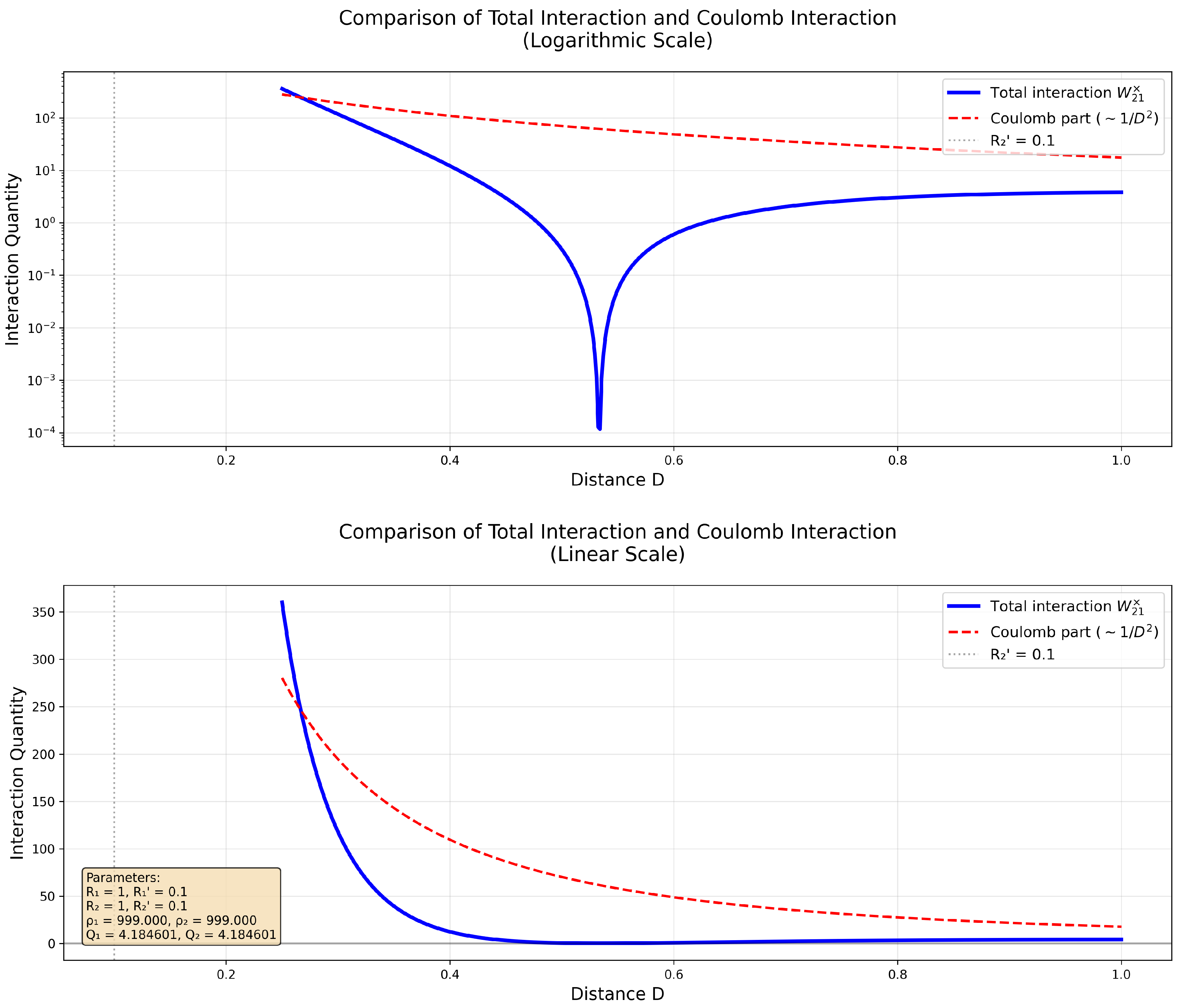
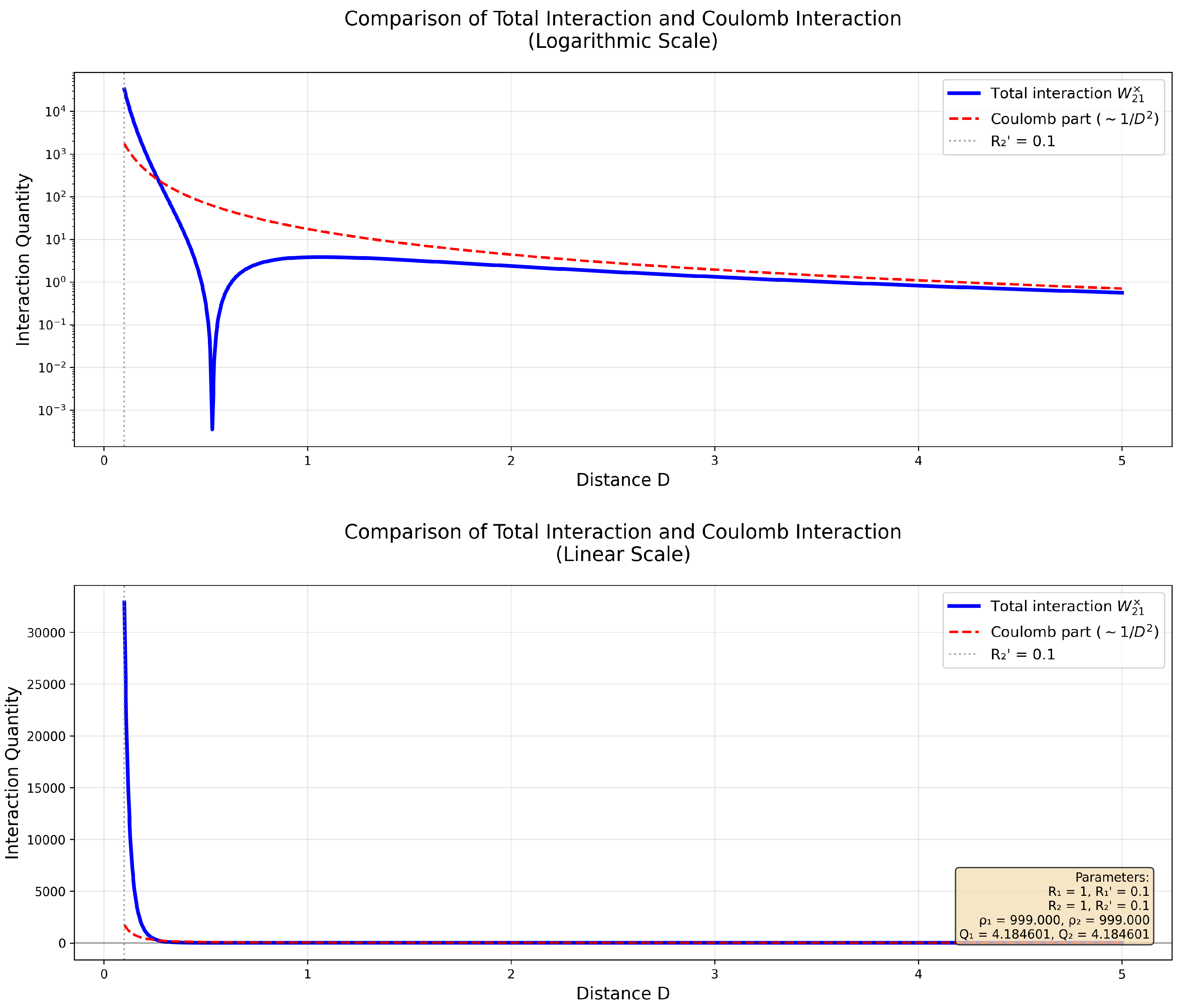
Figure 4. Visualization of the reduction in the amount of interaction at distances comparable to the sizes of an elementary charge (charge size 0.1 in conventional units, D range up to 5)

Figure 4. Visualization of the reduction in the amount of interaction at distances comparable to the sizes of an elementary charge (charge size 0.1 in conventional units, D range up to 5)

12.1. Final Understanding of the Energy Structure

Thus, the integral in our model not only provides the numerical value of the interaction but also splits the energy into three physical components:

• Self-energy of the clusters (vanishes);
• Real interaction of the two charges (cross term, Coulomb energy);
• Corrective terms for shielding and renormalization (ensure the physical adequacy of the field at small distances).

This structure allows for a rigorous derivation of the Lagrangian for a two-charge system from the geometry of 5D-space and the density distribution, without additional empirical postulates. Furthermore, the finite radii of the charges $R_1,R_2$ create a natural constraint $D>R$, which eliminates the problem of infinite energy and makes the model fully self-consistent.

13. Calculation of the Gradient Integral of the Cross-Term of Space Density Distribution

Analytical computation of the integral of the cross-term of the space density distribution is not feasible, but by applying the Ostrogradsky-Gauss theorem, one can compute the integral of the gradient, taking into account that the expression contains discontinuities due to the Heaviside functions in the expressions for $\Delta {\rho }_1$ and $\Delta {\rho }_2$.

Previously, we obtained that the cross-term of the total space density distribution is defined as the product of perturbations from two density clusters:

$$\Delta {\rho }_{\mathrm{cross}}\left({\mathbf{r}}_1\right)={\displaystyle \frac{1}{{\rho }_0}}\left[\Delta {\rho }_1\left({\mathbf{r}}_1\right)·\Delta {\rho }_2({\mathbf{r}}_1-\mathbf{D})\right],$$

where $\Delta {\rho }_1$ and $\Delta {\rho }_2$ are the density perturbations created by the first and second cluster, respectively, and ${\rho }_0$ is the reference (background) space density.

The analytical expressions for the perturbations are given via Heaviside functions and inverse fourth powers:

$$\Delta {\rho }_1\left({\mathbf{r}}_1\right)={\rho }_{1}H(R_1^{\prime }-r_1)-{\displaystyle \frac{{\rho }_1{R}_1^{\prime 4}}{3r_1^4}}H(r_1-R_1^{\prime }),$$

$$\Delta {\rho }_2({\mathbf{r}}_1-\mathbf{D})={\rho }_{2}H(R_2^{\prime }-|{\mathbf{r}}_1-\mathbf{D}\left|\right)-{\displaystyle \frac{{\rho }_2{R}_2^{\prime 4}}{3|{\mathbf{r}}_1{-\mathbf{D}|}^4}}H\left(\right|{\mathbf{r}}_1-\mathbf{D}|-R_2^{\prime }).$$

Thus,

$$\begin{array}{c}\Delta {\rho }_{\mathrm{cross}}\left({\mathbf{r}}_1\right)={\displaystyle \frac{1}{{\rho }_0}}\left[{\rho }_{1}H(R_1^{\prime }-r_1)-{\displaystyle \frac{{\rho }_1{R}_1^{\prime 4}}{3r_1^4}}H(r_1-R_1^{\prime })\right]\times \hfill \\ \hfill \left[{\rho }_{2}H(R_2^{\prime }-|{\mathbf{r}}_1-\mathbf{D}\left|\right)-{\displaystyle \frac{{\rho }_2{R}_2^{\prime 4}}{3|{\mathbf{r}}_1{-\mathbf{D}|}^4}}H\left(\right|{\mathbf{r}}_1-\mathbf{D}|-R_2^{\prime })\right].\end{array}$$

13.1. Integral of the Gradient of the Cross-Term and Application of the Ostrogradsky-Gauss Theorem

Consider the volume integral of the gradient of the cross-term over volume V:

$$\mathbf{F}:={\int }_V\nabla \Delta {\rho }_{\mathrm{cross}}\left({\mathbf{r}}_1\right)dV.$$

Since $\Delta {\rho }_{\mathrm{cross}}$ is a product of functions, each of which has a discontinuity (transition) on the spherical surface of radius $R_i^{\prime }$ (due to the Heaviside functions), the gradient $\nabla \Delta {\rho }_{\mathrm{cross}}$ contains a contribution concentrated on these surfaces.

For functions with compact support, the Ostrogradsky-Gauss theorem is applicable: the volume integral of the gradient of a function equals the flux of that function through the external boundary of the volume:

$$\mathbf{F}={\int }_V\nabla \Delta {\rho }_{\mathrm{cross}}dV={\oint }_{\partial V}\Delta {\rho }_{\mathrm{cross}}\mathbf{n}dS,$$

where $\partial V$ is the boundary of the integration volume, and $\mathbf{n}$ is the outward normal to $\partial V$.

13.2. Partitioning the Volume into Regions Accounting for Heaviside Discontinuities and Transition to the Sum over Surfaces $S_1$ and $S_2$

Since each of the functions $\Delta {\rho }_1$ and $\Delta {\rho }_2$ changes its analytical form precisely on the corresponding spherical surfaces $r_1=R_1^{\prime }$ and $|{\mathbf{r}}_1-\mathbf{D}|=R_2^{\prime }$, it is natural to partition the total volume V into subsets bounded by these surfaces. Denote $S_1$ and $S_2$ as the transition surfaces for the first and second Heaviside function, respectively.

Then the boundary of the combined volume containing all perturbation regions can be represented as the union of the internal surfaces where jumps occur and the possible external boundary at infinity (for compact support, the contribution at infinity is zero). Consequently, the flux through $\partial V$ reduces to the sum of fluxes through $S_1$ and $S_2$:

$$\mathbf{F}={\oint }_{\partial V}\Delta {\rho }_{\mathrm{cross}}\mathbf{n}dS={\oint }_{S_1}\Delta {\rho }_{\mathrm{cross}}{\mathbf{n}}_{1}d{S}_1+{\oint }_{S_2}\Delta {\rho }_{\mathrm{cross}}{\mathbf{n}}_{2}d{S}_2.$$

Reasons for the validity of this partitioning:

• Gradient Localization: Outside the regions where the Heaviside function changes (inside regions with constant analytical form), the function $\Delta {\rho }_{\mathrm{cross}}$ is smooth and contributes zero flux when considering a closed volume containing these regions; the essential contribution comes only from the transition on the discontinuity surfaces.
• Compact Support and Vanishing at the External Boundary: The original perturbations are defined such that beyond some finite radius they decay (or are zero in the sense of the Heaviside function and inverse powers when integrated over volume), so the flux through the external boundary at infinity is absent.
• Local Application of the Divergence Theorem: The Ostrogradsky-Gauss theorem can be applied piecewise to each of the simple volumes bounded by $S_1$ and $S_2$, and then the results are summed. Here, the orientations of the normals ${\mathbf{n}}_1$ and ${\mathbf{n}}_2$ are chosen as outward relative to the corresponding internal regions.
• Correctness for Possible Region Overlap: If the regions bounded by $S_1$ and $S_2$ intersect, the boundary of the union includes parts of both spheres and (if necessary) junction lines/areas; however, any internal part of the boundary common to two adjacent volumes is accounted for with opposite orientations and cancels out when summing the fluxes, and the remaining external parts give the total flux through $S_1$ and $S_2$.

Thus, we obtain the decomposition:

$$\begin{array}{|c|}\hline \mathbf{F}=I_{S_1}+I_{S_2},\\ \hline\end{array}$$

where

$$\begin{array}{cc}\hfill I_{S_1}& ={\oint }_{S_1}\Delta {\rho }_1\left({\mathbf{r}}_1\right)·\Delta {\rho }_2({\mathbf{r}}_1-\mathbf{D}){\mathbf{n}}_{1}d{S}_1,\hfill \\ \hfill I_{S_2}& ={\oint }_{S_2}\Delta {\rho }_1({\mathbf{r}}_2+\mathbf{D})·\Delta {\rho }_2\left({\mathbf{r}}_2\right){\mathbf{n}}_{2}d{S}_2.\hfill \end{array}$$

Substituting the expression for the cross-term $\Delta {\rho }_{\mathrm{cross}}={\displaystyle \frac{1}{{\rho }_0}}\Delta {\rho }_1·\Delta {\rho }_2$, we get:

$$\begin{array}{cc}{\int }_V\nabla \Delta {\rho }_{\mathrm{cross}}\left({\mathbf{r}}_1\right)dV={\displaystyle \frac{1}{{\rho }_0}}[{\oint }_{S_1}\Delta {\rho }_1\left({\mathbf{r}}_1\right)·\Delta {\rho }_2({\mathbf{r}}_1-\mathbf{D})·{\mathbf{n}}_{1}d{S}_1\hfill & \\ & \hfill +{\oint }_{S_2}\Delta {\rho }_1({\mathbf{r}}_2+\mathbf{D})·\Delta {\rho }_2\left({\mathbf{r}}_2\right)·{\mathbf{n}}_{2}d{S}_2].\end{array}$$

This expression represents the general form of the integral of the gradient of the cross-term of the space density through surface integrals dependent on the perturbations.

13.3. Consideration of the First Surface Integral $I_{S_1}$

Consider the first surface integral:

$$I_{S_1}={\oint }_{S_1}\Delta {\rho }_1\left({\mathbf{r}}_1\right)\Delta {\rho }_2({\mathbf{r}}_1-\mathbf{D}){\mathbf{n}}_{1}d{S}_1.$$

Substitute the analytical expressions for the density perturbations:

$$\Delta {\rho }_1\left({\mathbf{r}}_1\right)={\rho }_{1}H(R_1^{\prime }-r_1)-{\displaystyle \frac{{\rho }_1{R}_1^{\prime 4}}{3r_1^4}}H(r_1-R_1^{\prime }),$$

$$\Delta {\rho }_2({\mathbf{r}}_1-\mathbf{D})={\rho }_{2}H(R_2^{\prime }-|{\mathbf{r}}_1-\mathbf{D}\left|\right)-{\displaystyle \frac{{\rho }_2{R}_2^{\prime 4}}{3|{\mathbf{r}}_1{-\mathbf{D}|}^4}}H\left(\right|{\mathbf{r}}_1-\mathbf{D}|-R_2^{\prime }).$$

The product $\Delta {\rho }_1\Delta {\rho }_2$ contains four terms. After substitution into the integral we have:

$$\begin{array}{cc}\hfill I_{S_1}& =\underset{\left(1\right)}{\underbrace{{\rho }_1{\rho }_2{\oint }_{S_1}H(R_1^{\prime }-r_1)H(R_2^{\prime }-|{\mathbf{r}}_1-\mathbf{D}\left|\right){\mathbf{n}}_{1}d{S}_1}}\hfill \\ & -\underset{\left(2\right)}{\underbrace{{\displaystyle \frac{{\rho }_1{\rho }_2{R}_2^{\prime 4}}{3}}{\oint }_{S_1}H(R_1^{\prime }-r_1){\displaystyle \frac{H\left(\right|{\mathbf{r}}_1-\mathbf{D}|-R_2^{\prime })}{|{\mathbf{r}}_1{-\mathbf{D}|}^4}}{\mathbf{n}}_{1}d{S}_1}}\hfill \\ & -\underset{\left(3\right)}{\underbrace{{\displaystyle \frac{{\rho }_1{\rho }_2{R}_1^{\prime 4}}{3}}{\oint }_{S_1}{\displaystyle \frac{H(r_1-R_1^{\prime })H(R_2^{\prime }-|{\mathbf{r}}_1-\mathbf{D}\left|\right)}{r_1^4}}{\mathbf{n}}_{1}d{S}_1}}\hfill \\ & +\underset{\left(4\right)}{\underbrace{{\displaystyle \frac{{\rho }_1{\rho }_2{R}_1^{\prime 4}{R}_2^{\prime 4}}{9}}{\oint }_{S_1}{\displaystyle \frac{H(r_1-R_1^{\prime })H\left(\right|{\mathbf{r}}_1-\mathbf{D}|-R_2^{\prime })}{r_1^4{|{\mathbf{r}}_1-\mathbf{D}|}^4}}{\mathbf{n}}_{1}d{S}_1}}.\hfill \end{array}$$

Non-intersection Conditions

Assume that the spheres $S_1$ and $S_2$ do not intersect:

$$D>R_1^{\prime }+R_2^{\prime }.$$

Then:

• Term (1) on the surface $S_1$ is zero, since $H(R_2^{\prime }-|{\mathbf{r}}_1-\mathbf{D}\left|\right)=0$;
• Term (3) is also zero.

Only (2) and (4) remain:

$$\begin{array}{cc}\hfill I_{S_1}^{\left(2\right)}& =-{\displaystyle \frac{{\rho }_1{\rho }_2{R}_2^{\prime 4}}{3}}{\oint }_{S_1}H(R_1^{\prime }-r_1){\displaystyle \frac{H\left(\right|{\mathbf{r}}_1-\mathbf{D}|-R_2^{\prime })}{|{\mathbf{r}}_1{-\mathbf{D}|}^4}}{\mathbf{n}}_{1}d{S}_1,\hfill \\ \hfill I_{S_1}^{\left(4\right)}& ={\displaystyle \frac{{\rho }_1{\rho }_2{R}_1^{\prime 4}{R}_2^{\prime 4}}{9}}{\oint }_{S_1}{\displaystyle \frac{H(r_1-R_1^{\prime })H\left(\right|{\mathbf{r}}_1-\mathbf{D}|-R_2^{\prime })}{r_1^4{|{\mathbf{r}}_1-\mathbf{D}|}^4}}{\mathbf{n}}_{1}d{S}_1.\hfill \end{array}$$

Simplification on the Surface $S_1$

On the surface $S_1$ the radius is fixed ($r_1=R_1^{\prime }$) and the normal vector is radial:

$${\mathbf{n}}_1={\displaystyle \frac{{\mathbf{r}}_1}{R_1^{\prime }}}.$$

The Heaviside functions at the boundary take the value $H\left(0\right)=1/2$:

$$H(R_1^{\prime }-r_1)=H(r_1-R_1^{\prime })={\displaystyle \frac{1}{2}}.$$

Consequently, the integrals simplify:

$$I_{S_1}^{\left(2\right)}=-{\displaystyle \frac{{\rho }_1{\rho }_2{R}_2^{\prime 4}}{6}}{\oint }_{S_1}{\displaystyle \frac{H\left(\right|{\mathbf{r}}_1-\mathbf{D}|-R_2^{\prime })}{|{\mathbf{r}}_1{-\mathbf{D}|}^4}}{\mathbf{n}}_{1}d{S}_1,$$

$$I_{S_1}^{\left(4\right)}={\displaystyle \frac{{\rho }_1{\rho }_2{R}_2^{\prime 4}}{18}}{\oint }_{S_1}{\displaystyle \frac{H\left(\right|{\mathbf{r}}_1-\mathbf{D}|-R_2^{\prime })}{|{\mathbf{r}}_1{-\mathbf{D}|}^4}}{\mathbf{n}}_{1}d{S}_1.$$

Summation of Contributions

Summing the remaining terms, we obtain the final expression:

$$\begin{array}{|c|}\hline I_{S_1}=-{\displaystyle \frac{{\rho }_1{\rho }_2{R}_2^{\prime 4}}{9}}{\oint }_{S_1}{\displaystyle \frac{H\left(\right|{\mathbf{r}}_1-\mathbf{D}|-R_2^{\prime })}{|{\mathbf{r}}_1{-\mathbf{D}|}^4}}{\mathbf{n}}_{1}d{S}_1.\\ \hline\end{array}$$

13.4. Consideration of the Second Surface Integral $I_{S_2}$

Consider the second surface integral:

$$I_{S_2}={\oint }_{S_2}\Delta {\rho }_1\left({\mathbf{r}}_1\right)\Delta {\rho }_2({\mathbf{r}}_1-\mathbf{D}){\mathbf{n}}_2\left({\mathbf{r}}_1\right)d{S}_2.$$

The surface $S_2$ in the ${\mathbf{r}}_1$ system is given by:

$$S_2:|{\mathbf{r}}_1-\mathbf{D}|=R_2^{\prime },$$

and the condition of non-intersecting spheres is satisfied:

$$|{\mathbf{r}}_1-\mathbf{D}|>R_1^{\prime },D>R_1^{\prime }+R_2^{\prime }.$$

Substitute the analytical expressions for the perturbations:

$$\Delta {\rho }_1\left({\mathbf{r}}_1\right)={\rho }_{1}H(R_1^{\prime }-r_1)-{\displaystyle \frac{{\rho }_1{R}_1^{\prime 4}}{3r_1^4}}H(r_1-R_1^{\prime }),$$

$$\Delta {\rho }_2({\mathbf{r}}_1-\mathbf{D})={\rho }_{2}H(R_2^{\prime }-|{\mathbf{r}}_1-\mathbf{D}\left|\right)-{\displaystyle \frac{{\rho }_2{R}_2^{\prime 4}}{3|{\mathbf{r}}_1{-\mathbf{D}|}^4}}H\left(\right|{\mathbf{r}}_1-\mathbf{D}|-R_2^{\prime }).$$

Expanding the product, we obtain four terms:

$$\begin{array}{c}{I}_{S_2}=\underset{\left(1\right)}{\underbrace{{\rho }_1{\rho }_2{\oint }_{S_2}H(R_1^{\prime }-r_1)H(R_2^{\prime }-|{\mathbf{r}}_1-\mathbf{D}\left|\right){\mathbf{n}}_{2}d{S}_2}}\hfill \\ \hspace{1em}\hspace{1em}\hspace{1em}\hspace{1em}-\underset{\left(2\right)}{\underbrace{{\displaystyle \frac{{\rho }_1{\rho }_2{R}_2^{\prime 4}}{3}}{\oint }_{S_2}H(R_1^{\prime }-r_1){\displaystyle \frac{H\left(\right|{\mathbf{r}}_1-\mathbf{D}|-R_2^{\prime })}{|{\mathbf{r}}_1{-\mathbf{D}|}^4}}{\mathbf{n}}_{2}d{S}_2}}\\ \hspace{1em}\hspace{1em}\hspace{1em}\hspace{1em}-\underset{\left(3\right)}{\underbrace{{\displaystyle \frac{{\rho }_1{\rho }_2{R}_1^{\prime 4}}{3}}{\oint }_{S_2}{\displaystyle \frac{H(r_1-R_1^{\prime })H(R_2^{\prime }-|{\mathbf{r}}_1-\mathbf{D}\left|\right)}{r_1^4}}{\mathbf{n}}_{2}d{S}_2}}\\ \hfill \hspace{1em}\hspace{1em}\hspace{1em}\hspace{1em}\hspace{1em}\hspace{1em}\hspace{1em}\hspace{1em}\hspace{1em}\hspace{1em}\hspace{1em}\hspace{1em}+\underset{\left(4\right)}{\underbrace{{\displaystyle \frac{{\rho }_1{\rho }_2{R}_1^{\prime 4}{R}_2^{\prime 4}}{9}}{\oint }_{S_2}{\displaystyle \frac{H(r_1-R_1^{\prime })H\left(\right|{\mathbf{r}}_1-\mathbf{D}|-R_2^{\prime })}{r_1^4{|{\mathbf{r}}_1-\mathbf{D}|}^4}}{\mathbf{n}}_{2}d{S}_2}}.\end{array}$$

13.4.1. Transition to the ${\mathbf{r}}_2$ System

Make the variable change:

$${\mathbf{r}}_1={\mathbf{r}}_2+\mathbf{D}.$$

In the new system the surface $S_2$ has a simple form:

$$S_2:\left|{\mathbf{r}}_2\right|=R_2^{\prime },{\mathbf{n}}_2={\displaystyle \frac{{\mathbf{r}}_2}{R_2^{\prime }}},d{S}_2=R_2^{\prime 2}\sin {\theta }_{2}d{\theta }_{2}d{\varphi }_2.$$

The product of Heaviside functions and power terms is rewritten in terms of ${\mathbf{r}}_2$:

$$\begin{array}{cc}\hfill \left(1\right)& ={\rho }_1{\rho }_2{\oint }_{S_2}H(R_1^{\prime }-|{\mathbf{r}}_2+\mathbf{D}\left|\right)H(R_2^{\prime }-r_2){\mathbf{n}}_{2}d{S}_2,\hfill \\ \hfill \left(2\right)& =-{\displaystyle \frac{{\rho }_1{\rho }_2{R}_2^{\prime 4}}{3}}{\oint }_{S_2}H(R_1^{\prime }-|{\mathbf{r}}_2+\mathbf{D}\left|\right){\displaystyle \frac{H(r_2-R_2^{\prime })}{r_2^4}}{\mathbf{n}}_{2}d{S}_2,\hfill \\ \hfill \left(3\right)& =-{\displaystyle \frac{{\rho }_1{\rho }_2{R}_1^{\prime 4}}{3}}{\oint }_{S_2}{\displaystyle \frac{H\left(\right|{\mathbf{r}}_2+\mathbf{D}|-R_1^{\prime })H(R_2^{\prime }-r_2)}{|{\mathbf{r}}_2{+\mathbf{D}|}^4}}{\mathbf{n}}_{2}d{S}_2,\hfill \\ \hfill \left(4\right)& ={\displaystyle \frac{{\rho }_1{\rho }_2{R}_1^{\prime 4}{R}_2^{\prime 4}}{9}}{\oint }_{S_2}{\displaystyle \frac{H\left(\right|{\mathbf{r}}_2+\mathbf{D}|-R_1^{\prime })H(r_2-R_2^{\prime })}{|{\mathbf{r}}_2{+\mathbf{D}|}^4{r}_2^4}}{\mathbf{n}}_{2}d{S}_2.\hfill \end{array}$$

13.4.2. Discarding Zero Terms

Using the condition of non-intersecting spheres ($D>R_1^{\prime }+R_2^{\prime }$) and the values of the Heaviside function at the boundary ($r_2=R_2^{\prime }$), $H\left(0\right)=1/2$:

• $\left(1\right)=0$, since there is no overlap region;
• $\left(2\right)$ is symmetric with respect to the center of $S_2$ and gives zero vector flux;
• $\left(3\right)$ and $\left(4\right)$ remain, which depend on $|{\mathbf{r}}_2+\mathbf{D}|$ and give non-zero contributions.

13.4.3. Final Form of the Integral $I_{S_2}$

Summing the remaining terms and taking into account the factor of $1/2$ from the Heaviside function at the boundary:

$$\begin{array}{|c|}\hline I_{S_2}=-{\displaystyle \frac{{\rho }_1{\rho }_2{R}_1^{\prime 4}}{9}}{\oint }_{S_2}{\displaystyle \frac{H\left(\right|{\mathbf{r}}_2+\mathbf{D}|-R_1^{\prime })}{|{\mathbf{r}}_2{+\mathbf{D}|}^4}}{\mathbf{n}}_{2}d{S}_2.\\ \hline\end{array}$$

The surface $S_2$ in the ${\mathbf{r}}_2$ system is given by the equation $|{\mathbf{r}}_2|=R_2^{\prime }$, and the normal is directed radially outward: ${\mathbf{n}}_2={\mathbf{r}}_2/R_2^{\prime }$.

13.5. Evaluation of Integrals $I_{S_1}$ and $I_{S_2}$

13.5.1. 1. Integral $I_{S_1}$

For non-intersecting spheres ($D>R_1^{\prime }+R_2^{\prime }$), after accounting for all Heaviside terms, the remaining integral is:

$$I_{S_1}=-{\displaystyle \frac{{\rho }_1{\rho }_2{R}_2^{\prime 4}}{9}}{\oint }_{S_1}{\displaystyle \frac{{\mathbf{n}}_1}{|{\mathbf{r}}_1{-\mathbf{D}|}^4}}d{S}_1,$$

where the surface $S_1$ is defined by the radius $r_1=R_1^{\prime }$, and the normal vector points radially outward:

$${\mathbf{n}}_1={\displaystyle \frac{{\mathbf{r}}_1}{R_1^{\prime }}},d{S}_1=R_1^{\prime 2}\sin {\theta }_{1}d{\theta }_{1}d{\varphi }_1.$$

Substituting spherical coordinates:

$${\mathbf{r}}_1=R_1^{\prime }(\sin {\theta }_1\cos {\varphi }_1,\sin {\theta }_1\sin {\varphi }_1,\cos {\theta }_1),$$

the integral becomes:

$$I_{S_1}=-{\displaystyle \frac{{\rho }_1{\rho }_2{R}_2^{\prime 4}{R}_1^{\prime 2}}{9}}{\int }_0^{\pi }{\int }_0^{2\pi }{\displaystyle \frac{(\sin {\theta }_1\cos {\varphi }_1,\sin {\theta }_1\sin {\varphi }_1,\cos {\theta }_1)\sin {\theta }_{1}d{\varphi }_{1}d{\theta }_1}{{(R_1^{\prime 2}+D^2-2R_1^{\prime }D\cos {\theta }_1)}^2}}.$$

Integration over ${\varphi }_1$ nullifies the x- and y-components, leaving only the z-component:

$${\left(I_{S_1}\right)}_z=-{\displaystyle \frac{2\pi {\rho }_1{\rho }_2{R}_2^{\prime 4}{R}_1^{\prime 2}}{9}}{\int }_0^{\pi }{\displaystyle \frac{\cos {\theta }_1\sin {\theta }_{1}d{\theta }_1}{{(R_1^{\prime 2}+D^2-2R_1^{\prime }D\cos {\theta }_1)}^2}}.$$

Introducing the substitution $u=\cos {\theta }_1$, $du=-\sin {\theta }_{1}d{\theta }_1$:

$${\left(I_{S_1}\right)}_z=-{\displaystyle \frac{2\pi {\rho }_1{\rho }_2{R}_2^{\prime 4}{R}_1^{\prime 2}}{9}}{\int }_{-1}^1{\displaystyle \frac{udu}{{(R_1^{\prime 2}+D^2-2R_1^{\prime }Du)}^2}}.$$

Using the standard antiderivative:

$$\int {\displaystyle \frac{udu}{{(a-bu)}^2}}=-{\displaystyle \frac{u}{b(a-bu)}}-{\displaystyle \frac{1}{b^2}}\ln (a-bu),a=R_1^{\prime 2}+D^2,b=2R_1^{\prime }D.$$

Substituting the limits $u=-1$ and $u=1$ yields:

$${\int }_{-1}^1{\displaystyle \frac{udu}{{(R_1^{\prime 2}+D^2-2R_1^{\prime }Du)}^2}}=-{\displaystyle \frac{R_1^{\prime 2}+D^2}{R_1^{\prime }D{(D^2-R_1^{\prime 2})}^2}}+{\displaystyle \frac{1}{4R_1^{\prime 2}{D}^2}}\ln {\displaystyle \frac{{(R_1^{\prime }-D)}^2}{{(R_1^{\prime }+D)}^2}}.$$

Removing the modulus under the logarithm, considering $D>R_1^{\prime }$, we obtain the complex branch:

$$2\ln (R_1^{\prime }-D)=2\ln (D-R_1^{\prime })+i2\pi .$$

Final form of the integral $I_{S_1}$:

$$\begin{array}{|c|}\hline I_{S_1}=-{\displaystyle \frac{2\pi {\rho }_1{\rho }_2{R}_2^{\prime 4}{R}_1^{\prime 2}}{9}}\left[-{\displaystyle \frac{R_1^{\prime 2}+D^2}{R_1^{\prime }D{(D^2-R_1^{\prime 2})}^2}}+{\displaystyle \frac{1}{4R_1^{\prime 2}{D}^2}}\left(\ln {\displaystyle \frac{D-R_1^{\prime }}{R_1^{\prime }+D}}+i2\pi \right)\right]{\mathbf{e}}_z.\\ \hline\end{array}$$

13.5.2. 2. Integral $I_{S_2}$

After substituting the radius $r_2=R_2^{\prime }$ and the normal ${\mathbf{n}}_2={\mathbf{r}}_2/R_2^{\prime }$, the integral becomes:

$$I_{S_2}={\displaystyle \frac{2\pi {\rho }_1{\rho }_2{R}_1^{\prime 4}{R}_2^{\prime 2}}{9}}{\int }_0^{\pi }{\displaystyle \frac{\cos {\theta }_2\sin {\theta }_{2}d{\theta }_2}{{(R_2^{\prime 2}+D^2+2R_2^{\prime }D\cos {\theta }_2)}^2}}{\mathbf{e}}_z.$$

Introducing $u=\cos {\theta }_2$, $du=-\sin {\theta }_{2}d{\theta }_2$, changing the integration limits ($u=1\to u=-1$):

$$I_{S_2}={\displaystyle \frac{2\pi {\rho }_1{\rho }_2{R}_1^{\prime 4}{R}_2^{\prime 2}}{9}}{\int }_{-1}^1{\displaystyle \frac{udu}{{(R_2^{\prime 2}+D^2-2R_2^{\prime }Du)}^2}}{\mathbf{e}}_z.$$

Substituting the limits and removing the modulus considering $D>R_2^{\prime }$ gives the complex branch:

$$2\ln (R_2^{\prime }-D)=2\ln (D-R_2^{\prime })+i2\pi .$$

Final expression for the integral $I_{S_2}$:

$$\begin{array}{|c|}\hline I_{S_2}={\displaystyle \frac{2\pi {\rho }_1{\rho }_2{R}_1^{\prime 4}{R}_2^{\prime 2}}{9}}\left[-{\displaystyle \frac{R_2^{\prime 2}+D^2}{R_2^{\prime }D{(D^2-R_2^{\prime 2})}^2}}+{\displaystyle \frac{1}{4R_2^{\prime 2}{D}^2}}\left(\ln {\displaystyle \frac{D-R_2^{\prime }}{R_2^{\prime }+D}}+i2\pi \right)\right]{\mathbf{e}}_z.\\ \hline\end{array}$$

13.6. Final Expression for $\Delta {\rho }_{\mathrm{cross}}$

Taking into account the computed surface integrals $I_{S_1}$ and $I_{S_2}$, the cross term of the total space density distribution in a system of two non-intersecting spheres ($D>R_1^{\prime }+R_2^{\prime }$) can be written as:

$$\Delta {\rho }_{\mathrm{cross}}\approx {\displaystyle \frac{1}{{\rho }_0}}\left(I_{S_1}+I_{S_2}\right).$$

Substituting the obtained integrals, we have:

$$\begin{array}{c}\Delta {\rho }_{\mathrm{cross}}=-{\displaystyle \frac{2\pi {\rho }_1{\rho }_2{R}_2^{\prime 4}{R}_1^{\prime 2}}{9{\rho }_0}}\left[-{\displaystyle \frac{R_1^{\prime 2}+D^2}{R_1^{\prime }D{(D^2-R_1^{\prime 2})}^2}}+{\displaystyle \frac{1}{4R_1^{\prime 2}{D}^2}}\left(\ln {\displaystyle \frac{D-R_1^{\prime }}{R_1^{\prime }+D}}+i2\pi \right)\right]{\mathbf{e}}_z\hfill \\ \hfill +{\displaystyle \frac{2\pi {\rho }_1{\rho }_2{R}_1^{\prime 4}{R}_2^{\prime 2}}{9{\rho }_0}}\left[-{\displaystyle \frac{R_2^{\prime 2}+D^2}{R_2^{\prime }D{(D^2-R_2^{\prime 2})}^2}}+{\displaystyle \frac{1}{4R_2^{\prime 2}{D}^2}}\left(\ln {\displaystyle \frac{D-R_2^{\prime }}{R_2^{\prime }+D}}+i2\pi \right)\right]{\mathbf{e}}_z.\end{array}$$

Comments:

• The first term $I_{S_1}$ corresponds to the flux contribution through the surface of the first density cluster $S_1$; its direction is given by the sphere’s normal and points along the axis connecting the cluster centers ${\mathbf{e}}_z$.
• The second term $I_{S_2}$ reflects the flux through the surface of the second cluster $S_2$, also along ${\mathbf{e}}_z$.
• Both integrals contain a complex logarithmic term $i2\pi$, which reflects the branching of the solution and the imaginary nature of space energy density.
• The sign of each integral indicates the direction of the corresponding force; in magnitude $|I_{S_1}|=|I_{S_2}|$ when $R_1^{\prime }=R_2^{\prime }$ and ${\rho }_1={\rho }_2$, and the directions are opposite, as is characteristic of Coulomb-like interaction.
• The sum $I_{S_1}+I_{S_2}$ gives the total cross contribution $\Delta {\rho }_{\mathrm{cross}}$ to the space density distribution and corresponds to the force acting on each cluster.

13.7. Complex Part of the Cross Integral

Let us extract only the imaginary parts of the integrals $I_{S_1}$ and $I_{S_2}$, taking into account all factors before $i2\pi$ and ${\rho }_0$ in the denominator:

$$\begin{array}{cc}\hfill \Im \left(I_{S_1}\right)& =-{\displaystyle \frac{2\pi {\rho }_1{\rho }_2{R}_2^{\prime 4}{R}_1^{\prime 2}}{9{\rho }_0}}·{\displaystyle \frac{i2\pi }{4R_1^{\prime 2}{D}^2}}{\mathbf{e}}_z=-i{\displaystyle \frac{{\pi }^2{\rho }_1{\rho }_2{R}_2^{\prime 4}}{9{\rho }_0{D}^2}}{\mathbf{e}}_z,\hfill \\ \hfill \Im \left(I_{S_2}\right)& ={\displaystyle \frac{2\pi {\rho }_1{\rho }_2{R}_1^{\prime 4}{R}_2^{\prime 2}}{9{\rho }_0}}·{\displaystyle \frac{i2\pi }{4R_2^{\prime 2}{D}^2}}{\mathbf{e}}_z=i{\displaystyle \frac{{\pi }^2{\rho }_1{\rho }_2{R}_1^{\prime 4}}{9{\rho }_0{D}^2}}{\mathbf{e}}_z.\hfill \end{array}$$

13.7.0.2. Comments:

• The complex part of the integrals reflects the imaginary nature of the space energy density.
• The magnitudes of these vectors coincide when $R_1^{\prime }=R_2^{\prime }$, but their directions are opposite (${\mathbf{e}}_z$ and $-{\mathbf{e}}_z$).
• The sum of the imaginary parts $I_{S_1}+I_{S_2}$ corresponds to the imaginary component of the cross force acting on both clusters.

13.8. Potential Energy of Clusters via the Imaginary Part of the Cross Integral

Note that the integral of the imaginary part of the cross integral over the vector $\mathbf{D}$ from the current position to infinity gives the scalar potential energy of each cluster. Denote it as $U_1$ and $U_2$ for the first and second cluster, respectively.

Taking into account ${\rho }_0$ in the denominator and the found complex parts:

$$\Im \left(I_{S_1}\right)=-i{\displaystyle \frac{{\pi }^2{\rho }_1{\rho }_2{R}_2^{\prime 4}}{9{\rho }_0{D}^2}}{\mathbf{e}}_z,\Im \left(I_{S_2}\right)=i{\displaystyle \frac{{\pi }^2{\rho }_1{\rho }_2{R}_1^{\prime 4}}{9{\rho }_0{D}^2}}{\mathbf{e}}_z.$$

The potential energy of each cluster is defined as the integral of the force over the vector $\mathbf{D}$ from D to infinity:

$$U_1={\int }_D^{\infty }\Im \left(I_{S_1}\right)·d\mathbf{D}=-i{\displaystyle \frac{{\pi }^2{\rho }_1{\rho }_2{R}_2^{\prime 4}}{9{\rho }_0}}{\int }_D^{\infty }{\displaystyle \frac{dD}{D^2}},$$

$$U_2={\int }_D^{\infty }\Im \left(I_{S_2}\right)·d\mathbf{D}=i{\displaystyle \frac{{\pi }^2{\rho }_1{\rho }_2{R}_1^{\prime 4}}{9{\rho }_0}}{\int }_D^{\infty }{\displaystyle \frac{dD}{D^2}}.$$

Computing the standard integral ${\int }_D^{\infty }{D}^{-2}dD={\displaystyle \frac{1}{D}}$, we obtain the final expressions:

$$\begin{array}{|c|}\hline U_1=-i{\displaystyle \frac{{\pi }^2{\rho }_1{\rho }_2{R}_2^{\prime 4}}{9{\rho }_{0}D}},U_2=i{\displaystyle \frac{{\pi }^2{\rho }_1{\rho }_2{R}_1^{\prime 4}}{9{\rho }_{0}D}}.\\ \hline\end{array}$$

13.9. Potentials of Clusters via the Imaginary Part of the Cross Integral

To determine the electric field potential from each cluster, we use the found imaginary energies $U_1$ and $U_2$, considering that the potential is the ratio of energy to the "charge" on which the field acts. In our theory, the "charge" corresponds to the density ${\rho }_1$ or ${\rho }_2$. Multiplying by the coefficient $12/\pi$, we obtain:

$${\Phi }_2={\displaystyle \frac{12}{\pi {\rho }_1}}{U}_1=-i{\displaystyle \frac{12}{\pi {\rho }_1}}·{\displaystyle \frac{{\pi }^2{\rho }_1{\rho }_2{R}_2^{\prime 4}}{9{\rho }_{0}D}}=-i{\displaystyle \frac{4\pi {\rho }_2{R}_2^{\prime 4}}{3{\rho }_{0}D}},$$

$${\Phi }_1={\displaystyle \frac{12}{\pi {\rho }_2}}{U}_2=i{\displaystyle \frac{12}{\pi {\rho }_2}}·{\displaystyle \frac{{\pi }^2{\rho }_1{\rho }_2{R}_1^{\prime 4}}{9{\rho }_{0}D}}=i{\displaystyle \frac{4\pi {\rho }_1{R}_1^{\prime 4}}{3{\rho }_{0}D}}.$$

14. Relationship Between the Calculation of the Total Disturbance Quantity of Space Density in 5D and the Solution of the Gradient Integral of Space Density in 3D

The quadratic part $\left(W_{\mathrm{cross}}\right)$ represents precisely that component of the total energy of the system of two density clusters which in the Lagrangian corresponds to the energy of the electric field — the very part that in classical electrodynamics is expressed through the integral of the square of the sum of field intensities:

$$W_{\mathrm{field}}\propto \int {({\mathbf{E}}_1+{\mathbf{E}}_2)}^{2}dV=\int {\mathbf{E}}_1^{2}dV+\int {\mathbf{E}}_2^{2}dV+2\int {\mathbf{E}}_1·{\mathbf{E}}_{2}dV.$$

The cross term $2\int {\mathbf{E}}_1·{\mathbf{E}}_{2}dV$ determines the interaction energy between the two sources and it is this term that plays the role of the physical analogue of $W_{\mathrm{cross}}$ in the proposed model.

In the expression for the total energy:

$$\begin{array}{cc}\hfill W_{\mathrm{total}}& =\left({\displaystyle \frac{8}{15}}{\displaystyle \frac{Q_1{R}_1^2}{D^2}}-{\displaystyle \frac{Q_1{R}_1}{D}}\right)+\left(-{\displaystyle \frac{8}{15}}{\displaystyle \frac{Q_2{R}_2^2}{D^2}}+{\displaystyle \frac{Q_2{R}_2}{D}}\right)\hfill \\ & +{\displaystyle \frac{1}{{\rho }_0}}\left({\displaystyle \frac{64}{225}}{\displaystyle \frac{Q_1{Q}_2{R}_1^2{R}_2^2}{D^4}}-{\displaystyle \frac{8}{15}}{\displaystyle \frac{Q_1{Q}_2{R}_1^2{R}_2}{D^3}}-{\displaystyle \frac{8}{15}}{\displaystyle \frac{Q_1{Q}_2{R}_1{R}_2^2}{D^3}}+{\displaystyle \frac{Q_1{Q}_2{R}_1{R}_2}{D^2}}\right),\hfill \end{array}$$

the second line, proportional to $(1/{\rho }_0)$, is exactly the cross part $W_{\mathrm{cross}}$, describing the interaction energy. Its last term, decaying as $1/D^2$, is dominant at large distances and represents the analogue of Coulomb interaction between two "charges" — the density clusters of space.

Connection with the Three-Dimensional Gradient Integral

In the three-dimensional analysis based on the integral of the gradient of the cross density term, surface integrals $I_{S_1}$ and $I_{S_2}$ were obtained, whose imaginary parts describe the vector forces acting on each cluster. Integrating these forces along the direction $\mathbf{D}$ allowed us to obtain expressions for the imaginary potential energies $U_1$ and $U_2$, from which the field potentials ${\Phi }_1$ and ${\Phi }_2$ were determined.

If we consider the product of the potentials, adjusted for the background space density, then the expression

$${\rho }_0{\Phi }_1{\Phi }_2$$

exactly reproduces the last, Coulomb-like term in $W_{\mathrm{cross}}$. This shows that to maintain the dimensionality of energy and the physical interpretation of the field, it is necessary to account for the factor ${\rho }_0$, analogous to ${\epsilon }_0$ in classical electrodynamics, where the field energy is defined as

$$W_{\mathrm{field}}={\displaystyle \frac{{\epsilon }_0}{2}}\int E^{2}dV.$$

14.0.1. Physical Interpretation

1. **Equivalence of Potentials and Field Energy.** The product ${\rho }_0{\Phi }_1{\Phi }_2$ expresses the interacting part of the field energy, similar to how in classical theory the interaction energy of two charges is expressed through ${\epsilon }_0{E}_1{E}_2$. This confirms that the potential computed via the imaginary part of the density distribution is indeed a physical analogue of the electric potential.

2. **Imaginary Nature of Space Energy Density.** The appearance of the imaginary unit in the solution indicates that the vacuum energy density has an imaginary component, projecting into our three-dimensional space from a higher (5D) structure. Thus, electromagnetic interaction can be viewed as a three-dimensional projection of a multidimensional exchange of space density.

3. **Consistency of 3D and 5D Solutions.** The structure of the terms, their dependencies on $R_i$, $Q_i$, and D, as well as the common factor $(1/{\rho }_0)$ demonstrate an exact correspondence between the results obtained in the three-dimensional and five-dimensional analyses. This shows that the three-dimensional solution via the imaginary part of the field not only agrees but fully reproduces the multidimensional structure of the interaction.

The obtained equality

$$W_{\mathrm{cross}}\sim {\rho }_0{\Phi }_1{\Phi }_2$$

demonstrates a deep connection between the three-dimensional description of the field via potentials and the five-dimensional form of the total energy of the system. This confirms that electromagnetic interaction in our space is a manifestation of a more fundamental multidimensional dynamics of space density, and the background density ${\rho }_0$ serves as a universal "coupling constant" between the geometry of space and its energy content.

15. Dimensional Analysis of Space Density – A Hypothetical Non-Geometric “Dimension” of Space

Potential Energy of the First Charge at Minimum Distance Between Clusters

Consider the expression for the potential energy of the first cluster $U_1$, obtained earlier via the integral of the gradient of the imaginary part of the cross-term density distribution. Substitute the minimum allowable distance between the centers of the density clusters, which in this formulation is taken as

$$D=2R_2^{\prime }.$$

This corresponds to the situation adopted when calculating contributions using Heaviside functions (the boundary of the second cluster is located at a distance $2R_2^{\prime }$ from the center of the first cluster in the considered configuration).

Substitution of the Expression for Charge $Q_2$

The charge of the second cluster is expressed through its density and radius as

$$Q_2={\displaystyle \frac{4}{3}}\pi {\rho }_2{R}_2^{\prime 3}.$$

The original expression for $U_1$ before substituting D is

$$U_1={\displaystyle \frac{{\pi }^2{\rho }_1{\rho }_2{R}_2^{\prime 4}i}{9{\rho }_{0}D}}.$$

Substituting $D=2R_2^{\prime }$, we get

$$U_1={\displaystyle \frac{{\pi }^2{\rho }_1{\rho }_2{R}_2^{\prime 4}i}{9{\rho }_0\left(2R_2^{\prime }\right)}}={\displaystyle \frac{{\pi }^2{\rho }_1{\rho }_2{R}_2^{\prime 3}i}{18{\rho }_0}}.$$

To isolate the dependence on the total "charge" of the second cluster, express ${\rho }_2{R}_2^{\prime 3}$ in terms of $Q_2$:

$${\rho }_2{R}_2^{\prime 3}={\displaystyle \frac{3Q_2}{4\pi }}.$$

Substituting this into the expression for $U_1$, we obtain

$$U_1={\displaystyle \frac{{\pi }^2{\rho }_1}{18{\rho }_0}}·{\displaystyle \frac{3Q_2}{4\pi }}i={\displaystyle \frac{\pi {\rho }_1{Q}_{2}i}{24{\rho }_0}}.$$

Replacing Charge $Q_2$ via Volume and Background Space Density

By definition, the charge $Q_2$ can be written as the change in the background space density over the corresponding volume:

$$Q_2={\rho }_0\left(V\left(R_2\right)-V\left(R_2^{\prime }\right)\right),V\left(R\right)={\displaystyle \frac{4}{3}}\pi R^3.$$

Substitute this into the expression for $U_1$:

$$U_1={\displaystyle \frac{\pi {\rho }_{1}i}{24{\rho }_0}}·{\rho }_0\left[{\displaystyle \frac{4}{3}}\pi (R_2^3-R_2^{\prime 3})\right].$$

Canceling ${\rho }_0$, we get

$$U_1={\displaystyle \frac{\pi {\rho }_{1}i}{24}}·{\displaystyle \frac{4}{3}}\pi (R_2^3-R_2^{\prime 3})={\displaystyle \frac{{\pi }^2{\rho }_{1}i}{18}}(R_2^3-R_2^{\prime 3}).$$

Thus, the final expression for the potential energy of the first cluster at $D=2R_2^{\prime }$ is:

$$\begin{array}{|c|}\hline U_1={\displaystyle \frac{{\pi }^2{\rho }_{1}i}{18}}(R_2^3-R_2^{\prime 3}).\\ \hline\end{array}$$

If in a specific problem $R_2$ is considered the outer radius of the second cluster, then the volume difference gives the quantity used above.

Dimensional Analysis

1. Potential energy $U_1$ has the dimension of energy:

$$\left[U_1\right]={\mathrm{ML}}^2{\mathrm{T}}^{-2}.$$

2. The volume difference $(R_2^3-R_2^{\prime 3})$ has the dimension ${\mathrm{L}}^3$.

3. From the relation

$$U_1=i{\displaystyle \frac{{\pi }^2{\rho }_1}{18}}(R_2^3-R_2^{\prime 3})$$

we obtain for the factor preceding the volume:

$$\left[i{\rho }_1\right]·{\mathrm{L}}^3={\mathrm{ML}}^2{\mathrm{T}}^{-2},$$

whence

$$\left[i{\rho }_1\right]={\mathrm{ML}}^{-1}{\mathrm{T}}^{-2}.$$

4. Consequently, the imaginary space density ${\rho }_1$ has the dimension:

$$\begin{array}{|c|}\hline \left[{\rho }_1\right]={\mathrm{ML}}^{-1}{\mathrm{T}}^{-2}\\ \hline\end{array}.$$

The imaginary unit i in this relation does not change the numerical dimension but marks that the quantity ${\rho }_1$ is written in complex form; the space density itself is treated as a hypothetical (non-geometric) property present in both 3D and 5D.

Substitution of Imaginary Densities and Return to Real Force

Take the original expression for the vector force (imaginary part) acting on the first cluster:

$${\mathbf{F}}_1=-i{\displaystyle \frac{2{\pi }^2{\rho }_1{\rho }_2{R}_2^{\prime 4}}{9{\rho }_0{D}^2}}{\mathbf{e}}_D,$$

where ${\mathbf{e}}_D$ is the unit vector along the direction $\mathbf{D}$.

Introduce the representation of imaginary densities via real quantities (${\rho }^{\mathrm{real}}$):

$${\rho }_1=-i{\rho }_1^{\mathrm{real}},{\rho }_2=-i{\rho }_2^{\mathrm{real}},{\rho }_0=-i{\rho }_0^{\mathrm{real}}.$$

Substitute these notations:

$${\mathbf{F}}_1=-i{\displaystyle \frac{2{\pi }^2(-i{\rho }_1^{\mathrm{real}})(-i{\rho }_2^{\mathrm{real}})R_2^{\prime 4}}{9(-i{\rho }_0^{\mathrm{real}})D^2}}{\mathbf{e}}_D.$$

Calculating the product of imaginary factors:

• In the numerator: $(-i)·(-i)=-1$, hence $(-i{\rho }_1^{\mathrm{real}})(-i{\rho }_2^{\mathrm{real}})=-{\rho }_1^{\mathrm{real}}{\rho }_2^{\mathrm{real}}$.
• Considering the external factor $-i$, we get i in the numerator.
• In the denominator $(-i)$ from ${\rho }_0$.

The fraction in terms of imaginary factors:

$${\displaystyle \frac{i}{-i}}=-1.$$

Consequently, the force becomes real:

$$\begin{array}{|c|}\hline {\mathbf{F}}_1=-{\displaystyle \frac{2{\pi }^2{\rho }_1^{\mathrm{real}}{\rho }_2^{\mathrm{real}}{R}_2^{\prime 4}}{9{\rho }_0^{\mathrm{real}}{D}^2}}{\mathbf{e}}_D.\\ \hline\end{array}$$

Substituting $D=2R_2^{\prime }$, the numerical coefficient adjusts accordingly, leaving the force real and with the correct "minus" sign, as for a Coulomb-type interaction.

16. Derivation of the Equation for Magnetic Interaction of Two Moving Charges: Theoretical Derivation of the Biot-Savart Law

Let two clusters move with velocities ${\mathbf{V}}_1$ and ${\mathbf{V}}_2$, and their density cluster "radii" be equal: $R_1^{\prime }=R_2^{\prime }=R^{\prime }$. The momentum flux density is defined as:

$${\mathbf{P}}_i={\displaystyle \frac{{\rho }_i}{c^2}}{\mathbf{V}}_i,$$

where ${\rho }_i$ is the complex energy density of space (an imaginary quantity).

The cross-term of the momentum flux density:

$$\Delta {\mathbf{P}}_{\mathrm{cross}}\left(\mathbf{r}\right)={\displaystyle \frac{1}{c^2}}\Delta {\rho }_1\left(\mathbf{r}\right){\mathbf{V}}_1\otimes \Delta {\rho }_2(\mathbf{r}-\mathbf{D}){\mathbf{V}}_2.$$

The force acting on the system is expressed through the integral of the gradient of the cross-term:

$$\mathbf{F}={\displaystyle \frac{1}{c^2}}({\mathbf{V}}_1\otimes {\mathbf{V}}_2)·\oint \nabla \left[\Delta {\rho }_1\left(\mathbf{r}\right),\Delta {\rho }_2(\mathbf{r}-\mathbf{D})\right]dV.$$

Using the previously computed gradient integrals $I_{S_1}^{\left(c\right)}$ and $I_{S_2}^{\left(c\right)}$ and taking only their complex part, we obtain:

$$\begin{array}{cc}\hfill I_{S_1}^{\left(c\right)}& =-i{\displaystyle \frac{2\pi {\rho }_1{\rho }_2{R}^{\prime 4}}{9D^2}}{\mathbf{e}}_z,\hfill \\ \hfill I_{S_2}^{\left(c\right)}& =i{\displaystyle \frac{2\pi {\rho }_1{\rho }_2{R}^{\prime 4}}{9D^2}}{\mathbf{e}}_z.\hfill \end{array}$$

Substituting into the expression for the force and preserving the imaginary unit as a multiplier in front of the expression, we get:

$$\mathbf{F}={\displaystyle \frac{1}{{\rho }_0{c}^2}}({\mathbf{V}}_1\otimes {\mathbf{V}}_2)·(I_{S_1}^{\left(c\right)}+I_{S_2}^{\left(c\right)})=i{\displaystyle \frac{{\pi }^2{R}^{\prime 4}}{9}}{\displaystyle \frac{{\rho }_1{\rho }_2}{{\rho }_0{c}^2}}{\displaystyle \frac{1}{{\left|\mathbf{D}\right|}^2}}\left[{\mathbf{V}}_1({\mathbf{e}}_z·{\mathbf{V}}_2)-{\mathbf{V}}_2({\mathbf{e}}_z·{\mathbf{V}}_1)\right].$$

Applying the identity for the double vector product via the unit vector $\widehat{\mathbf{D}}=\mathbf{D}/\left|\mathbf{D}\right|$:

$$(\widehat{\mathbf{D}}·{\mathbf{V}}_1){\mathbf{V}}_2-(\widehat{\mathbf{D}}·{\mathbf{V}}_2){\mathbf{V}}_1={\mathbf{V}}_1\times ({\mathbf{V}}_2\times \widehat{\mathbf{D}})-{\mathbf{V}}_2\times ({\mathbf{V}}_1\times \widehat{\mathbf{D}}),$$

we obtain two separate vector terms for the force:

$$\begin{array}{|c|}\hline \mathbf{F}=i{\displaystyle \frac{{\pi }^2{R}^{\prime 4}}{9}}{\displaystyle \frac{{\rho }_1{\rho }_2}{{\rho }_0{c}^2}}{\displaystyle \frac{1}{{\left|\mathbf{D}\right|}^2}}\left[{\mathbf{V}}_1\times ({\mathbf{V}}_2\times \widehat{\mathbf{D}})-{\mathbf{V}}_2\times ({\mathbf{V}}_1\times \widehat{\mathbf{D}})\right].\\ \hline\end{array}$$

The direction of the force is determined by the double vector product of the cluster velocities and the vector $\mathbf{D}$ connecting the cluster centers. The magnitude of the force is proportional to $R^{\prime 4}$ and ${\rho }_1{\rho }_2/({\rho }_0{c}^2{\left|\mathbf{D}\right|}^2)$.

The resulting expression describes the interaction of two energy density flows of space through the integral of the momentum density gradient and corresponds to the force of magnetic interaction between two moving charges in space.

16.1. Forces Acting on Each Vacuum Energy Density Cluster: Biot-Savart Law for Each Charge

Using the expression for magnetic interaction, we obtain the forces acting on each cluster separately. For two clusters with densities ${\rho }_1$ and ${\rho }_2$, radii $R^{\prime }$, and velocities ${\mathbf{V}}_1$ and ${\mathbf{V}}_2$, they take the form:

$${\mathbf{F}}_1=i{\displaystyle \frac{{\pi }^2{R}^{\prime 4}}{9}}{\displaystyle \frac{{\rho }_1{\rho }_2}{{\rho }_0{c}^2}}{\displaystyle \frac{1}{{\left|\mathbf{D}\right|}^2}}\left[{\mathbf{V}}_1\times ({\mathbf{V}}_2\times \widehat{\mathbf{D}})\right],$$

$${\mathbf{F}}_2=i{\displaystyle \frac{{\pi }^2{R}^{\prime 4}}{9}}{\displaystyle \frac{{\rho }_1{\rho }_2}{{\rho }_0{c}^2}}{\displaystyle \frac{1}{{\left|\mathbf{D}\right|}^2}}\left[-{\mathbf{V}}_2\times ({\mathbf{V}}_1\times \widehat{\mathbf{D}})\right].$$

These forces are local forces acting on each cluster separately, and they do not vanish in magnitude for an individual cluster.

The fact that their sum for a pair of clusters equals zero reflects the law of action and reaction: the system as a whole conserves momentum, but each cluster experiences its own individual force.

In the case of our space energy density clusters:

• For the first cluster, the force is directed along ${\mathbf{V}}_1\times ({\mathbf{V}}_2\times \widehat{\mathbf{D}})$,
• For the second cluster, it is exactly opposite: $-{\mathbf{V}}_2\times ({\mathbf{V}}_1\times \widehat{\mathbf{D}})$.

Thus,

$${\mathbf{F}}_{\mathrm{total}}={\mathbf{F}}_1+{\mathbf{F}}_2=0,$$

but

$$|{\mathbf{F}}_1|=|{\mathbf{F}}_2|\ne 0.$$

This is completely analogous to classical Coulomb forces: two charges experience equal and opposite forces that do not disappear for each charge individually; only their vector sum over the entire system equals zero.

17. The Physical Status of the Magnetic Induction Vector — Abandoning the Status of an Independent Entity

The introduced notations

$$q_1=2\pi R^{\prime 2}{\rho }_1,q_2=2\pi R^{\prime 2}{\rho }_2$$

allow for a compact writing of the magnetic-type forces acting on individual clusters:

$${\mathbf{F}}_1=i{\displaystyle \frac{q_1{q}_2}{36{\rho }_0{c}^2}}{\displaystyle \frac{1}{{\left|\mathbf{D}\right|}^2}}\left[{\mathbf{V}}_1\times ({\mathbf{V}}_2\times \widehat{\mathbf{D}})\right],$$

$${\mathbf{F}}_2=i{\displaystyle \frac{q_1{q}_2}{36{\rho }_0{c}^2}}{\displaystyle \frac{1}{{\left|\mathbf{D}\right|}^2}}\left[-{\mathbf{V}}_2\times ({\mathbf{V}}_1\times \widehat{\mathbf{D}})\right].$$

Based on these expressions, the magnetic induction vector is introduced via a formula formally analogous to the Lorentz force law:

$${\mathbf{F}}_1=q_1{\mathbf{V}}_1\times {\mathbf{B}}_1,{\mathbf{F}}_2=q_2{\mathbf{V}}_2\times {\mathbf{B}}_2,$$

which yields

$${\mathbf{B}}_1=i{\displaystyle \frac{q_2}{36{\rho }_0{c}^2}}{\displaystyle \frac{1}{{\left|\mathbf{D}\right|}^2}}({\mathbf{V}}_2\times \widehat{\mathbf{D}}),{\mathbf{B}}_2=-i{\displaystyle \frac{q_1}{36{\rho }_0{c}^2}}{\displaystyle \frac{1}{{\left|\mathbf{D}\right|}^2}}({\mathbf{V}}_1\times \widehat{\mathbf{D}}).$$

These formulas demonstrate everything essential: ${\mathbf{B}}_1$ and ${\mathbf{B}}_2$ are expressed directly through the parameters of the second cluster (its "charge" $q_2$ or $q_1$, velocity, distance) and through the global constants of the medium $({\rho }_0,c)$. A number of fundamental conclusions should be drawn — strict, simple, and fully determined by the mathematics and initial premises:

• The vector $\mathbf{B}$ does not exist by itself.$\mathbf{B}$ is defined only as the ratio of the force computed via the integral to the combination $q\mathbf{V}$. Without a second moving cluster, the expression for $\mathbf{B}$ simply does not arise: the cross-term integral equals zero, the surface contributions vanish, and the "quantity $\mathbf{B}$" ceases to be a number. Consequently, $\mathbf{B}$ does not possess an autonomous, objectively existing nature in reality — it is a quantity meaningful only in the context of two (or more) sources.
• $\mathbf{B}$ is an intermediate mathematical operation, not the cause of interaction. All physics is contained in the distribution of vacuum energy density $\rho \left(\mathbf{r}\right)$ and its flows; the force is obtained as the integral of the gradient of the cross-term of the momentum flux density. The introduction of $\mathbf{B}$ serves only for compactly rewriting the result of this integral in a form resembling $q\mathbf{V}\times \mathbf{B}$. But rewriting does not generate new physics: the operation of extracting $\mathbf{B}$ does not add an interaction mechanism — it only provides a convenient graphical and computational shorthand.
• Experimental verification is simple and decisive. If the second moving cluster is removed (or held stationary), the cross-term integral equals zero and the resulting force on the first cluster from such a cross-flow is absent. Consequently, the "field" $\mathbf{B}$, which in the two-particle formula appeared as a local property of space, disappears along with the second source — meaning it does not exist independently. This is a clear, indisputable counterexample to the autonomous nature of $\mathbf{B}$.
• The "vorticity" of the magnetic field is an illusion of linguistic and mathematical interpretation. Descriptions of the magnetic field as "curly" or possessing an intrinsic vortex character arise from attempts to ascribe physical materiality to a mathematical shorthand. In reality, the observed effects are born from the laminar flow of space density around moving clusters: the flow from one source, meeting the flows of another, produces a resultant integral effect conveniently written via $\mathbf{B}$. But this result itself is a consequence of an operation between flows, not evidence of the existence of an autonomous curl.
• Momentum conservation and local forces. The forces ${\mathbf{F}}_1,{\mathbf{F}}_2$ are non-zero in magnitude for individual clusters, but their vector sum is zero: ${\mathbf{F}}_1+{\mathbf{F}}_2=0$. This is a direct consequence of the consistent integral operation and confirmation of the action-reaction law. However, the fact of compensation does not make each force zero: local forces are real and measurable for each cluster; they arise from gradients of density flows, not from the action of some additional "magnetic matter".
• Practical consequence for theory and experiments. Instead of searching for the "physical essence of $\mathbf{B}$", the experimental and theoretical paradigm should be changed: measure and model the distributions of vacuum energy density and their flows (their gradients and surface contributions). The mathematical extraction of $\mathbf{B}$ remains a convenient tool for presenting the result but should not mislead about the origin and nature of the force.

18. Space Density as the Proto-Matter of Charges, Fields, and Corpuscles

The model presented above introduces a key concept — space density $\rho \left(\mathbf{r}\right)$, which is not a geometric dimension but a physical property of space itself. Based on the conducted analysis, the following definition can be formulated and the most important properties of this quantity can be listed.

Definition

Space density $\rho \left(\mathbf{r}\right)$ is the proto-matter from which the following are formed:

• local clusters that we perceive as charges;
• the field we traditionally call electric (as the integral of the density distribution gradient);
• corpuscular and quasi-corpuscular formations (local configurations of density and its perturbations).

Dimensional Analysis and Physical Interpretation

Dimensional analysis, performed in the section on potential energy derivation, shows that dimensionally $\rho \left(\mathbf{r}\right)$ coincides with energy density:

$$\left[\rho \right]\sim {\mathrm{ML}}^{-1}{\mathrm{T}}^{-2},$$

and in our derivation it effectively acts as the vacuum energy density. However, an important feature: in the mathematical solution, this density manifests as an imaginary quantity (a component of the complex solution), i.e., formally

$$\rho \left(\mathbf{r}\right)=i{\rho }^{\left(\mathrm{real}\right)}\left(\mathbf{r}\right),$$

and interacts with similar imaginary perturbations.

Key Properties of Space Density

• It is not the ether in the old sense. Space density is not a separate substance existing independently in space; it is a property of the very multidimensional fabric of space (including the 5D component), inseparable from the coordinate continuum.
• Imaginary nature. Mathematically, the vacuum energy density appears as an imaginary quantity in the complex solution. This is not an indication of a phase shift in the classical sense; it is a sign that the considered component is directly projected onto the real three-dimensional observable through special operations (in particular, through branchings of logarithmic functions in integrals).
• Ability to carry momentum. Although the vacuum density does not possess mass in the sense of curving the metric (it does not "weigh" like normal matter), being energetic in nature, it is capable of carrying momentum. The integral of the gradient of this momentum flux yields the observed force (in particular, of the magnetic type), i.e.,

  $$\mathbf{F}\sim {\int }_V\nabla \left[\mathrm{momentum}\mathrm{flux}\mathrm{density}\right]dV.$$
• Possibility of taking negative values. The vacuum density admits local negative values, which distinguishes it from ordinary baryonic matter and makes it virtual (complex) in nature.
• Infinite divisibility and connection with 5D. Space density is a continuum quantity, infinitely divisible like coordinates; its presence is natural in the 5D structure of space and is projected onto 3D in the form of observed field and corpuscular effects.
• Range of decrease and contribution to gravity. Local density clusters, including gravitational objects, drag along an equivalent distribution of space density, which decreases to infinity with a characteristic law (in the model — approximately as $1/r^4$). This ensures the finiteness and consistency of contributions to the corresponding integrals.

Space Density and Electromagnetic Waves

The finite speed of perturbation transmission (the speed of light c) determines the method of formation and propagation of vacuum density perturbations — electromagnetic waves. In this mathematical model, it is precisely the motion and interaction of imaginary density perturbations that generate wave-like solutions, which in the observed 3D appear as electromagnetic fields and waves. (A detailed exposition of this idea will be the subject of a subsequent publication.)

Explanation of the Results of Michelson–Morley Type Experiments

The classical question: why is anisotropy not observed when the Earth moves relative to some absolute medium? In our interpretation, the answer is simple: vacuum density is a property of space itself, and the motions of charges associated with the Earth move along with it; if there existed a fixed "background" in space, this would be expressed in anisotropic magnetic effects between charges moving with the Earth. However, the observed absence of such anisotropy indicates that space density is not a stationary absolute medium in the old understanding — it is integrated into the structure of space and moves/reacts according to local conditions, so that measurable effects are related to relative configurations and density flows, not to motion relative to an "absolute ethereal background".

General Law and Connection with Gravity

A fundamental principle is derived: the quantity of motion of vacuum energy density in a closed system is zero. Each gravitational object also represents a cluster of vacuum density; its lack of an electric field is determined by the equilibrium of positive and negative contributions inside the cluster. Similar to elementary charges, a gravitational cluster "drags" along a distribution of space density, which decreases with distance, ensuring consistent behavior in electromagnetic and gravitational integrals.

Continuity of Vacuum Density and Non-Quantized Nature of Electromagnetic Interaction

The continuum nature of vacuum energy density — its property as a continuous, infinitely divisible dimension of space — directly explains the observed continuity of electromagnetic interaction. If the "ether" were a set of discrete quanta or "ethereal photons", the interaction would be quantized by its very nature already at the level of the propagation medium itself; excitation of such a discrete medium would inevitably lead to threshold effects and discontinuous responses. However, since the vacuum density in our representation is a field-attribute of the very fabric of space, continuum by definition, perturbations and their integral gradients are realized smoothly: force, field, and momentum transfer are formed without internal thresholds, as a consequence of the continuous structure. This does not at all exclude the existence of quanta in other layers of physics (for example, during interaction with material carriers), but it emphasizes: the quantization of electromagnetic phenomena as such does not follow from the discreteness of the propagation medium, but arises from the methods of excitation, boundary conditions, and interaction of the density continuum with discrete matter. Consequently, recognizing vacuum density as a proto-matter, continuum in its essence, removes the need to attribute the primary cause of the non-quantized nature of electromagnetic exchange to "ethereal quanta" and shifts the research focus to the study of smooth density flows and their boundary interactions with charges and bodies.

Conclusion

Space density should be considered as the proto-matter from which charges, fields, and corpuscles are born; it is the vacuum energy density with an imaginary nature in the mathematical solution. Having realized and accepted this essence, it becomes possible to give an unambiguous and consistent explanation of the nature of magnetic interaction, the role of integrals of momentum flow gradients, and the constraints imposed by conservation laws.

19. Extended Conclusions: Geometric Field Theory as the Foundation of New Physics

This work establishes a comprehensive ontological paradigm in which electromagnetic, gravitational, and quantum interactions are described not as interactions between entities, but as different forms of self-organization of space energy density within an extended 5-dimensional geometry. Unlike the classical picture where the field is postulated as an independent substance, here it emerges as a secondary phenomenon of the geometric state of space, striving to fulfill the fundamental principle of density conservation.

We do not reject previous physics—on the contrary, it turns out to be a special case of a more general geometric dynamics, in which the laws of Coulomb, Biot–Savart, Maxwell, and Schrödinger are derived as consequences of the structure of 5D-space and the non-geometric dimension of vacuum energy density.

19.1. Geometrization of the Field: From Postulate to Identity

Classical electrodynamics introduces the Lagrangian:

$${\mathcal{L}}_{\mathrm{EM}}=-{\displaystyle \frac{1}{4{\mu }_0}}{F}_{\mu \nu }{F}^{\mu \nu }-j_{\mu }{A}^{\mu },$$

where the field $F_{\mu \nu }$ is postulated as physical reality, and the potential $A_{\mu }$ as an auxiliary mathematical construct.

In our model, this formalism arises naturally from the internal geometry of space, if we consider the energy density $\rho$ as an additional coordinate conjugate to the metric components of 5D-space:

$$x^A=(x^{\mu },\rho ),A=0,1,2,3,5.$$

Derivatives with respect to $\rho$ provide natural connections with four-dimensional potentials:

$${\partial }_{\rho }{g}_{\mu \nu }\sim A_{\mu }{A}_{\nu },\mathrm{and}{F}_{\mu \nu }={\partial }_{\mu }{A}_{\nu }-{\partial }_{\nu }{A}_{\mu }\sim {\partial }_{\mu }{\partial }_{\rho }{g}_{\nu \rho }.$$

Thus, the Maxwell field is a tensorial shadow of metric deformation along the energy density coordinate.

Variation of the action

$$S=\int (R+\beta \left({\partial }_A\rho \right)\left({\partial }^A\rho \right)+\lambda {\rho }^2)\sqrt{-g}{d}^{5}x$$

with respect to $\rho$ and $g_{AB}$ yields, to first approximation, a system of equations equivalent to the Maxwell and Poisson equations, demonstrating:

$$\begin{array}{|c|}\hline 0.8Electromagneticfield=geometricconsequenceofspacedensitydeformation.\\ \hline\end{array}$$

19.2. Restoration of the Interaction Lagrangian Structure

For two density clusters ${\rho }_1,{\rho }_2$, located in the three-dimensional subspaces ${\mathbb{R}}_1^3$ and ${\mathbb{R}}_2^3$, the 5D-formalism derives:

$$W_{21}^{\left(x\right)}={\displaystyle \frac{1}{{\rho }_0}}{I}_{{\mathbb{R}}_1^3}{I}_{{\mathbb{R}}_2^3}\sim {\Phi }_1{\Phi }_2.$$

The interaction energy density then becomes:

$${\mathcal{L}}_{\mathrm{int}}={ϵ}_0{\mathbf{E}}_1·{\mathbf{E}}_2=-{ϵ}_0\nabla {\Phi }_1·\nabla {\Phi }_2,$$

which is the exact analogue of the classical Lagrangian form.

But unlike traditional theory, this expression is not postulated but derived from the topological interaction of two space density deformations.

Thus, the field Lagrangian turns out to be not an arbitrary construct but a geometric invariant arising from the contraction of the 5D-metric onto the subspace with density.

19.3. Field Nature and Elimination of Divergences

The classical problem of point charge self-energy ($U\to \infty$) is resolved naturally. If we consider a density cluster as a distributed structure of radius $R^{\prime }$, the field’s self-energy:

$$U={\displaystyle \frac{{ϵ}_0}{2}}\int E^{2}dV={\displaystyle \frac{{ϵ}_0}{2}}\int {(\nabla \Phi )}^{2}dV$$

becomes finite, since $\Phi \left(r\right)$ smoothly transitions to a bounded function for $r<R^{\prime }$.

From the density conservation law:

$$\nabla ·{\mathbf{J}}_{\rho }+{\displaystyle \frac{\partial \rho }{\partial t}}=0,$$

it follows that the self-energy terms $\int E_i^{2}dV$ vanish (condition $W_{12}=0$), and the system’s energy is determined solely by cross-interaction:

$$U_{\mathrm{int}}={ϵ}_0\int {\mathbf{E}}_1·{\mathbf{E}}_{2}dV.$$

Thereby, the need for mass renormalization is eliminated, and the concept of "vacuum energy" acquires a real geometric meaning—it is the energy of background density deformation.

19.4. Magnetic Interaction as Density Dynamics

The classical Biot–Savart law:

$$\mathbf{B}\left(\mathbf{r}\right)={\displaystyle \frac{{\mu }_0}{4\pi }}\int {\displaystyle \frac{\mathbf{j}\left({\mathbf{r}}^{\prime }\right)\times \mathbf{R}}{R^3}}d{V}^{\prime }$$

in our model represents not a "force field" but a geometric expression of energy density circulation.

Since $\mathbf{j}=\rho \mathbf{v}$, then:

$$\mathbf{B}=\nabla \times \mathbf{A},\mathrm{where}\mathbf{A}\sim \int {\displaystyle \frac{\rho \mathbf{v}}{R}}d{V}^{\prime },$$

and $\mathbf{B}$ acts as an operator mapping the curl of the momentum flux:

$$\mathbf{B}\propto \nabla \times \left({\displaystyle \frac{\Delta \rho \mathbf{v}}{c^2}}\right).$$

Consequently, magnetic interaction is the relativistic form of geometric density response to perturbation motion. This resolves the duality of $\mathbf{E}$ and $\mathbf{B}$: both quantities are different projections of a single 5D density redistribution process.

19.5. Connection with Quantum Mechanics: Complexity as Reality

The imaginary nature of density $\rho =i{\rho }_n$ provides a direct explanation for the complexity of the wave function:

$$\Psi (\mathbf{r},t)\sim {\Delta \rho (\mathbf{r},t),|\Psi |}^2\sim {|\Delta \rho |}^2.$$

Thus, ${|\Psi |}^2$ corresponds to the probability density of observing the real trace of the imaginary continuum’s perturbation.

The Schrödinger equation:

$$i\hslash {\displaystyle \frac{\partial \Psi }{\partial t}}=-{\displaystyle \frac{{\hslash }^2}{2m_{\mathrm{eff}}}}{\nabla }^2\Psi +U\left(\mathbf{r}\right)\Psi ,$$

becomes an effective equation of motion for small deformations of the imaginary density, analogous to the oscillation equation in a weakly inhomogeneous medium. Quantum uncertainty reflects fluctuations of vacuum energy density, not fundamental randomness of the world.

19.6. Unification with Gravity and Metric Dynamics

Let the 5D-metric have the form:

$$d{s}^2=g_{\mu \nu }d{x}^{\mu }d{x}^{\nu }+{\alpha }^{2}d{\rho }^2,$$

then variation of the action:

$$S=\int \left(R-\beta {(\nabla \rho )}^2-V\left(\rho \right)\right)\sqrt{-g}{d}^{5}x$$

leads to the equation:

$$G_{\mu \nu }=\beta \left({\partial }_{\mu }\rho {\partial }_{\nu }\rho -{\displaystyle \frac{1}{2}}{g}_{\mu \nu }{(\nabla \rho )}^2\right)-{\displaystyle \frac{1}{2}}{g}_{\mu \nu }V\left(\rho \right),$$

which connects metric curvature and density dynamics. In the limit of weak perturbations $V\left(\rho \right)\approx {\rho }^2$, we obtain an equation of the Maxwell type. Thus, electromagnetism, gravity, and quantum dynamics turn out to be three facets of a single metageometric structure.

19.7. Conceptual Consequences

• Electrodynamics ceases to be an independent theory and becomes a special case of general geometric density dynamics.
• Quantum mechanics is not a statistical model but a phenomenological manifestation of space density oscillations.
• Gravity and electromagnetism are connected by a common Lagrangian, where metric energy and density are mutual aspects of a single state tensor.
• Dark matter and dark energy are naturally described as imaginary components of vacuum density, not interacting with real perturbations but shaping the global structure of the cosmos.
• The philosophical principle of Occam’s razor achieves its complete form: all observable diversity is self-consistent excitations of a single field—space density.

20. Meaning and Place of the New Paradigm

This theory does not contradict the classical results of Maxwell, Einstein, Planck, and Dirac; it restores them from more fundamental relations and eliminates artificial postulates, turning them into logical consequences. We transition from the physics of interacting objects to the physics of self-consistent continuum states, where matter, field, and space are inseparable.

This is not a new "version" of physics but its ontological completion—a return to the idea that nature is unified and simple in its deep structure, and the complexity of the world is a consequence of the diversity of states of a single universal substrate—geometric vacuum energy density.

References

- J. D. Jackson, Classical Electrodynamics, 3rd Edition, Wiley, New York, 1999.
- C. Cohen-Tannoudji, B. Diu, F. Laloë, Quantum Mechanics, Wiley, 1997.
- L. D. Landau, E. M. Lifshitz, The Classical Theory of Fields, 4th Edition, Pergamon Press, Oxford, 1982.
- M. E. Peskin, D. V. Schroeder, An Introduction to Quantum Field Theory, Addison-Wesley, 1995.
- R. P. Feynman, R. B. Leighton, M. Sands, The Feynman Lectures on Physics, Vol. II, Addison-Wesley, 1964.
- P. A. M. Dirac, “Quantised Singularities in the Electromagnetic Field,” Proc. Roy. Soc. A, vol. 133, no. 821, pp. 60–72, 1931. [CrossRef]
- C. Cohen-Tannoudji, J. Dupont-Roc, G. Grynberg, Photons and Atoms: Introduction to Quantum Electrodynamics, Wiley, 1997.
- R. P. Feynman, “Space-Time Approach to Quantum Electrodynamics,” Phys. Rev., vol. 76, pp. 769–789, 1949.
- P. A. M. Dirac, The Principles of Quantum Mechanics, 4th Edition, Oxford University Press, 1958.
- W. Greiner, J. Reinhardt, Field Quantization, Springer, 2008.
- J. Schwinger, “On Quantum-Electrodynamics and the Magnetic Moment of the Electron,” Phys. Rev., vol. 73, pp. 416–417, 1951. [CrossRef]
- A. L. Fetter, J. D. Walecka, Quantum Theory of Many-Particle Systems, McGraw-Hill, 1971.
- C. Cohen-Tannoudji, Atoms and Photons: Introduction to Quantum Electrodynamics, Wiley-VCH, 2003.
- J. D. Jackson, Classical Electrodynamics: 4th Edition Draft, online draft, 2013. Accessed: June 10, 2025.
Disclaimer/Publisher’s Note: The statements, opinions and data contained in all publications are solely those of the individual author(s) and contributor(s) and not of MDPI and/or the editor(s). MDPI and/or the editor(s) disclaim responsibility for any injury to people or property resulting from any ideas, methods, instructions or products referred to in the content. |
© 2025 by the authors. Licensee MDPI, Basel, Switzerland. This article is an open access article distributed under the terms and conditions of the Creative Commons Attribution (CC BY) license (http://creativecommons.org/licenses/by/4.0/).
Copyright: This open access article is published under a Creative Commons CC BY 4.0 license, which permit the free download, distribution, and reuse, provided that the author and preprint are cited in any reuse.