
Submitted:
13 November 2025
Posted:
17 November 2025
You are already at the latest version
Abstract
Classical branching-process theory, developed by Galton and Watson in the nineteenth century and later refined by Fisher and Haldane, provides the formal framework for quantifying the fate of new mutants, new viral and bacterial pathogens, new coloniza-tion of invasive species, etc. It is a powerful tool to quantify and predict the effect of differential reproductive success on the speciation potential of evolutionary lineages. Here, I revisit the conceptual framework of the branching process, detail its mathe-matical development over time, tie up a few historical loose strings, and highlight its potential applications in modern ecology and evolutionary biology.
Keywords:
Galton–Watson process
; offspring distribution
; extinction probability
; extinction time
; fixation time
; random process
; evolution
; population growth
1. Introduction
Branching process is not only “the beautiful theory” in the field of probability [1], but also a key methods in evolutionary studies since its formulation [2] (Figure 1). Galton asked two questions. Suppose we start with N adult males, each with a distinct surname. In each generation, each man produces k adult sons with the probability ak, with . All adults produce sons independently. What is the chance of a male whose descendants will perish after t generations? This chance is the same as the expected proportion of surnames surviving t generations. The second question is tricker. Galton wanted to have a distribution. That is, after t generations, how many surnames will have m (= 0, 1, 2, …,) bearers?
The branching process, which was used by Watson to provide a partial solution to Galton’s questions, has since found applications in ecology and evolution, through the effort of Fisher [3], Haldane [4] and many others. The basic input to the branching processes is a probability mass function specifying the reproductive potential of individuals, and the output consists of extinction probability Q, extinction time T and the variance of T [5,6]. This paper focuses on the details between the input and the output, and highlights its relevance to current research problems.
2. A Branching Process with Empirical Reproductive Success
Suppose we follow the queen and the number of her daughter queens of an invasive giant Asian hornet, Vespa mandarinia, that almost succeeded in invading North America [7] or yellow-legged Asian hornet, V. velutina that successfully invaded France and other European countries [8]. This example is also relevant to the release of animals to rescue a declining population [9] or to create a game population for hunting. Will the individuals in the new environment go extinct? How long will it take to go extinct?
Of 100 empirically monitored hornet queens, 50 did not produce any reproducing daughter queens, 30 produced one reproducing queen and 20 produced two reproducing queens. Thus, a queen produces 0, 1, and 2 daughter queens with the corresponding probabilities 0.5, 0.3 and 0.2, respectively. The probability mass function (PMF), which is often called reproduction law in branching processes, is then:
We assume that this PMF does not change with time in a branching process and is applicable to every replicating queen. However, one could have branching processes to accommodate queens with different reproducing potentials.
A branching process and its analysis are anchored on a probability generating function (PGF) derived from the PFM. PGF is defined as , where k is the value that X can take, and the subscript X can often be omitted without confusion. Given the distribution specified in Equation (1), the PGF is therefore
Note that . The mean and variance of X based on the PGF are
For the PGF in Equation (2), we have
In ecological and evolutionary studies, a stable wild-type population with μ = E(X) = 1 is often implicitly assumed.
2.1. Extinction Probability Q
What is the probability that an individual who produces offspring according to Equation (1) will leave no descendants in the future? The extinction probability Q was derived [2] as the smallest non-negative solution to the following fixed-point equation:
From Equation (2), we have
This quadratic equation has two roots, . Therefore, Q = 1, i.e., any population started from an individual who reproduces according to Equation (1) will certainly go extinct. Fisher [3] recognized the dependence of Q on . If , the mutant will ultimately die out. If , then there is a non-zero chance of survival. Such findings led to the subsequent classification of subcritical (, critical () and supercritical () conditions [5,6]. Under subcritical and critical conditions, . Under supercritical conditions, < 1.
The calculation above allows us to conclude that, even if the invasive hornet were lucky to produce multiple queens in certain years, it will certainly go extinct. However, how long will it take for the invasive hornet to go extinct?
2.2. Extinction Time T and Var(T)
A more difficult problem than the extinction probability is the extinction time. The individual (and its descendants) could go extinct at time t1, t2, t3, etc., with their corresponding probabilities, so this extinction time should be characterized as a distribution.
Designate population size at time t as Zt. and the extinction probability of the population by generation t as . We start the process with a single individual at time 0, so . We can compute by iteration using the PGF in Equation (9):
For the first few generations:
The functions above introduce us to a mathematical term called composition, e.g., is a composition of the function G to itself 4 times. A more descriptive term is iterate [5], i.e., is an iterate of or the 4th iterate of . As t increases, will increase monotonously towards Q. Under subcritical conditions, Q = 1, so will increase monotonously towards 1.
What is the probability that extinction happens exactly at time t, i.e., ? This is simply . Thus
We can calculate T by the following equation:
This equation works because . If the extinction probability , then we should use the weighted average:
An alternative way of calculating T under subcritical conditions is
The variance of T can be computed by the general equation:
We already know , so . The first term can be calculated in either of two ways below.
Equation (24) is generally applicable. Equation (25) can be used only under subcritical conditions. Equation (22) and Equation (25) can be used only under subcritical conditions. In contrast, Equation (21) and Equation (24) are general and consequently can be used in subcritical, critical and supercritical conditions.
This calculation of T and its variance allows us to have more informative predictions on the fate of the invasive hornet. Not only will the invasive hornet will go extinct, but it has a probability of 0.95 of going extinct in generations. The Asian hornets, the number of generations is equivalent to the number of years.
The calculation above is summarized in Table 1, where t is the generation, in the second column is the probability of extinction by generation t, in the third column is the probability of extinction that occurs exactly in generation t, i.e., . Note that () is the generation-specific extinction probability, whereas is the cumulative probability of extinction. T can be calculated either as the weighted average of t (weighted by , i.e., the third column in Table 1) as shown in Equation (20), or as the summation of in the fourth column in Table 1, as shown in Equation (22). The last column is for calculating needed for computing Var(T).
What would be the extinction time T and its Var(T) under supercritical conditions? T can be calculated the same way by using Equation (21), i.e., it is conditional on the extinction probability. Var(T) can also be calculated as before:
For example, in the supercritical case above with , we have . Note that T under the supercritical condition could be small when is large. This is because such a population will either have bad luck and go extinct quickly (i.e., a small T), or increase in population size and never go extinct. For example, if the probabilities of producing 0, 1, or 2 offspring per generation are 0.1, 0.4, and 0.5, respectively, then . The resulting .
3. A branching Process with Reproductive Success Following a Poisson Distribution
Both Fisher [3] and Haldane [4] used the Poisson distribution as the reproduction law to model reproductive success in their use of the branching process, i.e., the probability of an individual producing 0, 1, ..k, .. offspring is . This is also used in epidemiological studies. Let X be the number of individuals who would become infectious “descendants” of an infected individual (before the individual either dies of the disease or clears the infectious pathogen). The PGF and the associated mean and variance are
3.1. Extinction Probability Q
Obviously, the disease propagation depends on . If , then disease will die out. If , then the number of descendants will increase. We will first address the same question of extinction probability Q. From what we have learned, we need to solve and find the smallest non-negative root.
From Equation (29), we have
In the critical case when , then , and the only root is , i.e., extinction is certain. This also implies that all cases with should also have because extinction would be even more likely with smaller . Thus, for all .
What would be the extinction probability under supercritical conditions with ? Haldane [4] and Felsenstein [10] illustrated the solution with an only slightly larger than 1 (i.e., a small selection coefficient s = ) so that one can expand the right-hand side of Equation (35) as a power series and drop high-order terms. This would not work with larger . A better way to compute Q under supercritical conditions is to use the following equation
where W0 is the principal branch of the Lambert W function [11]. is defined as
It can be calculated in many numerical ways [11], e.g., by using the ‘optim’ function in R or the Solver function in EXCEL. Table 2 lists Q values given different values. In population genetics where is the absolute fitness of a mutant, the selection coefficient s = – 1 (against an implicitly assumed stable wile-type population).
Epidemiologists have documented the basic reproduction number (R0, which is equivalent to in Table 2) for various viral diseases. For COVID-19, R0 varies from 2 to 7 [12] which corresponds to very small Q.
The calculation above is also applicable to many evolutionary scenarios, such as the fate of a mutant in a haploid population or of a parthenogenetic individual arising from a sexual population. Imagine a large, stable and genetically homogenous haploid population in which everyone is expected to produce one offspring to replace itself (. A new mutant arises with , i.e., it is fitter than other individuals in the population with a fitness differential . Even such a beneficial mutation would have an extinction probability (Table 2). Its fixation probability is . For . It is generally true that, for a small s, the fixation probability is 2s when the reproductive success is specified by a Poisson distribution.
While our illustration here is applicable to a haploid population, the conclusion is also true for diploid populations [4,10]. In a large population of wild-type individuals with AA genotypes, each individual produces 0, 1, 2, … k offspring with corresponding probabilities , respectively. What is Q for a new B allele that creates an AB heterozygote? If all alleles are neutral, then the probability of fixation of a new allele is simply its allele frequency, i.e., 1/(2N) for a new allele, where N is the population size of the diploid population. Thus, . What would be the extinction probability and extinction time when the B allele is advantageous?
The two previous examples revealed that, if an advantageous individual or allele is to go extinct because of bad luck, the extinction happens quickly. If the new beneficial allele B overcomes the bad luck and becomes frequent, then it tends to achieve fixation. This allows us to assume that, during the process of the allele going extinct, its frequencies are low, and it therefore exists in heterozygotes instead of BB homozygotes. For convenience, we may also assume that the B allele is dominant or codominant so that its beneficial effect will manifest in heterozygotes. Given these conditions, the extinction probability can be written in the form that we are already familiar with:
If we further assume that follows the Poisson distribution, then as we have derived before in Equation (35). The solution for Q and numeric estimates for T and Var(T) have already been derived above. The assumption of independent propagation of the new allele B in the population is reflected in those terms with In other words, all B alleles exist in AB heterozygotes and independently have the same extinction probability as the first AB heterozygote created by the mutation. With Equation (36) we can readily compute Q, T, and Var(T) for any .
The calculation is also applicable to the extinction probability and extinction time for a new parthenogenetic individual in a diploid sexual population. Such a parthenogenetic individual is supposed to have a two-fold advantage in fitness [13,14], i.e., with given that an average sexual individual’s reproductive output is . The extinction probability for this new parthenogenetic individual is (Table 2).
3.2. Extinction Time
Let us first consider the subcritical condition with . This way, we can compare the results to those in the first example where . For a Poisson distribution, . Thus, we expect the mean and variance of the extinction time to be similar to those in our first example. Again, here are the first few values.
In all subcritical cases, will increase monotonously towards 1. The probability that extinction happens exactly at time t, i.e., can also be calculated as before:
Given the distribution, we can calculate T with the two formulae that we have used before for subcritical conditions:
What would be the extinction time T and its Var(T) under supercritical conditions? T can be calculated the same way by using Equation (21). Var(T) can also be calculated with Equation (27). For example, if , then . Table 3 lists the qt and (qt − qt-1) values needed to computing T and Var(T) for . We already have listed for in Table 2, which is consistent with the qt column in Table 3 that comes very close to this number when t reaches 1000 generations.
In our numeric illustration of the supercritical condition with , T is longer than the subcritical condition with . However, it is possible for a smaller T under supercritical conditions. For example, if , then . This is because the extinction time is conditional on extinction. An individual that reproduces with will either have bad luck and go extinct quickly (i.e., a small T), or increase in population size rapidly and never go extinct.
4. Come Back to the Galton Questions
Galton asked two questions. N adult men each have a unique surname. In each generation, each man produces k adult sons with probability ak. Galton limited k to a maximum of five. The PGF for addressing Galton’s two questions is similar to our first example:
Suppose we have. The mean number of sons produced by a man (n) and the variance of n are
This is a supercritical condition, so the population size will more than double itself each generation. The extinction probability . Solving the equation gives us . The probability of extinction by generation t is which we have calculated recursively in previous examples. In mathematics, this is calculated as the t-fold composition of G or the tth iterate of G;
This function does not have a closed form, which is why we resorted to computing recursively in previous examples. For the first few generations:
Thus, after one generation, 10% of the N surnames are lost. At generation 23, the proportion of surnames lost has already reached Q (=0.1519416038). After that, all remaining surnames would already have escaped bad luck and will survive forever, if the earth were infinitely large. The extinction time T is only 1.547654, with Var(T)=0.916671. This means that ~15.2% of lost surnames must have been lost in early generations, otherwise a few generations of rapid increase in population size (more than doubling in each generation) would secure their permanent existence.
Thus, to address Galton’s first question, as long as values and t are given, it is easy to recursively compute , which is the proportion of surnames that have gone extinct by generation t (Table 4). For example, about 14.9% of the surnames are expected to perish by generation 4 under the extremely favorable condition with .
Galton’s second question is trickier. At generation t, how many of those starting N surnames are carried by 0, 1, 2, …, men? Our illustrative example has . Suppose we have N = 10000 men each bearing a unique surname at time t = 0. At time t = 1, we expect 1000 () surnames to perish. We expect 3000, 2500, 1500, 1000 and 1000 surnames, respectively, to have 1, 2, 3, 4 and 5 bearers, respectively (Figure 2A). At time t = 2, the proportion of perished surnames is expected to increase from 10% to 13.277% (Figure 2B). The distribution is also wider (Figure 2B), because there are some lucky surnames that might have as many as 25 () bearers after the second generation. For example, the man with a surname Clark might produce 5 sons in the first generation, and these sons each produce 5 sons in the second generation. Now the surname Clark has 25 bearers. However, the probability of having such good luck is small, i.e., the product of from the first generation multiplied by in the second generation (i.e., each of the five sons independently produces five sons in the second generation. There are about 1159 surnames with two bearers after the second generation (Figure 2B). After the third generation, the largest possible number of bearers of a surname is 125 (=53) (Figure 2C). However, the probability for such an event to occur is 10−31. The total probability of having a surname with 50 or more bearers is only 3.24−4. Note that this is under extremely favorable conditions with . In a stable population with (e.g., when ), then the surnames lost would be 45% after the first generation, 64% after the second generation, and 78% after the third generation. The total probability for surnames with 10 or more bearers is only 2.97−3 after three generations.
5. Recent Extensions and Applications
The largest number of illustrations and potential biological application of the branching process is available in a book [15]. Recent studies have extended the classical branching process in several ways. The first is parameter estimation. Equation (1) listed three parameter values, 0.5, 0.3 and 0.2 that defines the reproduction law needed for the branching process. The λ parameter in the Poisson distribution is also a parameter that can be estimated from empirical data. Such estimation can be done either nonparametrically or by maximum likelihood or Bayesian approaches [16], the last being particularly relevant for small populations with limited empirical data.
Second, the branching process itself can be generalized. In our illustration, the same reproduction law is applied to all individuals. However, parental reproductive success could be correlated with offspring reproductive success. Such a scenario implies that some lineages are less likely to go extinct than others. For example, successful mothers tend to have successful daughters and so on. One can modify the reproduction law to accommodate this parent-offspring correlation in reproductive success [17]. Also, my illustrative examples are for populations with discrete generations. Under certain circumstances, the branching process can also accommodate populations with overlapping generations [17].
The theory of multi-type branching processes has been developed a long time ago [5,6], but only recently been applied to solve practical biological problems on the consequences of dormancy on population demography. A haploid population was implicitly assumed. The empirical challenge is to determine what environmental factors trigger the switch between the active and dormant state and whether the probability of switching between the two states depends quantitatively on the degree of environmental harshness.
Conclusions
This paper aims to popularize the branching process with the objective of highlighting its potential application. The illustrative examples can be easily extended to more complicated scenarios. For example, the reproduction law was illustrated with the empirically determined distribution and with the Poisson distribution, but one can replace the reproduction law with a geometric distribution or a negative binomial distribution to model more unequal reproductive success among individuals, e.g., most individuals fail to reproduce but a few produce many offspring.
Funding
This research was funded by a Discovery Grant from the Natural Science and Engineering Research Council (NSERC, RGPIN-2024-05641) of Canada. The funders had no role in the design of the study; in the collection, analyses, or interpretation of data; in the writing of the manuscript, or in the decision to publish the results
Acknowledgements
I thank S. Lion and members of XiaLab for comments and discussion.
Conflicts of Interest
The authors declare no conflicts of interest.
References
- Feller, W. , An Introduction to Probability Theory and Its Applications. Wiley series in probability and mathematical statistics, ed. R.A. Bradley, et al. Vol. 1. 1968, New York: Wiley. 509.
- Galton, F. and H.W. Watson, On the probability of extinction of families. Journal of the Anthropological Institute of Great Britain and Ireland 1874, 4, 138–144. [Google Scholar]
- Fisher, R.A. , On the dominance ratio. Proc. Royal. Soc. Edin. 1922, 42, 321–431. [Google Scholar] [CrossRef]
- Haldane, J.B.S. , A mathematical theory of natural and artificial selection. Part V. Proceedings of the Cambridge Philosophical Society 1927, 23, 838–844. [Google Scholar] [CrossRef]
- Harris, T.E. , The Theory of Branching Processes. 1963: Springer Berlin Heidelberg.
- Athreya, K.B., P. E. Ney, and P.E. Ney, Branching Processes. 2004, Mineola: Dover Publications. 287.
- Freeman, A. and X. Xia, Phylogeographic Reconstruction to Trace the Source Population of Asian Giant Hornet Caught in Nanaimo in Canada and Blaine in the USA. Life 2024, 14, 283. [Google Scholar] [CrossRef]
- Xia, X. , Phylogeographic Analysis for Understanding Origin, Speciation, and Biogeographic Expansion of Invasive Asian Hornet, Vespa velutina Lepeletier, 1836 (Hymenoptera, Vespidae). Life 2024, 14, 1293. [Google Scholar] [CrossRef]
- Azevedo, R.B.R. and P. Olofsson, A branching process model of evolutionary rescue. Math Biosci 2021, 341, 108708. [Google Scholar] [CrossRef]
- Felsenstein, J. , Theoretical evolutionary genetics. 2019, Seattle, Washington: Self-published.
- Corless, R.M. , et al., On the Lambert W function. Advances in Computational Mathematics 1996, 5, 329–359. [Google Scholar] [CrossRef]
- Viceconte, G. and N. Petrosillo, COVID-19 R0: Magic number or conundrum? Infect Dis Rep 2020, 12, 8516. [Google Scholar] [CrossRef] [PubMed]
- Williams, G.C. Sex and evolution; Princeton University Press: Princeton, NJ, USA, 1975. [Google Scholar]
- Maynard Smith, J. , The Evolution of Sex; Cambridge University Press: Cambridge, 1978. [Google Scholar]
- Haccou, P., P. Jagers, and V.A. Vatutin, Branching Processes: Variation, Growth, and Extinction of Populations. Cambridge Studies in Adaptive Dynamics; Cambridge University Press: Cambridge, 2005. [Google Scholar]
- Cloez, B. , et al., A bayesian version of Galton–Watson for population growth and its use in the management of small population. MathematicS In Action. Maths Bio 2023, 12, 49–64. [Google Scholar]
- Sagitov, S. , Critical Galton–Watson Processes with Overlapping Generations. 2021, 36, 87–110.
Figure 1.
Francis Galton’s question and Henry Watson’s solution.
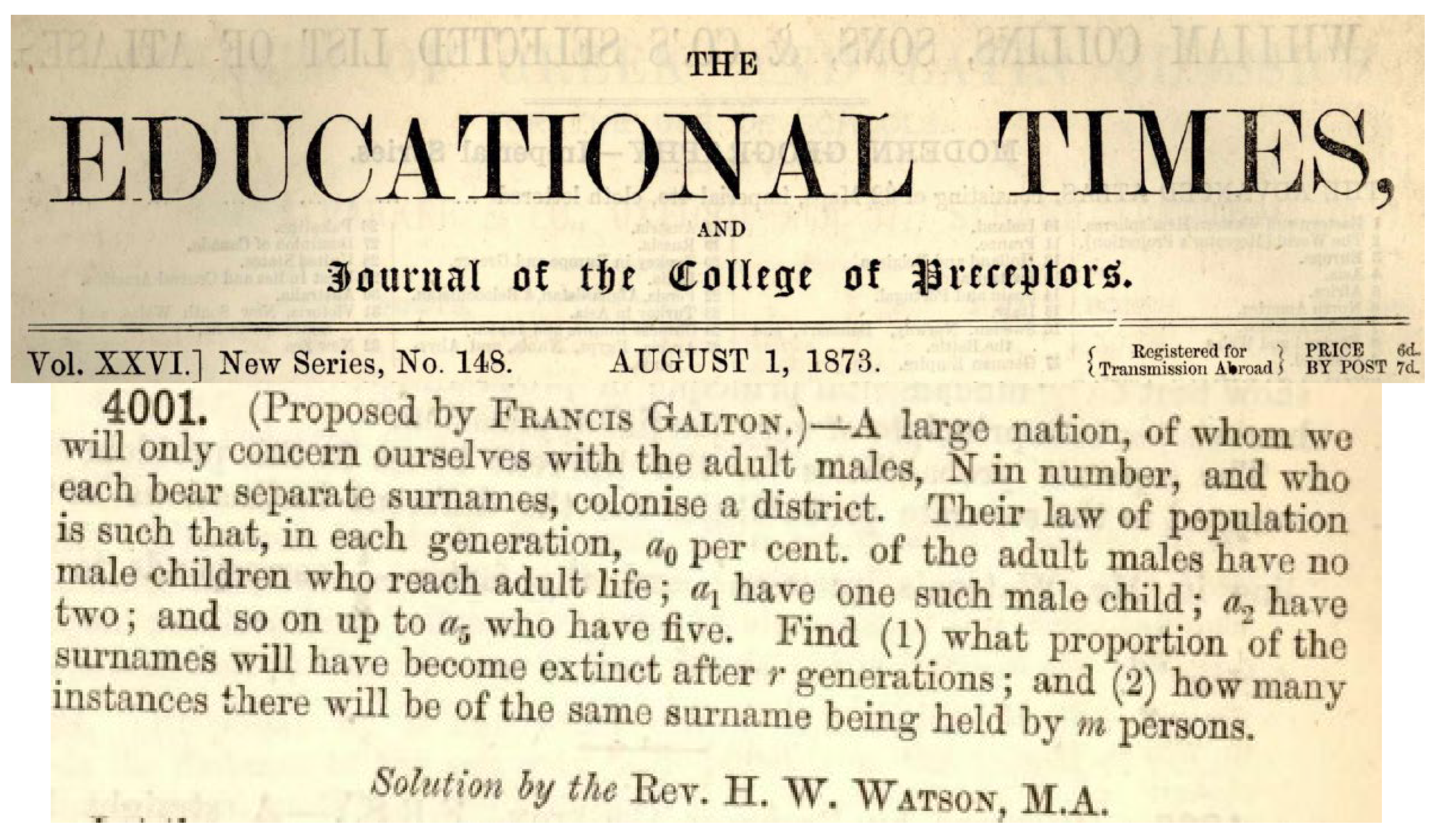
Figure 2.
Probability distribution of surnames with 0, 1, 2, … bearers after the first three generations, multiplied by 10000. Reproduction is specified by ak values, with .
Figure 2.
Probability distribution of surnames with 0, 1, 2, … bearers after the first three generations, multiplied by 10000. Reproduction is specified by ak values, with .
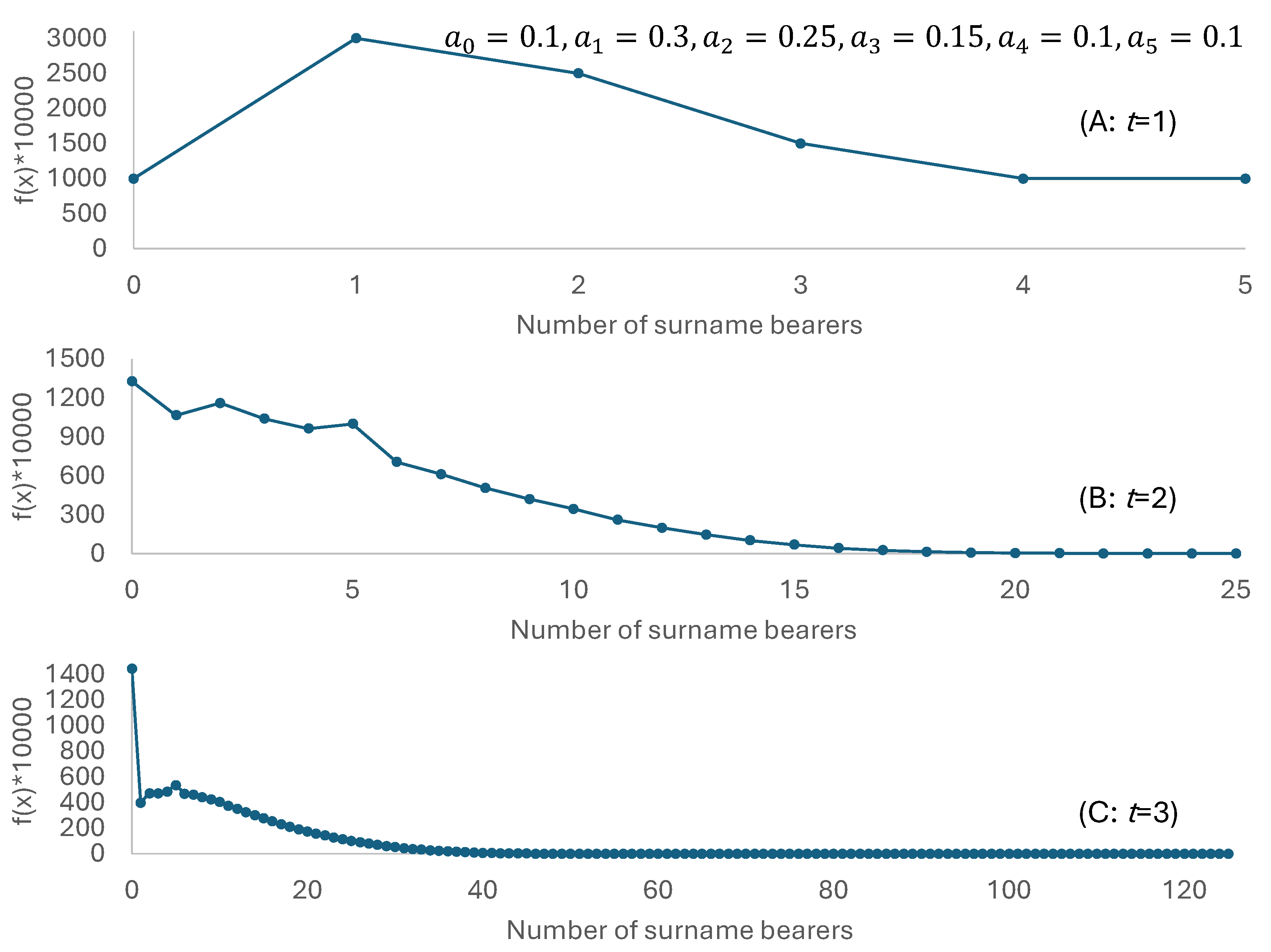

Table 1.
Numerical method for computing extinction time T and its variance.
| T | qt | qt−qt-1 | 1-qt | (2t+1)(1-qt) |
|---|---|---|---|---|
| 0 | 0 | 1 | 1 | |
| 1 | 0.5 | 0.5 | 0.5 | 1.5 |
| 2 | 0.7 | 0.2 | 0.3 | 1.5 |
| 3 | 0.808 | 0.108 | 0.192 | 1.344 |
| 4 | 0.872973 | 0.064973 | 0.127027 | 1.143245 |
| 5 | 0.914308 | 0.041335 | 0.085692 | 0.94261 |
| 6 | 0.941484 | 0.027176 | 0.058516 | 0.760704 |
| .. | … | … | … | … |
| 37 | 0.999999 | 3.75E-07 | 8.74E-07 | 6.56E-05 |
| 38 | 0.999999 | 2.62E-07 | 6.12E-07 | 4.71E-05 |
| 39 | 1 | 1.84E-07 | 4.28E-07 | 3.38E-05 |
| 40 | 1 | 1.28E-07 | 3E-07 | 2.43E-05 |
| .. | … | … | … | … |
| 92 | 1 | 1.22E-15 | 2.55E-15 | 4.72E-13 |
| 93 | 1 | 0 | 1.89E-15 | 3.53E-13 |
| 94 | 1 | 0 | 0 | 0 |
Table 2.
Relationship between λ and Q for . The calculation of W0 is explained in the text.
| W0(z) | Q | ||
|---|---|---|---|
| 1 | -0.36788 | -1 | 1 |
| 1.01 | -0.36786 | -0.99014 | 0.98034 |
| 1.1 | -0.36616 | -0.90630 | 0.82391 |
| 1.2 | -0.36143 | -0.82353 | 0.68627 |
| 1.3 | -0.35429 | -0.75013 | 0.57702 |
| 1.4 | -0.34524 | -0.68461 | 0.48901 |
| 1.5 | -0.33470 | -0.62581 | 0.41720 |
| 2 | -0.27067 | -0.40637 | 0.20319 |
| 3 | -0.14936 | -0.17856 | 0.05952 |
| 4 | -0.07326 | -0.07931 | 0.01983 |
| 5 | -0.03369 | -0.03489 | 0.00698 |
| 10 | -0.00045 | -0.00045 | 0.00004 |
Table 3.
The qt and qt − qt-1 for computing extinction time T and its variance Var(T) for .
| T | qt | qt − qt-1 |
|---|---|---|
| 0 | 0.0000000000 | |
| 1 | 0.3328710837 | 0.332871084 |
| 2 | 0.4800611401 | 0.147190056 |
| 3 | 0.5644334773 | 0.084372337 |
| 4 | 0.6193261945 | 0.054892717 |
| 5 | 0.6578744403 | 0.038548246 |
| 6 | 0.6863702213 | 0.028495781 |
| 7 | 0.7082254834 | 0.021855262 |
| 8 | 0.7254580952 | 0.017232612 |
| … | … | … |
| 999 | 0.8238658564 | 0 |
| 1000 | 0.8238658564 | 0 |
Table 4.
values for .
| T | ||
|---|---|---|
| 0 | 0 | |
| 1 | 0.1000000000 | 0.1000000000 |
| 2 | 0.1326610000 | 0.0326610000 |
| 3 | 0.1445833203 | 0.0119223203 |
| 4 | 0.1491044603 | 0.0045211400 |
| 5 | 0.1508434063 | 0.0017389461 |
| … | … | … |
| 23 | 0.1519416037 | 0.0000000001 |
| 24 | 0.1519416038 | 0.0000000000 |
| 25 | 0.1519416038 | 0.0000000000 |
Disclaimer/Publisher’s Note: The statements, opinions and data contained in all publications are solely those of the individual author(s) and contributor(s) and not of MDPI and/or the editor(s). MDPI and/or the editor(s) disclaim responsibility for any injury to people or property resulting from any ideas, methods, instructions or products referred to in the content. |
© 2025 by the authors. Licensee MDPI, Basel, Switzerland. This article is an open access article distributed under the terms and conditions of the Creative Commons Attribution (CC BY) license (http://creativecommons.org/licenses/by/4.0/).
Copyright: This open access article is published under a Creative Commons CC BY 4.0 license, which permit the free download, distribution, and reuse, provided that the author and preprint are cited in any reuse.


