
Submitted:
13 November 2025
Posted:
14 November 2025
You are already at the latest version
Abstract
Accurate binarization of phase-detection probe signals (gas vs. liquid) is necessary for the estimation of local void fraction, interfacial velocity, and bubble statistics in gas–liquid flows. Classical threshold based methods—single or double level— performs well on clean laboratory signals but degrades under realistic industrial conditions where noise, baseline drift, and clustered (slug-like) events challenge fixed rules. This work investigates whether deep learning (DL) models trained exclusively on synthetic data can deliver robust, generalizable binarization on real probe measurements. We (i) build a parametric generator of realistic time series from bubbly pulse templates, extended to clusters/slug patterns and perturbed with controlled noise, drift, and oscillatory baselines; (ii) train four lightweight DL architectures—one-dimensional U-Net (UNET-1D), Temporal Convolutional Network (TCN), a minimal one-dimensional Convolutional Neural Network (CNN-1D), and a Bidirectional Long-Short Memory network (BiLSTM)—only on synthetic signals; and (iii) evaluate them against classical threshold methods using event-level and sample-level metrics. On synthetic signal evaluation, UNET-1D and TCN achieve near-perfect event detection and sub-millisecond onset errors. On real bubbly and slug flow sensor data, classical threshold based methods remain highly competitive on clean sensor signals, while DL models retain advantages under non-stationary baselines and clustered events, yielding accurate void and timing with no hand-tuned assumptions. Results support DL as a practical, data-driven complement to fixed algorithms, particularly in noisy or drift-dominated measuring conditions.
Keywords:
intrusive sensors
; deep learning
; flow parameters
; phase identification
; signal processing
; two-phase flow
1. Introduction
Gas–liquid two-phase flows are central to nuclear thermal–hydraulics and many allied engineering applications, including reactor coolant systems, safety-relevant components, heat exchangers, chemical reactors, and multiphase transport lines. Accurate local measurements of interfacial quantities—void fraction (), bubble chord lengths () and interfacial velocities (), interfacial area concentration (IAC), and interface frequency—are essential for mechanistic modeling (e.g., two-fluid models and closure relations), code validation, and system design and safety analysis. In test facilities where optical access is limited or non-intrusive modalities are impractical, intrusive phase-detection probes have become the workhorse for obtaining time-resolved, local information about the phase present at the probe tip. Single- and multi-tip optical fiber probes, as well as conductance/resistive probes, have been widely used to infer local void fraction, interface velocities (often via multi-sensor time-of-flight), and IAC with appropriate signal interpretation [1,2,3,4].
Despite their widespread adoption, the accuracy of intrusive probes ultimately hinges on how raw voltage (or optical) signals are interpreted. The canonical workflow converts a continuous, noisy waveform — generated as the interface pierces and leaves the probe tip—into a binary (two-state) gas–liquid series, from which event durations and inter-sensor delays yield the target local parameters. In relatively simple bubbly flows with well-separated bubbles, simple amplitude thresholding method can be adequate. However, as flow regimes become more complex (e.g., bubble clustering, transitional bubbly-to-slug, higher void fractions), fixed-threshold methods deteriorate: baseline drift, probe/electronics response, local deformation of the interface during piercing, and multi-peak bubble signature superposition produce ambiguous leading/trailing edges, peak broadening, and sub-threshold events that classical schemes tend to miss [2,3,5]. These issues have been documented for optical and conductance probes alike, motivating sustained investigations into probe response, uncertainty quantification, and improved signal treatment strategies [4,6].
Two complementary lines of progress can be traced in the literature. The first improves the measurement physics and processing of multi-sensor probes. Four-sensor arrangements enable 3D interface velocity vectors and orientation, and provide access to IAC via local counting with geometric pairing. Correction and evaluation studies—particularly for bubbly flows—quantify biases stemming from finite tip spacing, bubble shape distortion, and velocity fluctuations, and propose numerical corrections and pairing logic to reduce systematic errors. Comparative works benchmark four-sensor against double-sensor probes across regimes, underscoring that even with sophisticated geometries, the limiting factor often remains robust event detection and pairing in noisy signals [6,7,8,9].
The second line targets signal processing of single-sensor signals to determine bubble entry/exit times reliably. Beyond single-threshold methods (mean/median or fixed fractions of the signal span), dual/multiple thresholds, slope-based triggers, and adaptive schemes that track local extrema and evolving baselines have been explored. For industrial-scale bubbly flows, robust algorithms have been proposed to mitigate noise sensitivity and to improve segmentation within clustered events; yet these approaches still depend on user-defined parameters (e.g., thresholds, minimal distance between extrema, smoothing windows), and performance can degrade under strong baseline drift or when small-amplitude events are embedded within clusters [5]. The consequences are well known: underestimation of void fraction and interface counts, biased interfacial velocities, and inconsistent IAC precisely in the regimes of greatest practical interest [10,11,12].
From a nuclear-thermal–hydraulics perspective, accurate local interfacial measurements feed directly into closure correlations and interfacial transport equations. Archetypal developments of local IAC measurement and modeling within the two-fluid framework highlight both the utility of intrusive data and the sensitivity of inferred quantities to detection uncertainty: any method that consistently shifts entry/exit times or misses multi-sensor events will propagate errors into IAC and velocity statistics, thereby obscuring physical trends and compromising model validation [13,14]. This tight coupling between signal interpretation and two-phase modeling amplifies the value of processing techniques that generalize across regimes and sensors.
In parallel, learning-based methods have transformed time-series analysis in many engineering fields. Recurrent neural networks (RNNs) and gated variants (e.g., LSTM and bidirectional LSTM, Bi-LSTM) capture long-range temporal dependencies in non-stationary signals, while hybrid pipelines blend light, domain-motivated preprocessing (e.g., signal derivatives and signal envelopes) with trainable models to achieve robustness under noise and drift. In spectroscopy and other high signal-to-noise domains, learning-based baselining has proven effective where hard-coded or rule-based corrections struggle [15]. These trends suggest that the phase-detection problem—a one-dimensional segmentation task on a waveform corrupted by stochastic and systematic artifacts—could benefit from deep sequence models that learn event morphology directly from data rather than relying on brittle thresholds.
Two factors, however, have historically impeded direct adoption of deep learning for probe signal interpretation. First, curating sufficiently large, expert-labeled datasets is labor-intensive: precise marking of entry/exit moments for thousands of bubble encounters is time-consuming even for trained analysts. Second, data diversity—across probe types, tip geometries, electronics, sampling rates, and flow regimes—complicates model generalization. In this scenario, synthetic data offer a principled remedy: if one can procedurally generate realistic bubble-signature waveforms with controllable morphology, signal-to-noise ratios, baseline drift, and clustering statistics—and if one can combine them with a curated test dataset of real, manually labeled segments—the resulting dataset can (i) expand coverage of edge cases, (ii) embed physical priors about waveform shape, and (iii) provide exact ground-truth (GT) for training while keeping labeling tractable and only for testing. Earlier skill-based approaches (e.g., using genetic algorithms informed by expert annotations) demonstrated that encoding human expertise into automated discriminators can markedly improve classification robustness [16,17].
Within this context, the present work test the hypothesis that compact DL sequence models, trained exclusively on synthetic waveforms, can recover the per-sample binarization and onset/offset timing required to process phase-detection probe signals in gas–liquid flows, with performance that transfers to real measurements. This question is not merely academic: in nuclear thermal-hydraulics, local two-phase descriptors—void fraction, interfacial velocity, and interfacial area concentration (IAC)— are of the utmost importance for the development and validation of subchannel and system-scale closures, as well as the interpretation of integral-effects tests. Conductivity/optical phase-detection probes remain among the few instruments that can be deployed in opaque or geometrically constrained test sections typical of nuclear loops, but their signals are notoriously sensitive to noise, drift, and bubble–tip interaction effects, which complicates threshold-based segmentation and event pairing used in multi-sensor probes [1,2,4,5].
A central obstacle for a reliable method development is the sensor signal GT. In nuclear-relevant facilities, optical access is limited and interface contacts cannot be timestamped reliably at scale. High-speed imaging is feasible only in selected geometries and still struggles to mark the exact liquid→gas () and gas→liquid () instants because of interface deformation, meniscus dynamics, and tip “crawling” [4]. As a result, most validation is forced to rely on aggregate checks—e.g., comparing time-averaged void fraction against pressure-drop or superficial-velocity estimates. Such integrals are necessary but insufficient: they conflate missed bubbles with overfilled plateaus and provide little insight into onset timing, which directly enters interfacial-velocity and IAC estimates [6,14]. Two very different segmentations can yield similar mean void, masking serious biases in bubble dimensions (via bubble chord length estimation) or interfaces timing. Progress therefore demands bubble-resolved ground truth to evaluate algorithms at the event level, in timing, and in coverage/overfill—not just in global void.
To meet this need, we construct a synthetic signal framework explicitly inspired by measured traces: logistic rises are fitted to hand-labeled bubbly pulses and then composed into isolated events, clusters, and slug-like chords. We inject controlled nuisances—white noise, slow drift, and sinusoidal baseline oscillations—so that the training distribution spans the degradations that undermine classical thresholding in practice [5]. Crucially, synthetic generation provides exact, per-sample labels (including unambiguous ), enabling large-scale supervision that is virtually unattainable in real campaigns [1,2,18].
On top of this generator we train a compact, complementary set of models—UNET-1D, TCN, CNN-1D, and BiLSTM—under a unified pipeline (per-record z-score normalization, class weighting, softmax head). Each network emits a posterior that is binarized by a single threshold chosen on synthetic validation to maximize event-level and then frozen for real-signal tests. As rule-based comparators, we include (i) an enhanced single-threshold method (median-referenced level plus local-extrema parsing to stabilize ) and (ii) a double-threshold/hysteresis variant that segments clustered peaks using slope intersections [5]. We then evaluate all methods on short real traces representative of bubbly (isolated pulses) and slug (clustered, ambiguous baseline) regimes, and on stress cases built by superimposing a sinusoidal baseline onto the real signals—conditions germane to nuclear loops, where electromagnetic interference, temperature-dependent conductivity, and flow-regime transitions are common.
The ensuing analysis is organized around a minimal, application-driven set of metrics—event-level , onset MAE/P95, coverage/overfill, and void-fraction bias—consistent with the local-parameter definitions standard in two-phase metrology [6,14]. Anticipating the results, compact DL models trained only on synthetic data preserve timing fidelity and curb failure modes precisely where thresholding degrades (noise, drift, clustering), supporting their use as a practical, software-only alternative for interpreting intrusive probes in nuclear thermal-hydraulic experiments.
Hereafter, the paper is organized as follows. Section 2 formalizes the local two-phase descriptors and timing conventions (such as void fraction, chord/onset–offset definitions), introduces the classical signal processing methods (enhanced single-threshold and double-threshold/hysteresis), details the synthetic signal generator and perturbation algorithm, and describes the DL architectures, dataset preparation, and evaluation protocol along the evaluation metrics. Section 3 presents a three-stage assessment: (i) a clean synthetic benchmark spanning isolated pulses, clusters, and slug-like chords; (ii) two real hold-out traces representative of bubbly and slug regimes; and (iii) stress tests obtained by superimposing a sinusoidal baseline on those real signals. Comparisons emphasize event-level detection (F1evt), onset timing (MAE/P95), coverage/overfill, and void bias, with qualitative overlays for interpretability. Section 4 summarizes the general conclusions of presented study. The companion code used for data generation, model training, trained models, datasets used and evaluation is openly available at DOI 10.5281/zenodo.17551695 for full reproducibility.
2. Materials and Methods
This section formalizes the quantities and signal morphologies relevant to phase-detection probes and outlines the processing pipelines evaluated. We begin by defining the two-phase descriptors used throughout—void fraction , chord–based quantities, and their linkage to event onsets/offsets—and by illustrating typical pulse patterns in bubbly and slug regimes. We then summarize the classical baselines adopted as comparators (single-threshold with a median reference and a double-threshold hysteresis scheme, plus a simple cluster-aware variant), describe the synthetic signal generator that assembles logistic-rise bubbles into isolated events, clusters, and slug-like segments under controlled noise/drift/oscillation while providing per-sample ground truth, and present the deep models (UNET-1D, TCN, CNN-1D, BiLSTM) with the dataset preparation steps (per-record z-score normalization, fixed-length windowing, class weighting, unified classification head). Finally, we outline the evaluation protocol at a high level—training on synthetic data and transferring a per-model decision threshold selected on synthetic validation to real traces—while deferring the formal metric definitions (event-level , onset timing MAE/P95, coverage/overfill, and void bias) and the stress tests to the beginning of Section 3.
2.1. Local-Flow Parameters
Processing intrusive probe signals reduces to identifying, within the raw voltage trace, the time intervals that correspond to gas passages (bubble chords). Operationally, this requires locating for each bubble signature the probe entry time (liquid→gas) and exit time (gas→liquid). Once these moments are known, the principal local parameters—void fraction, interfacial (axial) velocity with two axially separated sensors, bubble frequency, chord statistics, and interfacial area concentration (IAC)—follow directly.
Let T be the total acquisition time. The time-based local void fraction is
where is the gas-occupancy duration (or time chord) of the i-th detected bubble at the probe location. The event (bubble) frequency is , with N the number of detected chords or front/rear interfaces.
When two sensors are available, separated axially by a known distance along the mean flow, an average interfacial (axial) velocity can be estimated from leading-interface time-of-flight:
where is the measured delay between the leading interfaces detected by the upstream and downstream sensors for bubble i, and counts effectively paired events or interfaces.
For each chord, we define the spatial chord length as:
where is the interface speed component along the probe piercing direction (unit normal ). In a two-sensor axial arrangement, can be approximated by when alignment with the mean flow is adequate; otherwise, can be interpreted as the path length traversed by the interface through the sensitive volume. Chord-length distributions summarize local bubble-scale geometry and, together with , and , provide a compact description of regime changes (isolated bubbly versus clustered/slug conditions).
Following [14], the local time-averaged interfacial area concentration (IAC) can be written as:
Equations 1–4 show that accurate , velocity, chord-length statistics, and IAC all hinge on consistent determination of and for every bubble signature and, when applicable, reliable pairing of interfaces across sensors to obtain .
Figure 1 serves to depict previous relevant signal event-points but also serves to describe several practical aspects of signal interpretation which are common to most processing algorithms:
- Peaks in the probe voltage correspond to interactions of the probe tip with the gas phase (bubbles).
- The determination of (first liquid→gas transition) is non-trivial even for trained operators. Uncertainty zones (dashed boxes in Figure 1) vary from bubble to bubble due to shape, the radial piercing location of the bubble relative to the tip [4], local curvature () and surface tension effects, etc. Similar ambiguity arises for (gas→liquid).
- Choosing an adequate discrimination baseline is critical. Using the liquid-level voltage as baseline is sensitive to noise; using a threshold displaced from (e.g., ) mitigates noise but may shorten the detected gas plateau and hence underestimate .
- Slope-based schemes with two or more thresholds (e.g., and ) infer / from pairs of signal crossings points at and and (A-A’ and B-B’). However, even for the same bubble, the rise/fall shapes may differ between the front and rear sensors, introducing variability in the derived parameters.
These considerations motivate robust rules for and extraction and, when available, careful pairing of interfaces between sensors to compute in Equation (2).
To assess out-of-domain transfer from purely synthetic training to real measurements, we evaluate the processing methods on short (∼5 s) sensor signals acquired in a vertical, upward air–water loop. The facility consists of a 5 m vertical pipe (inner diameter mm) able to sustain regimes from disperse bubbly to annular. Water temperature is regulated by a heat exchanger in the reservoir; all data used here were recorded at 20 °C. Downstream of the two-phase injection chamber (conical plenum with four liquid injectors and four porous air inlets), instrumentation ports at Z(height)/D = 22, 61 and 99 provide flush access for four-sensor conductivity probes mounted on a motorized traverse for precise radial positioning. Signals were digitized with a National Instruments NI-PCX-6333 DAQ (aggregate capacity ∼1.2 MHz); in this study we operated at kHz per channel across 12 channels. Full facility and probe details are provided in [19].
For evaluation, we selected representative segments from two canonical regimes: (i) bubbly flow (Figure 2, characterized by well-separated pulses and sparse clustering; and (ii) slug flow Figure 3, featuring clustered transients, Taylor-bubble plateaus followed by trains of small bubbles, and therefore promoting an ambiguous baseline voltage compared to the bubbly flow regime. GT for these hold-out traces is the per-sample binary mask obtained by expert manual labeling of event onsets/offsets, consistent with the onset-matching tolerance used in Section 2.4.
2.2. Signal Processing: Single and Double-Threshold Methods
Single-thresholding is the simplest and historically most used approach for intrusive probes [2]. A single reference voltage discriminates gas from liquid on a per–sample basis: samples above are labeled as gas, those below as liquid. A convenient parametrization is
where and are the minimum and maximum sensor voltage output of the analysed signal segment. In practice, two robust special cases are widely used: setting to the global mean (Mean) or to the global median (Median) of the signal, which reduces sensitivity to outliers.
To improve robustness without leaving the single–threshold paradigm, we adopt two lightweight refinements:
- Segment-wise refinement. After the raw binarization, each continuous gas-labeled segment is processed independently to determine its salient timestamps. Within a segment, we assign the exit time at a local maximum and the entry time at the closest preceding local minimum. Local extrema are obtained with a modified peakdet routine [20], using a prominence of 10% of the signal span and enforcing a minimum separation consistent with sampling rate and expected bubble chord lengths. This reduces fragmentation by high-frequency noise and yields consistent onset/offset markers in broad or low-contrast peaks [19].
- Local context for and determination in cluster events. When several small fluctuations occur within one gas-labeled segment (clusters), only the dominant extremum pair (by prominence) is used for , preventing spurious multiplication of events and the derived bias in void fraction.
These add-ons keep the method simple and fast while mitigating common failure modes of plain thresholding method. A residual limitation persists in clustered regimes: if individual sub-bubbles within a cluster do not rise above or the waveform does not return close to baseline between sub-events, single–threshold binarization tends to merge multiple interfaces into one, biasing both and interface counts.
To address cluster segmentation and reduce sensitivity to slow drift, double–threshold methods introduce two levels following [5]: a lower threshold near the liquid level and a higher threshold within the typical peak range. The procedure is:
- Any crossing of starts a candidate gas event. If the transient never exceeds , the event limits are the crossings (/).
- If the transient exceeds , peaks inside a cluster are delineated by intersecting rising and falling slopes of adjacent transients; consecutive / are assigned at those intersection points (shifted by one sample to avoid degeneracy).
- As in the single–threshold refinement, local extrema (via the same peakdet constraints) are used to fine-tune within each candidate segment.
These variants improve intra–cluster segmentation and are less sensitive to slow baseline wander than using the liquid level directly. Nevertheless, they still rely on user–chosen parameters (two thresholds, minimum distances) that may require retuning when electronics, noise characteristics, or flow regimes change [4,5].
As stated previously, accurate computation of the flow descriptors hinges on consistent identification of / for every bubble signature and, when applicable, reliable pairing across sensors. Threshold–based methods are attractive for their transparency and computational frugality, and they perform satisfactorily in bubbly conditions with well-separated peaks. However, performance degrades with (i) elevated noise, (ii) baseline drift, and (iii) clustered or slug–like patterns where individual sub–events may not surpass fixed levels or return to baseline between pulses. In such regimes, enhanced single–threshold methods tend to undercount interfaces and bias , while double–threshold slope–based schemes alleviate but do not eliminate these issues [4,5]. These limitations motivate the data–driven approach evaluated in this work, where compact deep models learn discriminative transient shapes and timing from synthetic but physically informed exemplars, reducing the dependence on hand–tuned thresholds and heuristic post–processing.
2.3. Synthetic Signal Generation
To train and benchmark the segmentation models under full GT control, we synthesized multiple long one–dimensional sensor traces that emulate the voltage response of a local phase–detection probe as bubbles traverse the sensing region. For each discrete sample n (sampling rate ), the generator outputs a voltage trace and a binary label , with whenever gas is in contact with the probe. The procedure reproduces the canonical pulse morphologies observed in bubbly and slug regimes while allowing controlled perturbations of the baseline (broadband noise and slow oscillations). The methodology used for this purpose is as follows. We first extract representative rising edges from hand–labeled, isolated bubble events in real traces and fit them with a logistic front, as depicted in Figure 4. This choice is pragmatic: the logistic simultaneously captures the steep onset and its gradual saturation, and it can be scaled to different chords (durations) and amplitudes without introducing discontinuities. We summarize this family with a compact logistic front whose steepness is controlled by a single parameter b:
where A is the pulse amplitude, is the index of the half-height crossing, and sets the interface sharpness perceived by the probe.
The pulse chord (duration) is specified by . To obtain a smooth return to baseline we append a short polynomial decay (tail),
with . In synthesis, are randomized within empirical ranges inferred from the pooled slopes, thereby reproducing the spread of onset sharpness and durations seen in real traces.
We assemble three pulse families to span the range of flow regimes:
- Isolated bubbles (bubbly). A single pulse with chord drawn uniformly (e.g., 100–400 samples), amplitude A randomized within a prescribed range, and tail as in Equation 7.
- Slugs. A logistic rise to a high level followed by a plateau and a tapered tail. The plateau length is set as a multiple of the rise (e.g., a factor in 10–20), producing sustained gas occupancy that must remain “on” without flicker.
- Clusters. A sequence of bubble pulses placed with partial overlap so the signal does not return to baseline between arrivals. We draw an overlap fraction and start each new member within of the previous pulse extent. Where pulses coincide, the sample-wise maximum is taken to emulate probe saturation. The cluster is labeled as a single continuous gas interval: from the first onset to the last offset for each bubble trace.
An example of two different regimes synthetic signal are depicted in Figure 5
Events are positioned at random, non-overlapping locations on a long timeline by maintaining an occupancy mask. Generation proceeds until a target mean void fraction is reached.
The final voltage trace is obtained as the superposition of a nominal baseline, broadband noise, low-frequency oscillation, and the synthesized events:
Here models uniform white noise around the nominal 1 V baseline; the sinusoid with amplitude and frequency introduces slow baseline wander representative of thermal/electromagnetic drift; and aggregates all placed pulses (isolated, slug, clusters). These two knobs-—broadband noise and low–frequency oscillation—-span the dominant degradation modes observed in practice, while preserving an exact binary ground truth by construction.
All random draws (event types, durations, overlaps, amplitudes, positions, and noise parameters) are governed by a stored in a random state, ensuring exact reproducibility. Along with and , the generator saves the full configuration (sampling rate, target , ranges, and seeds). In practice, the setup yields diverse long sequences mixing isolated spikes, long plateaus, and densely packed clusters across a wide range of perturbation levels—precisely the coverage needed to train robust models and to stress–test classical thresholding under controlled, known–truth conditions. The MATLAB implementation and presets used in this work are available in the companion repository provided in the Data Availability Statement.
2.4. DL-Based Signal Processing and Evaluation Metrics
Deep learning (DL) has not, to the best of our knowledge, been applied directly to determine bubble entry/exit times from intrusive probe voltage signals. A conceptually related line of work used genetic algorithms informed by human expertise to optimize phase discrimination in noisy probe records [16,17]. In another domain that faces analogous challenges—accurate peak detection over drifting, noisy baselines—adversarial neural networks have been proposed for baseline correction in spectroscopy [15]. These precedents share the same core difficulty encountered in two-phase probe processing: reliable identification of transient features (peaks, onsets, shoulders) in signals affected by high-frequency noise and low-frequency drift.
As stated previously in Section 1, a principal obstacle for applying DL to phase detection is the preparation of suitable training data. Modern neural networks benefit from large, diverse, and accurately labeled datasets. In the context of intrusive probes, creating such a dataset requires the manual annotation of bubble moments (entry and exit ) in raw signals, a task that is time-consuming, prone to subjective variability, and often limited by data availability. Although extensive post-processed databases exist in the literature, raw time series with ground-truth labels are scarce, and the diversity of sensor designs and operating conditions further complicates generalization.
To address these constraints, we adopt a training strategy based only on controlled but reallistically generated synthetic sensor signals. The intent is twofold. First, to exploit synthetic signals as a scalable source of exactly labeled examples (with known and ), thereby enlarging the training set and covering edge cases (weak peaks, overlapping events, clusters) that may be underrepresented in real data. Second, to extend realism by incorporating real-like signal perturbations encountered in industrial conditions so that the model learns those characteristic distortions to extend its inference performance.
With this goal, this study adopts a compact yet complementary set of sequence-to-sequence classifiers to convert raw probe voltages into per-sample gas/liquid labels: a one-dimensional U-Net (UNET-1D), a temporal convolutional network (TCN), a minimal convolutional baseline (CNN-1D), and a bidirectional long short-term memory network (Bi-LSTM). The selection spans distinct inductive biases—multi-scale encoder–decoder, dilated temporal convolutions, local convolutional morphology, and recurrent temporal context—while keeping the benchmark lightweight and reproducible. The complete implementation in MATLAB (exact layer graphs, training options, synthetic-signal generator, and evaluation scripts for normalization, threshold selection, and metric computation) are archived in a public repository and can be cited and accessed via the DOI 10.5281/zenodo.17551695 to enable faithful replication and reuse without inflating the manuscript with implementation details. Considered DL model architectures are briefly introduced as follows:
- UNET-1D: The 1-D U-Net comprises an encoder–decoder with three down/up stages and lateral skip connections. Downsampling increases the temporal receptive field, allowing the model to capture contextual trends (e.g., pre-onset fluctuations or baseline drift), while skip connections preserve high-frequency detail for precise onset timing. In bubble detection, pulses are brief (sub-millisecond onsets at 40 kHz) yet their detectability benefits from broader context; UNET-1D therefore operationalizes a multi-scale, localization-preserving paradigm well matched to event detection with sharp onsets. Our use follows the U-Net paradigm introduced in biomedical segmentation [21] and subsequent 1D adaptations for physiological waveforms [22].
- TCN: The TCN employs stacks of dilated 1-D convolutions with residual connections. Dilation expands the receptive field exponentially without pooling, preserving sequence length and enabling efficient, fully convolutional inference. Residual shortcuts stabilize optimization in deeper temporal stacks. TCNs are well suited to long-range dependencies, which is pertinent to slug regimes characterized by clustered events and ambiguous baselines. Relative to recurrent models, TCNs offer favorable parallelism and latency on GPUs or embedded accelerators. We ground our choice in the TCN sequence-modeling literature [23,24] and the application of TCNs to time-series classification and hydrologic forecasting [25,26].
- CNN-1D: We include a carefully tuned two-layer 1-D CNN (with batch normalization and ReLU) followed by a compact fully connected head as a strong local baseline. This architecture primarily exploits short-range morphology (peak shape and its immediate neighborhood) at low computational cost. It serves to quantify the incremental benefit of multi-scale (UNET-1D) and long-context (TCN) mechanisms over a well-engineered local detector, and provide a reference when datasets or hardware are constrained.
- Bi-LSTM: A single bidirectional LSTM layer with a small Multi-Layer Perceptron (MLP) head provides recurrent temporal context. The bidirectional state can smooth short-term fluctuations and encode dependencies that are not strictly convolutional, improving robustness to baseline drift and irregular pulse spacing. Although recurrent models are less parallel than TCNs, Bi-LSTM remains a recognized baseline for noisy temporal classification and enriches the diversity of inductive biases in our set. Bi-LSTMs remain a recognized baseline for noisy temporal classification, with classical foundations in bidirectional RNNs [27] and strong empirical performance for physiological signal segmentation [28,29].
We intentionally exclude heavier families (e.g., Transformer encoders, attention-augmented hybrids, or ensembles) to avoid conflating model capacity with post-hoc tuning and to keep training/inference budgets modest. Likewise, we do not stack conditional random fields or handcrafted rules on top of network scores. The comparison is purposely intended: each network outputs per-sample posteriors and is evaluated under the same decision rule described in the next section.
The networks are trained to classify each time sample as liquid or gas. We use mini-batch optimization with Adam (learning rate ) and monitor standard validation metrics to avoid overfitting. All models are trained as per-sample classifiers with a softmax cross-entropy head. Inputs are single-channel sequences sampled at kHz; outputs are posteriors . At evaluation time, a single scalar threshold binarizes the posterior,
To prevent ad-hoc tuning and isolate model capacity, we employ a frozen-threshold protocol: for each model, we select a threshold on the synthetic dataset by grid search to maximize event-level F1evt), and we then keep unchanged for the real signal evaluations. No smoothing, hysteresis, or event fusion is applied to predictions. This design is aimed to remove confounders, improve reproducibility, and to reveal each architecture’s precision–recall behavior when the test distribution departs from training (movig from synthetic signals to real sensor signals inferences). In operational deployments, where spurious triggers, o or false detections, are costly, can be re-tuned per site or regime without modifying model weights; however, such adjustments are outside the scope of the present comparison.
The goal is therefore twofold: (i) to recover from a single phase–detection probe a per–sample binary sequence that marks gas presence, and (ii) to preserve the timing of individual bubble traces, the onset/offset instants that define the interfaces. We therefore report a compact set of complementary metrics: (a) event–level detection quality, (b) onset–timing accuracy, (c) temporal coverage/overfill, and (d) void fraction bias. All quantities are computed in discrete time at sampling rate . To quantitatively assess the performance of the segmentation algorithms, we employ a set of complementary metrics that evaluate detection quality, onset timing accuracy, temporal coverage, and overall gas occupancy estimation. The methodology is designed to reflect both event-wise correctness and signal-level fidelity.
Let the ground–truth event set be and the predicted set , where denote integer sample indices. We perform a one–to–one, greedy pairing by onset proximity: a prediction k is a true positive (TP) if there exists an unused i with ; otherwise it is a false positive (FP). Ground–truth onsets left unmatched are false negatives (FN). Here is a fixed tolerance in samples (set a priori; in our experiments, with ms).
From this pairing, we compute:
Here, GDR refers to GT detection rate (analogous to recall), and is the harmonic mean of precision and GDR at the event level. We also report the raw count of false positives, which is particularly informative in diagnosing over-segmentation or spurious detections due to noise.
In order to evaluate the onset–timing accuracy for each matched pair we compute the absolute onset error in seconds,
We summarize timing quality with the mean absolute error and the 95th percentile . Small values indicate low jitter in interface timing, a prerequisite for accurate and determination using multi-sensor probes, as described in Section 2.1.
Let and be the ground–truth and predicted binary masks, . Over the record duration , we compute the fractions for the temporal coverage (COV) and overfill (OVL) as:
COV measures how much of the true gas occupancy is retrieved, meanwhile OVL penalizes predicted gas outside the true support (useful to expose leakages due to drift or baseline oscillations).
We track the gas duty cycle or on each record,
and report the bias . This physically interpretable aggregate complements event–level measures and reveals systematic under/over–estimation of gas occupancy.
The chosen metrics deliberately balances what is detected (event counts via and FP), when it is detected (MAE/P95 of onsets), and how much is detected (coverage/overfill and void bias). Event–level avoids misleadingly high per–sample accuracy under class imbalance; onset MAE/P95 connects directly to interfacial velocity errors or interface timing; COV/OVL provides an occupancy–centric view useful for diagnose drift and segmentation failures; and offers a compact check against physically meaningful averages.
3. Results and Discussion
This section assesses the four deep models (UNET-1D, TCN, CNN-1D, Bi-LSTM) and two threshold-based baselines, single-threshold with enhanced cluster aware modifications (1-TH) and two-thresold or slope method based on [5] (2-TH) under progressively demanding conditions. Metrics and the onset-matching protocol were defined previously in Section 2.4; here we report event-level detection (), onset timing (MAEonset, P95onset), temporal COV and OVL, and void estimation ( against GT void ). We also report the GT number of labeled incoming bubble interfaces () to be compared to the number of interfaces inferred by the different methods ()
We organize the analysis in three blocks. First, we present a representative synthetic case generated by the proposed pipeline, with wide variability in pulse shapes and clusters but no additive noise or baseline oscillation (Table 1). This establishes an optimistic ceiling and quantifies how much a minimal DL model (with CNN-1D setting the baseline) can achieve when evaluated with clean signals similar to training dataset. Second, we move to real sensor measurements at two regimes: a bubbly case with isolated peaks and limited clustering, and a slug case with Taylor bubbles followed by dense trains of small bubbles (Table 2 and Table 3). These tests probe robustness to realistic buble signature variability, amplitude dispersion, and imperfect baselines but obtained in controlled scenario (laboratory scale). Third, we apply an oscillatory baseline perturbation to both real sensor signals with severe low-frequency oscillation, emulating a complex industrial-like scale measurement. Latest comparison serves to challenge all methods in the most challenging scenario. In brief preview, the synthetic case shows all deep models near ceiling, with CNN-1D already very strong; in real bubbly/slug, UNET-1D and TCN maintain the best balance of , timing, and void fidelity, whereas 1-TH and 2-TH lag increasingly as clustering and baseline ambiguity grow; under oscillatory stress, the gap widens further, with learned models retaining high recall and low overfill while fixed thresholds trade detection precision for bias in the estimation. Detailed values and per-case observations follow.
3.1. Synthetic Signals Evaluation
We first establish an upper bound on achievable performance by evaluating all methods on a clean synthetic trace, depicted in Figure 7 that spans wide morphological variability (isolated pulses, clusters, and slug-like plateaus) but contains no additive noise or baseline oscillation.
Figure 6.
Synthetic signal and its GT used to evaluate proposed models.
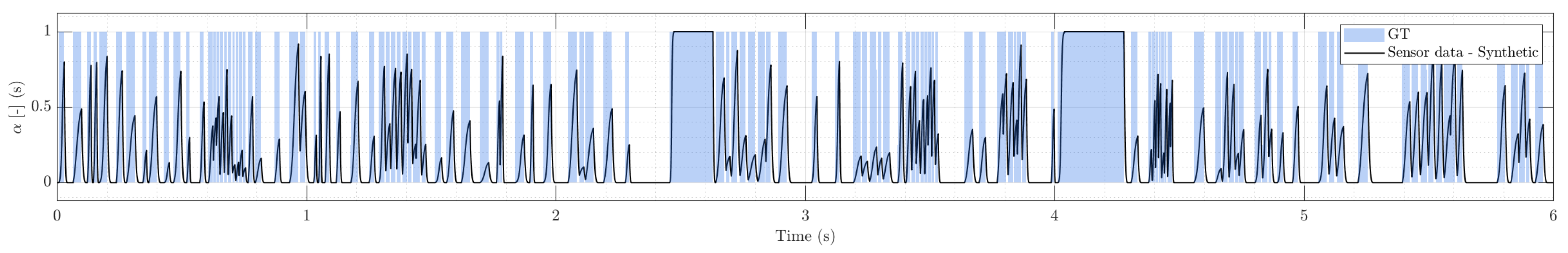
Figure 7.
Detail of synthetic evaluation dataset segmentation: Threshold-based methods (top) and DL models inferences (bottom).
Figure 7.
Detail of synthetic evaluation dataset segmentation: Threshold-based methods (top) and DL models inferences (bottom).
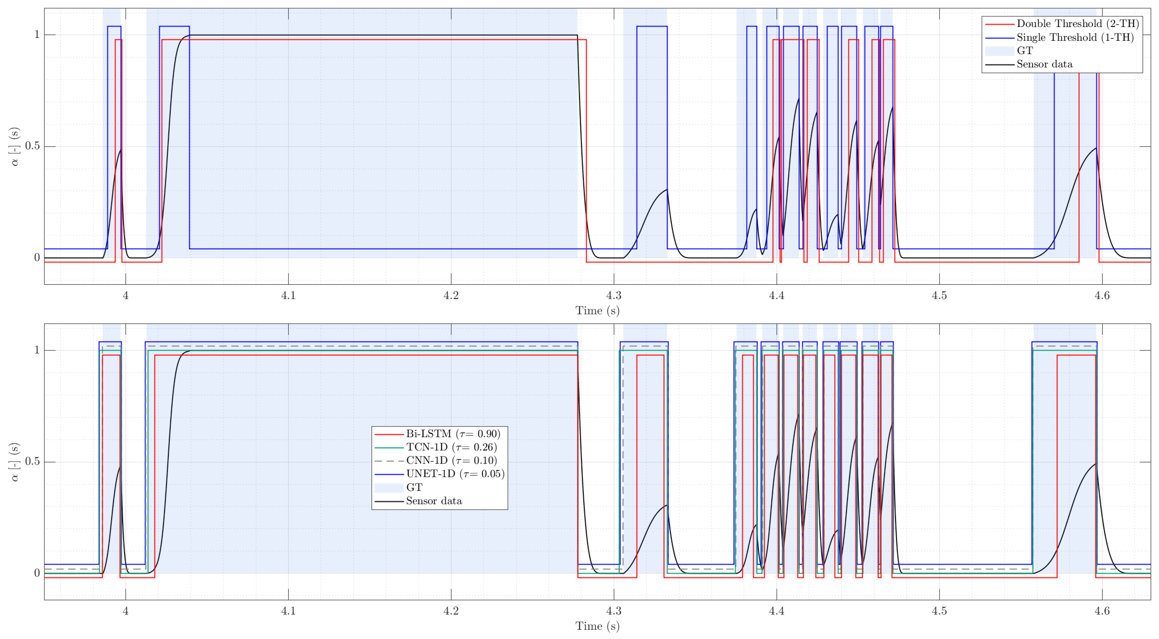
As shown in Table 1, the three deep architectures with convolutional architectures approach ceiling performance at the event level, while recurrent architecture (Bi-LSTM) remains close but slightly more conservative in coverage and timing. In contrast, 1-TH is competitive in detection but exhibits substantially larger timing errors and a marked negative bias in the recovered ; the 2-TH underperforms in this setting due to its conservative splitting rules.
Concretely, TCN attains perfect event detection () with low onset error (MAE ≈ 1.15 ms, P95 ≈ 3.52 ms) and near-neutral void bias (). UNET-1D and the CNN-1D baseline are essentially tied in event detection () with excellent timing; notably, CNN-1D achieves the lowest MAE (0.22 ms) and a negligible void error (). Bi-LSTM also reaches near-ceiling event scores () but, consistent with bidirectional temporal smoothing, shows a modest reduction in coverage () and a slight negative void bias ().
Among classical threshold-based methods, 1-TH achieves a high () but incurs significantly worse onset accuracy (MAE ms; P95 ms) and a strong underestimation of gas occupation (), indicating systematic truncation of pulse support when amplitudes vary. The 2-TH method is less favorable in this clean regime () and exhibits both reduced coverage and an even more negative void bias (), reflecting missed sub-peaks that never cross the upper level threshold .
Two additional observations are consistent across methods. First, COV and OVL behave as expected in the absence of baseline perturbations: learned models achieve high coverage (typically ∼0.50 when the ground-truth duty cycle is ) with very low overfill (), while threshold heuristics display either conservative coverage (2-TH) or inflated overfill under amplitude variability (occasionally 1-TH). Second, the sign of the void bias follows each method’s tendency to dilate (slightly positive bias for UNET-1D/TCN/CNN-1D) or erode (negative bias for 1-TH/2-TH) the predicted supports when pulse heights and tails are heterogeneous.
Figure 7 shows a qualitative zoom complements the aggregate metrics depicted in Table 1, in order to contrast classical thresholding methods with DL models. 1-TH binarization fragments low-amplitude peaks and shifts onsets when the pulse height varies; 2-TH reduces spurious toggling but often merges sub-peaks that never cross the upper level, shortening gas plateaus in cluster presence. These behaviors explain the negative void bias and higher onset MAE reported in Table 1. In the lower panel of Figure 7, UNET-1D and TCN produce posterior traces that rise and fall tightly around each pulse, aligning onsets with the expert labeling; CNN-1D tracks local morphology with very low jitter; Bi-LSTM is slightly more conservative at edges.
Overall, in this evaluated scenario using clean synthetic signals confirms that simple local morphology already suffices for near-optimal detection and timing (CNN-1D), while multi-scale aggregation (UNET-1D) and long-context dilations (TCN) deliver equally strong accuracy with slightly greater robustness that will become relevant once noise and baseline oscillations are introduced in the real-signal evaluations in the next section.
3.2. Real Signal Evaluation: Bubbly Flow Case
Table 4 summarizes the results on a real bubbly frow regime sensor signal with well-separated bubble signatures and limited bubble clustering, as depicted in Figure 8. In this regime, UNET-1D delivers the best overall balance with the highest event detection (=0.939), the lowest onset errors (MAE=0.231 ms; P95=0.454 ms), and a near-unbiased void estimate (=0.0883, ). The model predicts a slightly larger number of events than the ground truth (=119 against =109), with TP=107, FP=12, and only FN=2. This mild over-segmentation is consistent with U-Net’s tendency importantly, it does not degrade timing accuracy. 1-TH performs surprisingly close under these conditions (=0.912 and MAE=0.329 ms) and is essentially unbiased (). Its lower predicted event count (=95) together with FN=16 indicates occasional merging of near-adjacent bubbles or missed low-amplitude pulses. In other words, 1-TH trades some recall for precision when pulses are clean and isolated, explaining its competitiveness in bubbly flow and foreshadowing its limitations once baseline perturbations or clustering increase. 2-TH is more conservative as it yields =0.785 with larger timing errors (MAE=0.884 ms) and an underestimation of (). Its confusion pattern—TP=71, FP=1, FN=38 and =72—reveals that enforcing a higher split level reduces false alarms but misses events whose peaks do not breach the upper threshold, a known failure mode when amplitude variability is present.
Among DL models, TCN preserves good timing (MAE=0.288 ms; P95=0.843 ms) and a nearly unbiased void estimate (), but it over-segments (=143; FP=40). This is consistent with dilated stacks producing sharp local responses that, under a frozen threshold, tend to isolate micro-fluctuations around dominant peaks. A light hysteresis or short morphological post-processing (not used here by design) would likely reduce this behavior. Bi-LSTM attains acceptable detection (=0.723) but exhibits notable OVL=0.0824 and a large positive bias (). With TP=102, , , and , the posterior is visibly smoother and broader; when thresholded once and without hysteresis, this smoothing inflates gas segments and raises the duty cycle. This aligns with recurrent models’ tendency to widen transition regions unless an explicit sharpening mechanism is present. Finally, the minimalist CNN-1D fails in this setting (=0.173; MAE=1.474 ms) despite an aggregate void close to unbiased (). The very large number of predicted events (=1136; FP=1028) indicates that purely local morphology is brittle even in bubbly flow: short, noise-like fluctuations are repeatedly promoted to events when no multi-scale context or temporal memory is available.
In summary, the bubbly case confirms that (i) a well-tuned single-threshold remains a viable low-complexity option when peaks are isolated and voltage baseline is stable; (ii) UNET-1D offers the best combination of recall, sub-millisecond onset accuracy, and low bias even under a frozen threshold obtained from the synthetic training; and (iii) TCN’s tendency to over-segment and Bi-LSTM’s tendency to broaden segments are visible without post-processing, underscoring the value of multi-scale encoder–decoder features for precise onset localization. These observations provide a clean baseline before introducing the more challenging slug and baseline-oscillation scenarios, where the gap between classical and learned methods widens.
Figure 9 shows a qualitative test signal sample to complement the aggregate metrics depicted in Table 4, in order to contrast classical thresholding methods with DL models. The upper panel compares classical thresholds against expert labels: 1-TH aligns closely with ground truth, whereas 2-TH misses early onsets and shortens gas intervals, which leads to void underestimation and potential bias in interfacial-velocity estimates. The lower panel compares deep models with frozen thresholds: all are broadly consistent, but CNN-1D generates spurious short detections, while UNET-1D recovers even the smallest, low-amplitude signatures without inflating timing error.
Table 5 summarizes performance under a cluster-dominated slug regime. Among deep models, UNET-1D delivers the most balanced outcome: the highest event score (=0.954), the best timing (MAE = 0.187 ms; P95 = 0.675 ms), coverage essentially matching the true gas occupancy (COV = 0.4085 against =0.4208), and a near-zero void bias (=0.0029). The predicted event count (503 vs. 524) indicates mild under-segmentation, but without shortening gas plateaus—consistent with the low overfill (0.0158) and the excellent onset accuracy. TCN ranks second overall (=0.936; MAE = 0.375 ms), with slightly lower coverage (0.3988) and a very small negative void bias. The pair {moderate FN, low FP} (471 TP, 11 FP, 53 FN) suggests a conservative split policy under the frozen threshold, which preserves timing while occasionally merging short sub-events within clusters.
Turning to classical methods, 1-TH attains a high in spite of the complex morphology, but its coverage falls well below , and the void is strongly underestimated (=0.3236). This pattern reflects a structural limitation of single-level binarization in slug flows: for long Taylor-bubble plateaus followed by trains of small peaks, the trailing edge is hard to locate reliably using a single threshold and local extrema. As a result, the gas interval is prematurely truncated, shortening chord lengths and reducing both coverage and event counts (483 vs. 524).
The 2-TH improves intra-cluster segmentation (352 TP with only 3 FP) but at the cost of a more conservative timing (MAE = 0.690 ms; P95 = 1.823 ms) and reduced coverage. Its void bias is small in this particular trace (+0.0099), yet the general tendency across slug-like patterns is to prune gas plateaus and, therefore, depress void relative to the true occupancy. In practical terms, 2-TH is less prone to merging adjacent peaks but remains sensitive to the placement of the two reference levels and can shorten chord lengths when the baseline is ambiguous.
Within the DL set, BiLSTM trades timing and segmentation for smoother decisions (=0.890; MAE = 0.595 ms; P95 = 2.000 ms). Coverage is high but accompanied by sizable overfill and a positive void bias (=+0.0312), indicating that the recurrent architectures sometimes extends gas intervals into surrounding low-amplitude regions. CNN-1D exhibits the most brittle behavior in this regime: although sample-level scores remain acceptable, the model substantially over-segments (687 predicted events against FP=186) and suffers the largest timing errors among DL models (MAE = 0.848 ms; P95 = 3.311 ms). The low overfill together with a large is consistent with spurious splits occurring largely within true gas intervals rather than outside them.
Overall, the slug case confirms the advantage of architectures that combine long temporal context with precise localization. UNET-1D and TCN preserve onset accuracy and void fidelity under clustering, while classical thresholds reveal their respective weaknesses: 1-TH struggles to place on long plateaus (void underestimation), and 2-TH, although better at separating adjacent pulses, tends to shorten gas support and is sensitive to level selection. In operational settings where accurate void and interface timing drive downstream quantities (e.g., interfacial velocity pairing), the DL models—particularly UNET-1D—offer a robust drop-in replacement under the frozen-threshold protocol.
The upper panel in Figure 10 overlays classical thresholds on the normalized voltage and expert mask. 1-TH misplaces the trailing edge of long Taylor-bubble plateaus, prematurely terminating gas intervals and underestimating void; 2-TH segments clustered peaks well but shortens plateaus and can miss low-amplitude tails. The lower panel in Figure 10 shows DL models with thresholds selected on synthetic data and kept frozen: UNET-1D and TCN closely track ground truth across both large plateaus and rapid clusters; BiLSTM shows slight interval broadening; CNN-1D over-segments into many short events.
3.3. Stress Test: Perturbed Real Signal Evaluation for Bubbly and Slug Regimes
We assess robustness under adverse operating conditions by superimposing a slow sinusoidal fluctuation on real probe traces and evaluating all methods with frozen decision thresholds selected on the synthetic validation set. This isolates generalization from post hoc re-leveling and reflects scenarios where online retuning is impractical. Quantitative results are reported in Table 2 and Table 3. For visualization, we display only UNET-1D among the deep models although the full comparison remains in the Table 2 and Table 3. This choice is intentional as, across both perturbed cases, UNET-1D delivers the best overall balance between event detection, onset timing, coverage, and overfill; TCN is a close second, BiLSTM shows slightly higher overfill and timing spread, and the minimal CNN-1D over-fragments long gas spans.
Among deep models, UNET-1D provides the most balanced behavior across all criteria. It attains the highest event-level while keeping onset jitter in the sub-millisecond range and maintaining coverage close to the ground-truth duty cycle with minimal overfill. This is consistent with its inductive bias: encoder–decoder aggregation confers enough temporal context to ride out slow baseline swings, whereas the skip connections preserve sharp localization for onset/offset timing. TCN is a close second: dilated residual stacks capture long-range trends without sacrificing sequence length, yielding competitive and timing with very low leakage. The residual gap to UNET-1D stems from a slightly higher fragmentation of clusters (seen as extra predicted events) when the global threshold is frozen; nonetheless, both models transfer well from synthetic calibration to this out-of-distribution perturbation.
BiLSTM displays a distinct bias mode: the recurrent memory smooths fluctuations and preserves many onsets, but it also prolongs positives across baseline oscillations, inflating overfill relative to UNET-1D or TCN. This suggests that, in the absence of an explicit mechanism to separate slow trends from sharp transients, bidirectional recurrence can “stick” to elevated baselines and over-extend chord lengths. Finally, the CNN-1D minimal baseline illustrates the limitation of purely local morphology. Although the predicted mask does not grossly overfill, the model breaks long gas segments into a multitude of short micro-events, leading to an extreme false-positive count and a very low event-level despite apparently reasonable local matches. This divergence between per-sample overlap and event-wise correctness reinforces why event metrics are essential in phase-probe applications.
In the bubbly flow, as shown in Figure 11, trace with baseline oscillation, the single-threshold rule is highly vulnerable to slow excursions: it leaks well beyond the ground-truth support and inflates the duty cycle. Adding hysteresis (double-threshold) suppresses leakage and keeps sub-millisecond timing, but becomes conservative in clustered segments, under-covering gas occupation and missing small peaks. UNET1D tracks the ground-truth chords closely, with high event-level agreement, sub-millisecond onset jitter, and near-unbiased void.
In the slug, as shown in Figure 12, trace with the same perturbation, the 1-TH often truncates long gas plateaus by misplacing , which reduces coverage and biases void downward despite a high F1evt. The 2-TH variant segments clusters cleanly and controls leakage yet continues to miss many events, retaining a negative void bias. UNET1D again provides the most consistent behavior across criteria, preserving both the timing and duration of chord lengths with minimal overfill.
Two practical final conclusions follow. First, when thresholds are frozen on synthetic data—as done here to isolate model generalization—UNET-1D and TCN remain robust to baseline oscillation, preserving both "when" (onset timing) and "how long" (coverage with low overfill) bubbles are present. Second, 2-TH is a reasonable approach in this scenario, but it under-segments clusters and is sensitive to user-chosen threshold levels. Overall, the deep models offer a safer operating envelope for industrial signals with drift/oscillation, particularly when precise chord length timing is needed downstream (e.g., for interfacial velocity or IAC estimation in multi-tip sensor probes).
4. Conclusions
This study introduces a synthetic-to-real deep learning framework for the binarization of phase-detection probe signals in gas–liquid flows. By constructing a high-fidelity synthetic dataset that incorporates diverse flow morphologies, controlled noise, and baseline perturbations, we enable the training of compact deep sequence models (UNET-1D, TCN, CNN-1D, Bi-LSTM) without reliance on labeled experimental data. Extensive comparisons against enhanced classical thresholding methods—under clean, clustered, and baseline-drift scenarios—demonstrate that DL models trained exclusively on synthetic signals can accurately recover gas–liquid transitions and yield void fraction and timing estimates competitive with or superior to hand-tuned thresholding.
Among the deep models, UNET-1D consistently offered the best balance between detection accuracy, onset fidelity, and coverage, showing robust transfer to real bubbly and slug flow traces even under low-frequency baseline oscillations. While classical single-threshold methods remain effective in well-separated bubbly regimes, their performance degrades under clustering or drift. In contrast, deep models exhibit resilience to these effects, segmenting complex or noisy signatures with minimal overfill and sub-millisecond timing error.
Beyond demonstrating feasibility, the framework contributes a scalable methodology for benchmarking segmentation models under exact ground truth—virtually unattainable in real experiments—and a publicly available dataset and code repository for reproducibility.
Building upon these findings, future developments emerge to extend this work. First, we plan to deploy the trained DL models on full-length, multi-traverse datasets acquired from real experimental campaigns, enabling sensor-level validation over longer timescales and varying flow conditions. Second, the framework will be extended to process synchronized signals from multi-tip probes, allowing direct inference of interfacial velocities via robust onset or interface pairing. This will support finer estimation of velocity fields and chord length based statistics. Third, we aim to validate the segmented outputs against physical conservation laws—such as volumetric air flow rate consistency—closing the loop between signal processing, local flow parameters, and integral system behavior. These extensions will further establish the practical viability of local sensor synthetic-trained DL tools for advanced two-phase flow instrumentation in nuclear and industrial environments.
Author Contributions
Conceptualization, G.M.-A.; methodology, G.M.-A., D.T. and J.L.-G.; software, G.M.-A. and A.G.-B.; validation, G.M.-A., D.T. and A.G.-B.; formal analysis, G.M.-A., J.L.-G. and R.M.-C.; investigation, G.M.-A., D.T. and A.G.-B.; resources, S.C.; data curation, G.M.-A.; writing—original draft preparation, G.M.-A.; writing—review and editing, G.M.-A.and D.T.; visualization, G.M.-A., A.G.-B. and J.L.-G.; supervision, R.M.-C. and S.C.; project administration, S.C.; funding acquisition, S.C. All authors have read and agreed to the published version of the manuscript.
Funding
This research was funded by MICIU/AEI/10.13039/501100011033 and by ERDF, EU; with the grant number PID2021-128405OB-I00.
Data Availability Statement
The companion code used for data generation, model training, trained models, datasets used and evaluation is openly available at DOI 10.5281/zenodo.17551695.
Acknowledgments
The authors express their gratitude to the grant PID2021-128405OB-I00 funded by MICIU/AEI/10.13039/501100011033 and by ERDF, EU.
Conflicts of Interest
The authors declare no conflicts of interest.
References
- Cartellier, A. Simultaneous void fraction measurement, bubble velocity, and size estimate using a single optical probe in gas–liquid two-phase flows. Review of Scientific Instruments 1992, 63, 5442–5453. [Google Scholar] [CrossRef]
- Cartellier, A.; Barrau, E. Monofiber optical probes for gas detection and gas velocity measurements: Conical probes. International Journal of Multiphase Flow 1998, 24, 1265–1294. [Google Scholar] [CrossRef]
- Juliá, E.J.; Harteveld, W.K.; Mudde, R.F.; den Akker, H.E.A. On the accuracy of the void fraction measurements using optical probes in bubbly flows. Review of Scientific Instruments 2005, 76, 076102. [Google Scholar] [CrossRef]
- Vejražka, J.; Večer, M.; Orvalho, S.; Sechet, P.; Růžička, M.C.; Cartellier, A. Measurement accuracy of a mono-fiber optical probe in a bubbly flow. International Journal of Multiphase Flow 2010, 36, 533–548. [Google Scholar] [CrossRef]
- Sakamoto, A.; Saito, T. Robust algorithms for quantifying noisy signals of optical fiber probes employed in industrial-scale practical bubbly flows. International Journal of Multiphase Flow 2012, 41, 77–90. [Google Scholar] [CrossRef]
- Le Corre, J.M.; Ishii, M. Numerical evaluation and correction method for multi-sensor probe measurement techniques in two-phase bubbly flow. Nuclear Engineering and Design 2002, 216, 221–238. [Google Scholar] [CrossRef]
- Guet, S.; Fortunati, R.V.; Mudde, R.F.; Ooms, G. Bubble velocity and size measurement with a four-point optical fiber probe sensor. Particle & Particle Systems Characterization 2003, 20, 219–230. [Google Scholar]
- Luther, S.; Rensen, J.; Guet, S. Bubble aspect ratio and velocity measurement using a four-point fiber-optical probe. Experiments in Fluids 2004, 36, 326–333. [Google Scholar] [CrossRef]
- Bai, W.; Deen, N.G.; Mudde, R.F.; Kuipers, J.A.M. Accuracy of Bubble Velocity Measurement With a Four-Point Optical Fibre Probe. In Proceedings of the Proceedings of the 5th International Symposium on Measurement Techniques for Multiphase Flows, 2008, pp.
- Dias, S.G.; Franca, F.A.; Rosa, E.S. Statistical method to calculate local interfacial variables in two-phase bubbly flows using intrusive crossing probes. International Journal of Multiphase Flow 2000, 26, 1797–1830. [Google Scholar] [CrossRef]
- Jones, O. C., J.; Delhaye, J.M. Transient and statistical measurement techniques for two-phase flows: A critical review. International Journal of Multiphase Flow 1976, 3, 89–116. [Google Scholar] [CrossRef]
- Chanson, H. Air–water flow measurements with intrusive, phase-detection probes: Can we improve their interpretation? Journal of Hydraulic Engineering 2002, 128, 252–255. [Google Scholar] [CrossRef]
- Ishii, M. Thermo-fluid dynamic theory of two-phase flow. Technical Report 75-29657, NASA STI/Recon Technical Report A, 1975. Classic reference widely cited in two-phase flow literature.
- Kataoka, I.; Ishii, M.; Serizawa, A. Local formulation and measurements of interfacial area concentration in two-phase flow. International Journal of Multiphase Flow 1986, 12, 505–529. [Google Scholar] [CrossRef]
- Liu, Y. Adversarial nets for baseline correction in spectra processing. Chemometrics and Intelligent Laboratory Systems 2021, 213, 104317. [Google Scholar] [CrossRef]
- Filipič, B.; Žun, I.; Perpar, M. Skill-based interpretation of noisy probe signals enhanced with a genetic algorithm. International Journal of Human-Computer Studies 2000, 53, 517–535. [Google Scholar] [CrossRef]
- Žun, I.; Filipič, B.; Perpar, M.; Bombač, A. Phase discrimination in void fraction measurements via genetic algorithms. Review of Scientific Instruments 1995, 66, 5055–5064. [Google Scholar] [CrossRef]
- Wang, D.; Song, K.; Fu, Y.; Liu, Y. Integration of conductivity probe with optical and X-ray imaging systems for local air–water two-phase flow measurement. Measurement Science and Technology 2018, 29, 105301. [Google Scholar] [CrossRef]
- Monrós Andreu, G. Intrusive sensors for two-phase flow measurements. Ph.d. thesis, Universitat Jaume I, Castellón de la Plana, Spain, 2022. [CrossRef]
- Borges, M. Peakdet (MATLAB Central File Exchange). https://www.mathworks.com/matlabcentral/fileexchange/47264-peakdet, 2014. Accessed 2025-08-18.
- Ronneberger, O.; Fischer, P.; Brox, T. U-Net: Convolutional Networks for Biomedical Image Segmentation. In Proceedings of the Proc. MICCAI. Springer, Vol. 9351, LNCS; 2015; pp. 234–241. [Google Scholar] [CrossRef]
- He, X.; Liu, Y.; Zhang, J.; et al. UNet-BiLSTM: A Deep Learning Method for Reconstructing Electrocardiography from Photoplethysmography. Electronics 2024, 13, 1869. [Google Scholar] [CrossRef]
- Bai, S.; Kolter, J.Z.; Koltun, V. An Empirical Evaluation of Generic Convolutional and Recurrent Networks for Sequence Modeling. CoRR, 1803. [Google Scholar]
- Lea, C.; Flynn, M.D.; Vidal, R.; Reiter, A.; Hager, G.D. Temporal Convolutional Networks for Action Segmentation and Detection. In Proceedings of the Proc. CVPR Workshops. IEEE; 2017; pp. 156–165. [Google Scholar]
- Pelletier, C.; Webb, G.I.; Petitjean, F. Temporal Convolutional Neural Network for the Classification of Satellite Image Time Series. Remote Sensing 2019, 11, 523. [Google Scholar] [CrossRef]
- Fang, X.; Wang, Y.; Li, Z.; et al. Temporal Convolutional Networks for Rainfall–Runoff Modeling: An Evaluation against LSTM and CNN Baselines. Water 2024, 16, xxxx. [Google Scholar]
- Schuster, M.; Paliwal, K.K. Bidirectional Recurrent Neural Networks. IEEE Transactions on Signal Processing 1997, 45, 2673–2681. [Google Scholar] [CrossRef]
- Graves, A.; Schmidhuber, J. Framewise Phoneme Classification with Bidirectional LSTM Networks. Neural Networks 2005, 18, 602–610. [Google Scholar] [CrossRef] [PubMed]
- Yildirim, O. A Novel Wavelet Sequence Based on Deep Bidirectional LSTM Network Model for ECG Signal Classification. Computers in Biology and Medicine 2018, 96, 189–202. [Google Scholar] [CrossRef] [PubMed]
Figure 1.
Schematic voltage signature for a single bubble and characteristic points from a two-sensor resistivity probe. The entry/exit times / define the time chord ; combined with an estimate of the interface speed along the piercing direction.
Figure 1.
Schematic voltage signature for a single bubble and characteristic points from a two-sensor resistivity probe. The entry/exit times / define the time chord ; combined with an estimate of the interface speed along the piercing direction.
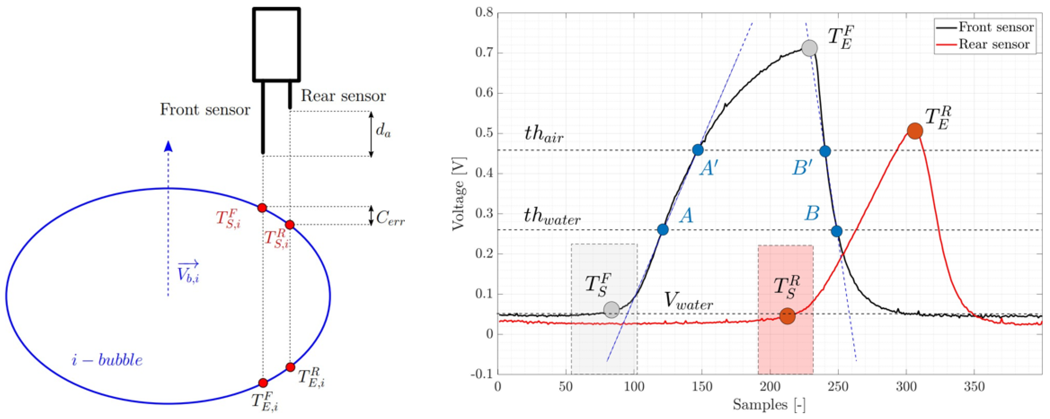
Figure 2.
Bubbly regime (example real trace). Top: full 5 s record from a conductivity probe at kHz showing dispersed, well-separated pulses. Bottom: magnified window highlighting variability in chord duration and rise/fall slopes; peak amplitudes differ due to bubble–probe contact geometry. Overlaid bands indicate expert-labeled gas intervals used as GT.
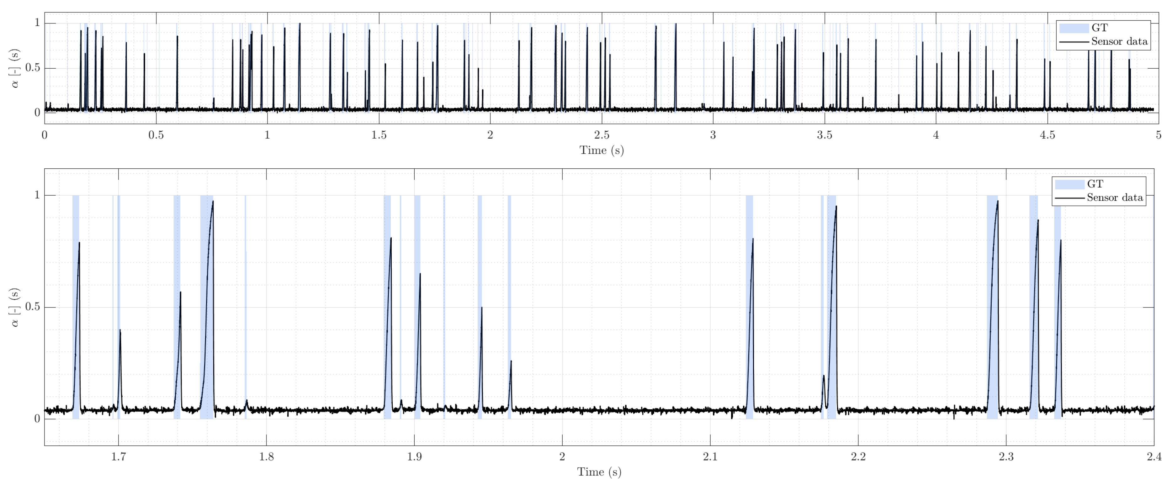
Figure 3.
Slug-like regime (example real trace). Top: full 5 s record with a Taylor-bubble plateau followed by dense bubble trains; baseline becomes locally ambiguous under sustained gas occupancy. Bottom: detail view showing clustered transients and short liquid gaps. Overlaid bands indicate expert-labeled gas intervals used as GT.
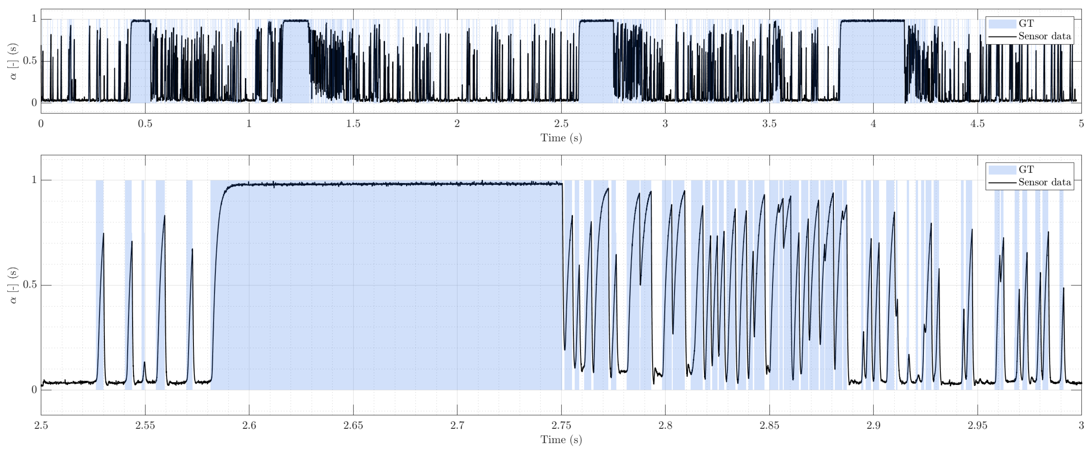
Figure 4.
Hand-labeled bubbly slopes from multiple sensors, min–max normalized and aligned at the half-height crossing, together with logistic fits at different steepness values
Figure 4.
Hand-labeled bubbly slopes from multiple sensors, min–max normalized and aligned at the half-height crossing, together with logistic fits at different steepness values
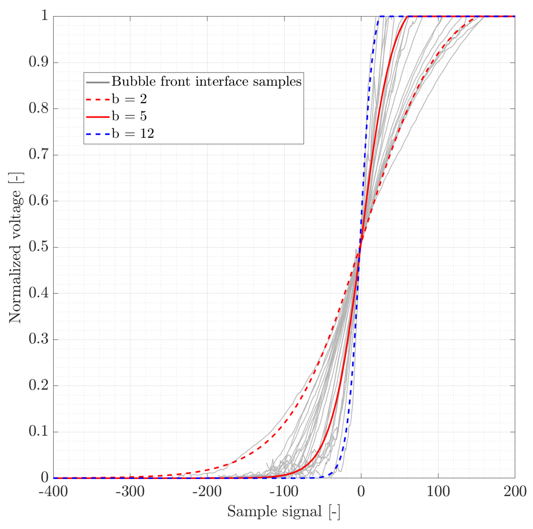
Figure 5.
Examples of synthesized trace resembling slug flow conditions (top) and bubbly flow conditions (bottom) with its corresponding binary exact GT.
Figure 5.
Examples of synthesized trace resembling slug flow conditions (top) and bubbly flow conditions (bottom) with its corresponding binary exact GT.
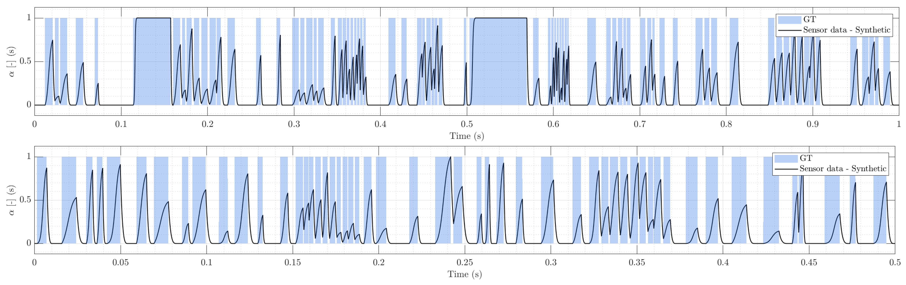
Figure 8.
Sample from a real signal of a conductivity-local probe and its GT obtained by human expert-labeling used to evaluate proposed models.
Figure 8.
Sample from a real signal of a conductivity-local probe and its GT obtained by human expert-labeling used to evaluate proposed models.
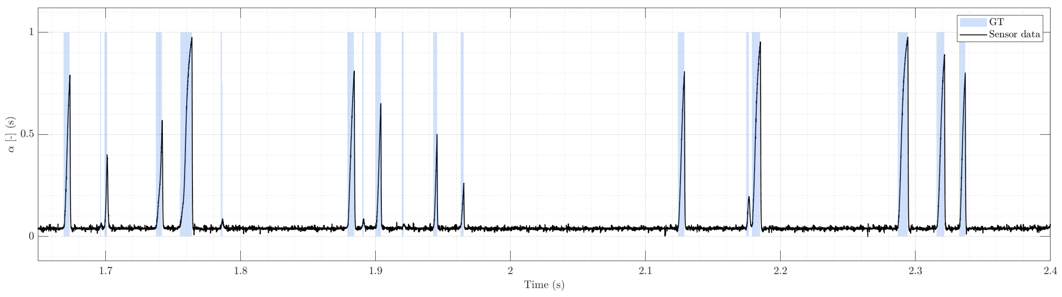
Figure 9.
Detail of bubbly flow signal evaluation: Threshold-based methods (top) and DL models inferences (bottom).
Figure 9.
Detail of bubbly flow signal evaluation: Threshold-based methods (top) and DL models inferences (bottom).
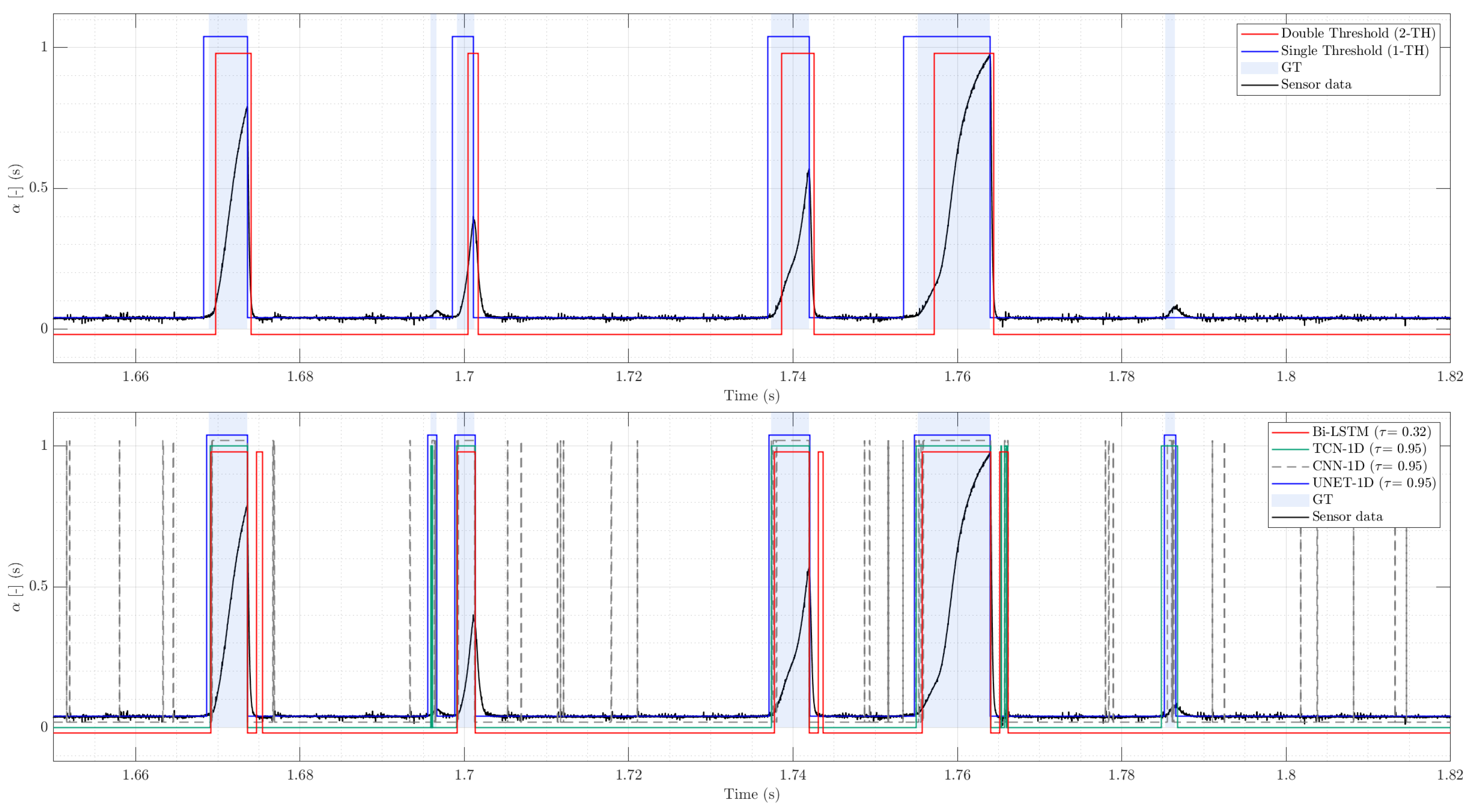
Figure 10.
Detail of slug flow signal evaluation: Threshold-based methods (top) and DL models inferences (bottom).
Figure 10.
Detail of slug flow signal evaluation: Threshold-based methods (top) and DL models inferences (bottom).
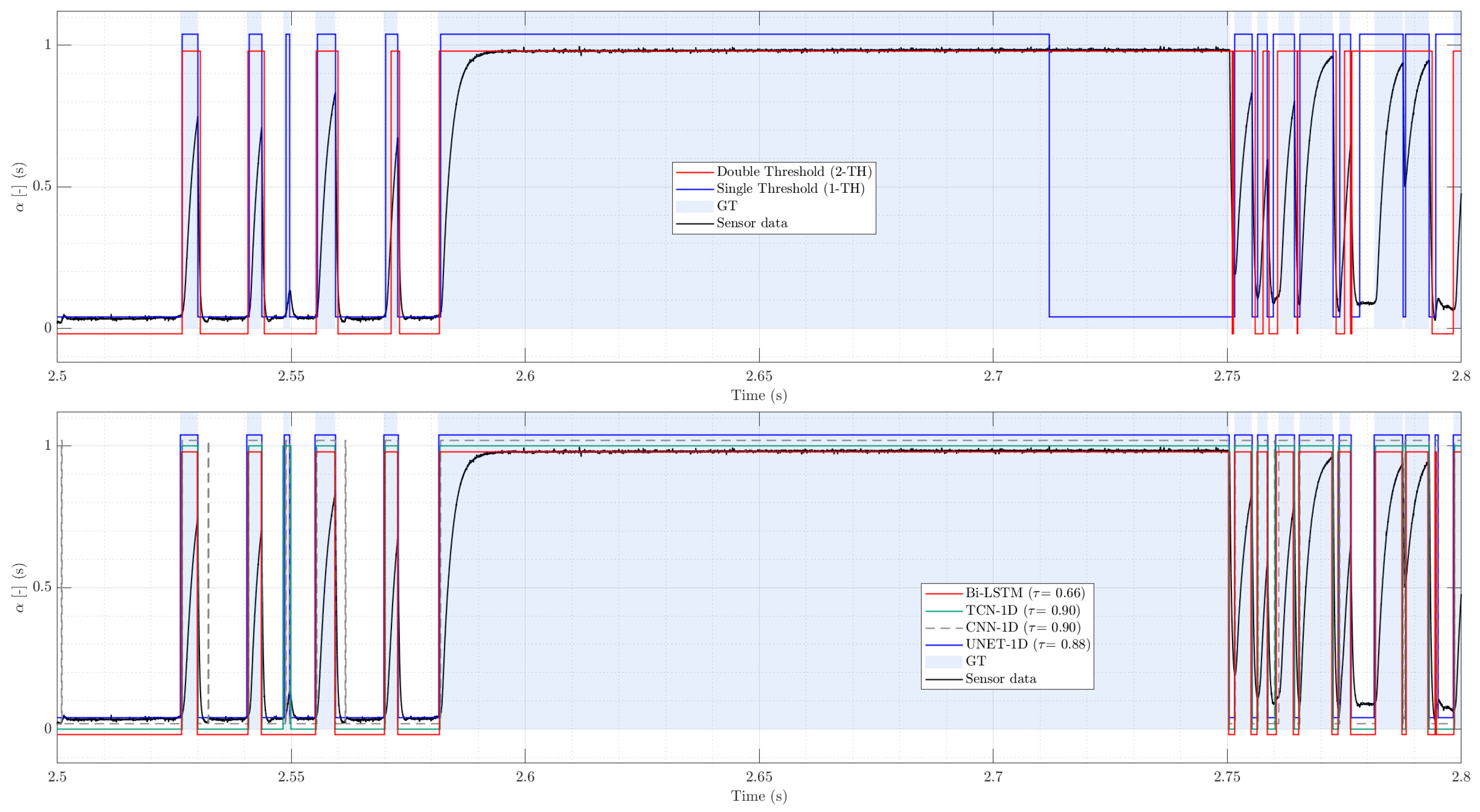
Figure 11.
Detail of bubbly flow signal with superimposed baseline oscilation signal: Test signal example (top) and threshold-based methods and UNET-1D model inferences (bottom).
Figure 11.
Detail of bubbly flow signal with superimposed baseline oscilation signal: Test signal example (top) and threshold-based methods and UNET-1D model inferences (bottom).
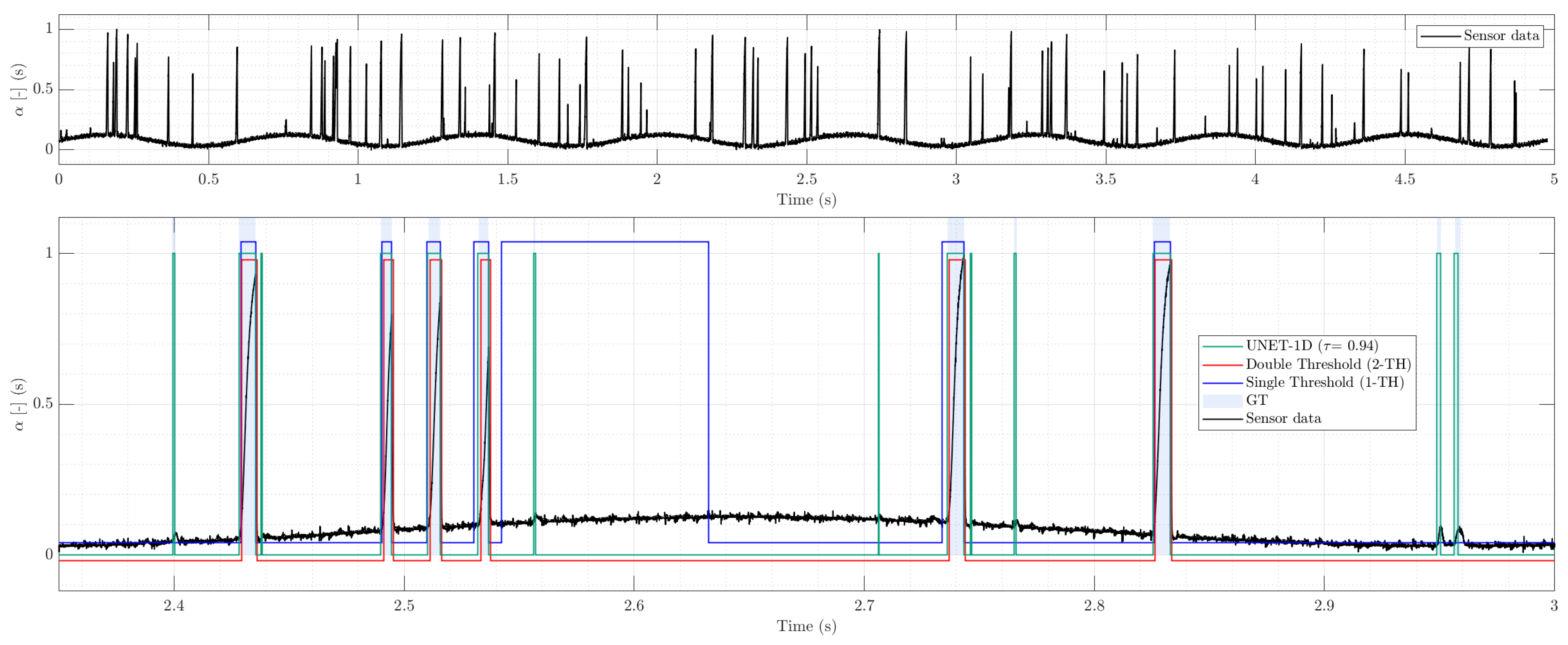
Figure 12.
Detail of slug flow signal with superimposed baseline oscilation signal: Test signal example (top) and threshold-based methods and UNET-1D model inferences (bottom).
Figure 12.
Detail of slug flow signal with superimposed baseline oscilation signal: Test signal example (top) and threshold-based methods and UNET-1D model inferences (bottom).
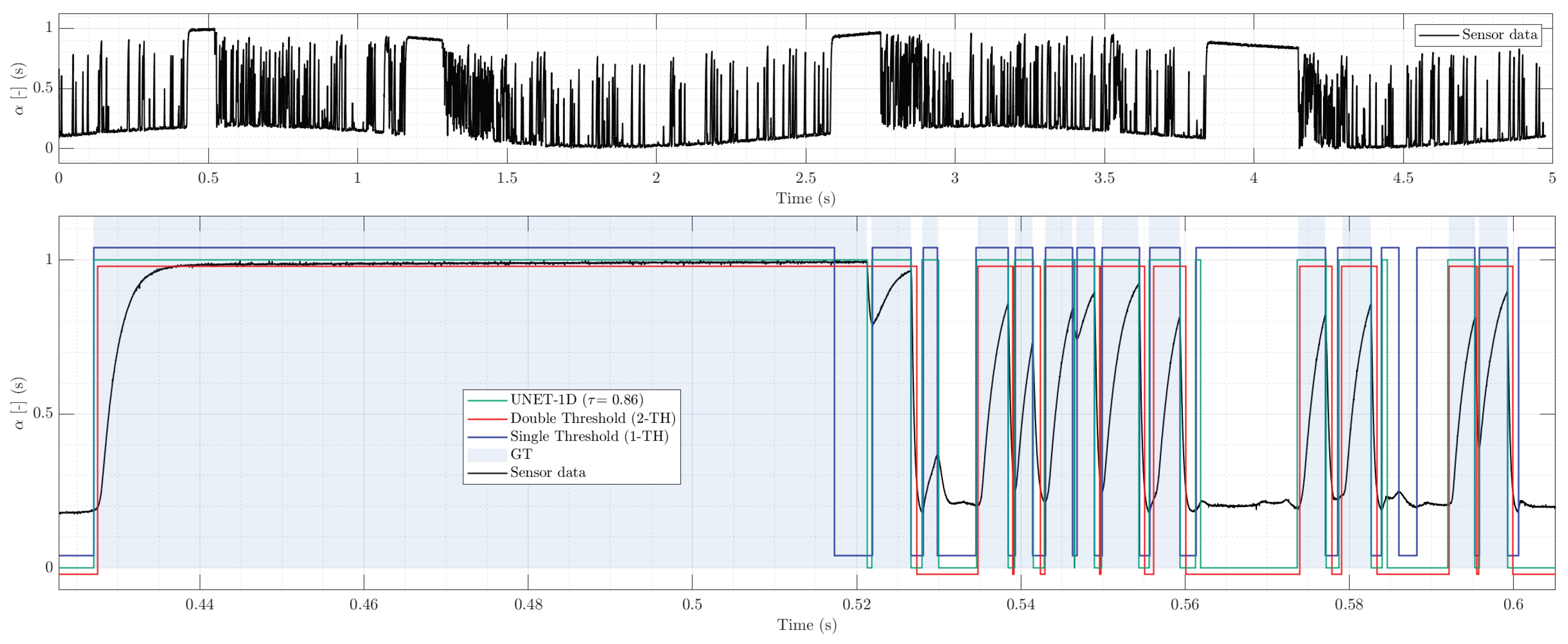

Table 1.
Metrics for the synthetic signal evaluation (=0.5035, =129).
| Method | MAE | P95 | COV | OVL | TP | FP | FN | ||||
|---|---|---|---|---|---|---|---|---|---|---|---|
| [-] | [ms] | [ms] | [-] | [-] | [-] | [-] | [-] | [-] | [-] | [-] | |
| 1-TH | 0.961 | 4.216 | 11.080 | 0.3349 | 0.0000 | 0.333 | -0.1709 | 125 | 122 | 3 | 7 |
| 2-TH | 0.617 | 7.286 | 14.000 | 0.2333 | 0.0391 | 0.270 | -0.2330 | 85 | 66 | 19 | 63 |
| UNET-1D | 0.989 | 1.105 | 2.500 | 0.5030 | 0.0284 | 0.531 | 0.0279 | 132 | 129 | 3 | 0 |
| TCN | 1.000 | 1.151 | 3.520 | 0.5036 | 0.0229 | 0.523 | 0.0193 | 129 | 129 | 0 | 0 |
| Bi-LSTM | 0.988 | 1.767 | 7.150 | 0.4462 | 0.0049 | 0.451 | -0.0524 | 128 | 127 | 1 | 2 |
| CNN-1D | 0.996 | 0.221 | 0.400 | 0.5019 | 0.0054 | 0.507 | 0.0038 | 130 | 129 | 1 | 0 |
Table 2.
Metrics for the contaminated bubbly flow signal test (=0.0838, =109).
| Method | MAE | P95 | COV | OVL | TP | FP | FN | ||||
|---|---|---|---|---|---|---|---|---|---|---|---|
| [-] | [ms] | [ms] | [-] | [-] | [-] | [-] | [-] | [-] | [-] | [-] | |
| 1-TH | 0.294 | 1.915 | 3.926 | 0.0828 | 0.6621 | 0.729 | 0.646 | 88 | 29 | 59 | 80 |
| 2-TH | 0.785 | 0.911 | 1.619 | 0.0589 | 0.0089 | 0.066 | -0.0174 | 72 | 71 | 1 | 38 |
| UNET-1D | 0.926 | 0.254 | 0.550 | 0.0830 | 0.0077 | 0.089 | 0.0050 | 122 | 107 | 15 | 2 |
| TCN | 0.800 | 0.314 | 0.632 | 0.0802 | 0.0060 | 0.084 | 0.0005 | 151 | 104 | 47 | 5 |
| Bi-LSTM | 0.714 | 0.476 | 0.931 | 0.0835 | 0.0708 | 0.151 | 0.0674 | 174 | 101 | 73 | 8 |
| CNN-1D | 0.128 | 1.397 | 3.953 | 0.0742 | 0.0133 | 0.087 | 0.0037 | 1573 | 108 | 1465 | 1 |
Table 3.
Metrics for the contaminated slug flow signal test (=0.4208, =524).
| Method | F1evt | MAE | P95 | COV | OVL | TP | FP | FN | |||
|---|---|---|---|---|---|---|---|---|---|---|---|
| [-] | [ms] | [ms] | [-] | [-] | [-] | [-] | [-] | [-] | [-] | [-] | |
| 1-TH | 0.905 | 0.617 | 1.850 | 0.284 | 0.0251 | 0.309 | -0.1118 | 455 | 443 | 12 | 81 |
| 2-TH | 0.786 | 0.771 | 2.061 | 0.341 | 0.0427 | 0.383 | -0.0377 | 344 | 341 | 3 | 183 |
| UNET-1D | 0.952 | 0.190 | 0.700 | 0.409 | 0.0165 | 0.425 | 0.0038 | 501 | 488 | 13 | 36 |
| TCN | 0.928 | 0.372 | 1.769 | 0.402 | 0.0221 | 0.424 | 0.0030 | 478 | 465 | 13 | 59 |
| Bi-LSTM | 0.850 | 0.402 | 2.045 | 0.388 | 0.0257 | 0.413 | -0.0075 | 450 | 414 | 36 | 110 |
| CNN-1D | 0.834 | 0.899 | 3.245 | 0.369 | 0.0058 | 0.374 | -0.0465 | 661 | 494 | 167 | 30 |
Table 4.
Metrics for the bubbly flow case evaluation (=0.0838, =109).
| Method | MAE | P95 | COV | OVL | TP | FP | FN | ||||
|---|---|---|---|---|---|---|---|---|---|---|---|
| [-] | [ms] | [ms] | [-] | [-] | [-] | [-] | [-] | [-] | [-] | [-] | |
| 1-TH | 0.912 | 0.329 | 0.845 | 0.0792 | 0.0055 | 0.083 | -0.0009 | 95 | 93 | 2 | 16 |
| 2-TH | 0.785 | 0.884 | 1.299 | 0.0593 | 0.0089 | 0.067 | -0.0171 | 72 | 71 | 1 | 38 |
| UNET-1D | 0.939 | 0.231 | 0.454 | 0.0833 | 0.0069 | 0.088 | 0.0045 | 119 | 107 | 12 | 2 |
| TCN | 0.817 | 0.288 | 0.843 | 0.0814 | 0.0062 | 0.086 | 0.0019 | 143 | 103 | 40 | 6 |
| Bi-LSTM | 0.723 | 0.476 | 0.775 | 0.0843 | 0.0824 | 0.163 | 0.0796 | 173 | 102 | 71 | 7 |
| CNN-1D | 0.173 | 1.474 | 3.905 | 0.0744 | 0.0071 | 0.082 | -0.0023 | 1136 | 108 | 1028 | 1 |
Table 5.
Metrics for the slug test (, ).
| Method | F1evt | MAE | P95 | COV | OVL | TP | FP | FN | |||
|---|---|---|---|---|---|---|---|---|---|---|---|
| [-] | [ms] | [ms] | [-] | [-] | [-] | [-] | [-] | [-] | [-] | [-] | |
| 1-TH | 0.949 | 0.332 | 0.775 | 0.3153 | 0.0088 | 0.3236 | -0.0972 | 483 | 478 | 5 | 46 |
| 2-TH | 0.801 | 0.690 | 1.823 | 0.3569 | 0.0745 | 0.4307 | 0.0099 | 355 | 352 | 3 | 172 |
| UNET-1D | 0.954 | 0.187 | 0.675 | 0.4085 | 0.0158 | 0.4237 | 0.0029 | 503 | 490 | 13 | 34 |
| TCN | 0.936 | 0.375 | 1.499 | 0.3988 | 0.0188 | 0.4170 | -0.0038 | 482 | 471 | 11 | 53 |
| Bi-LSTM | 0.890 | 0.595 | 2.000 | 0.3996 | 0.0524 | 0.4520 | 0.0312 | 442 | 430 | 12 | 94 |
| CNN-1D | 0.827 | 0.848 | 3.311 | 0.3886 | 0.0090 | 0.3969 | -0.0239 | 687 | 501 | 186 | 23 |
Disclaimer/Publisher’s Note: The statements, opinions and data contained in all publications are solely those of the individual author(s) and contributor(s) and not of MDPI and/or the editor(s). MDPI and/or the editor(s) disclaim responsibility for any injury to people or property resulting from any ideas, methods, instructions or products referred to in the content. |
© 2025 by the authors. Licensee MDPI, Basel, Switzerland. This article is an open access article distributed under the terms and conditions of the Creative Commons Attribution (CC BY) license (http://creativecommons.org/licenses/by/4.0/).
Copyright: This open access article is published under a Creative Commons CC BY 4.0 license, which permit the free download, distribution, and reuse, provided that the author and preprint are cited in any reuse.


