
Submitted:
12 November 2025
Posted:
13 November 2025
You are already at the latest version
Abstract
We investigate the planar Dirac equation with the most general time-independent contact (singular) potential supported on a circumference. Taking advantage of the radial symmetry, the problem is effectively reduced to a one-dimensional one (the radial), and the contact potential is addressed in a mathematically rigorous way using a distributional approach that was originally developed to treat point interactions in one dimension, providing a physical interpretation for the interaction parameters.
The most general contact interaction for this system is obtained in terms of four physical parameters: the strengths of a scalar and the three components of a singular Lorentz vector potential supported on the circumference. We then investigate the bound and scattering solutions for several choices of the physical parameters, and analyze the confinement properties of the corresponding potentials.
Keywords:
dirac equation
; contact potentials
; eigenstates
; scattering states
1. Introduction
Much work has recently been done on the role of electric and magnetic fields for technological applications in the confinement of relativistic massive charged particles, especially in two-dimensional systems governed by the Dirac-Weyl equation [1,2,3,4,5,6,7,8,9,10,11,12,13,14,15,16], although it is known that this is not suitable for massless two-dimensional particles due to the existence of a strong Klein tunneling effect [17,18]. Another situation where electric fields are able to confine particles is when we deal with a quantum dot with some kind of symmetry, typically radial, that allows for a well-defined angular momentum quantum number. Confinement of massive particles in two dimensions has also been studied to better understand new topological materials, such as graphene, silicene, germanene, stanene and phosphorene [19,20,21], where charges acquire effective mass from spin-orbit interaction and perpendicular electric fields [22,23]. An important consequence of massive particle confinement is that it allows to observe the phenomenon of atomic collapse, which is very difficult to detect in relativistic quantum mechanics but is accessible with Dirac materials [24,25,26,27] due to the existence of the Fermi velocity [28]. The search for resonances is also an interesting topic, and in fact confinement in Dirac materials must necessarily include bound and resonance states [29].
Although it is clear that the aforementioned technological applications are extremely interesting, in this work our focus will be on the theoretical analysis of certain two-dimensional systems that are governed by the (2+1) massive Dirac equation subjected to a type of toy potentials, the singular contact interactions in two dimensions. It is well known that contact or point interactions in one-dimensional relativistic quantum mechanics have been used to model short-range potentials. They are singular interactions whose appropriate treatment needs the use of special mathematical methods in order to avoid ambiguities (see [30] and references quoted therein). The main goal of the present work is to adapt a recent distributional approach, originally developed for the one-dimensional case [31], to study, in a mathematically rigorous manner, radially symmetric two-dimensional contact interactions supported on a circumference of radius R. From the radial symmetry it is possible to reduce the problem to one dimension (the radial one), and apply in an almost straightforward way the distributional approach of [31] to a contact potential at . In the actual one-dimensional case, the usual four parameters of the point interactions can be rewritten in terms of four physical potentials strengths, corresponding to a scalar, a pseudoscalar and the two componentes of a (1+1) Lorentz electromagnetic point potential [31]. As it will be seen here, in the two-dimensional case with radial symmetry and a singular potential concentrated on a circumference, those four parameters will correspond to the physical strengths of a scalar and the three components of a (2+1) electromagnetic Lorentz singular potential. After obtaining the general solutions for the Dirac equation with the most general contact interaction concentrated on the circumference, we will consider some special cases, namely a purely scalar potential, a purely electrostatic potential, a purely magnetic potential and two mixtures of a scalar and an electrostatic potential. In each of these cases we will systematically investigate the confining properties of the contact potential, understood broadly as the structure of the bound states and resonances, and the conditions under which the circular barrier becomes impenetrable.
The structure of the paper is as follows. In Section 2 we review the covariant form of the Dirac equation in (2+1) dimensions with the most general external regular potential with radial symmetry. In Section 3 we consider the (2+1) Dirac equation with the most general, time-independent, contact potential supported on a circumference of radius R. In Section 4 we determine the equations for the energy eigenstates of the previously derived Dirac radial equation, including bound states, scattering states, and resonances. These quantities are subsequently investigated for some special cases of physical interest in Section 5. The paper ends with a discussion and conclusions in Section 6.
2. Planar Dirac Equation with a Radial Regular Potential
In this section we briefly review the covariant form of the Dirac equation in (2+1) dimensions with the most general external regular potential1, which is formed by a scalar and a vector potential , with and (we are using natural units, ):
For convenience, we will use the following representation of the Dirac matrices, in terms of the Pauli matrices:
We are interested in the case where in a particular reference frame (e.g. the laboratory frame) the potentials are independent of time, and the time-independent Dirac equation reads as follows:
where is the position vector of the Dirac particle in the cartesian coordinates of the laboratory frame, is the corresponding time independent Dirac spinor and
Even if the potential in the Dirac equation (3) is , we will sometimes abuse the language and will refer to as the potential.
Since we are only interested in the case where the potentials have radial symmetry (in the laboratory reference frame), it is natural to use polar coordinates from now on. The space cartesian components () of the Lorentz vector potential transform to the polar components and , with and the polar angle, as:
where , , and, with a slight abuse of notation, , . By defining
we can write (4) in polar coordinates as
The whole potential will have radial symmetry if all the above four potentials , , and depend only on r, and in this case we will denote them simply as and .2 Thus, in polar coordinates the Dirac equation (3), with a radial potential (7), reads3
Taking advantage of the radial symmetry, we seek for solutions of the time independent Dirac equation that are also eigensolutions of the total angular momentum operator:
By writing the time independent Dirac spinor in the separated form
where and , the eigenvalue equation for is , which implies
and, thus,
It is direct to see that is a unitary matrix, .
Now, turning (10), with (11), into the Dirac equation (8), and multiplying from the left by , we obtain
From (11), (6) and (2) we have
Substituting the above results into the equation (12), we obtain the radial Dirac equation
which can be written in terms of an effective potential:
where
Conservation of the Dirac Current
The Dirac current in (2+1) dimensions, in cartesian components, is given by
The current conservation states that , which, in the cartesian coordinates of the laboratory frame, reads as
Integrating the above on a arbitrary circle of radius , and using the divergence theorem, we obtain (below, is the unit vector in the radial direction):
where is the total probability to find the Dirac particle enclosed inside the circumference of radius . Above, we identified the radial component of the Dirac current, , and used the fact that the radial symmetry implies that it does not depend on (see below).
Now we restrict ourselves to the stationary case. From the radial symmetry, we have
The explicit form of the component is
and, for the cartesian space components, we have
where, from (6) and (20), we have identified the r and -components of the stationary Dirac current as
From (21) and (22) it is clear that both the current’s polar components and do not depend on the angular coordinate , as mentioned earlier. Thus, we write and . From the above we have that along the angular direction both the stationary currents and are constant and, from (19), in the stationary case we have that the quantity vanishes, which implies that , . In particular, for any radius :
Summarizing the results obtained so far, we have that, for an external, regular, and radial symmetric potential, , the radial spinor must solve the one-dimensional stationary Dirac equation (15) with the effective one-dimensional potential (16). Conservation of the Dirac current in the original two-dimensional problem implies that the one-dimensional (radial) stationary current , given by (21), is continuous (and vanishes) at any r, and therefore satisfies condition (23).
Equation (15) is mathematically analogous to the Dirac equation in (1+1) dimensions, with an external potential (see Equation (3) at p. 4 of [31]). However, (15) holds only for . In the next Section we will see how to extend it as a distributional equation on the interval , and which condition the Dirac spinor must satisfy at . The analogous roles of the potentials and of the regular, true one-dimensional case (see the Equation (2) of [31]) will be played in (15) by the following combinations
It is worth to observe that in (15) the effective one-dimensional potential in the radial direction, , is not Hermitian, due to the presence of the imaginary quantity added to the potential in (24). However, this is immaterial, since for the distributional method of [31] to be applicable in the present case it suffices that the current be continuous at . Finally, it is worth to note that the original potential is in fact Hermitian, and the Lorentz vector is conserved.
3. Dirac Equation with Radial Contact Potentials at
Now we consider the Dirac equation with the most general, time-independent, contact potential supported on a circumference of radius R in the laboratory frame. Since now the potential is singular, the products between the potentials and the spinors appearing in (15) are not well defined. Guided by the analogy to the one-dimensional case, we follow closely the steps of reference [31] and write the time independent Dirac equation as
where
is the regular part of the effective potential. Since this term defines a regular distribution on , which includes the origin, the equation (25), understood as a distributional equation, can be extended to include the origin, which will be assumed from now on.4 The first term in the right hand side of (25) is the contact term, and is a matrix, yet unknown, whose elements are singular (not regular) distributions, related to the singular potentials concentrated at . The distribution space we consider here is the Schwartz space , which consists of continuous linear functionals acting on the Schwartz space of infinitely differentiable strongly decreasing test functions. For details, we refer the reader to reference [31]. The distribution will be determined from the following three basic requirements (adapted from [31]):
- (R1)
- must be a distribution concentrated at , i.e., it must equals the zero distribution in .
- (R2)
- The two components of the radial Dirac spinor must correspond to regular distributions on , i.e., they must be slow growth functions and locally integrable (in the Lebesgue sense) on . This is equivalent to saying that must have order on any closed interval .
- (R3)
- The Dirac current must be conserved across . In the stationary case this implies that .
The definition we are using above for the order of a distribution on a closed, finite interval , is the same of [31], adapted to the semi-infinite axis . Briefly, with , the order of the Dirac delta distribution on K is . Taking the derivative of any distribution increases its order on K by , whereas taking an indefinite integral (a primitive) decreases its order by . The order of a sum of distributions on K is the largest order of its terms. A distribution has order on K if it is infinitely differentiable on K. A distribution has order on K if on this interval it coincides with a continuous but not differentiable (in the ordinary sense) function. A distribution of order corresponds to a discontinuous function, and may or may not be regular. A distribution having order on K is always singular. For more details, we refer the reader to [31].
From requirement (R2), and balancing the orders on both sides of (25), the order of the interaction distribution on any interval must be . This same requirement also sets a maximum for the order of the spinor on a closed finite interval containing the origin, but not containing R, i.e., , . Since on the contact distribution equals the zero distribution, and the term (26) has order (since it is regular on , see footnote 4), by balancing the orders on both sides of (25) we conclude that on and, consequently, on . This means that the spinor must be continuous on and, therefore, it must be bounded at the origin.5 This is another way to justify, in a mathematically rigorous way, the usual assumption of boundedness of the Dirac spinor at .
Theorem 3.5-2 of [32] states that a distribution that is concentrated at a single point , and that has singular order s on a closed finite interval , must in this interval coincide with a finite linear combination of Dirac deltas and its derivatives, up to order s. Since on K the order of is zero, we must have . We have that, on K, (from (R2)) and, consequently, . Now, by balancing the orders on both sides of (25), we have that , and therefore on K. Requirements (R1) and (R2) thus imply that
where the matrix does not depend on the coordinate r, and will have a functional (linear) dependence of the spinor . The form of will completely specify the contact term, and below it will be found from requirement (R3). As will be shown, the obtained form of will imply matching conditions that must satisfy at , similar to the true one-dimensional case. Also, it will provide the contact term explicitly as a well defined distribution defined on the semi-axis .
To determine we proceed exactly in the same way as in [31]. By taking a distributional indefinite integral of equation (25) on , , we obtain
where is any primitive of , is a primitive of the product and c is a constant and arbitrary column matrix. Similarly to the reasoning in [31], we conclude that both functions, and , are continuous on K.6 By isolating the term in the above equation, we find that must have well defined lateral limits at . By considering the limits in (28) and taking the difference, we obtain:
Now the functional coefficient will be determined from requirement (R3):
The problem of determining from (29), by using the current condition (30), is mathematically analogous to the one-dimensional problem treated in [31]. Therefore, we just collect the results from [31], replacing the analogous quantities to the present problem:
where the real constants and are identified with the strengths of the singular potentials associated to the contact term supported on , namely, from (27)
The radial Dirac equation (25), with the contact and the regular interaction terms given explicitly, is:
A permeable contact interaction is characterised by the condition (see Equation (55) of [31])
which means that the solutions at and are connected by the following matching conditions
where the matrix is written in terms of the physical strengths as7
Yet, to have a unique set of -parameters , given a set of parameters and and satisfying the permeability conditions (34), we can write the relationships:
where in the above expressions the plus (minus) sign must be taken if (); if we must take the same sign of (see [31]).
When the strength potentials are such that the permeability condition (34) is not met, the circular wall at is impenetrable, and some (or all) of the matrix parameters becomes infinite. In this case, the inner and outer solutions are independent, the (anti)particle is completely confined in the inner (outer) region of the circumference of radius R, and it cannot be transmitted to the outer (inner) region. The set of allowed energies for the (anti)particle confined in the inner region will depend on the boundary conditions at , which in turn depend on the values of the strength potentials. In the outer region all energies are allowed; the cases may or may not be allowed in the outer region, as we will see later. In the following sections, we will use the matching conditions (35), together with the form (36) of the matrix in terms of the physical strengths, to study bound, scattering, and resonant states for various choices of the contact potentials. Cases that give rise to an impermeable wall can be obtained by considering the corresponding limits on the parameters.
4. Energy Eigenstates
In this section we will determine the energy eigenstates for the radial Dirac equation (15), for a given angular momentum . Consider the spinorial form of the solutions, for the inner (, ) or the outer (, ) regions
The spinors are solutions of equation (14), with (the free equation). In terms of the spinor components , , , that equation reads
When , by isolating from the first of equations (41) and substituting it into the second equation, we obtain a Schrödinger-like equation for , valid ,
where we defined . The solution of (42) is (see equation (2.13) of [33])8
where () and () are, respectively, the Bessel (Hankel) functions of the first and of the second kind. Substituting this solution into the first of equations (41), we obtain (see also [33]):
Thus, the radial part of the energy and angular momentum eingenstates (40) of the free Dirac particle in the inner and outer regions can be written in the form
Since the inner solution must be bounded at the origin (see the discussion regarding requirement (R2) in Section 4), and this holds only for the spinor whose elements are Bessel functions of the first kind, from now on we will consider only the first line of equations (45), with , as the solution for the inner region.
4.1. Critical and Supercritical States ()
The states for which or are called, respectively, critical and supercritical states and are important since, as we will see later, by varying the strengths of the potential a resonance can transform into a bound state, and vice versa. In the former case we say that a bound state is captured (or absorbed) from the continuum, and in the latter, that a bound state was emitted into the continuum. Captures or emissions of bound states from and to the continuum always occur at a critical or supercritical energy. To solve the Dirac equation for these states we must consider the equation (41) with .
4.1.1. Critical States
The critical states () solve the equation (42), with (an Euler equation),
and the first of equations (41), with :
The solutions of (46) have the form , but since we only consider and require the Dirac spinor be bounded at , only the solution is admissible in the inner region. We also require the Dirac spinor to be bounded at infinity (a physical requirement), so the only admissible solution for the outer region is . Therefore, the solutions for (46) in the inner and outer regions are
with and being arbitrary constants. substituting these solutions into (47), we obtain and . Therefore, the solutions for critical states in the inner and outer regions are
These two solutions must match at using the matrix , according to (35),
that results in
This equation has non-trivial solutions for if, and only if, the following secular equation is satisfied by the parameters of the matrix
From (49) we observe that critical states with are not true bound states: they are quasi-bound states, since they are bounded or vanish at infinity, but are not square integrable.9 For the critical states are true bound states.
4.1.2. Supercritical States
To obtain the supercritical states () we isolate in the second of the equations (41) and substitute it in the first, obtaining another Euler equation
whose solutions are of the form . Similarly to the previous case, for the inner region the solution with the positive sign is the only admissible one, while for the outer region we need only consider the solution with the negative sign. The corresponding solutions for are obtained from the second of the equations (41). Therefore, the admissible supercritical solutions in the inner and outer regions are
Again, to match solutions at we use (35), , and we obtain the following secular equation for the existence of non-trivial solutions:
From (54) we observe that, with the exception of , the supercritical states correspond to true bound states. Let us emphasize that the phase factor of the matrix does not enter the conditions (52) and (55) for the existence of critical or supercritical states.
4.2. Bound States ()
The bound states are characterized by , and in this case , with . For the outer region, it is more convenient to consider the solution in terms of Hankel functions, since it is easier to explore their asymptotic behavior as . The Hankel functions behave asymptotically as
From the above we see that the Hankel function explodes as r goes to infinity, while gives an evanescent wave. So, for bound states, we must have in the second line of equations (45). The inner and outer solutions must be matched at by using (35) :
that gives
where is the matrix whose columns are
The condition for (58) to have non-trivial solutions for the coefficients and is that . By writing , where the superscript T denotes the matrix transpose, we obtain the secular equation for the bound state energies:
From the above equation we observe that the phase factor of the matrix again does not affect the energies of the eventual bound state. In terms of the matrix parameters, the above equation may be written as as
where and represent the modified Bessel functions of the first and second kinds, respectively. Again, the above secular equation can be written in terms of the physical parameters B and () using (38)-(39).
4.3. Scattering States ()
The scattering states correspond to energies , such that . The outer solution, written in terms of the Bessel functions of the first and second kinds, is given by (45):
The asymptotic behavior of these Bessel functions, that is,
suggests the following way of writing the coefficients , in terms of the phase shift :
where h may be complex, but is real. Therefore,
and the matching condition (35) at gives
where we have represented the columns of the left-hand side matrix as column matrices. To obtain non-trivial solutions for , the determinant of the matrix on the left-hand side must be zero. Expressed in terms of the matrix parameters, this requirement results in the following expression for the phase shift :
From the above expression we can calculate the Wigner time delay [34]
which gives us a scale for the time the particle spends in the inner region . The above equations for the phase shift and the Wigner time delay do not depend on the phase factor of the matrix and again these expressions can be expressed in terms of the physical parameters using (38)-(39).
4.4. Resonances
A very practical method for investigating resonances is to look for the energies at which the scattering states become purely outgoing states. Of course, it is not physically possible to have only purely outgoing scattering states, and for this we need to search for complex energies. The real part of these complex energies will correspond to the resonances. Although not physically possible, purely outgoing scattering states contain important information about the system: in addition to giving the resonant energies, the inverse of the imaginary parts of these complex energies provides scales for the corresponding resonant time delays, as we will see later [33].
A second, more physical way to characterize the resonant energies of the scattering states is to associate them with the peaks of the Wigner time delay at (67). This is quite intuitive, since resonant states are associated with larger amounts of time that the particle spends within the inner region . We will later show, in the context of the special cases investigated, that these two criteria give in general the same values for the resonances.
To identify the outcoming and incoming scattering states, it is convenient to write the scattering solution in the external region in terms of the Hankel functions (the second line of equations (45)). We can use the asymptotic behavior of the Hankel functions (56), with , to identify the outcoming and incoming scattering solutions as and , respectively. Thus, the purely outcoming solutions will have only the Hankel function of the first kind , and thus we put in (45). The secular equation will then be exactly the same as we obtained previously for the bound states, i.e., equation (61), but now with , and we look for solutions of that equation for the complex energy . Obviously, all solutions for a real energy in the interval will be included in the set of complex solutions, and these will correspond to the bound (or quasi-bound) states.
As we continuously change the potential strengths and (or, equivalently, the parameters of the matrix ), new bound states can be created (captured from the continuum) or destroyed (emitted into the continuum). A capture(emission) generally occurs when the energy of a previous resonant(bound) state continuously crosses the (super)critical values , becoming a new bound(resonant) state. The values of the potential strengths (or parameters) for which a capture or emission from or to a bound state occurs are given by the conditions (52) and (55) for critical () or supercritical () states, respectively.
5. Special Cases
In this section, we investigate some special cases of physical interest, where we choose the set of parameters motivated by the physical potentials singular at that we want to describe, according to the relations (37)-(39). For each case we systematically investigate the confinement properties of the circular potential (i.e., whether it admits bound states or is impermeable), as well as the structure of the resonances and the process of capture and emission of bound states. In all cases, we proceed as follows. First we obtain the values of the potential strengths corresponding to the critical and supercritical states, as well as the secular equation relating these strengths to the bound states energies. Next, we consider complex-energy solutions for purely outgoing scattering states, for various values of the potential strengths, and graphically investigate the structure of the resonances and the discrete set of energies associated with impermeable circular walls at . Finally, we investigate the Wigner time delay for the scattering solutions and compare its peaks with the resonant energies calculated using the complex-energy method.
Next we will consider five types of contact potentials concentrated at , namely: (i) a purely scalar shell, (ii) a purely electrostatic shell, (iii) a purely magnetic shell, (iv) a “ shell", ad (v) a “ shell”.
5.1. A Purely Scalar Shell Potential
First, we consider the case of a purely scalar potential, and B arbitrary which models an infinite “kick" in the (anti)particle mass at . From (36), the parameters of the matrix are
The above relations are invariant under the transformation , except for a global sign, which does not affect the analysis of the critical, supercritical, bound states, or resonances. Then, for our purposes, it is sufficient to study the behavior of the system when . If , we have an impermeable wall, according to (34); in such cases, the boundary conditions at become and , with (see [31]).
5.1.1. Critical, Supercritical and Bound States
The condition (52) for critical states reads
For there is only the free solution . For the solutions are
Thus, a necessary condition for having critical states is . These two solutions are related to each other by the transformation . On the other hand, the condition (55) for supercritical states is
which is similar to the condition for critical states, changing . We will have supercritical states only for , and for the following two values of B
which are also related between themselves by the transformation , as they should be. From the previous results we observe that if for a value of B we have a critical state for the angular momentum l, for this same value of B we will have a supercritical state for the angular momentum .
The secular equation (61) for the bound states, with (68), becomes:
The relationship between the bound state energies and the strength of the pure scalar singular field B is shown in Figure 1, where it is observed that emission/absoprtion
of bound states at the critical and/or supercritical energies is only allowed for angular momenta in the range , as mentioned above. For , no bound states exist, regardless of the value of the scalar field strength B.
5.1.2. Resonances
The complex energy solutions for the secular equation (71) are shown in Figure 2 as colored dots, for various positive values of the scalar strength B in the interval , for , and . The blue curve represent the locus of the complex solutions to the imaginary part of equation (71), which does not depend on the strength B.
For the circular wall becomes impenetrable (with boundary conditions depending on the sign of B, as seen above), and all complex energy solutions become real, and correspond to the set of discrete energies admissible for an (anti)particle confined in the inner circle, except, in the case , for the point (in brown in the figure) with energy , which corresponds to a bound state confined in the outer region of the circle (this state vanishes identically in the inner region, and is decaying in the outer region, as can be seen using the boundary conditions for this case). In the figure we observe that as and decreases from 2 to 0 the complex energies move away from the real axis along the blue U-shaped curves. On the other hand, as increases in absolute value, the complex solutions move towards the real axis, with the absorption of the first bound state at when B reaches the value (red dots in the figure).
5.1.3. Wigner Time Delay
Equation (66), in terms of the parameter B of (68), becomes
from which the Wigner time delay is obtained from (67).
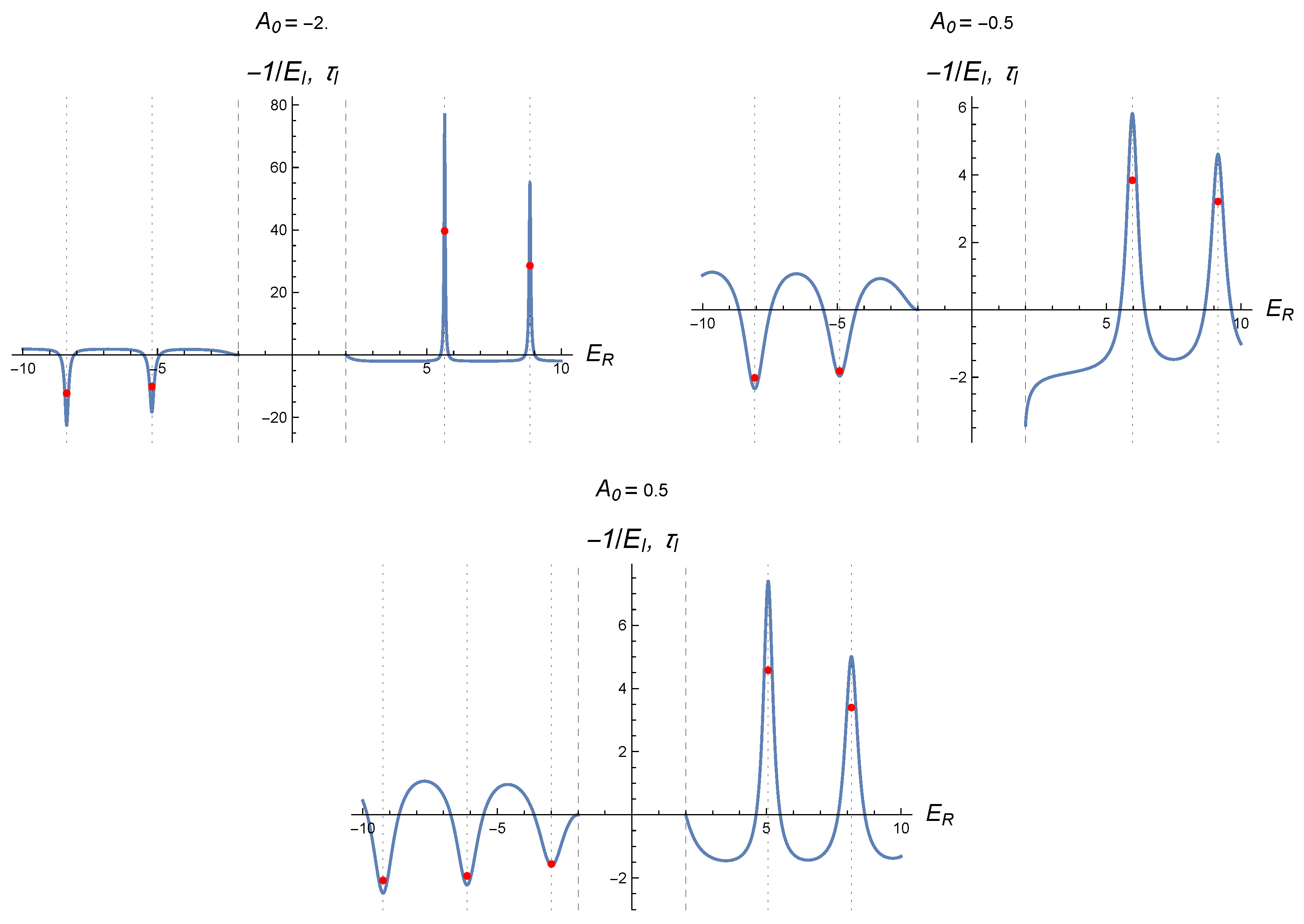
Figure 3 shows this time for some values of the parameter B. We observe very good agreement between the location of the sharp peaks (or valleys, in the case of negative energies) of the Wigner time delay and the real parts of the complex energies that solve (71). These plots also confirm that the negative inverse of the imaginary parts of the complex energies provides a scale for the Wigner time delay at the resonances.
5.2. A Purely Electrostatic Shell Potential
A purely electrostatic shell at will have , and an arbitrary . From (36), the parameters of the matrix in this case are
We note that the transformation converts , which is equivalent to multiplying the matrix in (35) by . As already mentioned, multiplying by a phase factor (in fact, by any constant factor) does not affect the results for bound states, resonances, or phase delay. Thus, it is sufficient to investigate those quantities for positive values of . We also note that there is no value of for which the circular wall is impermeable, since the permeability condition (34) always holds for a purely electrostatic potential. In the limit the circular wall becomes completely transparent, since , which is a phase times the matrix of the free case.10
5.2.1. Critical, Supercritical and Bound States
The equation (52) for critical states, written in terms of the electrostatic strength is For , this equation has only the trivial solution , which corresponds to the absence of interaction (free case). For , we have two solutions,
which are related to each other by the transformation . Similarly, the equation (55) for the supercritical states is whose solutions, for , are
that also shows the symmetry .
The secular equation (61) for the bound states is written as
expression in which we observe that any energy in the interval will be associated to a single bound state energy for exactly two values of . Figure 4 shows the relationship between the bound state energies and the value of the electric potential strength , for three values of the angular momentum l.
5.2.2. Resonances
We now look for complex energy solutions to the secular equation (75), which can be rewritten in a convenient form as:
Figure 5 shows by means of colored dots the complex energies that solve (76), for various positive values of the electrostatic strength and .
The blue curve represents the solutions for the real part of (76), which does not depend on the potential intensity . As increases in the positive direction, the complex energy solutions move along the blue curve from left to right. When crosses the value (74) with the minus sign ( in the figure), a bound state is captured (green dots in the figure) at ; when crosses the value (73) with the plus sign ( in the figure), a bound state is emitted at (brown dots in the figure).
5.2.3. Wigner Time Delay
The equation (66), for the pure electrostatic case, becomes
from which we can calculate the Wigner time delay using (67), shown in Figure 6 for some values of the parameter . Again, we can observe a very good agreement between the sharp peaks (or valleys if the energies are negative) of the Wigner time delay and the real parts of the complex energies that solve (76).
5.3. A Purely Magnetic Shell Potential
In this section we will consider a general pure magnetic potential (), where and are not simultaneously zero. From (36), the parameters of the matrix are
As mentioned above, the value of the phase and the choice of the sign in (77) are irrelevant to determining the energies of the critical, supercritical, bound states, and resonances, so we will only consider the negative sign in the equation above, which implies that . All the analysis of the magnetic potential will be carried out in terms of the parameter a, but, for clarity, let us consider some particular limits and their relationships with the physical intensities and . From (77) we have that (resp. ) if, and only if, and (resp. ), which are the cases for an impermeable circular barrier, according to (34). The case (the free case) corresponds to the limit when the strength or (or both) tend to infinity.
5.3.1. Critical, Supercritical and Bound States
The condition (52) for critical states in this case reads . For any value of a admits a critical state. For only an impenetrable wall with admits a critical state, which will be a state for a particle confined in the inner region of the circular wall, as can be seen by using the boundary conditions in this case, . On the other hand, the condition (55) for supercritical states is and, again, only an impermeable barrier with will admit a supercritical state. In this case, however, the supercritical state will not correspond to an antiparticle confined in , but in the external region . The secular equation (61), with parameters (77), becomes:
The above equation has no solution for bound state energies , for any , since is real and nonzero, and the right-hand side of the above equation is always negative. This result can be extended to the cases . For the case we arrive at the same conclusion, explicitly considering the boundary conditions for the impermeable barrier in this case (see above). In summary, a purely magnetic potential does not allow solutions with . However, as we will see later, an impenetrable wall with will admit a set of discrete energies with or for an (anti)particle confined in the inner circle . Similarly, an impenetrable wall with will have states confined in the inner circle for a discrete set of energies , for , and , for , as can be concluded using the appropriate boundary conditions in this limiting case, namely .
5.3.2. Resonances
Figure 7 shows the complex energies solving the equation (78), for various values of the parameter , and for . As mentioned above, the case (dark blue points in the figure) corresponds to an impermeable circular barrier with and . In this case, the purely real solutions of (78) correspond to the admissible energies for an (anti)particle confined in the inner region of the circular impenetrable wall (this set includes , but not , which corresponds to the energy of a particle confined in the outer region).
The two complex solutions close to correspond to remnant resonances. The case (purple dots), corresponding to , also produces an impenetrable circular wall (with boundary conditions on the wall different from those in the case ) and, moreover, presents a set of purely real energies corresponding to the set of discrete energies admissible for an (anti)particle confined in the inner region of the impenetrable wall. The system also presents two complex solutions, corresponding to remnant resonances close to . We note (not shown in the figure) that, for lower values of the angular momentum ( and , with the remaining parameters fixed), such remnant complex resonances at the limits and do not appear. In both cases of impenetrable walls, the solutions in the outer region admits a continuum of energies , as expected. For , does not belong to this continuum (it vanishes identically in the outer region), but does (the solution with vanishes trivially in the inner region).
5.3.3. Wigner Time Delay
The Wigner time delay (67) is shown in Figure 8 for the same parameters as in Figure 7. For large values of the resonant energies (real parts of the complex energies that solve the second equation in (78)), we observe a very good agreement between these energies and the locations of the sharp peaks (or valleys for negative energies) of the Wigner time delay. For these resonances, the plots also confirms that the negative inverse of the imaginary parts of the complex energies gives a scale for the Wigner time delay. In the figure, the agreement between the real and imaginary parts of the complex energies and respectively the location and magnitude of the Wigner time delay peaks is poorer for low values of , and these relationships are absent for the two complex resonances close to . The lack of such correspondence may be understood from the fact that such resonances do not evolve to a confined state for the corresponding impenetrable barrier in the limits .
5.4. A “Delta Shell" Potential
The delta shell potential corresponds to an equal mixture of the scalar and the electrostatic potentials, with the magnetic potentials vanishing (arbitrary , ). We call it a “delta shell" because the matrix in this case reduce to that associated to a delta potential in the non-relativistic limit of one-dimensional relativistic quantum mechanics (see [31]). From (36), the parameter values in this case are , , and . From now on, we will characterize the strength of the delta shell potential by the value of .
5.4.1. Critical, Supercritical and Bound States
For each l, condition (52) gives a critical state () for . For this condition degenerates to the free case (no interaction). For we have a quasi-bound critical state and for we have a true critical bound state. On the other hand, for equation (55) has no solution for supercritical states. The secular equation (61) for the bound state energies simplifies to
and then
Figure 9 shows the relationship between the potential strength and the bound state energies for three values of the angular momentum l. From this figure, and also from (79), it follows that a necessary condition for having bound states is that , since and . At the value , a bound state is captured/emitted at the critical energy . There exits a unique bound state for .
5.4.2. Resonances
We now look for the complex energy solutions to the secular equation (79), which now becomes a complex equation that can be conveniently rewritten as
Figure 10 shows in blue the contour line corresponding to the complex energies that solve the real part of the equation (80), which does not depend on the potential strength , for and . The colored points on that curve correspond to the complex energies that solve the whole complex equation, for various values of the potential strength . The real part of the complex energies corresponds to the resonant energies. As increases in absolute value, the complex energies on the blue curve shift toward the real axis. When ( in the figure, denoted by red dots), the system captures/emits the unique bound state from/to the continuum. The bound state energy moves leftward along the real axis with the strength increasing in absolute value, and asymptotically approaches when . In these limits the circular wall becomes impermeable and all the complex energies being real. These energies, except , correspond to the discrete energies admissible for an (anti)particle confined in the inner region of the impenetrable circular wall. In this limit, there exits a supercritical energy , which corresponds to an antiparticle restricted to the outer region of the impenetrable circle, as can be inferred from the associated boundary conditions in these cases, namely in (40)).
5.4.3. The Wigner Time Delay
Now, the equation (66) for the phase change becomes
from which we can obtain the Wigner time delay by using (67), which is shown in Figure 11 for some values of .
We also plot the real part and the negative inverse of the imaginary part of the complex energies obtained as solutions of (80). We note that the real part of the complex energies (the resonant energies) are very good approximations for the location of the Wigner time delay peaks. These results show that both methods for finding resonant energies (by calculating the real part of the complex energies associated with purely outgoing scattering states or the energies related to the Wigner time delay peaks) give essentially the same results. Moreover, the negative inverse of the imaginary part of the complex energies provides a scale for the Wigner time delay at these resonances. In the absorption/emission of a bound state at the Wigner time delay diverges, which is consistent with the scaling, since in the emission/absorption of a bound state.
5.5. A “ Shell" Potential
As a final special case, we will analyze the “ shell", which is an inverse combination of the scalar and electrostatic potentials, i.e., . This choice results in the following values for the matrix parameters: , and . It is so named because, in the non-relativistic limit of the analogous one-dimensional case, this choice of parameters results in to the so-called (or the non-local delta prime) interaction.
In the following, we will show that, by means of a “spin flip" transformation, the Dirac equation (33) for a “ shell" can be obtained from that for a “ shell" potential. Therefore, the results for the present case can easily be obtained from the previous one and will not be presented here. Let us then consider the Dirac equation (33) for a delta shell potential, , , and a “spin flip" transformation . It is evident that this equation will be invariant under this transformation if also
Therefore, the transformed equation will be the Dirac equation for a shell, with , .
6. Discussion and Conclusions
In this work, we investigate the massive Dirac equation in the plane, with a singular interaction supported on a circumference of radius R. Using the radial symmetry of the interaction, we show that this problem can be reduced to a one-dimensional point interaction problem in the radial coordinate. To study this problem, we adapt the distributional approach of [31], in which a physical interpretation of the parameters of point interactions in one dimension was given in terms of the strengths of four Lorentz singular point potentials. In this way, we were able to interpret the four parameters of the singular interaction supported on the circumference as the strengths of a scalar (B) and the three polar components ( and ) of a Lorentz vector. It is worth noting that the usual requirement of boundedness of the Dirac spinor at the origin (sometimes stated without justification) arises from the basic assumptions of the distributional approach.
After obtaining time-independent solutions for critical, supercritical, bound, and scattering states for the most general contact potential concentrated on , we systematically addressed five special cases of contact interactions and their confining properties. In all these cases, we investigated how varying the potential strengths modify the structure of the critical, supercritical, bound, and resonant states. We also investigated the values (or corresponding limits) of the strengths for which the circular barrier is impenetrable. The resonant energies were identified using the real parts of the complex energy solutions for purely outgoing scattering conditions, and subsequently compared to the location of the Wigner time delay peaks, with excellent overall agreement. Our results also showed that, when the real parts of the complex energies coincide with the location of the Wigner time peaks, the negative inverse of the imaginary parts provides a scale for the intensities of these peaks. From the permeability condition (34), we observed that only potentials with strengths and a non-zero B or can produce an impenetrable barrier on the circumference. For example, we saw that a purely electrostatic contact barrier cannot completely confine an (anti)particle either in the inner or outer circle. This result is consistent with that of reference [35] for the one-dimensional case, and recalls Klein’s paradox for point potentials. In the following, we briefly summarize the main results for the five special cases considered in this article.
A purely scalar shell (arbitrary B, ), modeling an infinite “kick" in the (anti)particle mass at , displays a rich structure. The ensemble of bound states and resonances has the symmetry , implying that an infinite strength B will be similar to the free case. This potential can produce an impermeable wall at if the scalar strength is and can admit none, one, or two bound states (for and , respectively), for suitable negative values of the scalar strength B. The larger the mass, the more values of angular momentum will admit bound states, which may be absorbed/emitted at both the critical and supercritical energies, depending on the angular momentum l. For any value of B, there exits a discrete set of resonances close to the discrete energies admitted for (anti)particles completely confined by an impenetrable circular wall. The energy location of the Wigner time delay peaks agrees very well with the real part of the complex resonances.
A purely electrostatic shell (arbitrary , ) is never impermeable, for any finite or infinite value of strength . For positive or negative and in suitable ranges, it admits a single bound state that can be absorbed/emitted at both critical and supercritical energies . The potential also exhibits a discrete set of resonances for any value of strength . The real part of the complex resonances also shows a very good agreement with the Wigner time delay peaks.
A purely magnetic shell (arbitrary and and ) does not admit bound states , but it can be impenetrable for suitable combinations of finite values of the electromagnetic strengths, namely and . This singular potential can therefore completely confine an (anti)particle in the inner region of the circular wall at , with a discrete set of admissible energies depending on the value of (). This potential also allows a discrete set of resonances for arbitrary choices of the electromagnetic strengths, with energies very close to the discrete energies of the impenetrable cases. It is an interesting result that for large values of the angular momentum there are still complex resonances in the limit of impenetrable walls, which do not correspond to the location of any peaks in the Wigner time delay. This mismatch may be due to the fact that these resonances do not converge to a confined state within this limit. For high values of the resonant energies, there is a good agreement between the real part of the complex energies and the locations of the Wigner time delay peaks.
Finally, we considered a situation with two “mixed" potentials, a “ shell" potential (arbitrary , ) and a “ shell" (arbitrary , ). These two cases are related to each other by a “spin flip" transformation, and we detail only the “delta shell" case. The impermeability condition is met only in the limits , and for both cases the system admits the same discrete set of energies for a particle confined in the inner region of the impenetrable circular wall. For finite values of the strength this potential admits a single bound state for sufficiently large and negative values of this parameter. It also admits a discrete set of resonances for any value of the strength , with energies close to those corresponding to the impenetrable case. The single bound state is captured/emitted only at the critical energy . The results obtained for Wigner time delay are similar to those analyzed in the previous cases.
Future applications of the contact models presented here could include the analysis of the Aharonov-Bohm effect with a singular magnetic field concentrated on a circumference. This investigation may be interesting due to the nontrivial characteristics of singular electromagnetic interactions, both in one and two dimensions. It also seems necessary and interesting to consider the natural generalization of these models to three dimensions, with singular potentials concentrated on a spherical surface. Finally, we believe it is worth emphasizing that our two-dimensional models presented here can describe phenomena in Dirac materials, as mentioned in the Introduction, where the Fermi velocity at the surface acts like the speed of light, and may therefore be accessible, at least in principle, to perform experiments involving ordinary velocities and short-range potentials approximately localized on a circle.
Acknowledgments
This work is supported by Q-CAYLE (PRTRC17.11), funded by the European Union-Next Generation UE/MICIU/Plan de Recuperacion, Transformacion y Resiliencia/Junta de Castilla y Leon, and by project PID2023-148409NB-I00, funded by MICIU/AEI/10.13039/ 501100011033. We also acknowledge the financial support of Castilla y León Department of Education and the FEDER Funds (CLU-2023-1-05). JTL thanks Profs. M. Gadella and LMN for their warm hospitality and financial support during two short visits to the University of Valladolid, and also the State University of Ponta Grossa for partial support related to these visits.
References
- P. Kennedy, N. Dombey, and R. L. Hall, Int. J. Mod. Phys. A 19, 3557 (2004).
- A. H. Castro Neto, F. Guinea, N. M. Peres, K. S. Novoselov, and A. K. Geim, Rev. Mod. Phys. 81, 109 (2009).
- A. De Martino, L. Dell’Anna, and R. Egger, Phys. Rev. Lett. 98, 066802 (2007).
- Ş. Kuru, J. Negro, and L. Nieto, J. Phys.: Condens. Matter 21, 455305 (2009).
- Ş. Kuru, J. Negro, and L. Sourrouille, J. Phys.: Condens. Matter 30, 365502 (2018).
- C. Downing and M. Portnoi, Phys. Rev. B: Condens. Matter 94, 045430 (2016).
- P. Hewageegana and V. Apalkov, Phys. Rev. B: Condens. Matter 77, 245426 (2008).
- J. H. Bardarson, M. Titov, and P. Brouwer, Phys. Rev. Lett. 102, 226803 (2009).
- A. Matulis and F. M. Peeters, Phys. Rev. B: Condens. Matter 77, 115423 (2008).
- R. R. Hartmann and M. Portnoi, Phys. Rev. A: At. Mol. Opt. Phys. 89, 012101 (2014).
- R. Hartmann and M. Portnoi, Sci. Rep. 7, 11599 (2017).
- C. Downing, D. Stone, and M. Portnoi, Phys. Rev. B: Condens. Matter 84, 155437 (2011).
- D. Stone, C. Downing, and M. Portnoi, Phys. Rev. B: Condens. Matter 86, 075464 (2012).
- C. A. Downing and M. E. Portnoi, Phys. Status Solidi B 256, 1800584 (2019).
- D. Miserev, J. Exp. Theor. Phys. 122, 1070 (2016).
- C.-L. Ho and P. Roy, Europhys. Lett. 108, 20004 (2014).
- M. I. Katsnelson, K. S. Novoselov, and A. K. Geim, Nat. Phys. 2, 620 (2006).
- C. Beenakker, Rev. Mod. Phys. 80, 1337 (2008).
- J. Cayssol, C.R. Phys. 14, 760 (2013).
- S.-Q. Shen Topological Insulators: Dirac Equation in Condensed Matter (Springer, Singapore, 2017).
- D. R. Candido, M. E. Flatté, and J. C. Egues, Phys. Rev. Lett. 121, 256804 (2018).
- C.-C. Liu, H. Jiang, and Y. Yao, Phys. Rev. B: Condens. Matter 84, 195430 (2011).
- Ş. Kuru, J. Negro and S. Salamanca, Physica B 714, 417473 (2025).
- J. Mao, Y. Jiang, D. Moldovan, G. Li, K. Watanabe, T. Taniguchi, M. R. Masir, F. M. Peeters, and E. Y. Andrei, Nat. Phys. 12, 545 (2016).
- D. Moldovan, M. R. Masir, and F. M. Peeters, 2D Mater. 5, 015017 (2017).
- R. Van Pottelberge, D. Moldovan, S. Milovanović, and F. M. Peeters, 2D Mater. 6, 045047 (2019).
- J. Wang, R. Van Pottelberge, A. Jacobs, B. Van Duppen, and F. M. Peeters, Phys. Rev. B: Condens. Matter 103, 035426 (2021).
- Y. Jiang, J. Mao, D. Moldovan, M. R. Masir, G. Li, K. Watanabe, T. Taniguchi, F. M. Peeters, and E. Y. Andrei, Nat. Nanotechnol. 12, 1045 (2017).
- V. Jakubskỳ, Ş. Kuru, and J. Negro, Phys. Rev. B: Condens. Matter 105, 165404 (2022).
- M. Gadella, J. T. Lunardi, and L. A. Manzoni, Front. Phys. 9, 645324 (2021).
- C. A. Bonin, J. T. Lunardi, and L. A. Manzoni, J. Phys. A: Math. Theor. 57, 095204 (2024).
- A. H. Zemanian, Distribution Theory and Transform Analysis: An Introduction to Generalized Functions, with Applications (Dover, New York, 1987).
- Ş. Kuru, J. Negro, L. Nieto, and L. Sourrouille, Physica E 142, 115312 (2022).
- B. Fetić, W. Becker, and D.B. Milošević, Ann. Phys. 465, 169666 (2024).
- B. H. J. McKellar and G. J. Stephenson, Phys. Rev. A 36, 2566 (1987).
| 1 | By this we mean a potential that is described, in the laboratory frame, by a function that is locally integrable with respect to the space coordinates, i.e., for every closed finite . |
| 2 | In (2+1) dimensions, the magnetic field is a scalar quantity (under rotations), given by the of the curl of a space vector lying in the -plane, With radial symmetry, , and we have
|
| 3 | To obtain the Dirac equation in polar coordinates we used (6) and the transformations of the derivatives: |
| 4 | In polar coordinates, a radial function is said to define a regular distribution if it is locally integrable on , i.e., if for any closed finite interval , in which case we denote . Due to the presence of the Jacobian factor r in the integral, the potential (26) is locally integrable also on . |
| 5 | By a continuous distribution on a closed, finite interval , we are referring to a regular distribution which coincides with a continuous ordinary function almost everywhere on K. |
| 6 | That is regular on is clear from the fact that is regular (from assumption R2) and is continuous at . Thus, this product is a regular distribution and, therefore, any of its primitives is a continuous function. By the way, is also regular on , since on this interval is regular and is continuous. |
| 7 | |
| 8 | Note that here p is the same for both the inner and the outer regions. |
| 9 | For integrability and square integrability, the integration measure must be taken into account here. |
| 10 | Complete transparency in the limit could also be concluded from the symmetry . |
Figure 1.
Graph of the energies of the bound states and the potential intensity B for a purely scalar singular potential concentrated on the circumference , when and . The vertical dashed lines indicate the values , and the horizontal dashed lines indicate the values . Bound states can only exist for angular momentum in the range . Supercritical states () are quasi-bound states for . For , the orange dot corresponds to an impenetrable circumference (), and corresponds to the supercritical state of a particle confined in the inner region of the circle. Critical states are quasi-bound for . For , the green dot corresponds to an impermeable wall () and corresponds to the critical state of a particle confined in the outer region. The curves in the figure have the symmetry .
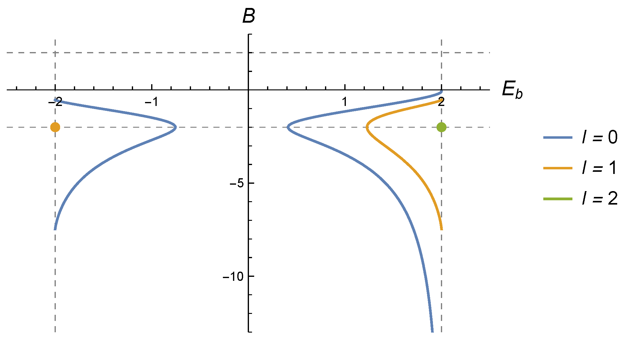
Figure 2.
The complex energy solutions of (71), corresponding to a singular pure scalar potential of intensity B concentrated on the circumference , are represented by points of different colors, for and , and various values of the intensity B in the interval . The blue curve represents the locus of the complex solutions to the imaginary part of (71), which does not depend on the strength B. The values correspond to an impenetrable wall at (with boundary conditions depending on the sign of B), and the corresponding real energy solutions are the admissible energies for an (anti)particle confined inside the circular box (except for the energy ), in the case , which corresponds to a bound state confined in the outer region). As B increases in absolute value the complex solutions shift towards the real axis, along the blue curve. The red points correspond to the critical value , at which absorption/emission of a bound state occurs at .
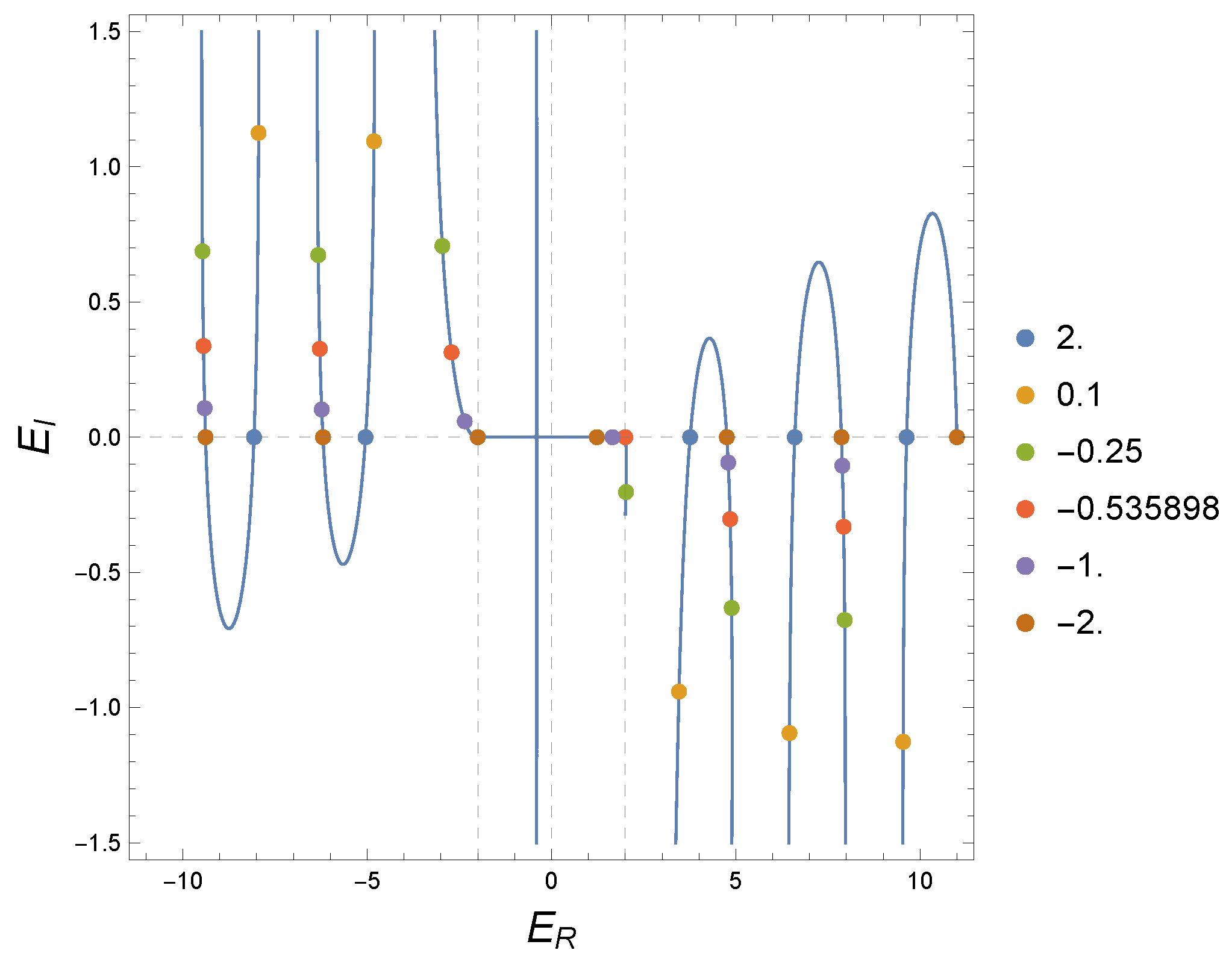
Figure 3.
The Wigner time delay (blue curves) for scattering states as a function of energy, for some values of the parameter B from (68) for a purely scalar strength (, arbitrary B), and for the same parameters as in Figure 2. The red points correspond to where are the complex energies that solve the equation (71). We note that the resonant energies approximate very well the sharp peaks (or valleys if ) of the Wigner time delay, and provide a scale for the Wigner time delay at the resonances.
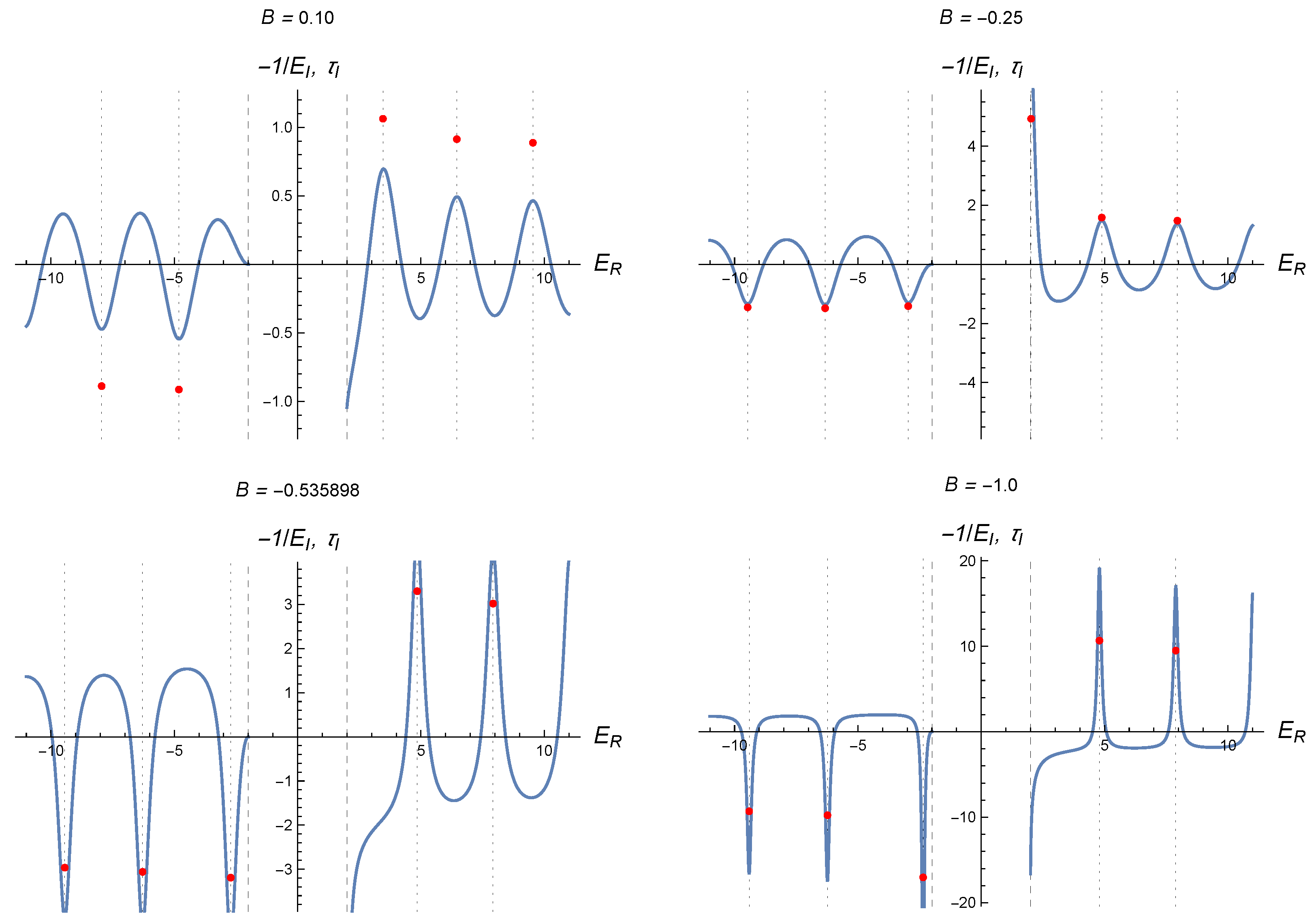
Figure 4.
Bound state energy as a function of the singular electric potential strength , for three values of the angular momentum l, with and . A single bound state will result if the curve crosses the horizontal line defined by the value of . This curve also shows the symmetry , as well as the relationships between the values of associated to critical and supercritical states discussed in the text.
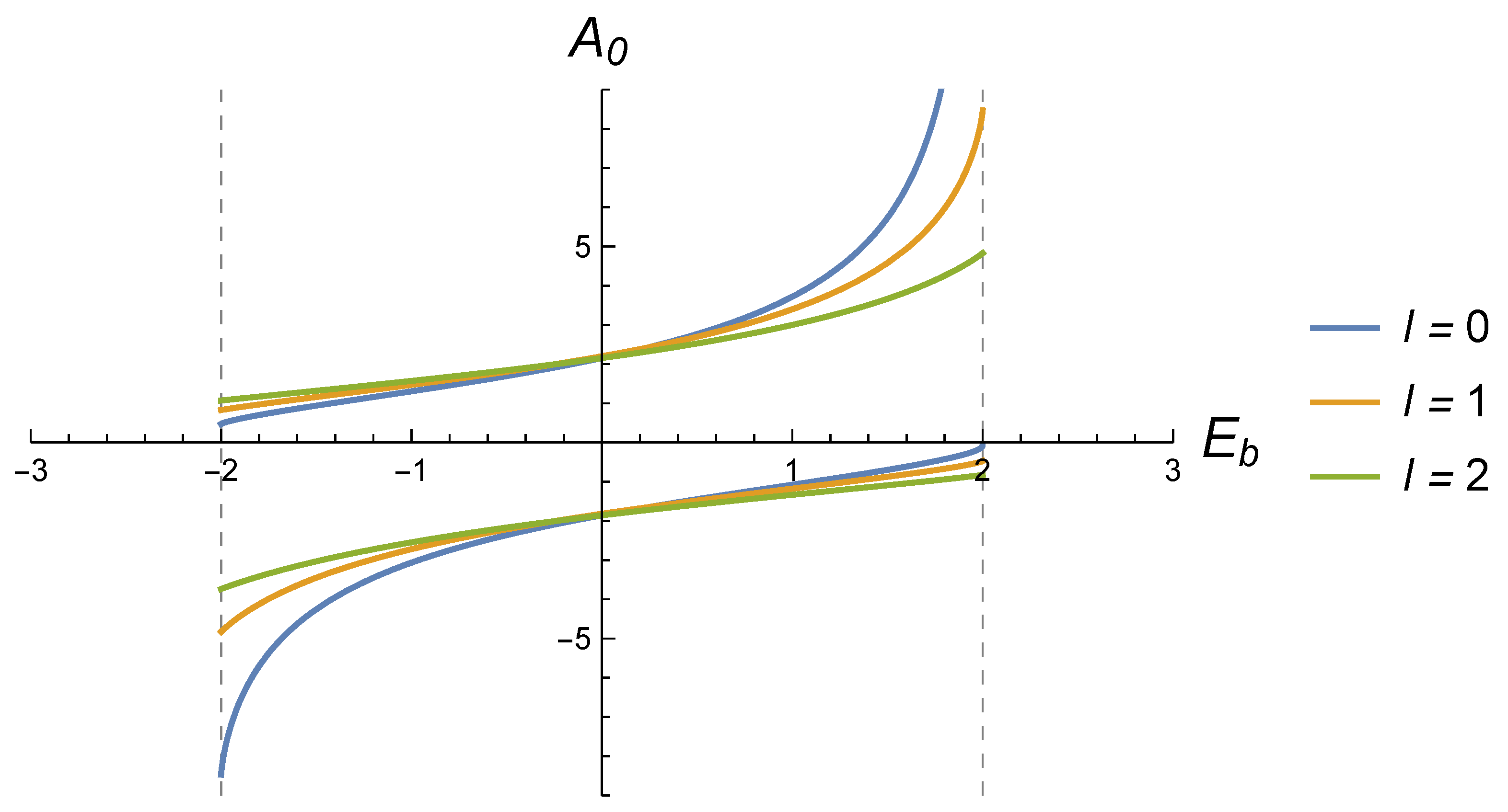
Figure 5.
The complex energies that are solutions of (76), corresponding to purely outgoing scattering states for a pure electrostatic potential (, ), are represented by points of different colors, taking , and . The blue curve corresponds to all solutions to the real part of (76), which do not depend on the value of . As the strength varies from 0 to ∞, the corresponding complex energies move from left to right along the blue curve. Due to the symmetry, the same happens as varies from to 0. With increasing values of , a bound (supercritical) state is captured at (green dot) and emitted at (brown dot).
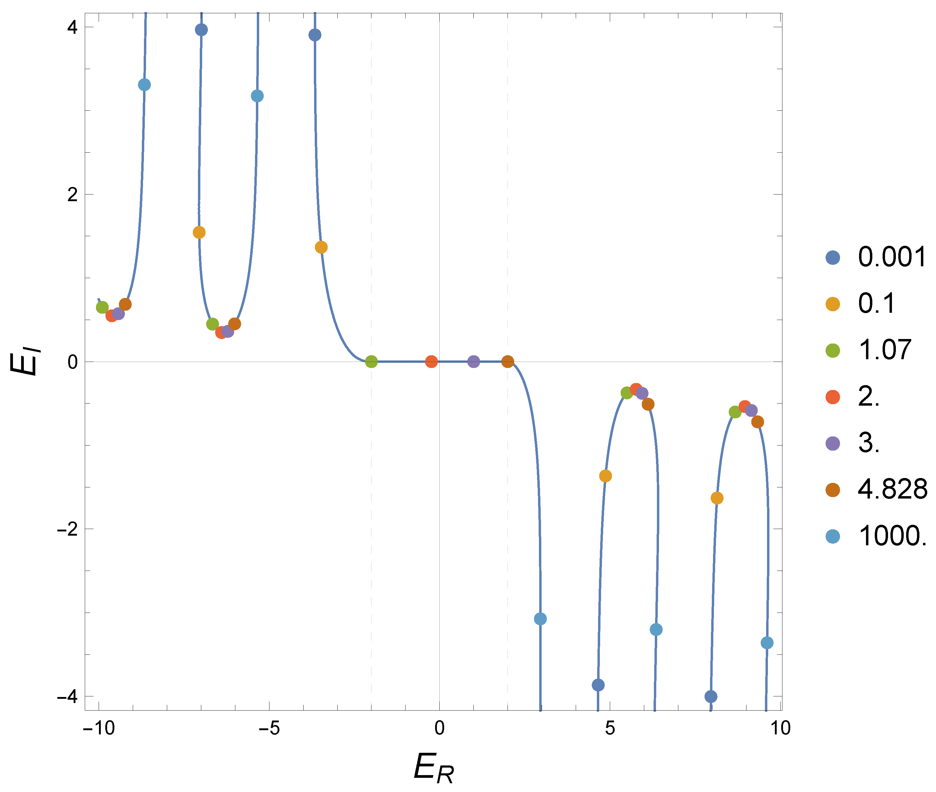
Figure 6.
The Wigner time delay (blue curves) for scattering states as a function of energy, for some values of the strength of a purely electrostatic shell at , for , and . The red points correspond to , where are the complex energies that solve the equation (76). We note that the resonant energies approximates very well the location of the sharp peaks (or valleys if ) of the Wigner time delay, and provides a scale for the Wigner time delay at the resonances.
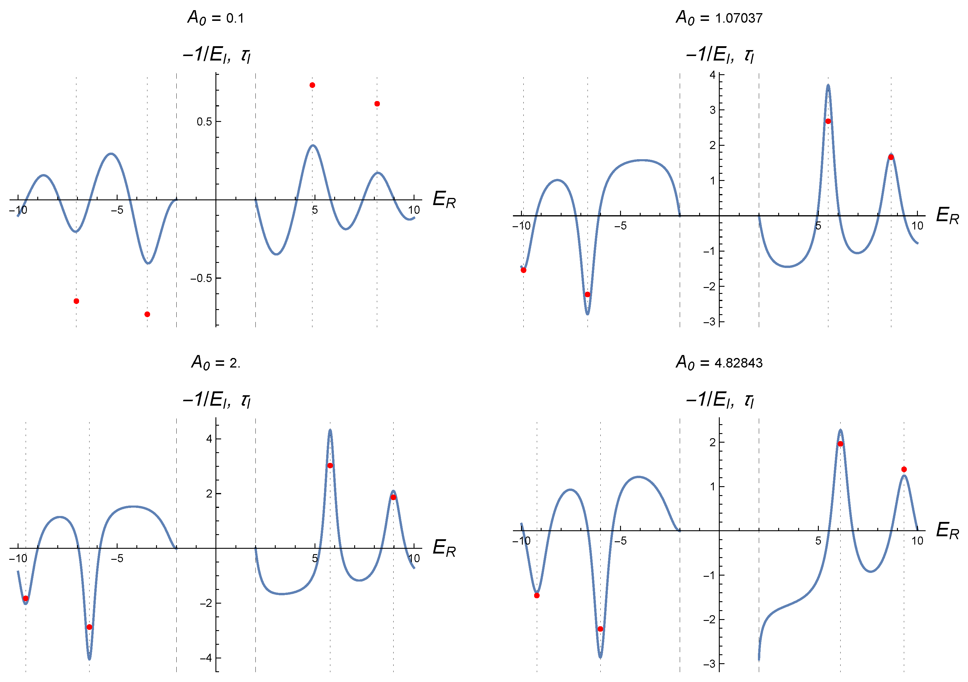
Figure 7.
Resonances in the complex plane for particles with mass and angular momentum as a function of the parameter a in (77) of a pure magnetic potential located at . The blue solid curve correspond to the locus of complex energies for which the imaginary part of the second equation in (78) vanishes, which does not depend on the value of a. The colored dots correspond to the values of complex energies that also satisfy the real part of that equation. As the parameter a grows from 0 to 1 (blue, yellow and green dots), the complex energy solutions move away from the real axis, and when a grows from 1 to (red and purple dots) they approach the real axis. The potential at turns into impenetrable walls when and (dark blue and violet points in the figure, respectively). In both cases the purely real complex solutions correspond to (anti)particles confined in the inner wall, and both cases show two remnant resonances with , which do not evolve to a confined state.
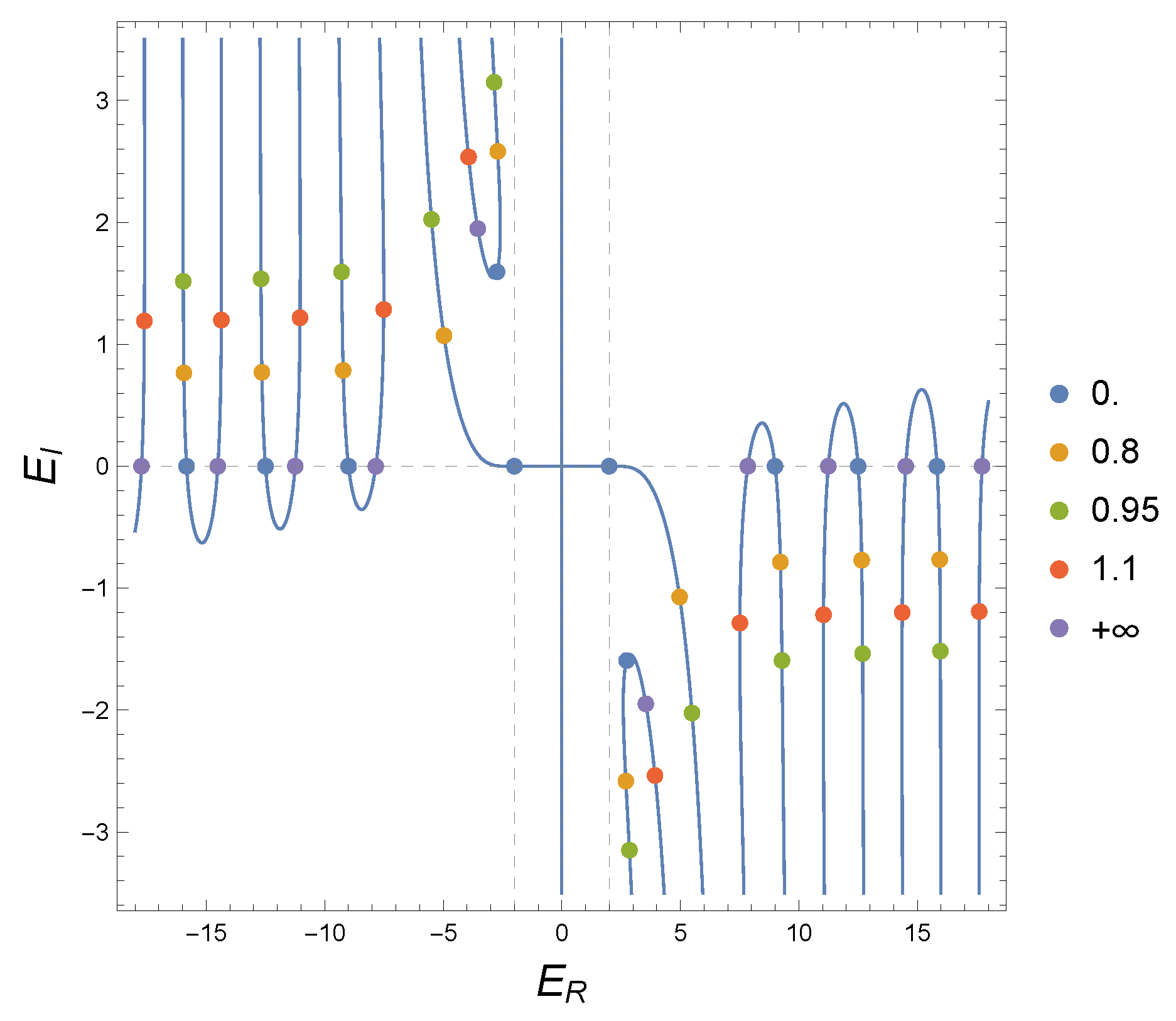
Figure 8.
The Wigner time delay (blue curves) for scattering states as a function of energy, for some values of the parameter a of (77) for a purely magnetic strength ( arbitrary), with , and . The red dots correspond to , where are the complex energies that solve the second equation in (78). We note that, for large values of , the real part of the resonant energies, , closely approximates the sharp peaks (or valleys if ) of the Wigner time delay, while provide a scale for the Wigner time delay at such resonances. For each value of a, there exist two complex resonances with that do not correspond to the locations of the Wigner time delay peaks: they are the points in the upper and lower regions of Figure 7 whose paths along the blue curve do not evolve towards the real energies of the admitted confined state in the limits .
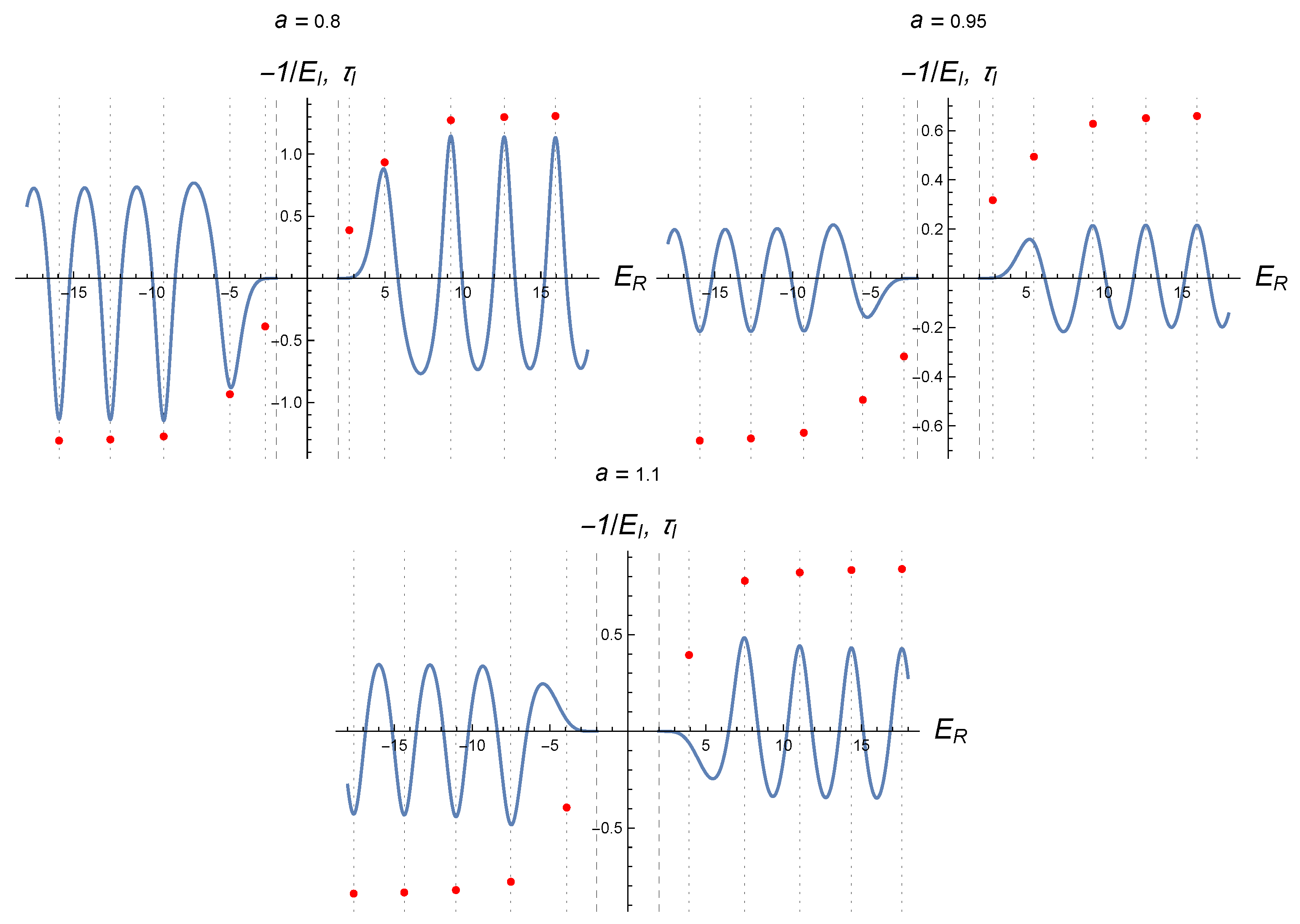
Figure 9.
Bound state energy for each value of the potential strengths , and for three values of the angular momentum l. In this plot and . For the system capture/emit a (quasi)bound state at when , respectively. Due to the absence of supercritical states for , in these case there are no emissions/capture of bound states at .
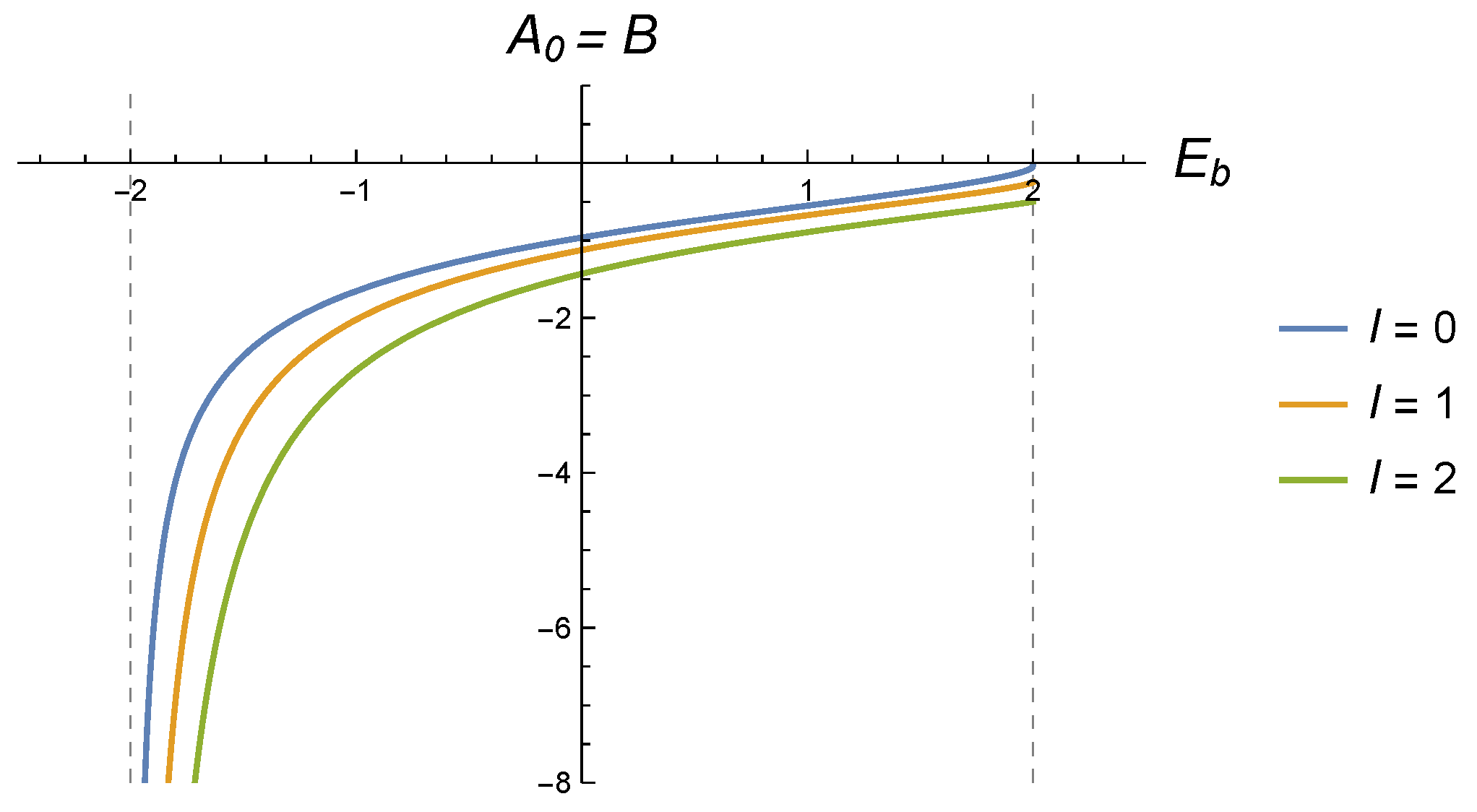
Figure 10.
Complex energies solving (80), corresponding to purely outgoing scattering states for a “delta shell" contact potential at (, ). In this plot, , and , and the energies are shown for several values of the potential strength (colored points). The vertical dashed lines correspond to . The real part of a complex energy corresponds to a resonant energy. In this graph, the solid blue lines correspond to the complex energies that solve the real part of (80), which does not depend on the value of the potential strength . When the potential strength crosses the value (red dots) the single bound state is emitted at (or absorbed, depending on the direction of the crossing). The dots on the real line in the region correspond to the bound state energies, while the dark blue point at corresponds to an antiparticle confined in the outer region of the impenetrable circle (). The other dots on the real line correspond to the discrete energies admissible for an (anti)particle confined in the inner region of an impenetrable circumference.
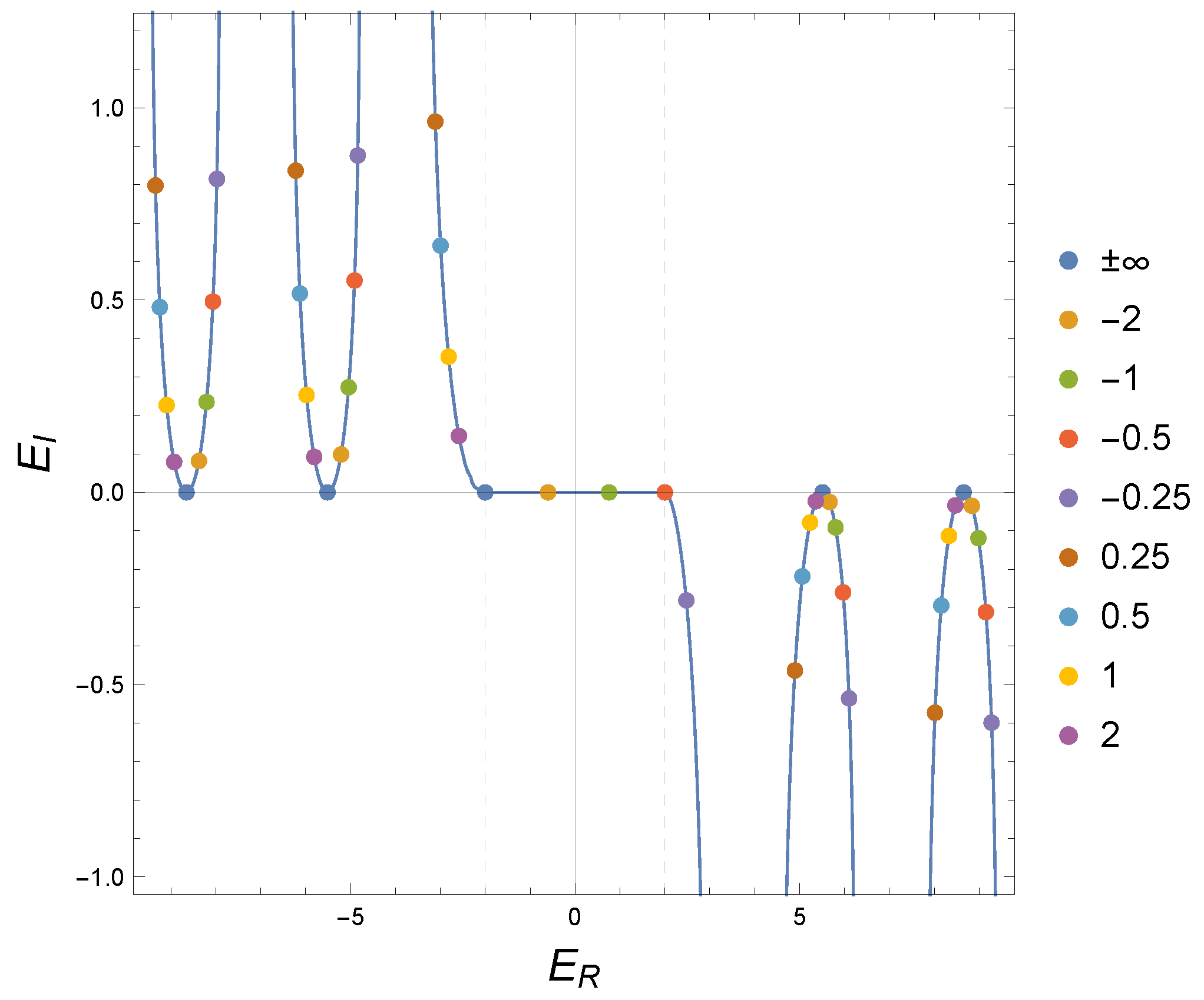
Figure 11.
The Wigner time delay (blue curves) for scattering states as a function of the energy, for some values of the potential strength of a delta shell contact potential at (, ), with , and . The red dots correspond to where are the complex energies that solve (80). The resonant energies closely approximate the sharp peaks (or valleys if ) of Wigner’s time delay, and provides a scale for Wigner’s time delay at the resonances.
Disclaimer/Publisher’s Note: The statements, opinions and data contained in all publications are solely those of the individual author(s) and contributor(s) and not of MDPI and/or the editor(s). MDPI and/or the editor(s) disclaim responsibility for any injury to people or property resulting from any ideas, methods, instructions or products referred to in the content. |
© 1996 by the authors. Licensee MDPI, Basel, Switzerland. This article is an open access article distributed under the terms and conditions of the Creative Commons Attribution (CC BY) license (https://creativecommons.org/licenses/by/4.0/).
Copyright: This open access article is published under a Creative Commons CC BY 4.0 license, which permit the free download, distribution, and reuse, provided that the author and preprint are cited in any reuse.


