
Submitted:
12 November 2025
Posted:
12 November 2025
You are already at the latest version
Abstract
A cascade deep-learning approach is proposed for optimizing the design and control of a dual-frequency induction heating system used in semiconductor manufacturing. The system is composed of two independent power inductors, fed at different frequencies, to achieve a homogeneous temperature profile along a graphite susceptor surface, crucial for enhancing layer quality and integrity. The optimization process considers both electrical (current magnitudes and frequencies) and geometrical parameters of the coils, which influence the power penetration and subsequent temperature distribution within the graphite disk. A two-step procedure based on Deep Neural Networks (DNNs) is employed. The first step, namely optimal design, identifies the optimal operating frequencies and geometrical parameters of the two coils. The second step, namely optimal control, determines the optimal current magnitudes. The DNNs are trained using a database generated through Finite Element (FE) analysis. The optimized system successfully achieved significant thermal uniformity across the susceptor surface, such that the temperature fluctuations over the entire disk radius were kept within ±7% of the target temperature (1100 °C). This significant improvement confirms the effectiveness of the deep learning-based cascade approach for solving high-dimensional Multiphysics inverse problems.
Keywords:
inverse problem
; multi-physics domain
; induction heating
; finite element analysis
; deep neural networks
1. Introduction
Accurate temperature control is one of the most important requirements in the semiconductor industry, especially in the epitaxial growth process of silicon layers. The quality of epitaxial layers is directly affected by temperature uniformity; in such a way that the thermal fluctuation can lead to structural defects, reduced surface quality and efficiency loss in semiconductor devices. Therefore, the development of heating methods with the ability to accurately control and high uniformity is a fundamental requirement in advanced semiconductor technologies [1,2].
One of the new and efficient methods in this field is induction heating. This method uses electromagnetic induction to convert electrical power into heat directly inside the conductive object. When time-varying current flows in an inductor, eddy currents are induced in conductive materials close to it and the temperature of those parts increases because of the joule losses [3,4]. The advantages of this method compared to traditional heating are very significant: higher energy efficiency (more than 90%), high response speed, no need for direct contact with the object, reduced pollution and greater controllability [5,6,7]. Induction heating system also has significant safety and environmental advantages due to the absence of an open flame and the absence of toxic by-products [8].
Despite these advantages, the design and control of induction heating systems is not an easy task. One of the main challenges is the precise adjustment of parameters such as position of the coils, frequency and current feeding the coils, since any incorrect choice can cause inhomogeneous heating and reduce the efficiency of the process. Furthermore, the complexity of the problem increases significantly when two independent frequency sources are used simultaneously, because the magnetic and thermal fields from each coil simultaneously involve the piece to heat [9].
For this reason, over the last two decades, numerical methods such as Finite Element Analysis (FEA) have replaced analytical models for accurate simulation of electromagnetic and thermal fields [10,11]. These methods allow for the investigation of physical details but are computationally expensive. Solving an electromagnetic and thermal coupled problem in time domain requires a long time and powerful hardware resources. This becomes a serious obstacle, especially in optimal design, which requires running thousands of simulations [12,13].
In the forward problem, given input parameters such as frequency and coil current, the temperature distribution is calculated. In practice, however, the problem is usually an inverse problem [9]: a target temperature profile is prescribed (e.g., uniform temperature across the susceptor surface) and the combination of electrical and geometric parameters generating this profile has to be determined [14].
Specifically, in our previous work [9], forward and inverse problems have been investigated using the electrical parameters (frequency and current amplitude of both coils) while the coil geometries were fixed. The main goal was to show the capability of surrogate models for predicting the temperature profile based on current magnitudes and frequency of both coils in forward problems and use the surrogate model in inverse problems. While here, by varying also the geometries of coils, the design space is much bigger and more complex.
The inverse problem is computationally and algorithmically much more complex to solve than the forward problem, because there is a nonlinear and coupled mapping between inputs and outputs. In addition, the presence of several variable parameters (frequency, current, coil geometries) makes the search space very large and difficult to solve.
For this reason, the use of innovative approaches to solve the inverse problem becomes necessary. In this study, a cascade approach based on deep learning is proposed, which has significant advantages compared to classical methods. This approach consists of two stages: in the first stage (optimal design), the frequencies and geometric parameters of the coils are chosen in such a way that the first step necessary for uniform heating are provided. In the second stage (optimal control), the values of the supply currents of each coil are determined so that the temperature distribution matches as possible to the target profile. This cascade structure reduces the complexity of the problem, because instead of solving one large and expensive problem, two simpler and more controllable problems are solved. Moreover, the use of deep neural networks in each stage allows an efficient and fast nonlinear mapping between parameters and temperature.
From a practical application perspective, the present study focuses on a dual-frequency induction heating device used in the epitaxy growth process, as described in two patents (Forzan, M.; Crippa, D.; Preti, S. Deposition Reactor with Inductors and Electromagnetic Shields 2021, EP3870734A1; Ogliari, V.; Forzan, M.; Preti, S. Inductively Heatable Susceptor and Epitaxial Deposition Reactor 2017, WO2017137872A1) and a study [15]. The device consists of a flat graphite susceptor with a certain thermal conductivity and specific resistance, which acts as a substrate in the deposition reactor [16]. To provide uniform heating, two copper coils are considered: an inner coil with a limited number of turns, which current operates in the higher frequency range, and an outer coil with a pancake structure, which is fed at lower frequencies. The combination of these two coils allows for a more precise control of the temperature distribution.
Overall, the aim of this research is to show that a cascade approach based on deep neural networks can be effectively applied to solve the inverse problem in dual-frequency induction heating systems while significantly reducing the need for heavy finite element calculations. In contrast to classical optimization-based methods, which require running thousands of costly simulations [17], the computational burden is significantly reduced in the present approach. Moreover, this method has an important advantage over single step learning models that approximate the entire complex mapping between input and output in one go: dividing the problem into two separate steps (design and control) simplifies the search space and improves the accuracy at each step.
The results of this research have direct application in the design and control of a new generation of epitaxy reactors and can provide a significant improvement in the quality of semiconductor layers.
2. The Field Model
2.1. The Device
The system under study is a benchmark dual-frequency induction heating system for silicon epitaxy growth applications as the case study [15]. The heating disk is a flat, circular graphite susceptor with a diameter of 500 mm. This susceptor acts as the workpiece in the deposition reactor and the aim is to achieve a uniform temperature distribution over its upper surface. To apply the inductive power, two independent copper coils are used: the inner coil (solenoid) with 7 turns and the outer coil (pancake) with 6 turns. The geometry of the device can change. Specifically, in addition to the electrical parameters (frequency and current magnitude of each coil), several geometric parameters of the coils are also considered as design variables. This allows to tune the penetration depth, shaping the power distribution, and finally improving temperature uniformity. These geometric parameters, which are the distance from gravity center of the grouped coils to the z = 0 line, denoted as x1 to x4 in the rest of the article (according to Figure 1), determine the shape of the coils and their relative distance to the susceptor: they are involved in the “optimal design” process. Thus, the design problem of this system is not limited to the choice of frequency and current magnitudes but is a simultaneous electrical-geometric problem that directly affects the thermal output. The two coils are fed independently: the inner coil with higher frequencies facilitates temperature control of the central region, and the outer coil with lower frequencies improves uniformity of the peripheral regions. These simultaneous degrees of freedom in both electrical (current/frequency values) and geometric (parameters x1 to x4) domains, are the basis of the optimization framework implemented through the deep learning-based cascade approach, presented in the following sections.
2.1. The Finite Element Model
The finite element model of the device is built axisymmetrically with respect to the z-axis in COMSOL Multiphysics 6.0 [18]. For the sake of generality an A-V formulation has been used to enforce the uniqueness of the field solution that would be mandatory in the case of a 3D analysis. Accordingly, magnetic analyses are solved in time-harmonics with the A-V formulation. The governing equations for magnetic vector potential () and electric scalar potential () are derived from Maxwell’s equations and the continuity equation from the electric field definition , respectively:
where is the complex vector of the current density, and are the material magnetic permeability and electrical conductivity, respectively, and the angular frequency relevant to the frequency f of the current. This coupled A-V system is made uniquely solvable by enforcing a Gauge condition on the magnetic potential, typically the Coulomb Gauge (), which is required to decouple and uniquely solve the system.
As mentioned before, the magnetic analysis is performed in time-harmonics and the fields are calculated separately for each frequency, resulting in a power density distribution, see Figure 2. Then, as the problem is a weakly coupled magneto-thermal problem, utilizing the superposition principle, the results for each coil are added together to obtain the distribution of the induced power density () in the graphite disk as a source for thermal model, see Figure 3. This method is particularly useful in dual-frequency problems, since directly performing a simultaneous simulation with two frequency sources would require solving a very complex and expensive multi-physics problem and it is not straightforward [19]. The superposition of the power density is:
where and are the power density of each coil, and by knowing , where is the magnetic field of the coil i, the condition to fulfill in order to properly applying the superposition of the two power densities is as follows:
where fi is the frequency of the coil i and mi is a positive integer number. This condition ensures that the two harmonic fields are synchronized with each other, and their superposition can be used validly in thermal analysis.
After calculating the power density, this value is entered into the heat equation as a heat source for equation 5:
where is the thermal conductivity. The thermal analysis is solved at steady state condition and handles both convective and radiative contributions for heat exchange at the boundaries. The leaving heat flux from the surface is described in Equation 6:
where is the Stefan-Boltzmann constant, is the external temperature, is the convective exchange coefficient and ε is the emissivity [20]. The terms and , represent the convective and radiative terms, respectively. Based on the literature [9,16] the considered values of the electrical, magnetic, and thermal material properties used in this study are reported in Table 1.
While the magnetic domain is composed of graphite disk, coils, ferrite ring and a surrounding air domain, the thermal domain is composed of the graphite disk and the handler, and the boundary conditions are applied to its boundaries.
The mesh of the magnetic model consists of over 19,000 second-order elements, with sensitive areas such as the disk, the disk boundary and the coils discretized with a mapped or finer mesh to improve the simulation accuracy, as shown in Figure 4. Typical magnetic field and temperature distributions of each coil contribution are shown in Figure 5 and Figure 6.
Finally, it should be emphasized that, in the present study, this finite element model is used only as a database generator and for the assessment of the results. In other words, hundreds of different cases with varying currents, frequencies, and coil geometric parameters (x1 to x4) are simulated and their results are used to train deep neural networks in a cascade approach. In this way, the finite element model plays the role of creating an accurate database for machine learning models, rather than being directly involved in the optimization process.
3. Cascade Approach
The optimization problem reads as follows: find a set of electrical and geometric parameters that produce a target temperature profile (e.g., uniform across the susceptor surface). Instead of solving a large, high-dimensional problem in one go, the present approach divides the problem into two separate phases to both reduce complexity and increase the stability and accuracy of the solution. As shown in Figure 7, these two phases are:
3.1. Phase 1: Optimal Design (OD)
In this step, the input to the deep neural network is the target temperature profile (a vector of 250 points on the reference line of the susceptor surface) and the output is the key geometric parameters and both frequencies, such that put the ground for creation of a uniform temperature profile are provided. The key point here is how to select the training data for the OD neural network. Since the inner coil has the greatest impact on the central part of the susceptor, the initial database is filtered by a specific physical criterion: only samples are selected that, in the first 25 mm of the disk radius, have a temperature within ±12.5% of the target temperature (1100 °C). This ensures that in all data used for OD, the inner coil has played its role in heating the central region correctly.
Accordingly, the inner coil frequency f1 can be obtained statistically (mean on the filtered database) and does not need to be predicted directly by the neural network. This choice simplifies the design problem, and the OD neural network focuses only on the mapping between the temperature profile and x1, … x4, f2. At the same time, it is guaranteed that the inner coil works properly in the central region.
In this way, OD operates more accurately: the geometry and frequency of the outer coil are optimized, while the inner coil frequency is extracted statistically from valid data. This structure both reduces the complexity of the problem and ensures the stability of the results.
3.1. Phase 2: Optimal Control (OC)
After fixing the geometry and frequencies, a second deep neural network learns the mapping of the target temperature profile into the amplitude of the two-coil currents using a new database. Hence, geometric parameters and frequencies are known, given the temperature profile as input, the output will be I1, I2. At this step, the field and induced power patterns are somehow determined, and the role of the network is to calibrate the power intensity to accurately reach the target temperature. Thus, instead of searching simultaneously in the complex space of x1…x4, f1, f2, I1, I2, the geometric-frequency subspace is first determined and then the intensities of the currents are identified. This is the advantage of scaling and dimensionality reduction in the cascade approach, which is more stable and interpretable than single-stage learning.
4. Database
To effectively train the networks and avoid the computational burden of direct FEA-based optimization, two separate databases are needed (see Figure 7). To ensure efficient coverage of the input space for generating the training dataset, the Latin Hypercube Sampling (LHS) technique was employed. In this method, the cumulative probability range [0,1] of each variable is divided into n equiprobable intervals [21]:
A random value is then selected and mapped through the inverse cumulative distribution function , yielding:
where denotes the cumulative distribution function (CDF) of the variable, defined as:
where is its probability density function (PDF). Thus maps a uniform distributed random number to a sample value that follows the target probability distribution specified by .
For a d-dimensional problem, this procedure is repeated for each variable independently, and the resulting samples are combined using random permutations across dimensions. This produces a matrix of size , where each column approximates the target marginal distribution, while collectively ensuring a more uniform coverage of the multidimensional input space.
The main advantage of LHS compared to simple random sampling is that it guarantees that all portions of each input distribution are represented, thereby reducing sampling bias and improving the statistical representativeness of the generated dataset [22,23].
Using Latin Hypercube sampling on the input parameters (currents, frequencies and geometric parameters (x1…x4)), 2,500 FE simulations are run. The ranges of each parameter have been reported in Table 2.
The output of each simulation is a 250-point temperature profile on the susceptor surface reference line. As previously mentioned, in the OD phase, the data are filtered based on the criterion of inner coil contribution to the central region: samples are held such that in the first 25 mm of radius, the temperature is within ±12.5% of 1,100°C. This ensures that the chosen geometry/frequencies actually provide heating of the core. For the OC phase, by keeping constant the frequencies and geometric parameters of the OD phase, and varying the currents (I1, I2) in their working intervals, 400 FE analyses are performed to sample the effect of only the currents on the temperature profile, so new database will be prepared called DB 2. In both cases, 80% of databases were used for training, 10% for validation and 10% for testing.
5. Results
In this study, the optimization process is carried out in two consecutive stages: optimal design (OD) and optimal control (OC). For each stage, an independent deep neural network (DNN) is designed and trained to model the inverse relationship between the target temperature profile and the relevant geometric and electric parameters. To evaluate the accuracy of the inverse surrogate models, three statistical indices are used.
Mean Absolute Percentage Error (MAPE)
where is the vector of true values calculated with FE model, and is the vector of values predicted by relevant surrogate model. and are 250 temperature values along the susceptor surface and the number of observations, respectively.
Root Mean Square Error (RMSE)
Coefficient of Determination ()
where is the mean value of the jth temperature profile.
5.1. DNN for Optimal Design (DNNOD)
In the optimal design step, the goal was to predict the coil geometric parameters x1…x4 and the outer coil frequency f2 based on the target temperature profile. The input data to the network consists of temperature profiles at 250 points on the susceptor surface, and the output consists of five design parameters x1…x4 and f2. After training the network on the design database (DB1), which consisted of 1947 filtered observations from finite element simulations. The structural details of deep neural network (DNN) designed for this step and the assessment results are reported in Table 3 and Table 4, respectively.
The optimizer is Levenberg–Marquardt and the activation function Tan-sigmoid (hyperbolic tangent sigmoid) was chosen because it introduces nonlinearity, allows outputs between −1 and 1 for faster and balanced learning [24,25], and works efficiently with the Levenberg–Marquardt optimizer in regression tasks. All DNNs in this study, trained in Matlab 2024b [26].
The mean absolute percentage error (MAPE) value for the test set was 17.9% with 94.8% accuracy. This value is considered to be good and reasonable accuracy considering the nonlinear and multi-response nature of the inverse problem and indicates that the model is able to accurately reproduce the overall trend of changes in the geometric parameters and frequency of the outer coil. Prediction Vs. actual value is also presented in Figure 8, which shows that the model predictions followed the bisector.
Table 5 shows the results of OD phase for the ideal temperature profile, which is 1,100˚C along the susceptor surface.
5.2. DNN for Optimal Control (DNNOC)
In the optimal control step, assuming the geometric parameters and frequencies to be constant (the result of the OD step), the goal was to predict the current magnitudes of the two coils in such a way that the target temperature profile is obtained with high accuracy. For this purpose, a deep neural network was designed and trained with a second database (DB2). The network structural details and assessments are reported in Table 6 and Table 7, respectively.
After evaluation of the OC model, MAPE values were obtained on all data sets are less than 0.01%, indicating a very high accuracy in predicting the optimal current magnitudes, which is also shown in Figure 9 (predicted vs. actual for OC phase). Table 8 shows the results of OC phase for the ideal temperature profile.
Figure 10 and Figure 11 show the results obtained by applying the proposed cascade approach. In Figure 10, a comparison between the initial geometry of the system and the optimized geometry obtained by OD phase of the cascade approach is presented. It can be seen that after applying the proposed method, the geometric structure of the system has changed and the distribution of the coils and their relative positions have been modified in a way that creates a better balance in the magnetic field distribution.
Figure 11 also shows the temperature profiles obtained from both geometries in comparison with the target profile. As can be seen, the initial temperature profile (red curve) has a significant distance from the target value and the central and peripheral areas of the susceptor have a wide thermal fluctuation. In the OD stage, which involves determining the geometric and frequency parameters, the temperature distribution is closer to the target value (purple curve), but a slight non-uniformity is still observed, while the feed currents are kept similar to the initial values and their fine-tuning is performed in the next stage, OC. Finally, by performing the OC stage and adjusting the coil feed currents, the optimized temperature profile (black curve) is almost completely within the ±7% tolerance around the target value (1100°C) and is in good agreement with the target profile (blue dashed line).
These results indicate a clear improvement in the temperature distribution and the modification of the system geometry after applying the proposed approach. A more detailed analysis of these results is provided in the Discussion section.
6. Discussion
The results obtained from the proposed cascade approach show that separating the process into two distinct stages (design and control) in combination with deep learning-based modeling significantly reduces the complexity of the mapping between design parameters and temperature profiles. In fact, solving the problem in two separate phases causes each neural network to cover only a part of the design space, thus reducing the dimensions of the search space and nonlinear relationships at each stage and making the network training more stable and faster.
In the design optimization phase, geometric and frequency variables are considered with a smaller dimension than in the single-stage solution; this directly affects the prediction accuracy, since the geometric parameters determine the field distribution and the pattern of induced currents, which can be expected to have a significant impact on the thermal behavior of the system. In the control phase, the network only deals with currents, which have a simpler and more approximated mapping than the entire combination space. This reduction in complexity at each stage allows neural networks to approximate nonlinear mappings with greater stability and faster convergence, which naturally leads to improved accuracy and increased computational efficiency of the entire process.
In the optimal design (OD) stage, the surrogate model was able to model the nonlinear relationship between geometric parameters, frequencies and temperature distribution with reasonable accuracy (MAPE ≈ 17.9%). The results showed that the inner coil frequency in the average range of about 60 kHz has an optimal value and is responsible for the main contribution to the heating of the central area of the susceptor. In contrast, the outer coil frequency is about 5 kHz, which plays a key role in temperature uniformity in the peripheral area. This separation of the two coils has caused the resulting induction field to have a more balanced power distribution and a more suitable penetration depth than the initial geometry.
In the optimal control (OC) stage, with the geometry and frequencies fixed, the second neural network was able to predict the optimal currents with very high accuracy (MAPE < 0.01%). The results of this model show that reducing the current of both coils compared to the initial value not only saved energy but also increased thermal uniformity. This improvement was due to the fine-tuning of the current amplitude, which caused the induced current lines to be distributed in the center and periphery with a better balance.
Figure 10 and Figure 11 clearly confirm this point: in the initial geometry, the temperature of the peripheral regions exceeded 1200°C and the central region remained cooler, while after optimization, the temperature profile over the entire disk radius was within ±7% of the target value (1100°C).
From a physical perspective, this improvement is due to four main factors:
1- simultaneous optimization of geometry and electrical parameters, which has allowed for optimal adjustment of the field penetration depth in each region;
2- a two-stage cascade structure that has reduced the search space and prevented instability in the inverse mapping;
3- the use of deep neural networks that are able to reproduce nonlinear and multivariate mappings between physical parameters and thermal response with high accuracy;
4- More precise and targeted selection of geometric parameters can play an effective role in increasing the accuracy of inverse models, because geometry directly controls the magnetic field distribution and induced power pattern. Consequently, if these geometric parameters are redefined or improved to achieve higher accuracy, these changes can be applied at the Optimal Design stage, which is simpler and more stable in terms of structure compared to one stage solving, so that the learning network in the control stage is not affected by the increase in complexity and the overall stability of the approach is maintained.
Overall, the results of this study show that the proposed approach, by separating the process into two separate stages and using surrogate models based on deep learning, can be an efficient alternative to classical methods based on direct optimization. In the previous study [9], with has only four dimensions search space, the NSGA-II method with the leading surrogate model required a significant time for training and then performing a large number of analyses to solve the inverse problem to achieve appropriate accuracy. While in the present problem, due to the increase in the dimensions of the variable space and the simultaneous dependence of geometric and electrical parameters, the use of the same classical approach will require much more computational time.
On the other hand, in the same previous study [9], it was shown that the cascade structure has much higher accuracy than the direct optimization method even in the four-dimensional search space. Therefore, considering the higher dimensions and greater complexity in the present problem, the proposed cascade approach is also expected to provide more accurate and efficient performance. This method can facilitate the development path of new generation epitaxy reactors that require very high thermal accuracy.
7. Conclusions
In this study, a novel approach based on Cascade Deep Learning was performed to solve the inverse problem in the design and control of a dual-frequency induction heating system. By dividing the overall process into two distinct steps—optimal design (OD) and optimal control (OC)—this approach was able to reduce the numerical complexity for each stage which cause significantly increasing the accuracy and stability of the predictions.
In the design phase, the surrogate model was able to reconstruct the relationship between geometric parameters, frequency, and temperature profile with acceptable accuracy and determine the optimal geometry and operating frequencies. In the control phase, the second network identified the feed currents that reproduced the target temperature profile with an error of less than 0.01%, indicating the very high capability of the method in accurately predicting the source of the thermal behavior of the system.
The final results obtained from applying the cascade approach produced remarkable thermal uniformity on the susceptor surface. In such a way, the temperature fluctuations in the entire disk radius were within ±7% around the target value (1,100°C). This improvement will not only increase the quality of epitaxial layers in semiconductor processes but also saves power consumption and increases the system lifetime.
From a scientific perspective, this research showed that combining deep learning methods with finite element modeling can be an effective and low-cost alternative to classical multi-physics optimizations. In particular, the separation of the design step from the control step resulted in greater stability of the networks, better interpretability of the results, and a significant reduction in the number of simulations required as discussed before.
Finally, it can be said that the presented approach can be generalized not only in the field of induction heating, but also in other multi-source or multi-physics systems and can provide a basis for the development of intelligent models in the design of next-generation reactors and similar industrial applications.
Author Contributions
Conceptualization, P.D.B., F.D. and M.F.; methodology, P.D.B, F.D. and M.E.M.; software, A.G., E.S. and M.E.M.; validation, M.F. and E.S.; formal analysis, P.D.B. and F.D.; investigation, A.G., E.S. and M.F.; resources, F.D.; data curation, A.G., E.S. and M.E.M.; writing—original draft preparation, A.G.; writing—review and editing, P.D.B., M.E.M., M.F.
Funding
This research received no external funding.
Data Availability Statement
Dataset available on request from the authors.
Conflicts of Interest
The authors declare no conflicts of interest.
References
- Deng, S.; Wang, Y.; Cheng, J.; Shen, W.; Mei, D. Measurement of Thermal Field Temperature Distribution Inside Reaction Chamber for Epitaxial Growth of Silicon Carbide Layer. ASME. J. Manuf. Sci. Eng. 2024, 146(7), 070901. [Google Scholar] [CrossRef]
- Baake, E.; Nacke, B. Efficient Heating by Electromagnetic Sources in Metallurgical Processes: Recent Applications and Develop ment Trends. Przegl ˛ad Elektrotech. 2010, 86, 11–14. [Google Scholar]
- Rudnev, V.; Loveless, D.; Cook, R. Handbook of Induction Heating. In Manufacturing Engineering and Materials Processing, 2nd ed.; CRCPress: Boca Raton, FL, USA, 2017; ISBN 978-1-4665-5395-8. [Google Scholar]
- Rudnev, V.; Totten, G.E. Induction Heating of Selective Regions. In Induction Heating and Heat Treatment; ASM International: Materials Park, OH, USA, 2014; pp. 346–358. ISBN 978-1-62708-167-2. [Google Scholar]
- Rapoport, E.; Pleshivtseva, Y. Optimal Control of Induction Heating Processes; Mechanical Engineering; CRC/Taylor & Francis: Boca Raton, FL, USA, 2007; ISBN 978-0-8493-3754-3. [Google Scholar]
- Fisk, M. Induction Heating. In Encyclopedia of Thermal Stresses; Hetnarski, R.B., Ed.; Springer: Dordrecht, The Netherlands, 2014; pp. 2419–2426. ISBN 978-94-007-2738-0. [Google Scholar]
- Di Barba, P.; Dughiero, F.; Lupi, S.; Savini, A. Optimal Shape Design of Devices and Systemsfor Induction-Heating: Methodologies and Applications. COMPEL Int. J. Comput. Math. Electr. Electron. Eng. 2003, 22, 111–122. [CrossRef]
- Vishnuram, P.; Ramachandiran, G.; Sudhakar Babu, T.; Nastasi, B. Induction Heating in Domestic Cooking and Industrial Melting Applications: A Systematic Review on Modelling, Converter Topologies and Control Schemes. Energies 2021, 14, 6634. [Google Scholar] [CrossRef]
- Di Barba, P.; Ghafoorinejad, A.; Mognaschi, M.E.; Dughiero, F.; Forzan, M.; Sieni, E. Optimal Multi-Physics Synthesis of a Dual-Frequency Power Inductor Using Deep Neural Networks and Gaussian Process Regression. Algorithms 2025, 18, 10. [Google Scholar] [CrossRef]
- Brazhnik, D.S.; Bolotin, K.E. Different Approaches to Taking Joule Heat into Induction Heating of Graphite Crucible. In Proceedings of the 2020 IEEE Conference of Russian Young Researchers in Electrical and Electronic Engineering (EIConRus), St. Petersburg and Moscow, Russia, 27–30 January 2020; pp. 616–618. [Google Scholar]
- Mannanov, E.; Galunin, S. Numerical Simulation of the Induction Heating Process of a Disk Profile. IOP Conf. Ser. Mater. Sci. Eng. 2019, 643, 012065. [Google Scholar] [CrossRef]
- Fisk, M.; Ristinmaa, M.; Hultkrantz, A.; Lindgren, L.-E. Coupled Electromagnetic-Thermal Solution Strategy for Induction Heating of Ferromagnetic Materials. Appl. Math. Model. 2022, 111, 818–835. [Google Scholar] [CrossRef]
- Jankowski, T.A.; Pawley, N.H.; Gonzales, L.M.; Ross, C.A.; Jurney, J.D. Approximate Analytical Solution for Induction Heating of Solid Cylinders. Appl. Math. Model. 2016, 40, 2770–2782. [Google Scholar] [CrossRef]
- Di Barba, P.; Mognaschi, M.E.; Cavazzini, A.M.; Ciofani, M.; Dughiero, F.; Forzan, M.; Lazzarin, M.; Marconi, A.; Lowther, D.A.; Sykulski, J.K. A Numerical Twin Model for the Coupled Field Analysis of TEAM Workshop Problem 36. IEEE Trans. Magn. 2023, 59, 1–4. [Google Scholar] [CrossRef]
- Forzan, M.; Maccalli, G.; Valente, G.; Crippa, D. Design of an Innovative Heating Process System for the Epitaxial Growth of Silicon Carbide Layers Wafer. In Proceedings of the MMP-Modelling for Material Processing, Riga, Latvia, 8–9 June 2006. [Google Scholar]
- Di Barba, P.; Dughiero, F.; Forzan, M.; Mognaschi, M.E.; Sieni, E. New Solutions to a Multi-Objective Benchmark Problem of Induction Heating: An Application of Computational Biogeography and Evolutionary Algorithms. Arch. Electr. Eng. 2018, 67, 139–149. [Google Scholar] [CrossRef] [PubMed]
- Koziel, S.; Ciaurri, D.E.; Leifsson, L. Surrogate-Based Methods. In Computational Optimization, Methods and Algorithms; Koziel, S., Yang, X.S., Eds.; Springer: Berlin, Heidelberg, 2011; Volume 356, pp. 49–75. [Google Scholar] [CrossRef]
- COMSOL. MultiphysicsSoftware for Optimizing Designs. Available online: https://www.comsol.com/ (accessed on 13 October 2025).
- Hömberg, D.; Liu, Q.; Montalvo-Urquizo, J.; Nadolski, D.; Petzold, T.; Schmidt, A.; Schulz, A. Simulation of Multi-Frequency Induction-Hardening Including Phase Transitions and Mechanical Effects. Finite Elem. Anal. Des. 2016, 121, 86–100. [CrossRef]
- Bay, F.; Labbé, V.; Favennec, Y.; Chenot, J.L. A numerical model for induction heating processes coupling electromagnetism and thermomechanics. Int. J. Numer. Methods Eng. 2003, 58, 839–867. [Google Scholar] [CrossRef]
- Shields, M.D.; Zhang, J. The generalization of Latin hypercube sampling. Reliab. Eng. Syst. Saf. 2016, 148, 96–108. [Google Scholar] [CrossRef]
- McKay, M.D.; Beckman, R.J.; Conover, W.J. A Comparison of Three Methods for Selecting Values of Input Variables in the Analysis of Output from a Computer Code. Technometrics 1979, 21, 239–245. [Google Scholar] [PubMed]
- Helton, J.C.; Davis, F.J. Latin hypercube sampling and the propagation of uncertainty in analyses of complex systems. Reliab. Eng. Syst. Saf. 2003, 81, 23–69. [Google Scholar] [CrossRef]
- Jagtap, A.D.; Karniadakis, G.E. How important are activation functions in regression and classification? A survey, performance comparison, and future directions. J. Mach. Learn. Model. Comput. 2023, 4, 1. [Google Scholar] [CrossRef]
- Hagan, M.T.; Demuth, H.B.; Beale, M.H.; De Jesús, O. Practical Training Issues. In Neural Network Design, 2nd ed.; (Self-Published): Stillwater, OK, USA, 2014; pp. 22–8–22–9. [Google Scholar]
- Train neural network. Available online: https://www.mathworks.com/help/deeplearning/ref/network.train.html, (accessed on 24 October 2025).
Figure 1.
Model of the device with design variables.
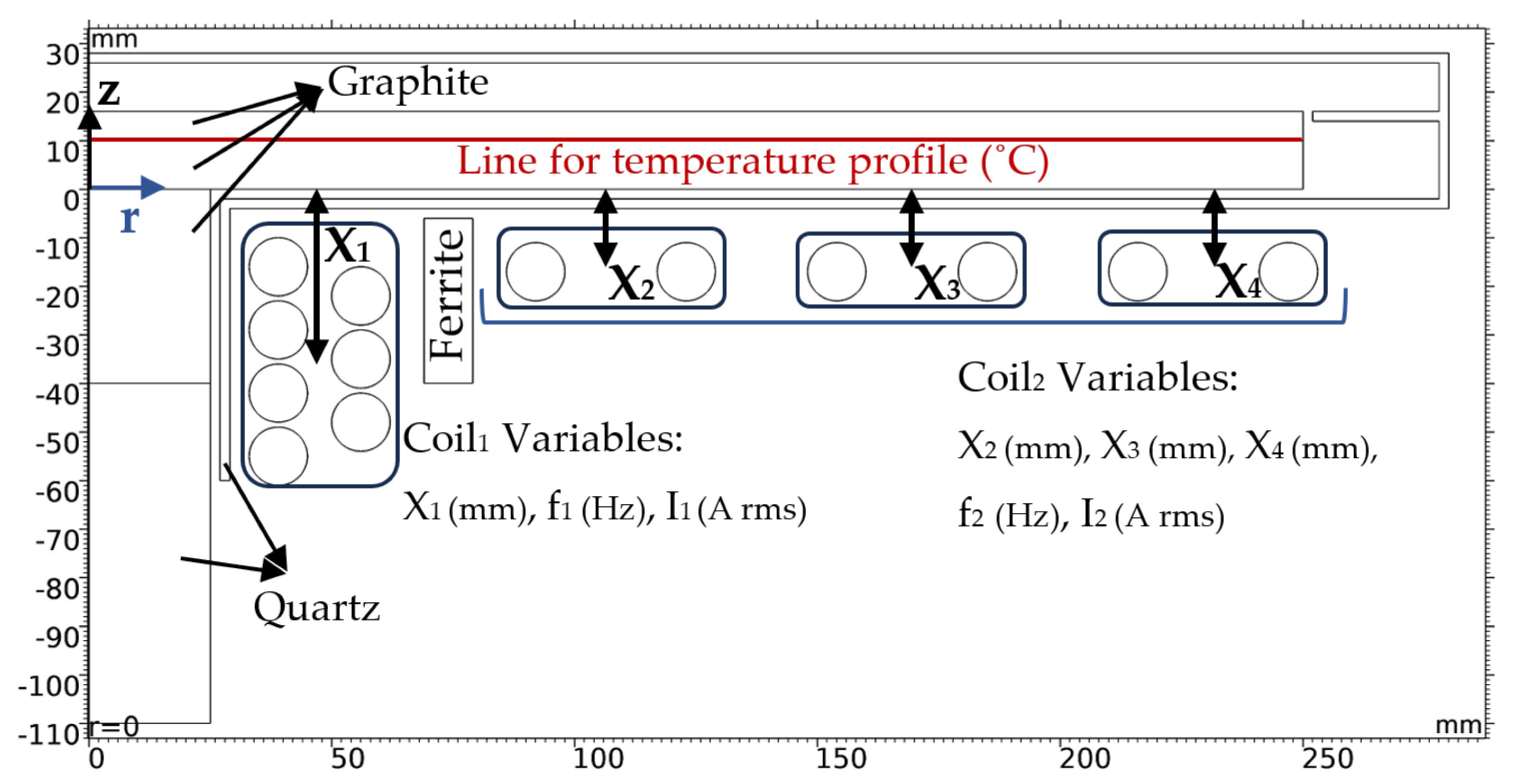
Figure 2.
Input/ output model of magnetic analysis.
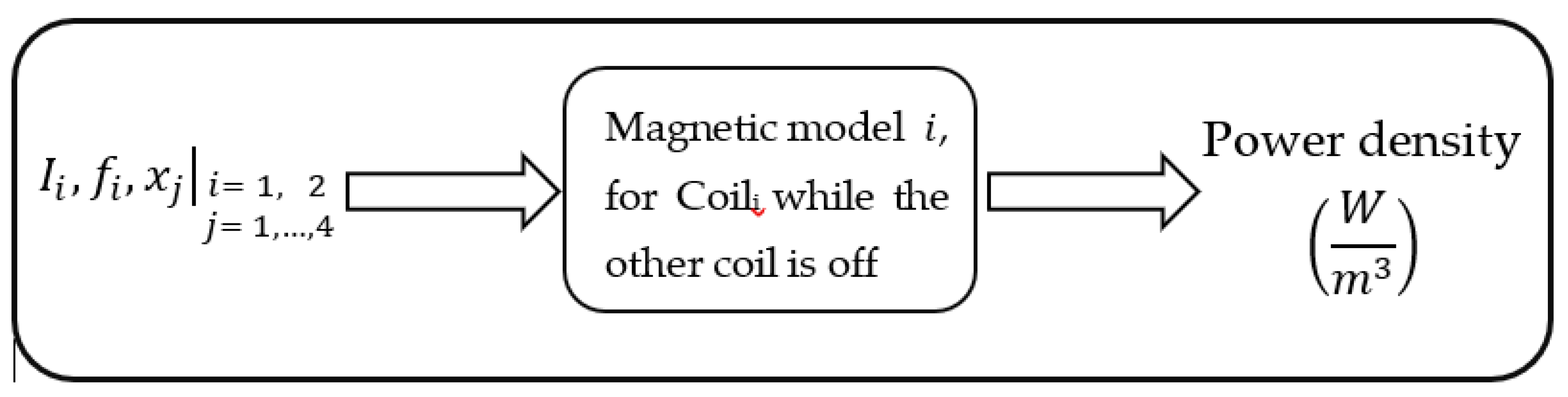
Figure 3.
Structure of combining magnetic and thermal model.
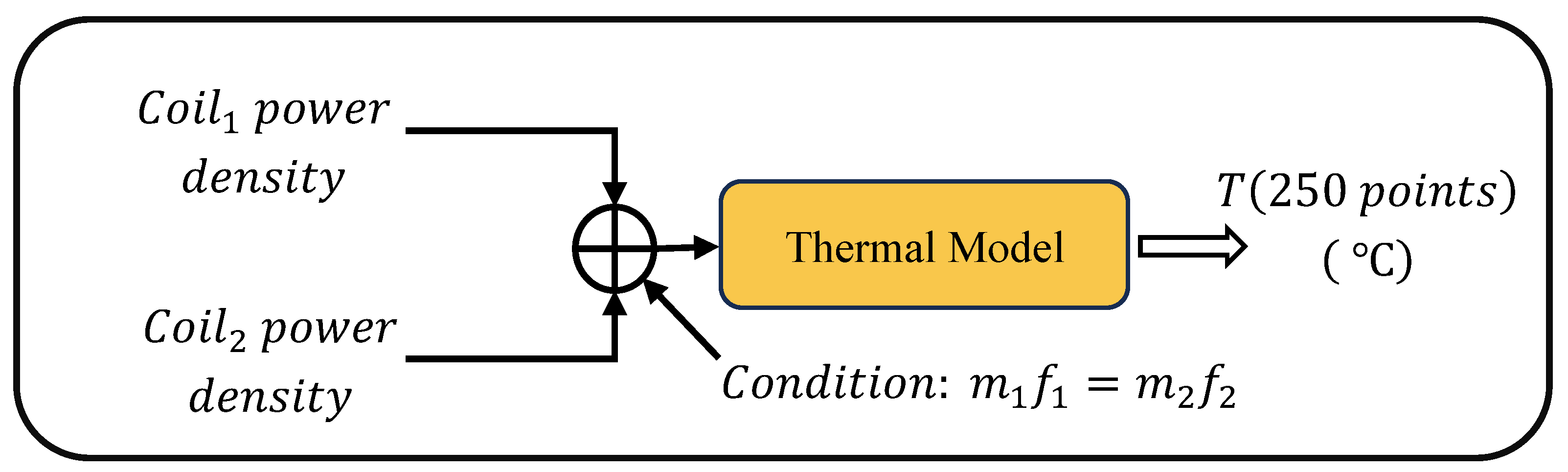
Figure 4.
Mesh details of the model.
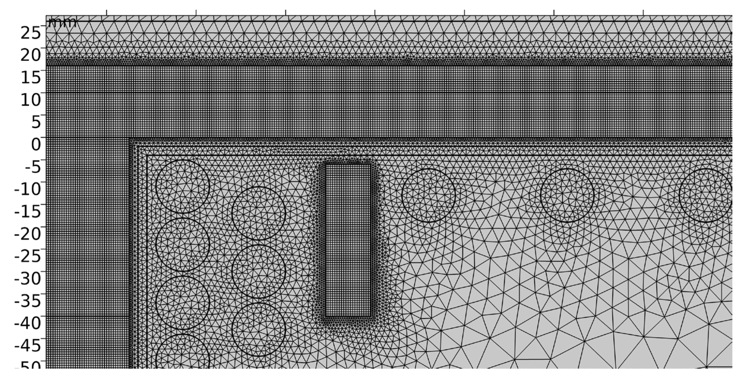
Figure 5.
Magnetic field (T) for a given configuration of the system: (a) First coil; (b) Second coil.
Figure 5.
Magnetic field (T) for a given configuration of the system: (a) First coil; (b) Second coil.
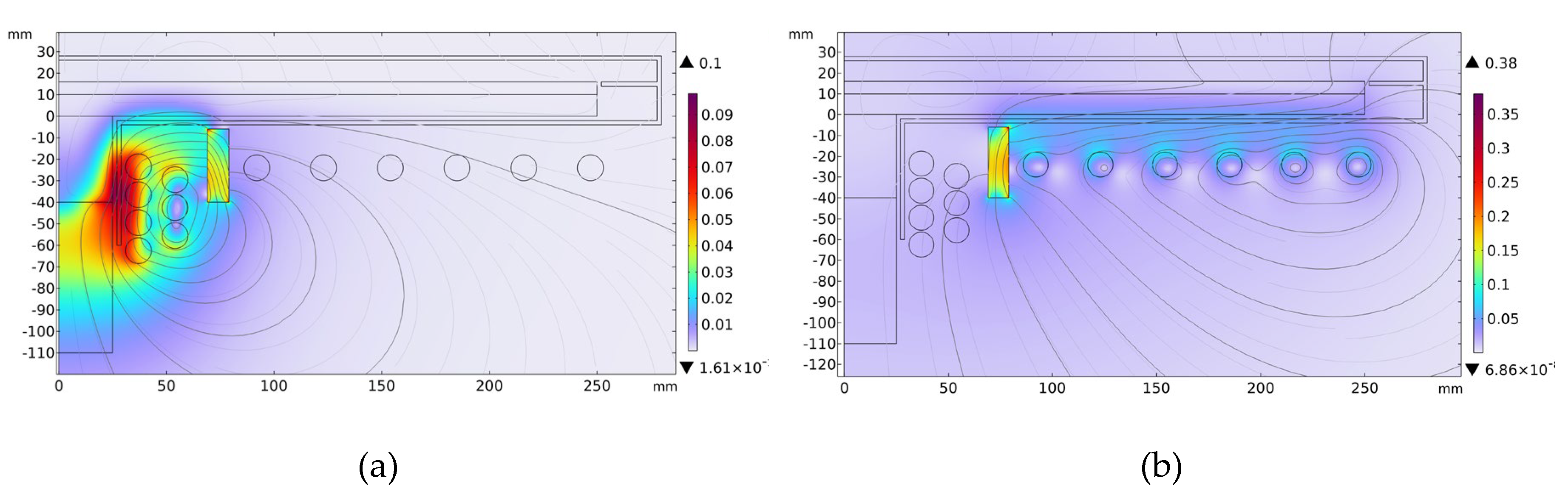
Figure 6.
Thermal map (˚C) for a given configuration of the system: (a) Temperature map results of first coil; (b) Temperature map results of second coil; (c) Temperature map influenced by the power density of both coils; (d) 3D view of the device temperature map.
Figure 6.
Thermal map (˚C) for a given configuration of the system: (a) Temperature map results of first coil; (b) Temperature map results of second coil; (c) Temperature map influenced by the power density of both coils; (d) 3D view of the device temperature map.
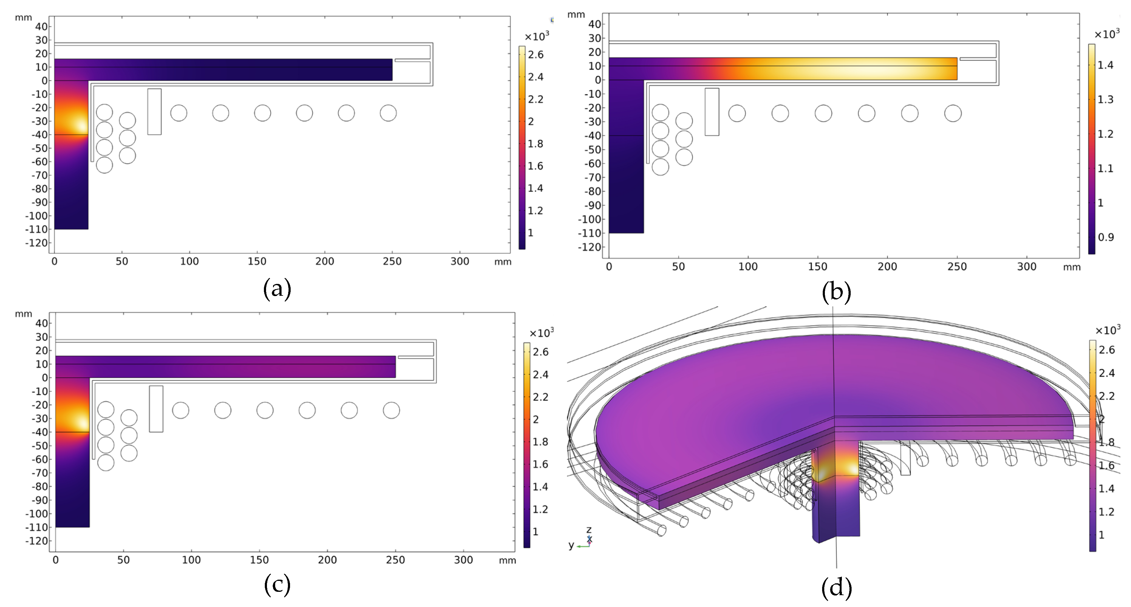
Figure 7.
Cascade approach flowchart.
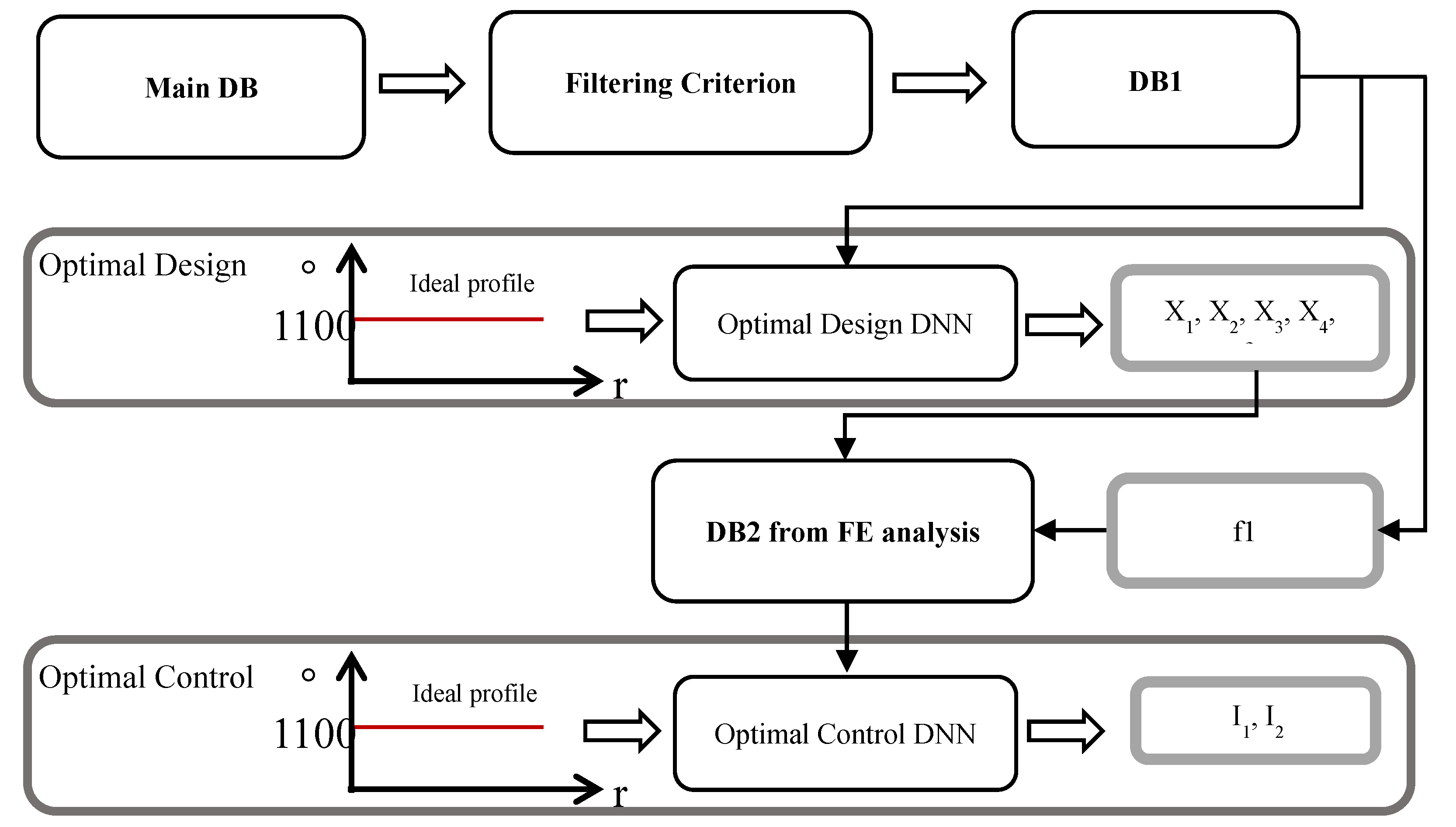
Figure 8.
Predicted vs. actual values of the Optimal Design DNN.
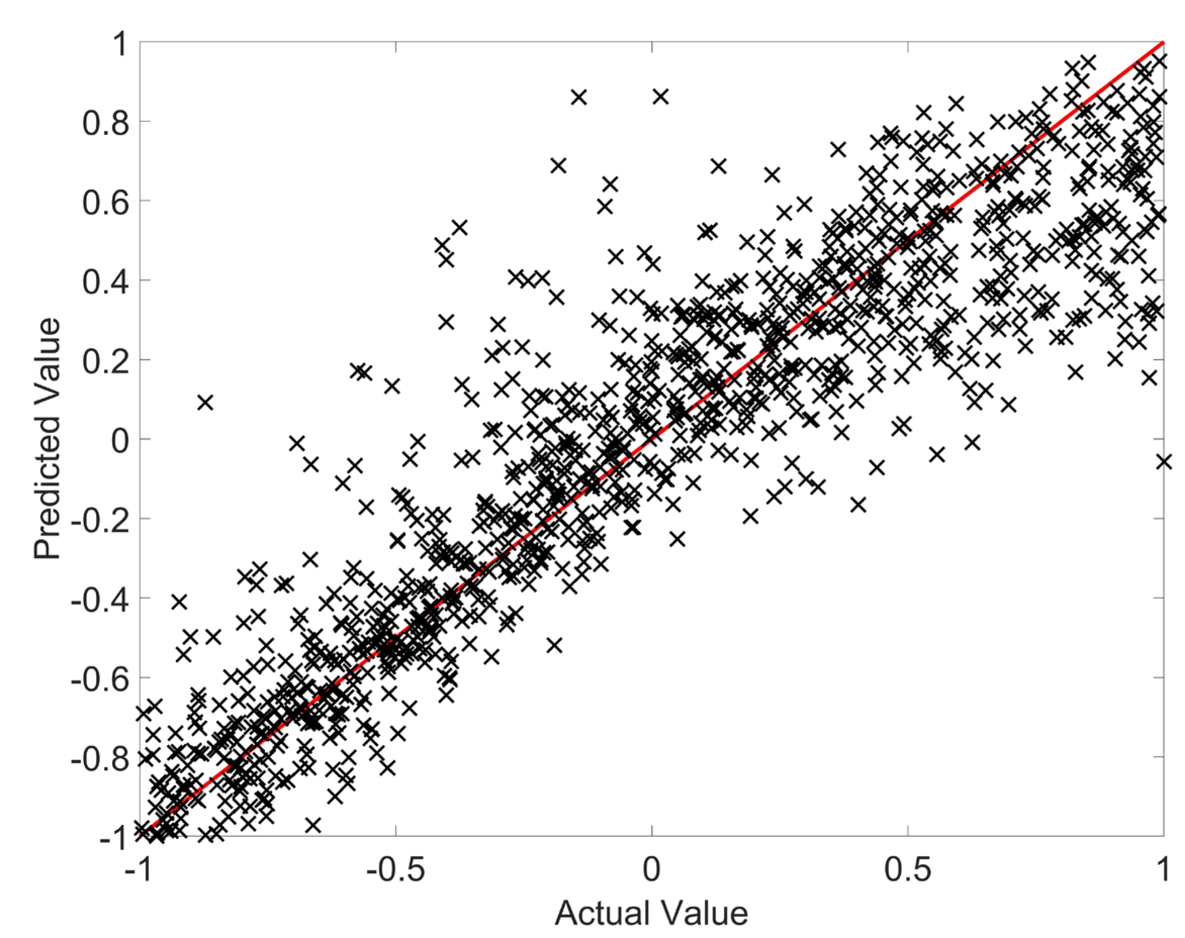
Figure 9.
Predicted vs. actual values of the Optimal Control DNN.
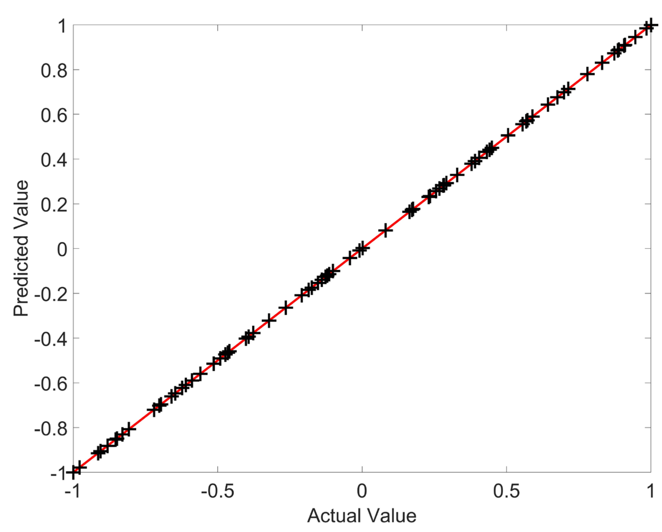
Figure 10.
Comparing the initial (left) and OD result’s (right) geometry.
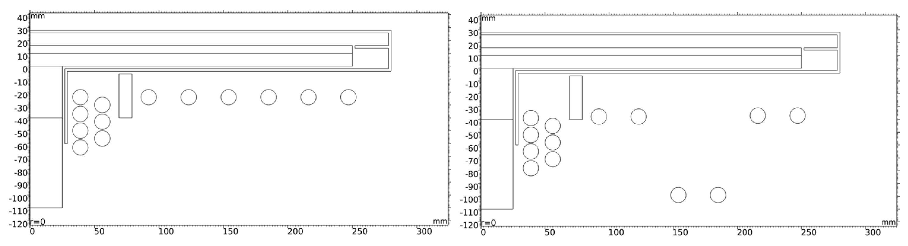
Figure 11.
Comparing the temperature distributions along the susceptor disk based on initial, OD result, and OC (optimized) results.
Figure 11.
Comparing the temperature distributions along the susceptor disk based on initial, OD result, and OC (optimized) results.
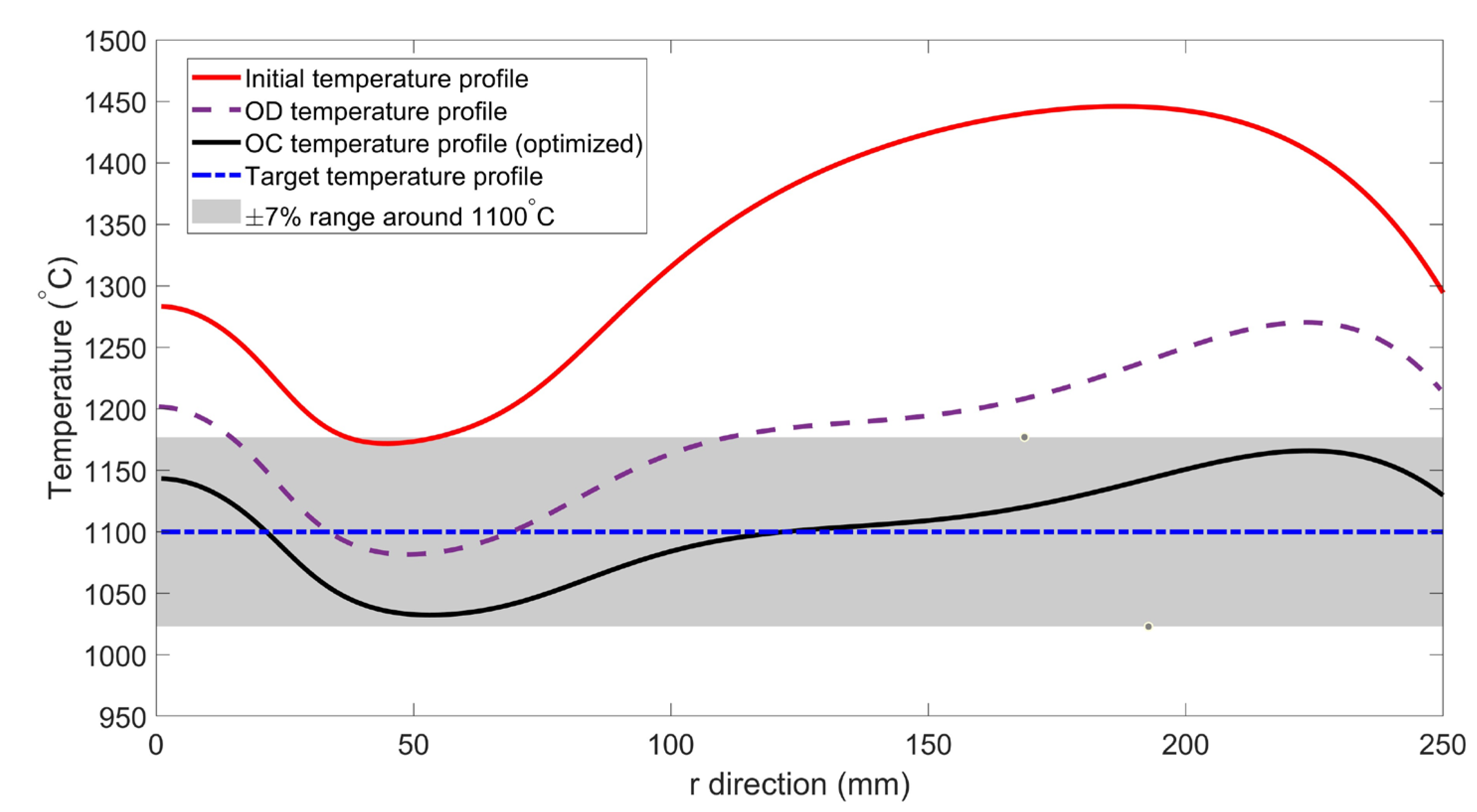

Table 1.
Material properties used in the models (electrical, magnetic and thermal ones).
| Material | Electrical properties | Magnetic properties | Thermal properties |
|---|---|---|---|
| Graphite disk | = 1.04 × 10⁵ S/m |
= 150 W/(m.K) = 10 W/(m2K) ε = 0.8 |
|
| Coils copper | = 5.998 × 10⁷ S/m | - | |
| Ferrite ring | = 10-9 S/m | - | |
| Air | = 0 S/m | = 850 ˚C | |
| Quartz | = 10-12 S/m | = 3 W/(m.K) |
Table 2.
Design variables with their range.
| Variables | Minimum | Maximum | Unit |
|---|---|---|---|
| I1 | 500 | A | |
| I2 | 400 | 2000 | A |
| f1 | 20 | 100 | kHz |
| f2 | 1 | 8 | kHz |
| x1 | 30 | 75 | mm |
| x2, x3, x4 | 11 | 100 | mm |
Table 3.
Optimal Design DNN structure.
| Layer | Number of neurons | Activation function |
|---|---|---|
| Input (Temperature profile) | 250 | -- |
| Hidden Layer 1 | 128 | Tan-Sigmoid |
| Hidden Layer 2 | 64 | Tan-Sigmoid |
| Hidden Layer 3 | 32 | Tan-Sigmoid |
| Hidden Layer 4 | 15 | Tan-Sigmoid |
| Output (x1…x4, f2) | 5 | Linear |
Table 4.
Optimal Design DNN assessment.
| Data sets | MAPE (%) | RMSE | |
|---|---|---|---|
| Training Set | 0.948 | 199.8 | |
| Validation Set | 17.8 | 0.950 | 196.9 |
| Test Set | 17.9 | 0.948 | 199.2 |
Table 5.
Optimal Design Results.
| Variable | OD phase Value | Initial Value | Unit |
|---|---|---|---|
| x1 | 43 | mm | |
| x2 | 37.8 | 24 | mm |
| x3 | 99 | 24 | mm |
| x4 | 37 | 24 | mm |
| f1 | 59984 | 60000 | Hz |
| f2 | 5112 | 5000 | Hz |
Table 6.
Optimal Control DNN structure.
| Layer | Number of neurons | Activation function |
|---|---|---|
| Input (Temperature profile) | 250 | -- |
| Hidden Layer 1 | 30 | Tan-Sigmoid |
| Hidden Layer 2 | 15 | Tan-Sigmoid |
| Hidden Layer 3 | 10 | Tan-Sigmoid |
| Hidden Layer 4 | 5 | Tan-Sigmoid |
| Output (I1, I2) | 2 | Linear |
Table 7.
Optimal Control DNN assessment.
| Data sets | MAPE (%) | RMSE | |
|---|---|---|---|
| Train Set | 1 | 0.02 | |
| Validation Set | < 0.01 | 1 | 0.04 |
| Test Set | < 0.01 | 1 | 0.05 |
Table 8.
Optimal Control Results.
| Variable | OC phase Value | Initial Value | Unit |
|---|---|---|---|
| I1 | 420 | 500 | A |
| I2 | 992 | 1200 | A |
Disclaimer/Publisher’s Note: The statements, opinions and data contained in all publications are solely those of the individual author(s) and contributor(s) and not of MDPI and/or the editor(s). MDPI and/or the editor(s) disclaim responsibility for any injury to people or property resulting from any ideas, methods, instructions or products referred to in the content. |
© 2025 by the authors. Licensee MDPI, Basel, Switzerland. This article is an open access article distributed under the terms and conditions of the Creative Commons Attribution (CC BY) license (https://creativecommons.org/licenses/by/4.0/).
Copyright: This open access article is published under a Creative Commons CC BY 4.0 license, which permit the free download, distribution, and reuse, provided that the author and preprint are cited in any reuse.


