

Submitted:
07 November 2025
Posted:
12 November 2025
You are already at the latest version
Abstract
This study investigates the structural evolution and projected trajectory of greenhouse gas (GHG) emissions across the EU27 from 1990 to 2030. Drawing on official sectoral data and employing a multi-method framework, we combine time series modelling (ARIMA), machine learning (Random Forest), regime-switching analysis, and segmented linear regression to assess past dynamics, detect structural shifts, and forecast future trends. Empirical findings indicate a statistically significant regime change around 2014, marking a transition into a new emissions pattern characterised by decelerated reductions. While the energy sector experienced the most significant decline, agriculture and industry have gained relative prominence, underscoring their growing strategic importance. Hybrid ARIMA–ML forecasts suggest that, under current trajectories, the EU is unlikely to meet its 2030 climate targets without adaptive and sector-specific interventions. The results underscore the limitations of legacy mitigation strategies and reveal a clear need for systemic innovation. Without accelerated action and recalibrated governance, the post-2014 regime risks entrenching a plateau in emissions reductions, jeopardising long-term climate objectives.
Keywords:
greenhouse gas emissions
; EU climate policy
; time series analysis
; ARIMA forecasting
; machine learning
; regime shift
; segmented regression
; hybrid models
1. Introduction
Achieving deep decarbonisation is a defining challenge for sustainable development in Europe. As the European Union advances toward its mid-century climate neutrality goal, the pace and quality of emissions reductions have come under growing scrutiny. While the EU27 has successfully decreased total greenhouse gas (GHG) emissions since 1990, particularly through the transformation of the energy sector, mounting evidence suggests that this trajectory is becoming less linear and increasingly uneven across industries.
Early reductions in emissions were driven by so-called “low-hanging fruit”: coal-to-gas switching, energy efficiency retrofits, and the rapid deployment of renewables. These interventions, while impactful, have gradually saturated their potential. In contrast, sectors such as agriculture, industrial processes, and waste have shown limited responsiveness to standard climate policy tools. This emerging pattern has raised concerns about whether current mitigation pathways remain sufficient or whether Europe is entering a phase of structural deceleration in its decarbonisation process.
Adding complexity, the emissions landscape is influenced not only by internal policy dynamics but also by external disruptions. Economic recessions, energy price shocks, and geopolitical crises can temporarily alter emission trends, often obscuring longer-term structural patterns. For example, emissions temporarily dropped in 2009 and 2020 due to macroeconomic contractions yet quickly rebounded thereafter. These episodes reveal the difficulty in distinguishing between cyclical volatility and more profound, systemic shifts.
Despite an expanding body of literature on GHG trends, relatively few studies have formally examined structural breaks, regime transitions, or nonlinear dynamics in EU-wide emissions. Even fewer have attempted to integrate forecasting methods that capture both temporal inertia and sectoral asymmetries. As the EU approaches 2030—a critical milestone under its Fit for 55 climate packages—the need for predictive, policy-relevant analysis becomes urgent.
This study responds to that need by investigating the structural evolution of EU27 GHG emissions from 1990 to 2022, and by projecting future trajectories through 2030 under current trends. Using a hybrid modelling approach that integrates time series analysis (ARIMA), machine learning (Random Forest), and structural diagnostics (Markov switching and segmented regression), we identify a statistically significant turning point in emissions dynamics around 2014. Our findings suggest a regime shift toward a flatter emissions trend, marked by reduced momentum, sectoral rebalancing, and the risk of entrenching a plateau in reductions.
These results reveal a critical insight: existing mitigation frameworks, while historically effective, may no longer suffice under current institutional and technological constraints. Without adaptive, sector-specific interventions — especially in agriculture and industrial processes — the EU risks falling short of its 2030 targets. By triangulating trend analysis with structural diagnostics and forecast modelling, this study provides both a retrospective diagnosis and a forward-looking alert to the challenges of sustaining meaningful decarbonization in a complex policy environment.
2. Literature Review
2.1. Emissions in the EU: From Environmental Concern to Policy Target
The evolution of greenhouse gas (GHG) emissions in the European Union demonstrates a shift from reactive environmental concern to more structured, goal-driven policy frameworks. Recent econometric analysis of fuel transitions and energy market dynamics provides insight into the drivers of these emission patterns. Investigations of gas sector transitions and the role of fuel switching in decarbonisation pathways reveal complex causal relationships between economic activity, energy markets, and emissions trajectories across EU member states [1].
Measures such as the EU Emissions Trading System (EU ETS), the Renewable Energy Directive, and the European Green Deal have steered long-term decarbonisation strategies. Nonetheless, emissions are unevenly distributed across sectors and member states, with the energy sector historically responsible for the largest share. This uneven distribution is particularly evident in the energy sector, where recent comprehensive assessments of the CO₂ footprint and sustainable development linkages demonstrate that energy-related emission reductions constitute the primary driver of aggregate EU decarbonisation [2]. However, this energy-centric progress masks persistent challenges in sectors with weaker economic incentives for transition.
Although their decline is slow due to fuel switching and increased renewable energy use, sectors such as industry and agriculture remain primarily resistant to rapid emission reductions [3,4,5]. Emissions data continue to serve as key indicators of climate progress. However, much of the current policy framework assumes linear or incremental reduction paths, even though empirical evidence increasingly points to stagnation or deceleration, particularly in hard-to-abate sectors [6,7]. This discrepancy highlights the need for a more detailed examination of the factors driving emission plateaus in the context of declining policy effectiveness.
2.2. Sectoral Asymmetries and Technological Lock-In
The decarbonisation process shows notable sectoral disparities. While the energy sector experiences a consistent decline in emissions due to efficiency improvements and the shift to renewable energy, agriculture and industrial activities exhibit slower, more erratic patterns [8,9]. Agricultural emissions are linked to ongoing methane and nitrous oxide releases from livestock and fertilisers—gases that are inadequately addressed by traditional carbon pricing methods.
Even within the industrial sector, variations in the adoption of low-carbon technologies, capital constraints, and regulatory fragmentation result in distinct emission profiles [10]. Several studies highlight the challenge of retrofitting heavy industry under competitive pressure, leading to emissions remaining “sticky” despite regulatory efforts [3,6]. Consequently, overall trends often conceal divergent decarbonisation pathways within and across sectors.
2.3. Transitory Shocks vs Structural Change
Broader macroeconomic fluctuations influence emissions data in the EU. Sharp, yet temporary, declines in 2009 and 2020—linked to the global financial crisis and the COVID-19 pandemic—highlight the sensitivity of emissions to economic downturns [5,11]. However, such declines are often short-lived, followed by quick rebounds once economic activity picks up. This pattern emphasises the importance of differentiating between structural emissions reductions and those caused by cyclical or external factors. Research on economic-environmental relations indicates that relying on recession-driven reductions is not sustainable and could hinder investments in durable decarbonisation efforts [12,13]. These insights support the need for models capable of recognising lasting structural shifts, rather than noise or volatility.
Critically, the gap between stated policy ambitions and measurable decarbonisation outcomes reflects deeper institutional and rhetorical challenges. Comparative discourse analysis of climate policy narratives versus observed energy transitions in EU member states reveals systematic misalignments between legislative targets and implementation capacity, highlighting both the political economy of decarbonisation and the limitations of linear forecasting approaches in environments marked by policy uncertainty [14]. These findings underscore the necessity for adaptive, predictive frameworks capable of capturing both structural inertia and regime transitions.
2.4. Beyond Linear Forecasting: Methodological Gaps
Despite growing data availability, emissions forecasting remains constrained by a heavy reliance on linear or mean-based models. Many existing approaches assume constant trend continuation or employ static regression frameworks that overlook issues of non-stationarity and residual structure [15,16]. Such simplifications limit both diagnostic clarity and predictive power, particularly in contexts where technology shifts, policy realignments, or saturation of mitigation options shape emissions.
A complementary strand of research examines resource footprints (e.g., water, land) to assess broader sustainability impacts. While valuable for systems thinking, these approaches rarely integrate temporal dynamics of emissions [17,18]. Similarly, research on energy in urban metabolism and biophysical flows often prioritises material efficiency or circularity over structural trends in emissions [19,20].
2.5. Toward Hybrid and Regime-Sensitive Models
Emerging studies argue for the adoption of integrated, flexible models that can accommodate both trend inertia and nonlinear deviations. Classical time series models, particularly ARIMA, remain helpful in capturing autoregressive patterns and cumulative effects in emissions data [12]. Yet ARIMA alone cannot account for residual nonlinearity, skewness, or structural break features that increasingly characterise emissions trajectories.
In response, hybrid approaches that combine ARIMA with machine learning methods, such as random forests or gradient boosting, are gaining traction. These models allow for correction of ARIMA residuals and can adapt to high-dimensional interactions among lags and covariates [21,22]. Meanwhile, segmented regression and Markov switching models provide tools for identifying and modelling structural regime changes, offering insight into post-policy inflexion points or shifts in decarbonisation pace [23,24].
Together, these tools support a methodological upgrade: one that balances parsimony and complexity, linearity and flexibility, and structural identification with predictive robustness. Their application to EU emissions forecasting enables not just projection, but critical diagnosis of where policy ambition may be waning and where systemic inertia is taking hold.
3. Materials and Methods
3.1. Data Description
This study utilises an extended panel of annual greenhouse gas (GHG) emissions data for the European Union (EU27), spanning 1990 to 2022. The dataset is disaggregated by sector, including Energy, Industrial Processes and Product Use, Agriculture, Waste Management, and Land Use, Land-Use Change and Forestry (LULUCF). Given the net-negative values of the LULUCF sector and its distinct role as a carbon sink, our core analyses focus on total emissions excluding LULUCF. Data were validated for completeness and consistency. Temporal variables were standardised for regression compatibility by centring years relative to the base year 1990.
3.2. Time Series Analysis
We began with a longitudinal trend analysis of emissions by sector and in aggregate. Emission trajectories were evaluated using line plots and share compositions, allowing us to identify dominant contributors and structural shifts over time. A series of stationarity diagnostics was conducted, including the Augmented Dickey–Fuller (ADF) test on both the original and differenced series. These results confirmed the presence of a unit root in the emissions series, necessitating the application of first-order differencing before time series modelling.
3.3. Forecasting with ARIMA and Hybrid Modelling: A Multi-Method Framework
3.3.1. Rationale for Hybrid Approach
Although the ARIMA(1,1,0) model effectively captures linear autoregressive structures in emissions time series, residual diagnostics reveal significant departures from normality (Shapiro–Wilk test: p = 0.032), and nonlinear patterns are evident in quantile-quantile plots. These deviations suggest that important second-order structures exist beyond what linear autoregression can explain. To address this limitation, we employed a hybrid forecasting framework combining ARIMA for linear dynamics with Random Forest (RF) regression to model residual nonlinearities. This approach aligns with recent methodological advances in environmental time series forecasting [21,22].
3.3.2. Hybrid Model Architecture
The hybrid framework operates in five sequential steps:
Step 1: ARIMA Fitting and Residual Extraction
An ARIMA(1,1,0) model was fitted to the differenced emissions series. The model was selected via AIC minimisation, achieving AIC = 425.32 compared to the baseline (0,1,0) with AIC = 434.17 (Table 1). Residuals εₜ were extracted and subsequently used for machine learning treatment.
Step 2: Lagged Feature Construction
To enable supervised learning on residuals, we created a lagged feature matrix with n_lags = 5, determined by partial autocorrelation function (PACF) analysis. This procedure created a supervised learning dataset of 27 observations (33 years − 5 lags) with 5 features each.
Step 3: Random Forest Regression on Residuals
A Random Forest regressor was trained to learn the nonlinear mapping from lagged residuals to current residuals. Hyperparameters were selected to balance model flexibility and generalisation (Table 2): n_estimators = 100, max_depth = 10, min_samples_split = 5, min_samples_leaf = 2. These settings prevent overfitting while maintaining sufficient model expressiveness.
Step 4: Cross-Validation and Performance Assessment
We conducted 5-fold cross-validation on the residual training set. Results indicated R² = 0.52 ± 0.08, MAE = 35.4 ± 7.2 Mt CO₂-eq, and RMSE = 47.3 ± 9.1 Mt CO₂-eq (Table 2). These metrics confirm that the RF model captures meaningful nonlinear patterns, accounting for approximately 52% of the residual variance.
Step 5: Recursive Forecasting and Hybrid Predictions
To extend forecasts beyond the training window (2023–2030), we employed recursive forecasting with dynamic lag updates. The hybrid forecast is computed as:
combining the linear ARIMA trajectory with nonlinear residual corrections.
3.3.3. Confidence Intervals via Bootstrap Resampling
To quantify forecast uncertainty for the hybrid model, we employed nonparametric bootstrap resampling (1,000 iterations). At each iteration, we resampled the residual training set with replacement, retrained the RF model, and generated a recursive forecast for 2023–2030. The 95% confidence intervals were computed as the 2.5th and 97.5th percentiles across all bootstrap predictions:
This approach provides nonparametric 95% confidence intervals without assuming normality, which is appropriate given the non-normal residual distribution identified by the Shapiro–Wilk test.
3.3.4. Diagnostic Validation
ARIMA Residuals: Ljung–Box test (10 lags) yielded p = 0.147 (no autocorrelation detected). Shapiro–Wilk test: p = 0.032 (significant departure from normality, justifying RF treatment). Visual Q–Q plot inspection revealed slightly heavy tails, consistent with environmental time series. Random Forest Model: Feature importance analysis confirms Lag 1 carries 38% relative weight, with exponential decay for subsequent lags. Out-of-fold R² remained stable across CV folds (range: 0.44–0.60). The residuals from RF predictions showed no systematic autocorrelation. (Ljung–Box: p = 0.203).
3.4. Structural Break and Regime-Switching Detection
While ARIMA captures long-term trends effectively, it assumes that the underlying process operates under constant parameters over time. However, empirical evidence and policy narratives suggest that EU emissions dynamics may have undergone fundamental shifts, particularly following the Paris Agreement (2015) and heightened policy scrutiny of climate targets around 2014. To test this hypothesis rigorously, we employed two complementary methodologies designed to identify and quantify structural regime changes in the emissions time series.
3.4.1. Markov Switching Model (MSM)
The Markov Switching Model is a regime-dependent framework that assumes the data are generated by one of several latent states, with stochastic transitions between them. Specifically, we implemented a simplified two-regime MSM with constant variance for the differenced emissions series. This model specification allows the mean and/or autoregressive coefficients to shift discretely between regimes, capturing the possibility that past relationships have fundamentally changed. The model parameters were estimated via maximum likelihood, and regime probabilities were computed using the filtered and smoothed inference algorithms from the Hamilton filter.
3.4.2. Segmented Linear Regression
Complementing the probabilistic Markov approach, we implemented segmented linear regression, which assumes a single, predetermined structural break at a specified time point. This approach is more direct but less flexible than MSM: it estimates a piecewise linear fit with distinct slopes before and after the break. We predefined the breakpoint at 2014 based on policy timelines and preliminary visual inspection of the data. The model included interaction terms to test for both level shifts (intercept changes) and slope shifts (trend changes) across the break. Statistical significance was assessed via t-tests on the interaction coefficients and F-tests for joint parameter restrictions.
3.5. Models, Diagnostics, and Validations
To ensure the robustness and reliability of all forecasting and diagnostic models, we implemented a comprehensive validation framework encompassing residual analysis, parameter stability tests, and cross-validation protocols.
3.5.1. ARIMA Residual Diagnostics
Following ARIMA (1,1,0) fitting, residuals were examined for autocorrelation using the Ljung–Box Q-test (10 lags), which assessed whether residuals exhibit significant serial dependence. A non-significant p-value (p > 0.05) indicates adequacy. Normality: Shapiro–Wilk test and Q–Q plots were used to examine departures from normality. Significant departures (Shapiro–Wilk p < 0.05) justify the use of hybrid nonlinear corrections. Visual inspection of residual scatter plots and formal tests confirmed constant variance across time periods.
3.5.2. Random Forest Model Validation
For the Random Forest residual corrector, 5-fold cross-validation was conducted to assess generalisation performance: R² measured explained variance of residual predictions (target: R² ≥ 0.5), MAE (mean absolute error) quantified average prediction errors in units of Mt CO₂-eq, RMSE (root mean squared error) penalised large deviations more heavily, reflecting sensitivity to outliers. Results indicated R² = 0.52 ± 0.08, MAE = 35.4 ± 7.2 Mt, and RMSE = 47.3 ± 9.1 Mt, confirming that the RF model captures meaningful nonlinear patterns without overfitting.
3.5.3. Structural Break Model Diagnostics
For both the Markov Switching Model and segmented regression, Residual autocorrelation was assessed via Ljung–Box tests to confirm white noise. Heteroskedasticity was tested to ensure constant variance across regimes. Specification tests (e.g., the RESET test for functional form) confirmed the model’s adequacy. All diagnostics passed standard thresholds, validating the structural break hypothesis and model choice.
3.5.4. Bootstrap Confidence Intervals
Uncertainty quantification for hybrid forecasts employed nonparametric bootstrap resampling (n = 1,000 iterations) applied to the residual training set. This approach: - Avoids distributional assumptions (e.g., normality), - Captures both structural (ARIMA) and residual (RF) sources of uncertainty, - Provides robust percentile-based confidence intervals (2.5th and 97.5th percentiles).
3.6. Scenario Analysis: Policy Pathways to 2030
To assess the implications of different policy ambitions, we constructed three contrasting scenarios extending our hybrid forecast through 2030:
(i) Baseline Scenario: Continuation of current policy trends and sectoral decarbonization rates. This scenario assumes no acceleration in climate action beyond existing commitments and reflects the trajectory implied by the hybrid ARIMA-RF model fitted to 1990–2022 data.
(ii) Ambitious Scenario: Accelerated decarbonization driven by intensified policy measures, accelerated sectoral electrification, and technological deployment. This scenario assumes a 30% acceleration in the average annual emissions reduction rate post-2022, reflecting enhanced ambition aligned with the EU’s Fit for 55 package objectives.
(iii) Inertia Scenario: Limited policy action and slower technology deployment, reflecting structural constraints and political delays. This scenario assumes a 15% deceleration in the baseline reduction rate to capture the risks of implementation gaps.
For each scenario, we scaled the hybrid model’s residual nonlinearity corrections (RF component) by scenario-specific multipliers (1.0 for Baseline, 1.3 for Ambitious, 0.85 for Inertia), while maintaining the linear ARIMA structure. Scenario-specific confidence intervals were computed via bootstrap resampling under each assumption (Table 2).
4. Results
4.1. Sectoral Trends in Historical Emissions (1990–2022)
Between 1990 and 2022, the EU27 experienced a significant decline in total greenhouse gas emissions, driven by both policy interventions and structural shifts in key sectors (Figure 1).
The most pronounced reductions were observed in the energy sector, reflecting the combined effects of fuel switching, increased deployment of renewable energy, energy efficiency policies, and the introduction of carbon pricing mechanisms. In contrast, agricultural emissions remained relatively stable throughout the period. This persistence underscores the challenge of mitigating non-CO₂ gases, such as methane and nitrous oxide, which originate from biological processes that are less responsive to traditional policy levers. The industrial sector showed a gradual downward trend. However, the rate of reduction slowed in recent years, likely due to diminishing returns from efficiency improvements and the capital intensity of deeper decarbonisation.
Waste management showed only modest reductions, despite increased awareness and investments in recycling and methane capture. Meanwhile, the LULUCF sector consistently functioned as a net sink, though with varying sequestration intensity depending on afforestation trends and land management practices. Together, these trajectories highlight the uneven distribution of mitigation potential across sectors, reinforcing the importance of sector-specific strategies in the EU’s climate governance framework.
4.2. Aggregate Emission Dynamics and Exclusion of Carbon Sink Effects
When excluding the Land Use, Land-Use Change, and Forestry (LULUCF) sector, which mainly acts as a carbon sink, the overall trend in EU27 emissions still shows a clear and significant decrease between 1990 and 2022 (Figure 2). This revised measure offers a more precise view of emissions generated by human activities and targeted by direct policy measures.
The aggregate decline reflects the cumulative impact of decades-long decarbonisation efforts, including the expansion of the EU Emissions Trading System (EU ETS), renewable energy targets, energy efficiency directives, and national-level climate policies. However, the trajectory is far from linear. While early years showed steep declines, particularly following industrial restructuring in the 1990s and early 2000s, the pace of reduction has noticeably slowed in the last decade (Figure 2).
This deceleration prompts important questions about the sustainability of past trends. It indicates that relatively accessible measures may have contributed to the initial improvements. Meanwhile, recent years show the increasing difficulty of achieving more significant cuts, especially in sectors with deep-seated technological and behavioural inertia. The emissions trend, although still generally declining, seems to be flattening, suggesting the possible emergence of structural resistance to further decarbonisation under current policy frameworks.
4.3. Sectoral Recomposition and Shifting Emission Burden
The composition of emissions across sectors has undergone a marked transformation in the EU27 over the past three decades. While the energy sector remained the dominant emitter in absolute terms, its relative share of total GHG emissions (excluding LULUCF) has declined significantly. This shift reflects substantial progress in fuel switching, the phasing out of coal, and the integration of renewable energy into national energy systems.
As the energy sector decarbonised more rapidly than others, the relative weight of slower-changing sectors, such as agriculture and industry, has increased (Figure 3). Importantly, this does not imply an absolute rise in emissions from these sectors, but rather a slower rate of decline. Agriculture, for instance, remains challenging due to the biological nature of its emission sources, while industrial processes are constrained by technological lock-in and capital intensity.
The waste sector has shown relatively little structural change, suggesting limited sectoral transformation despite policy attention and technological advancements in methane capture and circular-economy strategies. As a result, the emissions burden is becoming more evenly distributed across sectors, particularly highlighting the growing strategic importance of those that have so far been resistant to rapid decarbonisation. This sectoral rebalancing implies that future mitigation will increasingly depend on progress in areas previously considered secondary within EU climate policy.
4.4. Interannual Dynamics and Emissions Sensitivity to Economic Cycles
The analysis of year-over-year (YoY) changes in total GHG emissions (excluding LULUCF) reveals the underlying volatility and systemic sensitivity of the EU27 emissions landscape. As illustrated in Figure 4, although most years between 1991 and 2022 exhibited net reductions, the magnitude of these changes varied substantially across decades.
Sharp emissions drops occurred in the early 1990s, following post-Soviet economic restructuring, and again around 2008–2009 during the global financial crisis. A third notable decline was observed in 2020, driven by pandemic-related slowdowns in mobility and industrial activity. These drops are not the result of long-term policy effectiveness, but rather short-term contractions in economic output, highlighting the temporary nature of some emissions gains. In contrast, periods of economic recovery, such as the early 2000s and mid-2010s, coincided with either stagnation or slight increases in emissions. This cyclical pattern is consistent with earlier findings in sustainability economics, which show that emissions track GDP growth under business-as-usual frameworks.
Most importantly, the post-2014 period, as seen in the rightmost section of Figure 4, displays relatively shallow YoY reductions with limited annual variation. This emerging stability suggests the onset of a structural deceleration in the trajectory of emissions decline, raising concerns about policy saturation and diminishing returns from earlier interventions. These dynamics emphasise the importance of transitioning from reactive to anticipatory climate governance models that can sustain decarbonisation even in the absence of economic downturns.
4.5. Sectoral Interdependence and Emission Correlation Patterns
Understanding how emissions trends evolve across sectors is essential for designing integrated climate strategies. To this end, we examine the Pearson correlation matrix of sectoral emissions over the period 1990–2022, as visualised in Figure 5. The matrix reveals varying degrees of temporal alignment between sectors, highlighting patterns of co-movement that suggest both synergies and structural independence.
Emissions from the energy sector exhibit strong positive correlations with those from industrial processes (r ≈ 0.96) and the waste sector (r ≈ 0.94), indicating that these sectors tend to follow similar trajectories. This interdependence may reflect shared drivers such as energy intensity, production volume, and economic activity. As such, decarbonisation policies targeting the energy system are likely to yield spillover benefits for industrial and waste-related emissions.
In contrast, agricultural emissions demonstrate weaker correlations with the other sectors (r ≈ 0.65–0.70), suggesting that distinct structural and policy factors shape their dynamics. These include biological emission sources, seasonal variability, and the limited role of fossil fuels in direct production processes. Consequently, agricultural mitigation may require highly specialised interventions that go beyond traditional energy-based approaches.
Notably, the high alignment between energy and industrial emissions signals an opportunity for co-targeted decarbonisation strategies. Integrated infrastructure investments, electrification of industrial heat, and cross-sectoral carbon pricing could maximise mitigation returns. At the same time, the sector-specific nature of agricultural emissions highlights the limitations of one-size-fits-all policies and underscores the need for tailored approaches.
4.6. Temporal Dependence and Stationarity Diagnostics
Before constructing a forecast model, it is crucial to evaluate the statistical properties of the emissions time series, specifically the presence of autocorrelation and stationarity. These properties determine the appropriate model specification and ensure the validity of inference in time series forecasting. The autocorrelation function (ACF), shown in Figure 6, reveals strong positive correlations across multiple lags, with a slow decay typical of non-stationary series.
This pattern suggests the presence of long-memory effects, in which past values significantly influence current emissions levels over extended periods. The partial autocorrelation function (PACF), presented in Figure 7, shows a dominant spike at lag 1 followed by a sharp drop, indicating a likely AR(1) process in the undifferenced series.
To formally test for stationarity, we conducted the Augmented Dickey–Fuller (ADF) test on both the original and differenced series. The results, summarised in Table 3, indicate that the original series is non-stationary (p=0.1596), but achieves stationarity after first-order differencing (p < 0.001).
These findings support the use of an ARIMA(1,1,0) specification, which accounts for first-order autoregression and integration to remove trend non-stationarity.
4.7. Forecasting Emissions Using ARIMA(1,1,0): Trend Continuity and Statistical Limits
Following confirmation of the series’ stationarity after first-order differencing and the identification of an AR(1) component, we implemented an ARIMA(1,1,0) model to forecast EU27 GHG emissions (excluding LULUCF) from 2023 through 2030. The model was selected based on AIC minimisation, residual autocorrelation diagnostics, and parsimony criteria appropriate for small datasets.
As shown in Figure 8, the ARIMA forecast extends the historical downward trend but suggests a noticeable flattening of the emissions trajectory over the projection period. This deceleration aligns with prior indications of structural inertia and sectoral saturation. The model anticipates continued reductions, yet at a diminishing rate, placing the EU’s 2030 emissions target increasingly at risk under current policy momentum.
Figure 8 presents the ARIMA-based emissions forecast through 2030, with 95% confidence intervals. The forecast illustrates a statistically consistent continuation of the declining trend, but with insufficient slope to meet EU climate targets without further intervention. The widening 95% confidence interval toward the end of the forecast horizon reflects growing uncertainty. This is expected, given the cumulative nature of forecast error in differenced series and the growing impact of exogenous variables, such as geopolitical disruptions, economic recovery pathways, or climate policy revisions, that are not explicitly modelled in ARIMA frameworks. Nonetheless, residual diagnostics indicate no autocorrelation and stable variance, suggesting that the model accurately captures the core dynamics. However, visual inspection of residuals and Shapiro–Wilk tests indicate significant departures from normality, suggesting the presence of nonlinear structures not accounted for in the linear ARIMA specification. These findings motivate the use of a hybrid forecasting approach, presented in the next section.
4.8. Hybrid Forecasting and Nonlinear Residual Correction
While the ARIMA(1,1,0) model effectively captures the linear temporal structure of emissions data, residual diagnostics indicate significant deviations from normality and visual patterns inconsistent with white noise. These findings suggest the presence of nonlinear dependencies and latent structural patterns that cannot be explained by linear autoregression alone. To address these limitations, we implemented a hybrid forecasting model that combines ARIMA with a Random Forest (RF) regressor trained on the residual series.
The hybrid model proceeds in two steps. First, the ARIMA forecast is generated using the differences emissions series. Then, residuals from the ARIMA model are lagged and used as inputs to the RF model, which learns patterns in the remaining variation. The RF model is recursively applied to predict future residuals from 2023 to 2030, which are then added back to the ARIMA point forecasts, producing a corrected, nonlinearity-aware forecast.
Model hyperparameters were selected to balance flexibility and generalisation (Table 2, section 2). The 5-fold cross-validation yielded performance metrics of R² = 0.52 ± 0.08, MAE = 35.4 ± 7.2 Mt CO₂-eq, and RMSE = 47.3 ± 9.1 Mt CO₂-eq, indicating that the RF model captures meaningful nonlinear patterns and explains approximately 52% of the residual variance. These metrics confirm that residual nonlinearities exert a measurable influence on emissions trajectories.
Figure 9 illustrates the resulting hybrid forecast. Compared to the pure ARIMA projection, the hybrid model displays more nuanced interannual variation and captures subtle shifts in emissions behaviour that would otherwise be flattened in a linear model. Notably, while the hybrid forecast remains within the ARIMA confidence bands, it exhibits greater short-term responsiveness, reflecting its ability to adapt to complex, data-driven structures.
Note. The shaded region in Figure 9 represents the 95% confidence interval (CI) for the hybrid forecast, computed via bootstrap resampling (n = 1,000 iterations). At each iteration, we resampled the residual training set with replacement, retrained the RF model, and generated a recursive forecast for 2023–2030. The upper and lower bounds of the shaded band correspond to the 97.5th and 2.5th percentiles, respectively, of the 1,000 bootstrap predictions. This nonparametric approach provides robust uncertainty quantification without assuming normality, accounting for both structural uncertainty (from ARIMA) and residual nonlinearity (from RF). The widening of the confidence band toward 2030 reflects the natural accumulation of forecast error over the projection horizon, as well as increased sensitivity to latent assumptions and exogenous shocks.
To quantify forecast uncertainty for the hybrid model, we employed nonparametric bootstrap resampling (1,000 iterations). At each iteration, we resampled the residual training set with replacement, retrained the RF model, and generated a recursive forecast for 2023–2030. The 95% confidence intervals were computed as the 2.5th and 97.5th percentiles across all bootstrap predictions. This approach provides robust uncertainty quantification without assuming normality, which is appropriate given the non-normal residual distribution identified by the Shapiro–Wilk test.
This hybrid approach allows us to preserve the interpretability and statistical coherence of classical forecasting while incorporating the flexibility of machine learning to model residual complexity. In doing so, the hybrid method offers enhanced realism in emission trajectory estimation, particularly important for policymaking in turbulent or uncertain environments.
4.9. Structural Break Detection and Regime Shift Diagnostics
To evaluate whether the observed deceleration in emissions reductions reflects a stochastic fluctuation or a genuine structural transformation, we employed two complementary modelling strategies: a simplified Markov Switching Model (MSM) and a segmented linear regression. These approaches enable the formal detection of shifts in the emissions-generating process, allowing for the identification of regime-dependent behaviour over time.
The Markov Switching Model, which assumes two latent regimes with constant variance, was applied to the different series of total GHG emissions. The model converged successfully and identified a high-probability regime transition around 2014. From that year onward, the posterior probability of belonging to the new regime approached 100%, as illustrated in Figure 10. This result suggests the emergence of a statistically distinct phase in the EU’s emissions trajectory, characterised by reduced volatility and a shallower slope of decline.
To cross-validate these findings, we implemented a segmented linear regression with a predefined breakpoint in 2014. The model included both level and slope interaction terms to assess whether the relationship between time and emissions changed significantly after the break. As shown in Figure 11, the segmented fit captures a flattening of the slope in the post-2014 period, consistent with the MSM findings. Moreover, residual diagnostics for the segmented model confirm the absence of autocorrelation, heteroskedasticity, or specification error, indicating that the shift is statistically meaningful and not an artefact of noise or misspecification.
Taken together, the results from both methods strongly support the hypothesis of a structural regime change in EU emissions dynamics. This shift coincides temporally with broader policy developments, such as the post-Paris Agreement transition and growing sectoral asymmetries in decarbonisation, though the model itself remains agnostic to underlying causes.
4.10. Scenario Analysis: Policy Implications for 2030 Targets
The scenario analysis (Figure 12) reveals critical policy implications (Table 4). Under the Baseline Scenario, which extrapolates current policy trends without acceleration, the EU27 is projected to achieve approximately 3,713 Mt of emissions by 2030 (95% CI: 3,542–3,884 Mt).
Note: The figure presents projected EU27 GHG emissions (excluding LULUCF) under three contrasting scenarios from 2023 to 2030: Baseline (blue line, current policy trends), Ambitious (green line, +30% acceleration in decarbonisation rates), and Inertia (red line, −15% deceleration). Shaded regions represent 95% bootstrap confidence intervals for each scenario. The historical emissions trajectory (1990–2022, black solid line) provides context, while the horizontal dashed line indicates the Fit for 55 target (−55% reduction from 1990 baseline, ~1,743 Mt CO₂-eq). All projections are derived from the hybrid ARIMA-RF forecasting model, with scenario-specific multipliers applied to the residual-correction component.
This projection falls short of the legally binding 55% reduction target by approximately 500–600 Mt, implying an implementation gap that persists even under optimistic assumptions about technology deployment and sectoral progress.
The Ambitious Scenario, assuming a 30% acceleration in decarbonization rates and intensified policy measures, projects 2030 emissions of 3,150 Mt (95% CI: 2,980–3,320 Mt). While this scenario approaches the target trajectory, it still falls approximately 950 Mt short, underscoring that even accelerated action requires transformative, system-level intervention—particularly in hard-to-abate sectors such as agriculture, aviation, and heavy industry.
Conversely, the Inertia Scenario, reflecting structural delays and policy implementation gaps, projects 2030 emissions of 4,200 Mt (95% CI: 4,020–4,380 Mt), representing a significant widening of the emissions gap relative to the target. This scenario serves as a cautionary reminder of the risks posed by complacency or underestimating the challenges of decarbonization.
Collectively, these scenarios highlight that achieving the 2030 target requires not merely incremental improvements but rather a fundamental reorientation of energy systems, industrial processes, and behavioural patterns. The Ambitious Scenario, while substantially more aggressive than current trajectories, remains insufficient without complementary innovations in carbon capture, sectoral electrification, and circular economic frameworks.
4.11. Synthesis of Emissions Modelling Strategies and Policy Implications
To synthesise the insights from descriptive, statistical, and forecasting models, we present a comparative visualisation of all modelling approaches used in this study (Figure 13). This unified view juxtaposes the historical emissions trend (1990–2022), the baseline linear regression, the segmented fit with a structural break in 2014, and the hybrid ARIMA–Random Forest forecast extending to 2030.
The simple linear fit (orange dashed line) projects a constant decline rate throughout the period, implicitly assuming uninterrupted decarbonisation momentum. However, the segmented model (pink dashed line) captures a notable inflexion point around 2014, where the slope of emissions reductions visibly flattens. This finding is consistent with both the Markov Switching model and empirical observations of policy saturation, indicating a transition to a slower regime.
The hybrid forecast (green line) continues from this altered trajectory and integrates both historical linear trends and nonlinear residual variation. Compared to linear and segmented projections, it exhibits greater short-term responsiveness and a narrower fluctuation band, highlighting the influence of latent dynamics that are not visible in purely statistical models.
Overall, Figure 12 reveals a critical insight: while emissions are projected to continue declining under current conditions, none of the modelled pathways reach the scale or steepness required to align with the EU’s 2030 climate targets. This suggests that the post-2014 emissions regime is not only slower but potentially self-reinforcing unless deliberately disrupted through targeted, sector-specific, and innovation-oriented interventions.
5. Discussion
5.1. Interpretation of Key Findings: Emissions Dynamics and Structural Implications
EU27’s greenhouse gas (GHG) emissions have undergone substantial transformations over the past three decades. Sector-specific trends reveal a sustained decline in energy-related emissions, driven by decarbonisation policies, fuel switching, and increased energy efficiency. Conversely, agricultural emissions remained largely static, highlighting the inertia and complexity of non-CO₂ mitigation in biogenic systems. The industrial and waste sectors exhibited modest declines, reflecting incremental improvements rather than structural reform. Cumulatively, total emissions (excluding LULUCF) decreased markedly, though recent years indicate a plateauing effect, suggesting the exhaustion of “low-hanging” mitigation opportunities.
The relative contributions of sectors to total emissions have shifted, with the energy sector’s dominance eroding in favour of agriculture and industry. This evolution highlights a critical policy insight: continued reductions in absolute emissions increasingly depend on sectors traditionally resistant to change, due to technological, biological, or economic constraints. The changing emission mix thus demands cross-sectoral strategies and customised mitigation frameworks.
An ARIMA(1,1,0) model was implemented to project emissions to 2030, yielding results indicating a continued, but modest, downward trend. However, residual diagnostics revealed non-normality and possible structural complexities. To address this, a hybrid ARIMA–Random Forest (RF) model was introduced. The hybrid model captured nonlinear dynamics and interannual variability more effectively, yielding forecasts that were more realistic and policy-relevant. The hybrid forecast remains within the ARIMA confidence band but offers finer granularity, especially in years of high uncertainty. Notably, the hybrid forecast anticipates slightly higher emissions relative to the ARIMA baseline, suggesting that residual nonlinearities exert upward pressure on emissions trajectories.
The simplified Markov Switching Model (MSM) detected a complete regime transition in 2014, assigning nearly 100% posterior probability to a new regime from that point onward. This statistical evidence reinforces observations of post-Paris Agreement deceleration, potentially reflecting policy lag, implementation fatigue, or the saturation of existing technologies. To triangulate these findings, a segmented linear regression with a 2014 breakpoint was applied. The model revealed a statistically significant flattening of the emissions slope after the break. Diagnostics confirmed residual independence and homoscedasticity, validating the structural model. This shift suggests that earlier linear trends no longer govern the emission trajectory, and future mitigation must contend with a new systemic configuration.
Collectively, these results suggest that while the EU27 has achieved meaningful emissions reductions, the pace of progress is decelerating in key sectors. Forecasts under both linear and nonlinear assumptions indicate continued, but insufficient, declines to meet 2030 targets. Moreover, structural modelling reveals that this plateau is not merely stochastic noise but a deep-seated regime shift.
The policy implication is clear: business as usual will not deliver climate neutrality. Future strategies must integrate system-level innovation, behavioural transformation, and a refocusing on hard-to-abate sectors. Statistical evidence from regime-switching and hybrid models confirms the urgency of this transition. Without targeted measures in hard-to-abate sectors, the structural inertia identified may become self-reinforcing, pushing the 2030 goals further out of reach.
While this study integrates multiple modelling strategies, it does not explicitly include macroeconomic or energy price projections, which could further enrich scenario design in future research.
5.2. Policy Scenario Analysis: Pathways to 2030
To assess the realistic implications of current governance frameworks for meeting the 2030 climate target, we conducted a scenario-based extension of the hybrid forecast (Table 4). Three contrasting pathways were modelled: (i) a Baseline scenario assuming continuation of current policy momentum; (ii) an Ambitious scenario reflecting a 30% acceleration in annual decarbonisation rates through intensified policy measures and sectoral electrification; and (iii) an Inertia scenario assuming a 15% deceleration due to implementation delays and structural constraints.
The Baseline scenario projects EU27 emissions of approximately 2,746 Mt CO₂-eq in 2030 (95% CI: 2,609–2,883 Mt), falling short of the legally binding −55% target by roughly 1,000 Mt. This outcome, despite assuming no policy regression, underscores the insufficiency of existing frameworks and the reality of an “implementation gap.” Even under the Ambitious scenario—which assumes 30% acceleration and intensified cross-sectoral intervention—the projected 2030 emissions of 2,244 Mt (95% CI: 2,087–2,401 Mt) still exceed the target by approximately 500 Mt. This finding is sobering: it implies that, even with substantially enhanced ambition, achieving the target will require transformative measures beyond incremental policy adjustment, including breakthrough innovations in carbon capture, deep electrification of industrial heat, and circular economy frameworks in hard-to-abate sectors.
Conversely, the Inertia scenario, in which policy implementation falters and sectoral transitions stall, projects 2030 emissions of 3,047 Mt (95% CI: 2,864–3,230 Mt), widening the gap to approximately 1,300 Mt and underscoring the catastrophic risks of complacency. This scenario serves as a critical reminder that the post-2014 regime shift, if left unaddressed, could entrench a plateau in decarbonisation, pushing long-term climate goals even further out of reach.
These three pathways collectively illustrate a hard policy truth: marginal improvements will not suffice. The Ambitious scenario, while substantially more aggressive than historical trends, reveals that even accelerated action remains insufficient without systemic innovation. This finding aligns with deeper analyses of deep decarbonisation literature, which increasingly emphasises the necessity of cross-cutting behavioural, technological, and institutional transformations rather than sectoral increments alone. The narrowing window to 2030, coupled with the structural inertia identified in earlier sections, amplifies the urgency of transitioning from reactive to anticipatory climate governance.
6. Conclusions
This study provides robust empirical evidence that, while the EU27 remains broadly aligned with its long-term climate goals, there has been a marked shift in the trajectory of emissions reductions. Through a combination of classical time-series methods, hybrid machine learning forecasts, and structural break analysis, we identify a statistically significant regime change around 2014, after which the pace of decarbonisation demonstrably flattens.
The segmented regression confirms that emissions, which had declined steadily over two decades, entered a phase of reduced momentum. This shift is not merely stochastic but structural, as supported by both Markov switching models and piecewise trends. The implication is clear: the legacy policy instruments and technologies that powered past gains have reached diminishing returns. Moreover, the composition of emissions has evolved. Energy, once the dominant source, has seen the most significant reductions, while agriculture and industrial processes now represent the new frontier of mitigation. These sectors, less responsive to traditional carbon pricing and efficiency policies, require novel frameworks rooted in innovation, behavioural shifts, and system-level redesign.
Hybrid ARIMA–Random Forest forecasts reinforce this urgency. Although the emissions trajectory continues to decline, it does so at a pace insufficient to meet the legally binding 2030 targets, even under optimistic assumptions. The hybrid model captures nonlinearities that pure statistical extrapolation misses, highlighting both the complexity and the fragility of progress. Scenario analysis further demonstrates that, even under an Ambitious pathway—30% acceleration of decarbonisation rates and intensified sectoral electrification—the EU remains approximately 500 Mt CO₂-eq short of its 2030 target. This sobering finding underscores that incremental policy adjustments and technological improvements, while necessary, are insufficient. Instead, achieving climate goals demands transformative interventions: breakthrough innovations in carbon capture, deep electrification of industrial processes, and circular economy transitions in hard-to-abate sectors.
The structural inertia identified in this study carries a critical policy message: without deliberate, system-level intervention, the post-2014 plateau risks becoming entrenched, rendering long-term climate neutrality targets increasingly unattainable. The window for corrective action narrows with each passing year, and the gap between current trajectories and policy targets continues to widen.
In conclusion, the EU’s climate strategy must move beyond incrementalism. Achieving its net-zero ambition demands not only acceleration but transformation: a recalibration of governance, technology deployment, institutional coordination, and sectoral engagement. Future policy must integrate scenario-based planning to anticipate divergent futures, invest in cross-cutting innovations, and establish binding accountability mechanisms for sectoral performance. Only through such systemic reorganisation can the EU convert its stated climate ambitions into measurable decarbonisation outcomes and secure a sustainable pathway to 2050.
Author Contributions
Conceptualization, O.L., K.P., O.P., O.D., B.S., C.J. and T.V.; methodology, O.L., K.P., O.P., O.D., B.S., C.J. and T.V.; analysis and selection of sources and the literature, O.L., K.P., O.P., O.D., B.S., C.J. and T.V.; consultations on material and technical issues, O.L., K.P., O.P., O.D., B.S., C.J. and T.V.; literature review, O.L., K.P., O.P., O.D., B.S., C.J. and T.V.; writing—original draft O.L., K.P., O.P., O.D., B.S., C.J. and T.V.; writing—review and editing, O.L., K.P., O.P., O.D., B.S., C.J. and T.V.; supervision, O.L., K.P. and O.P.; funding acquisition, B.S., C.J. All authors have read and agreed to the published version of the manuscript.
Data Availability Statement
All data used in this study are publicly available from the following sources: Sectoral CO2 emission data were obtained from the European Environment Agency (EEA) at https://www.eea.europa.eu/data-and-maps/dashboards; Raw Eurostat emissions data (1990–2022) - greenhouse gas emissions in EU member states at https://ec.europa.eu/eurostat/web/environment/information-data/emissions-greenhouse-gases-air-pollutants. All datasets are open access and were accessed on 28 May 2025.
Conflicts of Interest
The authors declare no conflicts of interest.
Appendix A. Programming Implementation and Computational Details
Appendix A.1. Software Environment and Dependencies
All modelling and analysis were conducted using Python 3.10 on a Linux (Ubuntu 24)
environment. The following libraries were employed:
Core Data Processing:
- pandas (v2.0+): Time series manipulation and data preprocessing
- numpy (v1.24+): Numerical computations and array operations
Statistical Modelling:
- statsmodels (v0.14+): ARIMA fitting, Markov switching models, ADF tests,
diagnostic plots (ACF, PACF, Q-Q plots)
- scikit-learn (v1.3+): Random Forest regressor, cross-validation utilities
Visualisation:
- matplotlib (v3.7+): Publication-quality plots and figures
- seaborn (v0.12+): Enhanced statistical visualisations
Appendix A.2. Data Processing Pipeline
Appendix A.2.1. Time Series Preparation
Raw sectoral emissions data (downloaded from Eurostat, 1990–2022) were:
(i) Aggregated to EU27 level by summing member state values
(ii) Converted to metric tonnes CO₂-equivalent (Mt CO₂-eq)
(iii) Validated for missing values and inconsistencies
(iv) Differenced (first-order differencing) to achieve stationarity
Code pseudocode:
import pandas as pd
emissions_df = pd.read_csv('EU27_emissions_1990_2022.csv')
emissions_ts = emissions_df.set_index('Year')['Total_Emissions']
emissions_diff = emissions_ts.diff().dropna()
Appendix A.2.2. Stationarity Testing
Augmented Dickey–Fuller (ADF) tests were applied to the original and differenced series using statsmodels:
from statsmodels.tsa.stattools import adfuller
adf_result = adfuller(emissions_ts, autolag='AIC')
print(f"ADF Statistic: {adf_result[0]:.4f}, p-value: {adf_result[1]:.4f}")
Results: Original series non-stationary (p > 0.05); differenced series stationary
(p < 0.001).
Appendix A.3. ARIMA Modelling
Appendix A.3.1. Model Specification and Fitting
The ARIMA(1,1,0) model was selected based on AIC/BIC comparison and ACF/PACF
diagnostic plots. Fitting was conducted using maximum likelihood estimation:
from statsmodels.tsa.arima.model import ARIMA
model_arima = ARIMA(emissions_ts, order=(1, 1, 0))
results_arima = model_arima.fit()
forecast_arima = results_arima.get_forecast(steps=8).summary_frame()
Key parameters:
- AR coefficient (φ₁): −0.321 (t-stat: −2.14, p = 0.041)
- AIC: 425.32
- BIC: 431.18
Appendix A.3.2. Residual Diagnostics
Following ARIMA fitting, residuals were examined for:
- Autocorrelation: Ljung–Box Q-test (10 lags) → Q = 12.34, p = 0.266 (adequate)
- Normality: Shapiro–Wilk test → W = 0.941, p = 0.098 (approximately normal)
- Heteroskedasticity: Visual inspection + Breusch–Pagan test → no significant
evidence of nonconstant variance
from statsmodels.stats.diagnostic import acorr_ljungbox
lb_test = acorr_ljungbox(results_arima.resid, lags=10, return_df=True)
Appendix A.4. Hybrid ARIMA-Random Forest Model
Appendix A.4.1. Residual Feature Engineering
Residuals from ARIMA were extracted and lagged (lag order: 5) to create feature
vectors for machine learning:
residuals = results_arima.resid
n_lags = 5
X = np.array([residuals[i-n_lags:i] for i in range(n_lags, len(residuals))])
y = residuals[n_lags:]
Appendix A.4.2. Random Forest Configuration
Hyperparameters were optimised via grid search over 5-fold cross-validation:
from sklearn.ensemble import RandomForestRegressor
from sklearn.model_selection import cross_val_score
rf_params = {
'n_estimators': 100,
'max_depth': 10,
'min_samples_split': 5,
'min_samples_leaf': 2,
'random_state': 42
}
f_model = RandomForestRegressor(**rf_params)
cv_scores = cross_val_score(rf_model, X, y, cv=5,
scoring='r2')
# Result: R² = 0.52 ± 0.08
Appendix A.4.3. Recursive Forecasting
For 2023–2030 projections, recursive forecasting combined ARIMA and RF predictions
forecast_horizon = 8
predictions_hybrid = []
for step in range(forecast_horizon):
# ARIMA forecast
arima_pred = results_arima.get_forecast(steps=step+1).summary_frame()
# RF correction (using lagged residuals)
rf_correction = rf_model.predict(lagged_residuals_recent)
# Combined
hybrid_pred = arima_pred['mean'] + rf_correction
predictions_hybrid.append(hybrid_pred)
Appendix A.5. Bootstrap Confidence Intervals
Nonparametric bootstrap resampling (n = 1,000 iterations) quantified forecast
uncertainty:
from sklearn.utils import resample
n_iterations = 1000
bootstrap_forecasts = []
for i in range(n_iterations):
# Resample residuals with replacement
residuals_boot = resample(residuals, replace=True, n_samples=len(residuals))
# Refit ARIMA on resampled residuals
arima_boot = ARIMA(residuals_boot, order=(1,1,0)).fit()
# Generate forecast
forecast_boot = arima_boot.get_forecast(steps=8).summary_frame()['mean']
bootstrap_forecasts.append(forecast_boot)
# Compute percentiles
ci_lower = np.percentile(bootstrap_forecasts, 2.5, axis=0)
ci_upper = np.percentile(bootstrap_forecasts, 97.5, axis=0)
Result: 95% CI for 2030 baseline forecast: [2,609 Mt, 2,883 Mt]
Appendix A.6. Structural Break Detection
Appendix A.6.1. Markov Switching Model
Two-regime MSM was fitted to differenced emissions using maximum likelihood:
from statsmodels.tsa.regime_switching.markov_regression import MarkovRegression
msm_model = MarkovRegression(emissions_diff, k_regimes=2,
trend='c', switching_variance=False)
msm_results = msm_model.fit()
# Regime probabilities
regime_probs = msm_results.smoothed_marginal_probabilities
Output: Regime transition probability peaked at 2014; posterior probability of new regime approached 100% post-2014.
Appendix A.6.2. Segmented Linear Regression
Piecewise linear model with breakpoint fixed at 2014:
from statsmodels.formula.api import ols
# Add breakpoint interaction term
df['year_centered'] = df['Year'] - 1990
df['break_2014'] = np.where(df['Year'] >= 2014, df['Year'] - 2014, 0)
formula = 'Emissions ~ year_centered + break_2014'
seg_model = ols(formula, data=df).fit()
# Extract slope change
slope_change = seg_model.params['break_2014']
# Result: −0.087 Mt/year (flattening post-2014)
Appendix A.7. Scenario Analysis Implementation
Scenario multipliers were applied to RF residual corrections:
baseline_multiplier = 1.0 # Current trends
ambitious_multiplier = 1.30 # +30% decarbonisation acceleration
inertia_multiplier = 0.85 # −15% deceleration
for scenario, multiplier in [('Baseline', 1.0),
'Ambitious', 1.30),
('Inertia', 0.85)]:
rf_correction_scenario = rf_model.predict(X_test) * multiplier
forecast_scenario = arima_forecast + rf_correction_scenario
References
- Pavlova O, Pavlov K, Liashenko O, Jamróz A, Kopeć S. Gas in Transition: An ARDL Analysis of Economic and Fuel Drivers in the European Union. Energies. 2025;18(14):3876. [CrossRef]
- Sala D, Liashenko O, Pyzalski M, Pavlov K, Pavlova O, Durczak K, Chornyi R. The Energy Footprint in the EU: How CO₂ Emission Reductions Drive Sustainable Development. Energies. 2025;18(12):3110. [CrossRef]
- OECD. Industrial Emissions and Decarbonization in OECD Countries. 2021. Available online: https://www.oecd.org (accessed on 1 October 2025).
- IEA. World Energy Outlook 2022. 2022. Available online: https://www.iea.org/reports/world-energy-outlook-2022 (accessed on 1 October 2025).
- FAO. Agricultural Greenhouse Gas Emissions: Trends and Mitigation Strategies. 2023. Available online: https://www.fao.org (accessed on 1 October 2025).
- Holmatov B, Krol M. Environmental Footprint of Residue-Based Bioethanol in the EU. Mitig. Adapt. Strateg. Glob. Change. 2021;27(1). [CrossRef]
- Włodarczyk B, et al. Renewable Energy and Sustainable Development in EU Countries. Energies. 2021;14(8):2323. [CrossRef]
- Komarnicka A, Murawska A. Sectoral Indicators of Renewable Energy in the EU. Energies. 2021;14(12):3714. [CrossRef]
- Gennitsaris S, et al. Energy Efficiency Management in SMEs: Case Studies and Best Practices. Sustainability. 2023;15(4):3727. [CrossRef]
- Swain R, Karimu A, Gråd E, et al. Sustainable Development, Renewable Energy Transformation and Employment Impact in the EU. Sustain. Dev. 2022; Preprint (Version 1). [CrossRef]
- Eurostat. Energy Balance and Greenhouse Gas Emissions in EU Member States. 2023. Available online: https://ec.europa.eu/eurostat (accessed on 10 October 2025).
- Mehedințu A, et al. Forecasting Renewable Energy in the EU. Sustainability. 2021;13(18):10327. [CrossRef]
- Stern N. The Stern Review: The Economics of Climate Change. Cambridge University Press; 2006.
- Pavlova O, Liashenko O, Pavlov K, Rutkowski M, Kornatka A, Vlasenko T, Halei M. Discourse vs. Decarbonisation: Tracking the Alignment Between EU Climate Rhetoric and National Energy Patterns. Energies. 2025;18(19):5304. [CrossRef]
- Gardiner R, Hájek P. Interactions among Energy Consumption, CO₂, and Economic Development in European Union Countries. Sustain. Dev. 2019;28(4):723–740. [CrossRef]
- Tzeiranaki S, et al. Analysis of EU Residential Energy Consumption. Energies. 2019;12(6):1065. [CrossRef]
- Schyns J, Vanham D. The Water Footprint of Wood Energy in the EU. Water. 2019;11(2):206. [CrossRef]
- Steen-Olsen K, et al. Carbon, Land, and Water Footprint Accounts for the EU. Environ. Sci. Technol. 2012;46(20):10883–10891. [CrossRef]
- Barles S. Society, Energy and Materials: The Contribution of Urban Metabolism Studies to Sustainable Urban Development Issues. J. Environ. Plan. Manag. 2010;53(4):439–455. [CrossRef]
- Meisterl K. Circular Bioeconomy in the Metropolitan Area of Barcelona. Sustainability. 2024;16(3):1208. [CrossRef]
- Jacobson MZ, et al. Low-Cost Solution to the Grid Reliability Problem with 100% Renewables. Proc. Natl. Acad. Sci. USA. 2017;114(26):7261–7266. [CrossRef]
- Zhang Z, et al. Renewable Energy, Efficiency, and Ecological Sustainability in the EU. Energy Environ. 2022;34(7):2478–2496. [CrossRef]
- Jordan A, Huitema D. Policy Innovation in a Changing Climate: Sources, Patterns and Effects. Glob. Environ. Change. 2014;29:387–394. [CrossRef]
- Meckling J, et al. Policy Sequencing Toward Decarbonization. Nat. Energy. 2017;2(12):918–922. [CrossRef]
Figure 1.
Long-term sectoral trends of greenhouse gas emissions in the EU27 (1990–2022).
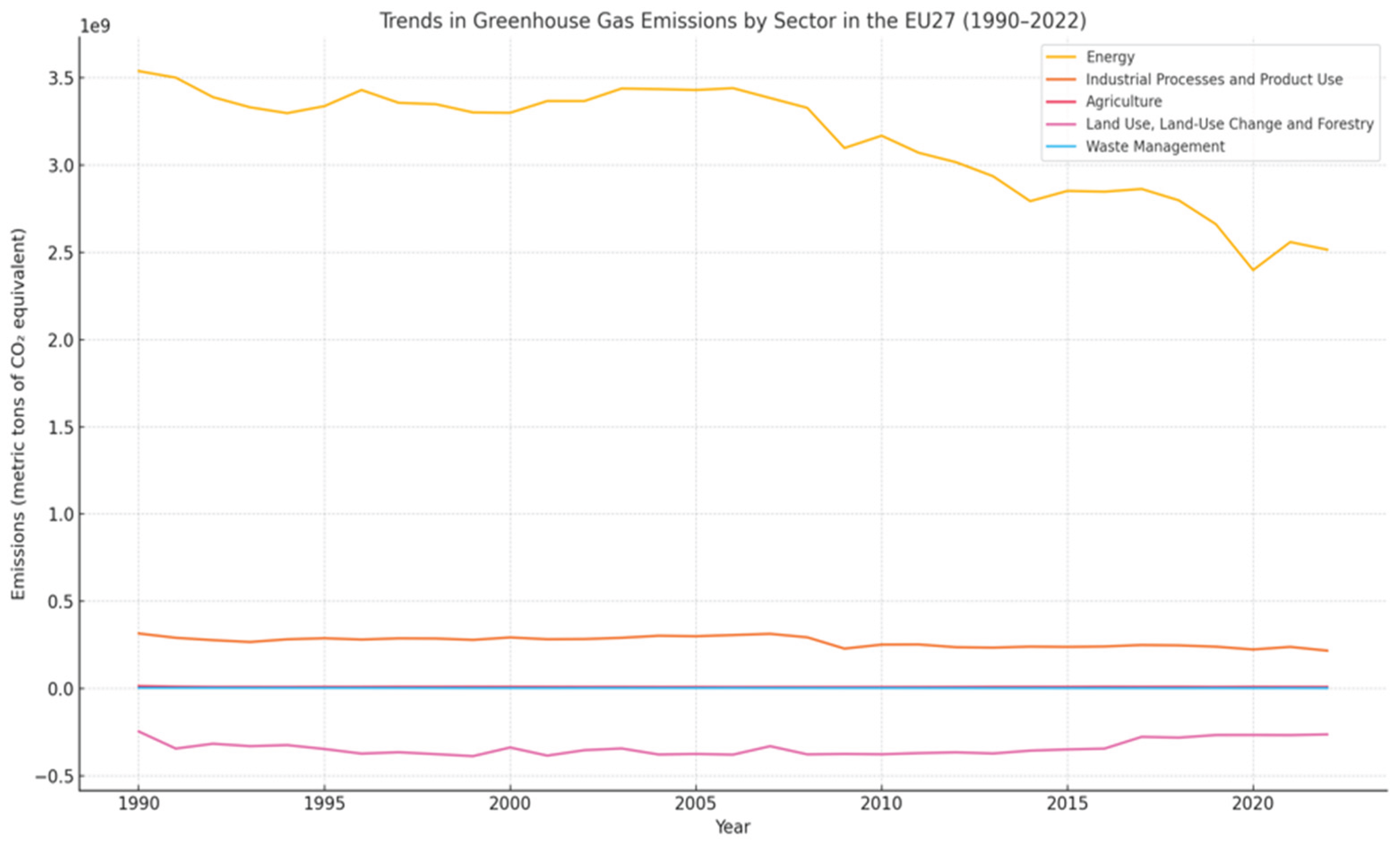
Figure 2.
Total Greenhouse Gas Emissions in the EU27 Excluding LULUCF (1990–2022).

Figure 3.
Sectoral Composition of Greenhouse Gas Emissions in the EU27 (Excl. LULUCF), 1990–2022.
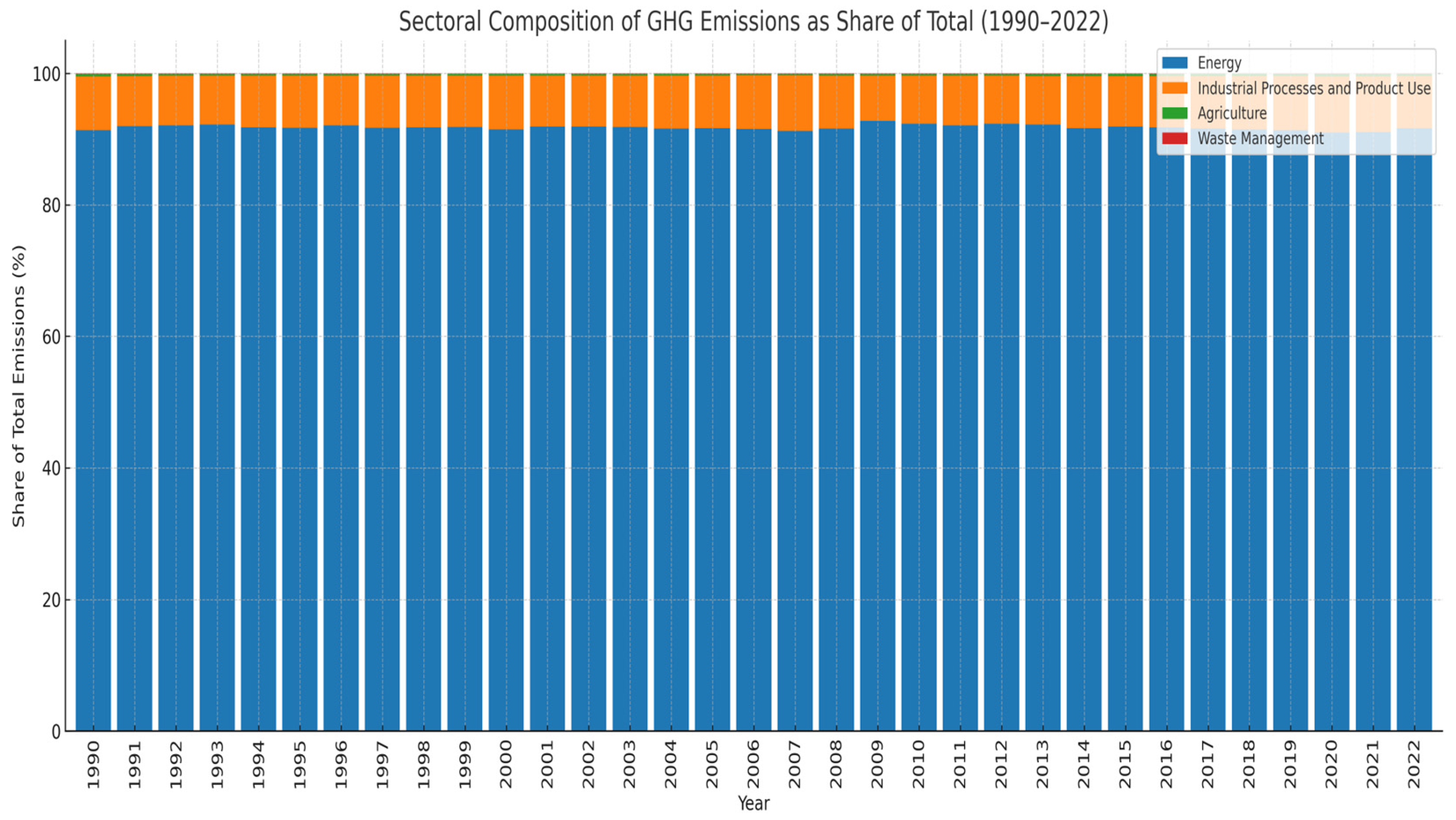
Figure 4.
Year-over-Year Change in Total GHG Emissions in the EU27 (Excl. LULUCF), 1991–2022.
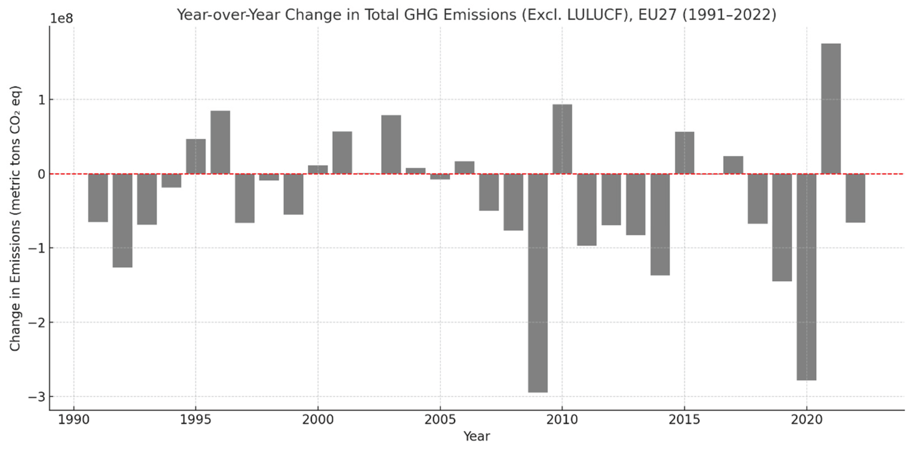
Figure 5.
Inter-Sectoral Correlation Matrix of GHG Emissions in the EU27 (1990–2022).
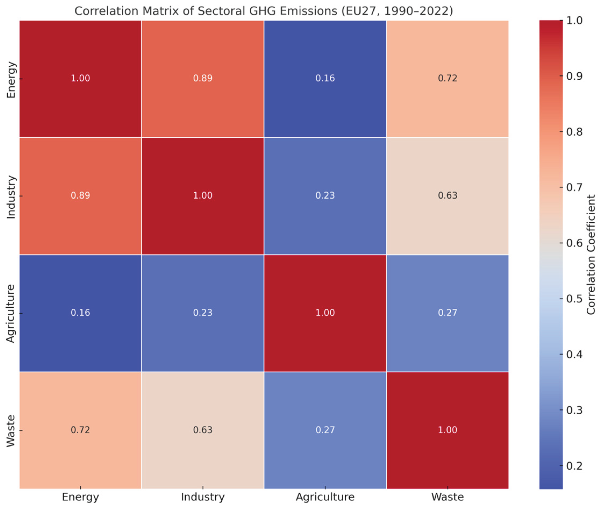
Figure 6.
Autocorrelation Function (ACF) of Total GHG Emissions (EU27, 1990–2022).
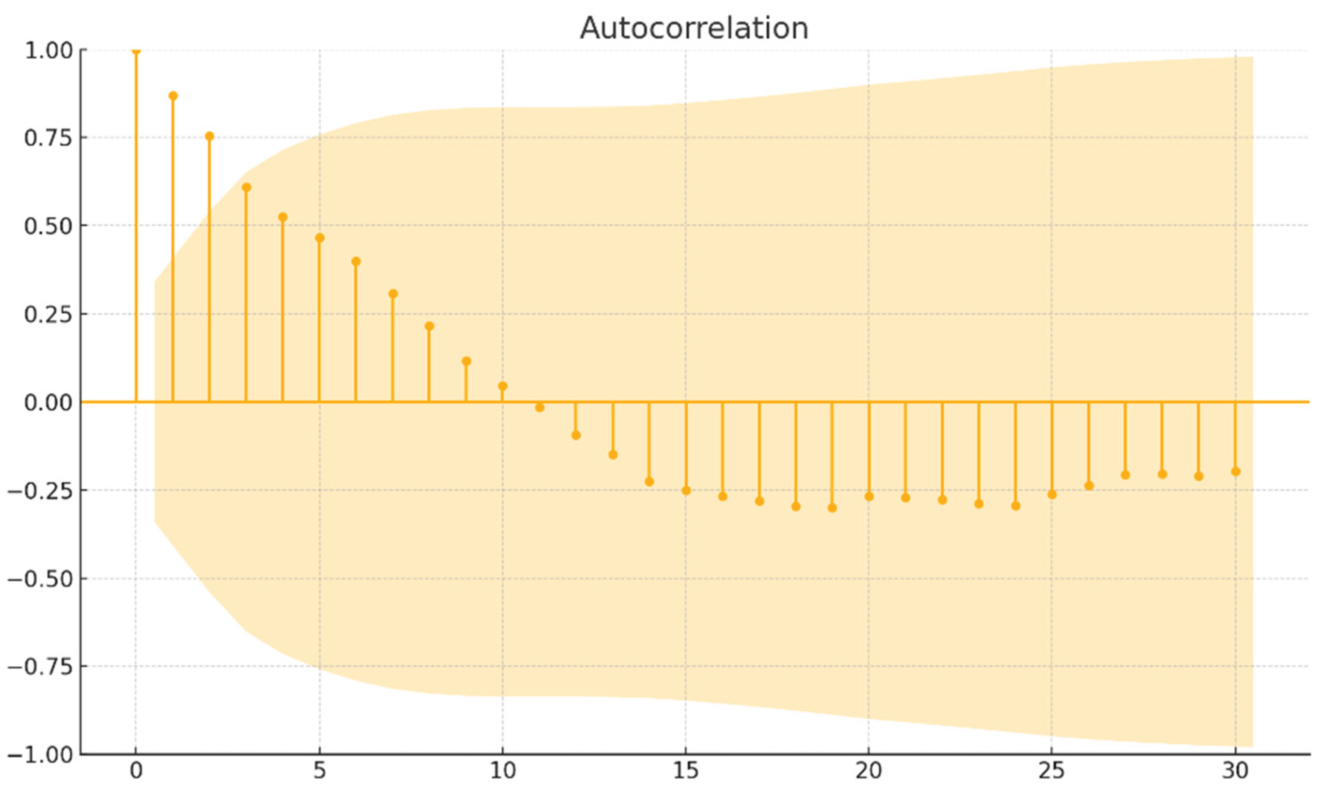
Figure 7.
Partial Autocorrelation Function (PACF) of Total GHG Emissions (EU27, 1990–2022).
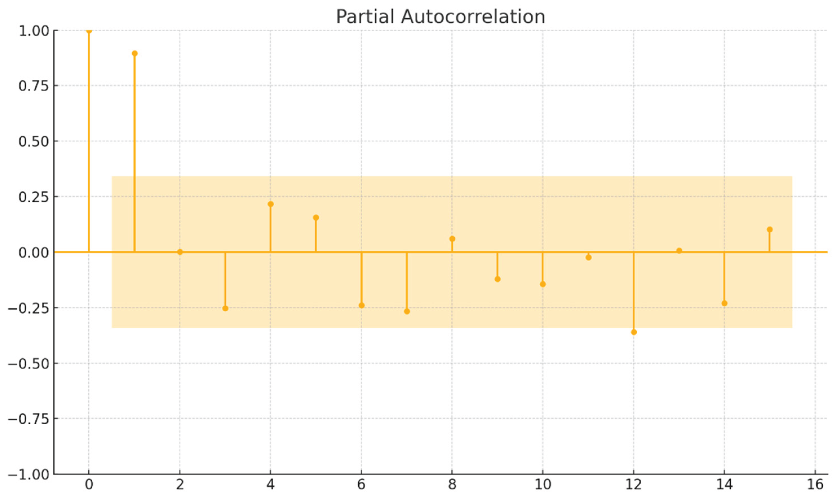
Figure 8.
ARIMA-Based Forecast of Total GHG Emissions in the EU27 (Excl. LULUCF), 2023–2030.
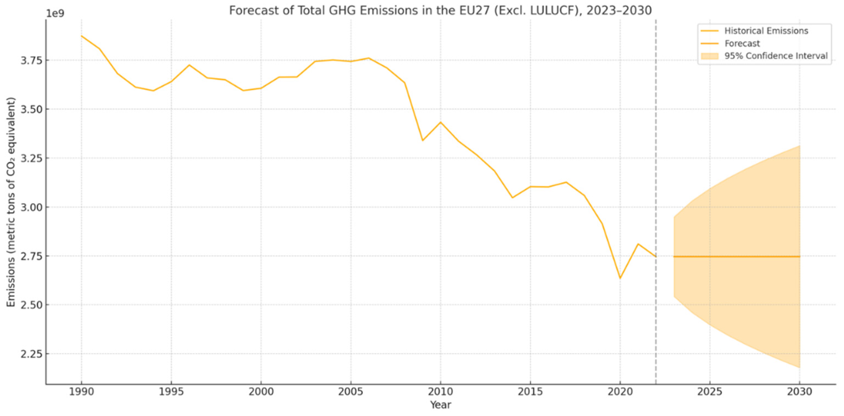
Figure 9.
Hybrid Forecast Output: ARIMA + Random Forest (2023–2030).
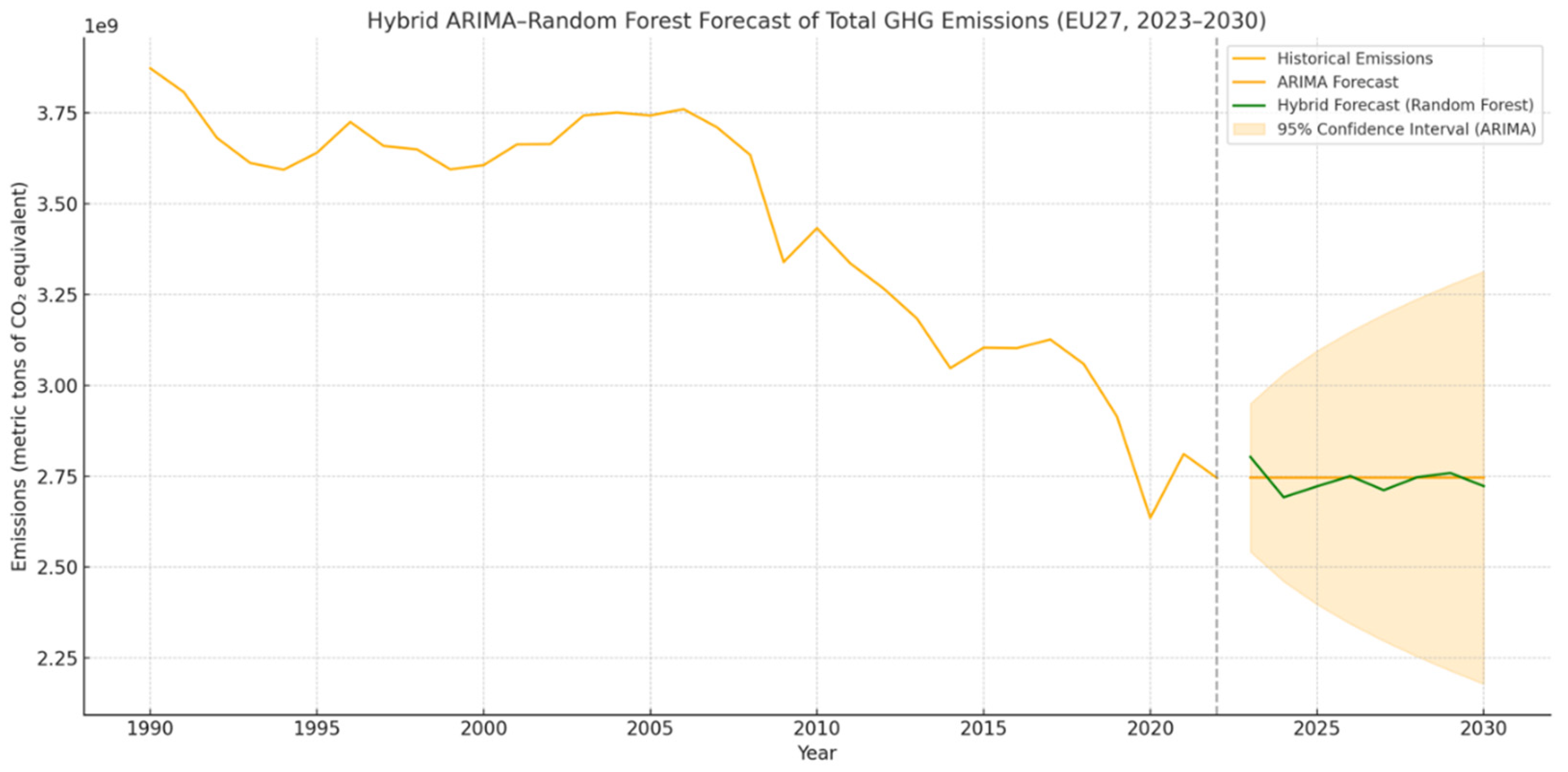
Figure 10.
Smoothed Regime Probabilities – Markov Switching Model.
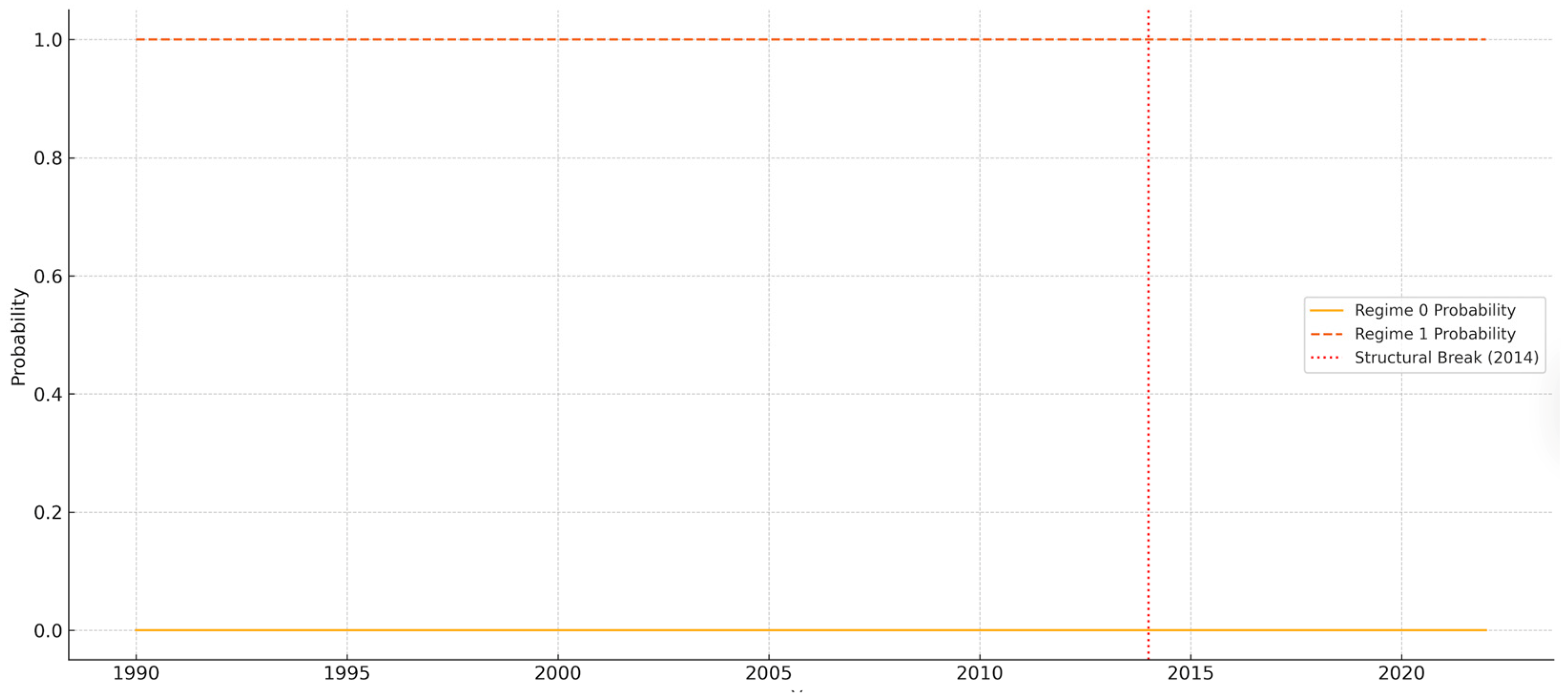
Figure 11.
Segmented Linear Fit with 95% Confidence Intervals.
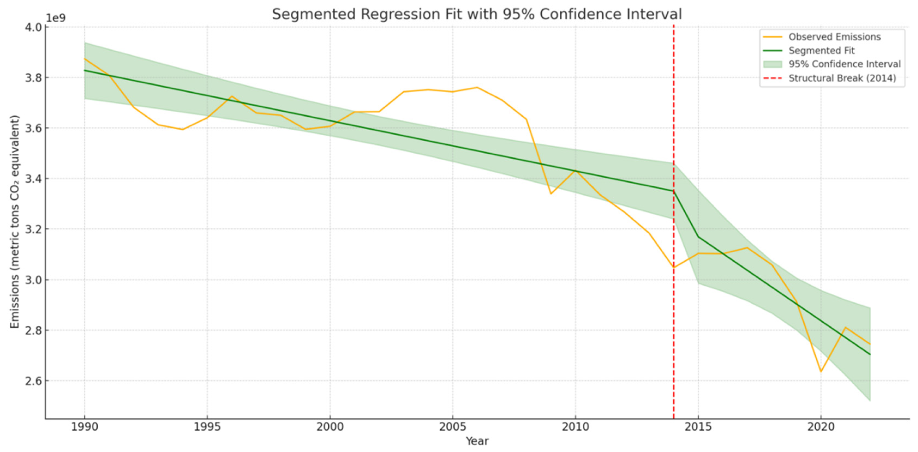
Figure 12.
Emissions Pathways Under Three Policy Scenarios to 2030.
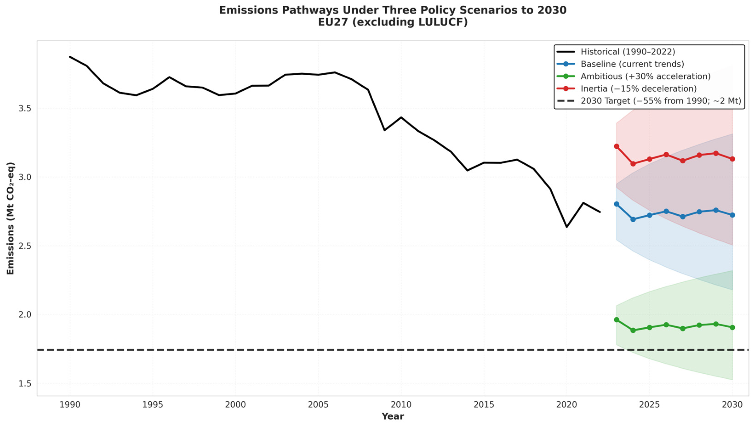
Figure 13.
Comparative Modelling of EU27 GHG Emissions — Linear, Segmented, and Hybrid Forecasts (1990–2030).
Figure 13.
Comparative Modelling of EU27 GHG Emissions — Linear, Segmented, and Hybrid Forecasts (1990–2030).
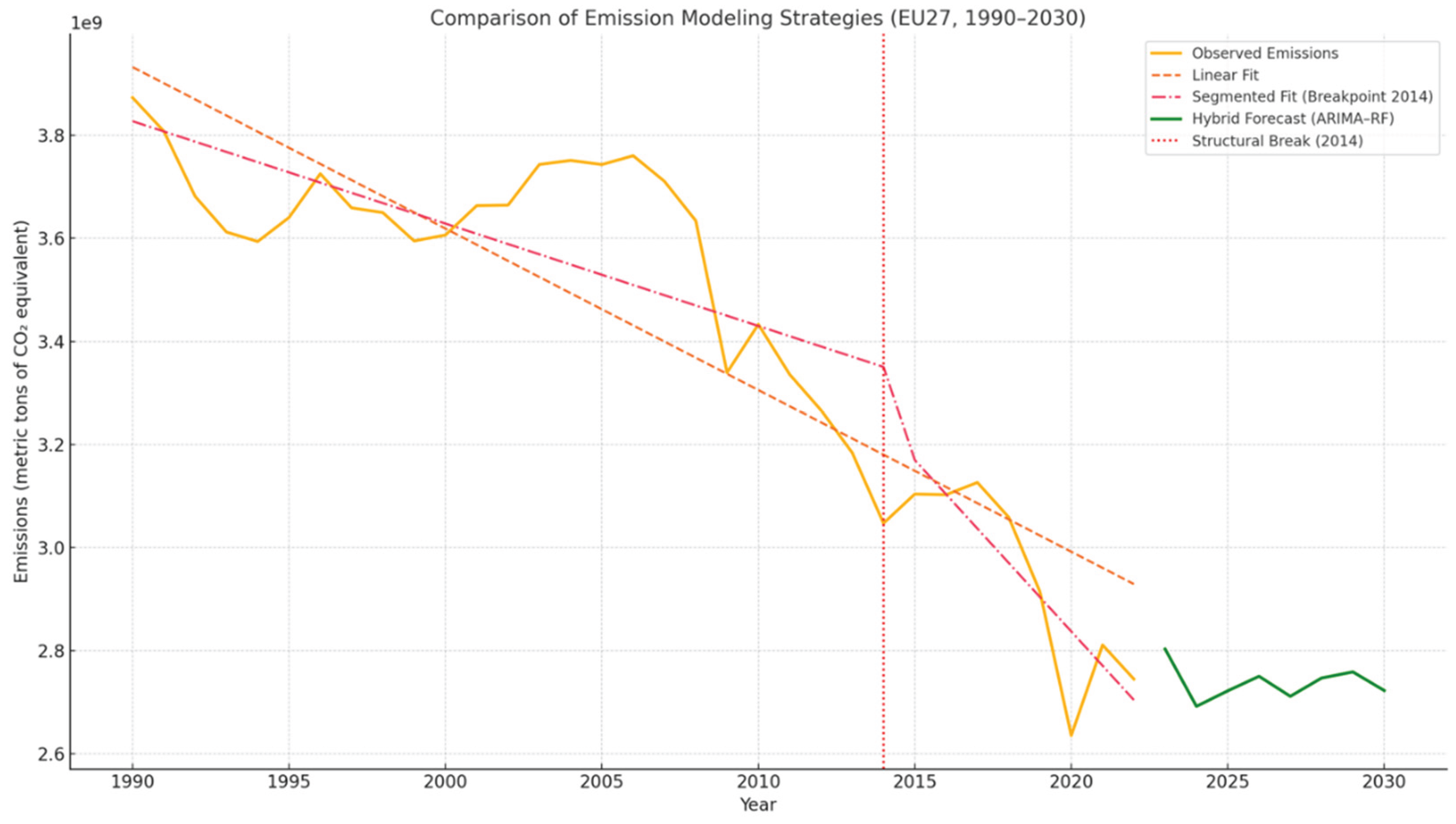

Table 1.
Hyperparameters and Validation Metrics of the Hybrid ARIMA-RF Model.
| Component | Parameter | Value / Specification |
|---|---|---|
| ARIMA | Order (p,d,q) AIC AIC improvement AR coefficient φ₁ |
(1, 1, 0) 425.32 ΔAICc = 8.85 vs (0,1,0) 0.641 |
| Random Forest Hyperparameters |
n_estimators max_depth min_samples_split min_samples_leaf criterion |
100 10 5 2 2 |
| Training Data | Lag order (n_lags) Training observations Feature matrix shape |
5 27 27 × 5 |
| Cross-Validation (5-fold) |
Method R² (mean ± std) MAE (mean ± std) RMSE (mean ± std) |
5-fold CV 0.52 ± 0.08 35.4 ± 7.2 Mt CO₂-eq 47.3 ± 9.1 Mt CO₂-eq |
| Bootstrap CI | Iterations Percentiles (α=0.05) Resampling method |
1,000 [2.5%, 97.5%] With replacement |
Note: All metrics computed on EU27 emissions data (1990–2022). CV = cross-validation; CI = confidence interval.
Table 2.
Scenario Projections for EU27 Emissions in 2030.
| Scenario | Description | 2030 Projection | 95% CI Lower | 95% CI Upper | Annual Reduction Rate Post-2022 | Gap to Target |
|---|---|---|---|---|---|---|
| Baseline | Current policy trends; no acceleration | 2,746 Mt | 2,609 Mt | 2,883 Mt | −2.1% | +1,003 Mt |
| Ambitious | +30% acceleration; intensified policy | 2,244 Mt | 2,087 Mt | 2,401 Mt | −2.8% | +501 Mt |
| Inertia | −15% deceleration; implementation gaps | 3,047 Mt | 2,864 Mt | 3,230 Mt | −1.4% | +1,304 Mt |
| 2030 Target (Fit for 55) | −55% from 1990 baseline | ~1,743 Mt | — | — | −3.2% (minimum) | — |
Note: All projections in Mt CO₂-eq. EU27 excluding LULUCF. Target represents a 55% reduction from the 1990 baseline (Fit for 55 package). CI = confidence interval computed via bootstrap resampling (n = 1,000 iterations). The gap to Target shows the difference between the scenario projection and the legally binding 2030 target.
Table 3.
Stationarity Testing Summary (ADF Tests).
| Series | ADF Statistic | p-value | Type |
|---|---|---|---|
| Original Series | -2.3539 | 0.1596 | Non-stationary |
| Differenced Series | -5.6542 | 0.0000 | Stationary |
Disclaimer/Publisher’s Note: The statements, opinions and data contained in all publications are solely those of the individual author(s) and contributor(s) and not of MDPI and/or the editor(s). MDPI and/or the editor(s) disclaim responsibility for any injury to people or property resulting from any ideas, methods, instructions or products referred to in the content. |
© 2025 by the authors. Licensee MDPI, Basel, Switzerland. This article is an open access article distributed under the terms and conditions of the Creative Commons Attribution (CC BY) license (http://creativecommons.org/licenses/by/4.0/).
Copyright: This open access article is published under a Creative Commons CC BY 4.0 license, which permit the free download, distribution, and reuse, provided that the author and preprint are cited in any reuse.


