
Submitted:
09 November 2025
Posted:
10 November 2025
You are already at the latest version
Abstract
Long-term monitoring of radon (222Rn) and thoron (220Rn) radioactive gases has been used in earthquake forecasting. Seismic activity before earthquakes raise the levels of these gases, causing abnormalities in the baseline values of Radon and Thoron Time Series (RTTS) data. This study reports applications of Kernel Density Estimation (KDE) and Wavelet-Based Density Estimation (WBDE) to detect anomalies in radon, thoron, and meteorological time-series data. Anomalies appearing in the RTTS data have been assessed for their potential correlation with seismic events. Using KDE and WBDE, radon anomalies were observed on March 12, August 15, September 17, in the year 2017, and January 19, 2018. Thoron anomalies were recorded on March 12, August 15, September 17, 2017, and February 28, 2018. Irregularities in RTTS were observed several days before seismic events. Anomalies in RTTS, detected using KDE, successfully correlated five out of nine seismic events while WBDE identified four anomalies in RTTS which were successfully correlated with the corresponding seismic events. The wavelet transform has been used to reduce noise at higher decomposition levels in radon and thoron time series. Findings of the study reveal the potential of radon and thoron time series that can be used as precursors for earthquake forecasting.
Keywords:
anomaly detection
; radon
; thoron
; seismic events
; kernel density estimation
; radioactivity
1. Introduction
Many studies in the literature have recognized radon as a potential earthquake precursor. Scientists have studied radon extensively in the context of seismic forecasting. Various other techniques can be found in the literature for earthquake forecasting, such as, abnormal animal behavior [1], unusual geochemical activity [2], variations in seismic wave velocity [3,4] and alterations of several types of electromagnetic precursors e.g. see reviews [5,6]. Radon emission and monitoring have remained a popular technique in earthquake forecasting studies [5,6,7,8,9] and is considered among the precursors with the general model of Lithosphere Atmosphere Ionosphere Coupling (LAIC) e.g. see review [10]. Beside various studies reporting health impacts of elevated levels of radon and thoron e.g., reports in [11], many studies have reported that anomalous fluctuations in radon time-series data have been linked with seismic activity; however, these variations may also stem from additional factors, such as soil porosity, radionuclide composition, lithological characteristics, and meteorological influences, including rainfall, humidity, atmospheric pressure, and temperature [13,14]. Filtering out the effects of these perplexing factors, radon anomalies can serve as a reliable indicator for forecasting impending earthquakes.
Radon time series is analyzed for identification of anomalies within the dataset in order to get a better understanding of variations in radon and thoron concentrations and to establish a possible link between anomalies and forecasting of impending earthquakes e.g. see reviews [5,6,10]. It is very important to explore factors that cause changes in RTTS in order to find a link between these changes and seismic activity. Anomalies in RTTS may arise due to geophysical phenomena and environmental factors. Over the years, many advancements have been witnessed in refining existing and proposing new methods for the detection of anomalies in RTTS. Towards this, investigators have tried to account for large data volumes and the dynamic variability in data patterns. For complex dynamical systems, there is always a need to develop more advanced and intelligent-based anomaly detection techniques to address complicated processes that cause these anomalies [14].
Based upon specific applications, scientists have developed several algorithms, with certain advantages and disadvantages, to detect anomalies in time series. Some of the widely used methods to detect anomalies are clustering based approaches, Bayesian online change point detection (BOCD), auto-encoders, Statistical Process Control (SPC), moving average, seasonal decomposition of time series, Delegated Regressor Method [15] and Autoregressive Integrated Moving Average (ARIMA).
In the present study, anomaly in RTTS data was identified using Kernel Density Estimation (KDE) technique by evaluating the probability density function for the normal data points. The technique rests on the foundation that data points deviating significantly from the distribution are taken as anomaly. The non-parametric nature of KDE technique make it a good choice to detect anomaly. An additional advantage of KDE is that it generates density plot that display a clear graphical representation of data points thereby identifying potential outliers in original time series. KDE has ability to handle complex patterns and abrupt changes in time series making it a robust method for anomaly detection [16].
Kernel density estimation detects anomalies by estimating probability density function (PDE). It is also referred as Parzen’s window [17]. Kernel density estimation automatically estimates density of of the given dataset through automatic data processing. Laxhammar et al. [18] have proposed a Gaussian mixture model (GMM) and adaptive Kernel Density Estimator (KDE) for the purpose of anomaly detection. KDE characterizes the normal data accurately through examining the normality modeling. Anomaly detection results using these two methods shows there is no big difference between these two methods. Moreover, the performance of both approaches is deemed to be suboptimal.
Ramanna et al. [19] proposed a zone-free approach for better identification of areas with diffused and spread seismicity. This zone-free approach used the adaptive kernel density estimation (KDE) technique. The main merit behind the adaptive kernel technique outperforms the fixed kernel technique statistically is that the bandwidth of the kernel is spatially variable. This is based on how sparse or clustered the epicenters are. The fixed kernel approach performs poorly with multimodal and long-tail distributions, despite its general success in density estimation scenarios. Because the activity rate probability density surface is multimodal in nature, the adaptive kernel technique is useful in these circumstances and more pertinent to earthquake engineering.
Zhang et al. [20] provided a density-based, unsupervised method for anomaly detection, determining a smooth and efficient anomaly detection method that can be applied to non-linear systems. They used the Gaussian kernel function to attain smoothness in the data. Additionally, adaptive kernel width is used to improve the discriminating power of the model. In high density regions, wide kernel widths are applied to smooth out the difference between normal samples, and in low-density regions, narrow kernel widths are applied to emphasize the abnormality of potentially anomalous samples
In order to mitigate noise from the input signal, Kordestani et al. [21] tested and presented a wavelet-based approach. A finite number of independent observations is used to estimate probability densities using a technique called wavelet-based density estimation (WBDE). It is not necessary to choose a global smoothing scale in advance, and the suggested method can adapt locally to the smoothness of the density depending on the provided discrete particle data. It also maintains the moments of the particle distribution function with a high degree of accuracy and has no restrictions on the system's dimensionality.
García-Treviño and Barria [22] have proposed online wavelet-based density estimation for non-stationary, rapidly changing streaming data (e.g., sensor data, computer network traffic, ATM transactions, web searches). Their methodology was constructed on a recursive formulation of the wavelet–based orthogonal estimator using a sliding window. Computer experimentation demonstrates that their proposed method works well, involving cases for non-stationary applications where the corresponding probability density function is changing with respect to time, and it also works for cases involving running average-based metrics. They have tested their algorithm for simulated and real-world environments and found that their proposed method with good adaptation capabilities that require a fixed amount of memory
In the current study, Kernel Density Estimation (KDE) was used to detect anomalies in radon and thoron time series data. Histogram-based Density Estimation (HBDE) was also employed. Wavelet-based decomposition was applied to the same dataset to discriminate between noise and denoised signals. Following the decomposition, wavelet-based density estimation (WBDE) was performed. The resulting densities were analyzed in relation to identified anomalies. The study spanned over a period of one year, collecting extensive data to support the analysis. This paper also demonstrates the potential of KDE for reliable anomaly detection in environmental radioactivity monitoring.
2. Materials and Methods
This section first presents the instrumental aspect, namely, the underlying geology, the monitoring apparatus and the related earthquake data. Then, the theoretical aspects are described namely the background of the KDE and WBDE methods. As aforementioned both methods are employed for detecting anomalies in radon and thoron time series. The main objective is to investigate the use of KDE and WBDE to identify patterns and anomalies that precede seismic activity. As will be presented both methods are promising and not extensively used in this specific subject. Moreover. as successful anomaly detection via KDE and WBDE will enhance our tools in forecasting earthquakes. The employed dataset spans over a year, comprising radon, thoron, and meteorological data, while nine earthquakes are included the study.
In the following subsections these will be presented in detail.
2.1. Instrumental Aspects
2.1.1. Geology of the Study Area
The data of the current study has been recorded in Muzaffarabad, the capital of the Pakistan-administered state of the Azad Jammu and Kashmir. Muzaffarabad is located at atitude 34.37002° and longitude 73.47082° at the confluence of two rivers, Neelum and Jhelum. The regional tectonic map of the westernmost part of the frontal Himalaya is shown in Figure 1.
Muzaffarabad district covers a total area of 1,642 km², while Muzaffarabad city itself spans approximately 17 km² [23]. Tectonically, Muzaffarabad is situated within the Hazara-Kashmir Syntaxis (HKS), a geologically significant and seismically active structure located in the western Himalayas. The HKS is formed by the folding of Himalayan thrust sheets in the northeastern region of Pakistan [24]. Several active faults are associated with the eastern limb of the HKS, including the Muzaffarabad Fault (MF), Riasi Fault (RF), Shahdara Fault (SF), Shaheed Gala Fault (SGF), Godri Badshah-Kotli Fault (GK), Pirgali Fault (PF), and Samwal Fault (SF).
The Muzaffarabad Fault is also known as Himalayan Frontal Thrust (HFT), Tanda Fault (TF) and Balakot-Bagh Fault (BBF) [25]. The Muzaffarabad Fault creates the massive active rupture zone, which ranged from one to three kilometers. Landslides, gouges, fractures, and cracks are all common in this rupture zone. The morphology along Muzaffarabad Fault is governed by warps or folded scarps, fault-related fold scarps. The local pop-ups, triangular zones, pressure ridges, and stretching movements are evident across this fault.
The Muzaffarabad Fault was recognized to be active prior to the devastating earthquake that struck on October 8, 2005, with the magnitude of Mw=7.6, which occurred at 8:52 am PST (3:50:40 UTC). The epicenter for this earthquake was situated 18 kilometers north-northeast of Muzaffarabad, the capital of Azad Jammu and Kashmir, with a focal depth of 26 km [27].
2.1.2. Data Acquisition
The radon and thoron radioactive gases were measured using the SARAD RTM 1688-2 active radon thoron monitor [28]. By using the above active monitor, soil radon, soil thoron, and the meteorological parameters temperature, pressure, and humidity, have been continuously monitored from March 2017 up to May 2018. To install the RTM 1688-2 for in-situ measurements, a borehole 1 m deep from the soil’s surface was dug. There, the packer probe of RTM 1688-2 was brought down, properly sealed from the surrounding air so that the pumped gas to be only from the nearby soil. Measuring period was 40 min. In this manner, RTM 1688-2 collected 36 samples per day yielding to a total of 15692 data samples were taken during the study period.
2.1.3. Earthquake Related Data
The earthquake data was obtained from the National Seismic Monitoring Centre of Pakistan [29] and refer to the parallel period of measurements Section 2.1.2 plus-minus one month to allow for pre- and post-earthquake data. In oder to select earthquakes from this period, the earthquake preparation radius of Dobrovolsky et al. [30] was calculated:
The rear should not that equation (1) is still in extensive use in the related literature. The hypothesis in [30] is that, prior to seismic events, a circle of radius exists around the epicenter, within which, major elastic crustal deformation occurs. In this consensus, it is essential that radon and thoron monitoring stations are installed within the radius in order to ensure (according to [30]) that the station’s measurements are influenced mainly by the seismic activity. This means that to account for (mainly) seismic activity, the distance of the radon-thoron measurement station from the earthquake epicenter must be within the earthquake preparation radius, namely the Dobrovolsky’s radius must greater than the epicentral one, i.e., ≥. Under this criterion, nine earthquakes are identified during the earthquakes’ period. These earthquakes are presented in Table 1 together with the Dobrovolky’s and epenentral radii.
2.2. Theoretical Aspects
2.2.1. Kernel Density Estimation
KDE has been introduced in statistical and geostatistical studies, however nowadays is utilised in physics, public health, astronomy, agriculture, social economy [31] and seismic research [32]. It is considered among most popular non-parametric techniques for the estimation of the of probability density function (PDF) of a time series or a variable of a dataset. According to Zhang et al. [20] KDE can be used in anomaly detection in non-linear systems by detecting the density variations in KDE heatmap, which visualize these anomalies A low probability density in the KDE heatmap is associated with an anomaly in the data series [20].
Mathematical expression for the kernel density can be estimated by considering it as a matrix of identically distributed samples. These samples are taken from a probability kernel density,, from the m-dimensional Euclidean space given as [18]:
KDE has been employed in detection of anomalies in time series. This is because it offers a nuanced understanding of the anomaly detection by encoding, decoding and evaluating post-training, events against the estimated density, providing hence a comprehensive notion of normality [34]. This is achieved by comparing the density of each sample with the one neighborhood through calculation of the average density of all nearby samples [35]. Anomaly detection via KDE can be accessed in geochemistry [36], pattern recognition [37], droughts [38], magnetic fields [39] and other disciplines.
2.2.2. Histogram-Based Density Estimation
Estimating the densities of any time series data can be also carried out using histogram-based density estimation. It can be easily set and its implementation is of low complexity in time. HBDE distribution density, being discontinuous, restrict it to be good choice for the purpose of anomaly detection [35]. However, HBDE can be effectively used for estimating distribution of data when the actual distribution is not known. Estimated density due to HBDE technique is sensitive to the choice of bin width. While considering limitations of histogram-based density estimation technique, other density estimation models are used for the detection of anomalies.
2.2.3. Wavelet-Based Density Estimation
Wavelets are common mathematical tools used for the analysis and computation of non-stationary time series. Wavelets can be locally adjusted so as to follow the smoothness of any function due to their multi-scale nature [40]. Due to this fundamental characteristic, wavelets have been used in a variety of applications. Their most important application is the denoising of non-stationary signals [41]. The key achievement of wavelet thresholding to reduce noise depends upon the fact that the extension of input signals in a wavelet basis is usually sparse, i.e.,several features of the input signal are effectively summarized by a small fraction of wavelet coefficients [40,412].
Wavelet-based density estimators are actually orthogonal series estimators, that is a broad family of non-parametric techniques [42]. The two most widely used orthogonal series are the Fourier and Hermite functions. In comparison to other orthogonal functions for WBDE, the above functions provide greater flexibility in smoothness and convergence [22]. Initially, in. the so called, conventional wavelet density estimation only the preliminary density was approximated. With the evolution of the knowledge in the field, a recursive data modification was achieved which takes into account the data in calculations and also the exponential depreciation of previous data. Through this updating process the coefficients in orthogonal series estimators are represented by the expected value of each data point is projected across the orthogonal series [43].
Wavelet based estimators have not been employed extensively so far and, as a result, the related papers are scarce during the last decade. Jiang et al. [38] employed also wavelet based estimators for droughts.WBDE has been utilised to estimate the uncertainty and bias of hydro-climatological changes [44], to quantify anomalies for Mobile Information Carriers [45] and to study precipitation extremes and large scale climate anomalies [46].
3. Results and Discussion
Time series data of radon, thoron, temperature, pressure, and humidity parameters have been collected continuously for 436 days. According to the in situ experience and the publications of the team [e.g references in 15 and 41], this time period is adequate for the study of radon and thoron disturbances in association with earthquakes. Table 2 shows the values from the KDE and WBDE methods applied to the radon and thorοn time series during period of study. It can be observed that values of the RTS of the earthquakes 6 and 9 tend to be higher than the values for the other earthquakes. WBDE has a tendency to higher value only for earthquake 6. KDE values for TTS tend to be higher for earthquakes 4 and 5, while from WBDE for earthquake 1 and 2. This differentiation can be attributed to a different sensitivity of each method in respect to the time series and earthquake occurrence. To study the density value tendencies further, the average density values are calculated and then the cut-off limit of average+2standard deviation is arbitrary set. The reasoning is that the density values that are above the cut-off limits are unusually high. These cut-off points are given in the last row of Table 2. Only the densities of the radon time series of earthquake 9 from KDE values and of earthquake 7 from the WBDE values are increased. It is obvious that the pure density values of Table 2 provide non-systematic pre-earthquake estimations and therefore the values are only indicative.
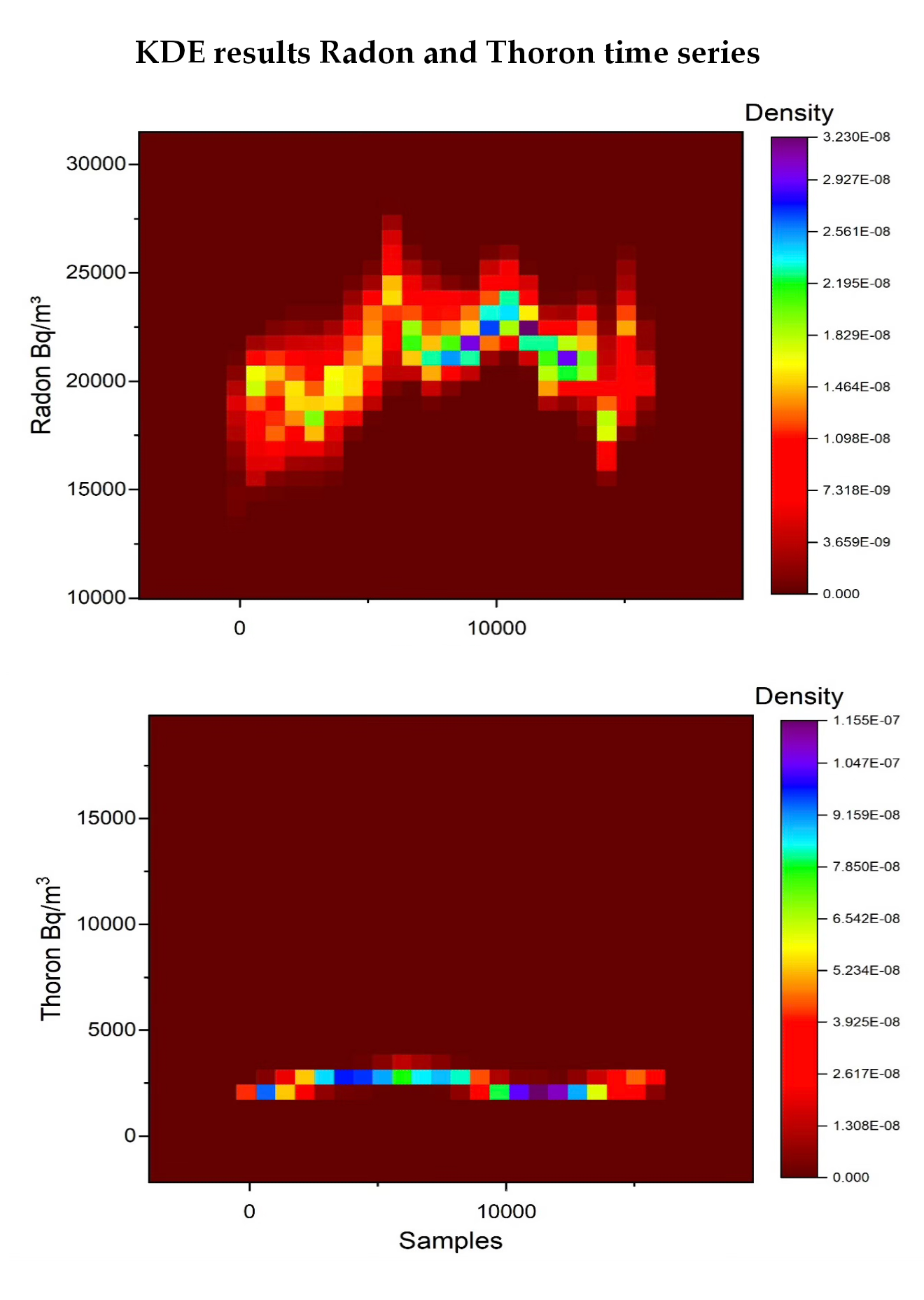
It is obvious fro the above viewpoint, that other types of calculations can be advantageous in analysing the radon and thoron data in relation the the studied earthquakes. Towards this the time evolution of the KDE heat map could provide adequate information (Figure 2, Figure 3, Figure 4, Figure 5 and Figure 6). The reader should note here that according to the colour bar of each Figure 2, Figure 3, Figure 4, Figure 5 and Figure 6, where the density is high, hot colors occur, such as reds and yellows. Taking into account the colour bar values. High density corresponds to profile values, i.e. baseline levels, whereas low density localities are associated to anomalous values and cooler colours such as blues or greens. Finally, time intervals with a significant lack of color or very low density are associated with unusual or irregular measurements.
Under the above consensus, radon (Figure 2), thoron (Figure 3) and atmospheric (Figure 4, Figure 5 and Figure 6) time series shows unusual KDE density values at certain time samples. To interpret the time axis, the reader may recall form Section 2.1.2 that each sample correspond to a 40 min measuring interval. In this view, radon time series show anomalous KDE densities on 12 March 2017 i.e. 11 days prior to the occurrence of the MW=4.3 (21 March 2017, EQ1) earthquake and 13 days prior to the MW=2.5 (23 March 2017, EQ2) earthquake. The radon also shows anomalous kernel density in density on 15 August 2017, i.e., 12 days before the occurrence of earthquakes of magnitude MW=4.8 (27 August 2017, EQ3). The anomaly in KDE density was also observed in radon on 17 September 2017, i.e., 7 days before the occurrence of earthquakes of magnitude MW=4.6 (23 September 2017- EQ4). Another KDE density anomaly was observed in radon time series on 19 January 2018, i.e., 15 days before the occurrence of earthquakes of magnitude MW=0.8 (3 February 2018.EQ6). The reader should however note here that the above results are valid in the logic of what KDE heat map provides. The corresponding evidence hence are valid under these constrains and they may be subjected to methodology bias if different mathematical approaches are selected.
Thoron also shows anomalous nature in density (Figure 3) on 17 August 15 2017, i.e., 12 days prior to the occurrence of earthquakes of magnitude MW=4.8 (27 August 27 2017, EQ3). KDE density density was also observed in thoron on 17 September 2017, i.e., 7 days before the occurrence of earthquakes of magnitude MW=4.6 (23 September 23 2017, EQ4). Another KDE density anomaly was also observed in thoron on 28 February 2018, i.e., 15 days before the occurrence of earthquake of magnitude MW=0.8 (03 February 2018, EQ6).
From the results presented so far, it is evident that the KDE method manages to identify anomalies in radon and thoron time series in link with the earthquakes of Table 1. This gain of KDE is noteworthy especially if the reader accounts that according to Frehner at el. [34] Among the techniques specifically developed for anomaly detection, there is no clear winner. It is evident from the recent review of Nikolopoulos et al. [5] on earthquake precursors, that there is no single certain rule to link earthquakes and anomalies but several papers report such links for even mild earthquakes. In the sense of this review, the present results fall within the tendencies of both recent and old papers. Moreover, the recent review of Pulinets et al. [10] the Lithosphere Atmosphere Ionosphere Coupling (LAIC) adopts anomalies from all the parts. The reader should note that the first author of reference [10] is the maim founder of the LAIC model which is used extensively nowadays for the explanation of pre-earthquake anomalies. The present results referring on anomalies from data in soil, i.e., from the lithosphere, is both within the LAIC model and the international literature. The review of Conti et al. [6] also verifies this aspect. Hence it can be supported that both radon and thoron anomalies identified through KDE are supported by evidence. Moreover, the fact that KDE has been applied to several types of anomalies (see references of Section 2.2.1), it is also evident that this method is indeed robust, modern and succeeds in delineating anomalies. The method managed to identify five from the nine earthquakes of Table 1.
Since KDE method is successful in finding radon and thoron anomalies as well as time series anomalies in general, it may be used also for the delineation of anomalies of the atmospheric parameters related to radon and thoron data series. According to this sense, Figure 4, Figure 5 and Figure 6 present the variations of the atmospheric parameters with the KDE method. The reader should note here, that traditionally, radon and thoron series are presented in parallel to atmospheric data series. This is because the atmospheric parameters may evoke anomalies in radon and thoron due to the physics of the lithosphere (underlying geology). Classical papers explain that and the reader may find several such references in the references of the reviews [5,6,10]. It should be noted though, that this is a not necessary condition, meaning that it is not obligatory or priory that some kind radon or thoron anomaly is due to atmospheric parameters disturbances. That further means, that even if some indications may co-exist with atmospheric parameters and radon or thoron anomalies, it is not obligatory to associate the disturbances to variations of the atmospheric parameters ad not to seismic events. After these evidence, the reader may observe that the KDE heat map of the atmospheric parameters id not identical to the one for radon and is completely different from the one of thoron time series. In an alternate interpretation, radon time series may has KDE heat maps of all atmospheric series and no single one. On the contrary, thoron time series has no related heat map. According to this consensus, the claims presented regarding the potential links on the earthquakes of Table 1 and radon time series are valid whereas the claims from thoron time series are more strict. The link between the earthquakes of Table 1 and the radon and thoron time series, is reinforced by the findings of the HBDE method (Figure 7, Figure 8, Figure 9, Figure 10 and Figure 11).
Indeed the HBDE estimation of radon time series are very different from the ones of temperature (Figure 9) and relative humidity (Figure 10). The HBDE of air pressure time series (as with the KDE heat maps) have some similarities with the radon time series implying also a bias due to atmospheric pressure in radon time series. Regarding thoron time series there is again no similarities. Therefore tit can be supported that thoron time series manage to delineate better the link to earthquakes of Table 1, but the claims for the links with radon time series are also valid.
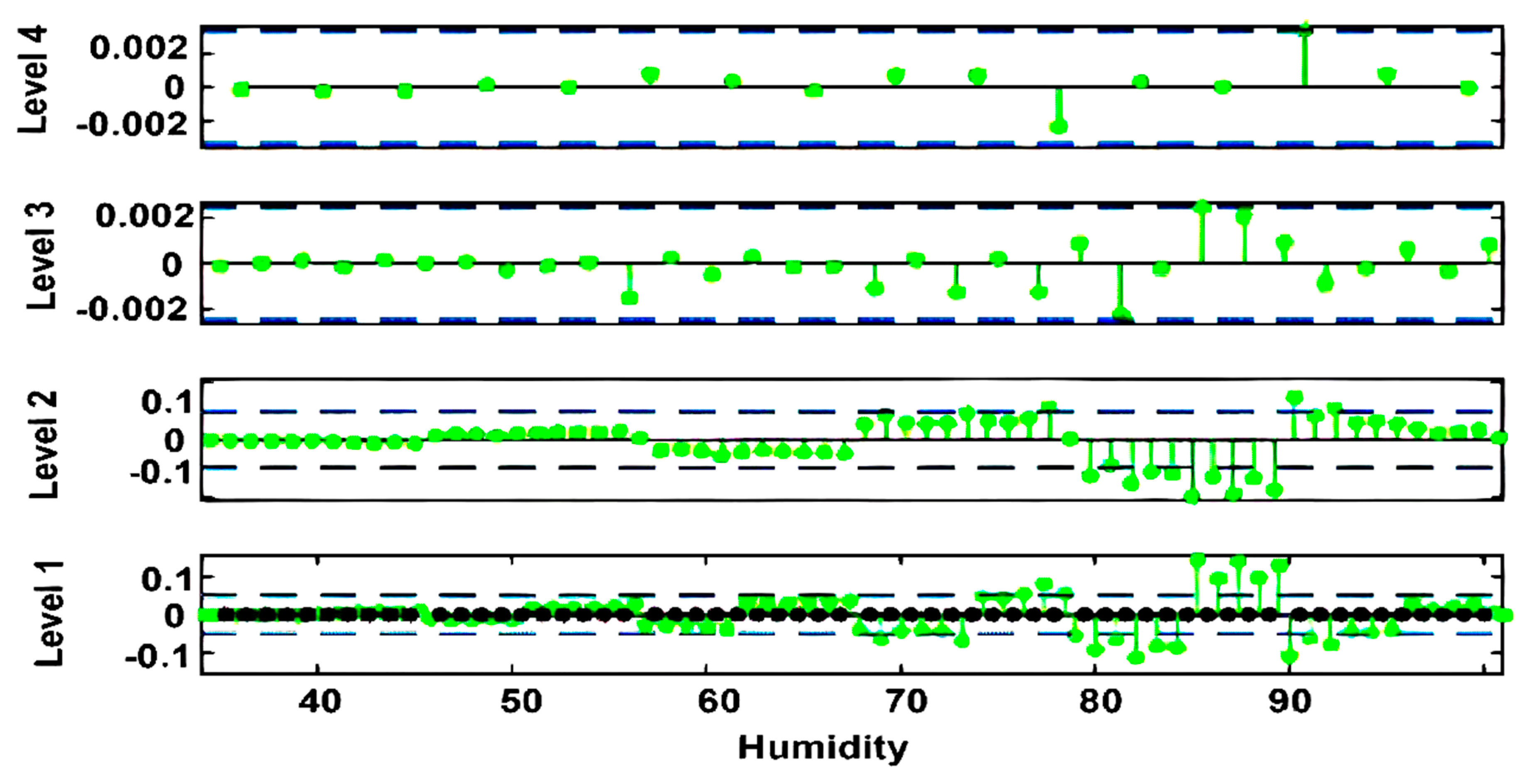
Figure 12 through Figure 16 present the wavelet coefficients of radon, thoron, and meteorological time series using the Bior (Biorthogonal) wavelet. The reader should note here that the black or coloured spots indicate wavelet coefficients with higher amplitudes. These spots may represent the important information in the data at the various scales and locations. Black dots may indicate strong coefficients, making them more prominent. A black spot in the wavelet coefficient plot usually denotes areas with substantial amplitudes of the wavelet coefficients. Areas with abrupt changes, discontinuities, or localized features are represented by black dots. They may show whether a feature is present at that specific resolution and location. In this sense and as can be observed from Figure 12, the levels 1-3 show that some noise is present in the radon time series, since some maximum data points for the levels (1-3) are below or above the blue dotted lines indicating the corresponding thresholds. On the other hand according to level 4, noise is not present in radon time series. This is an alternative implication that radon is co-affected by other factors (as already mentioned mainly atmospheric pressure) but this bias is not systematic and can not be separated from the effect of the lithosphere’s disturbances. In other words, the the wavelet coefficients with the Bior wavelet, imply only some noise present in the radon series and therefore the reported claims between potential links of radon time series and the five earthquakes of Table 1 are more evident. This is reinforced by the fact that when smaller coefficients are set to zero for the radon time series the noise and black spots are removed.
Figure 12.
Wavelet coefficients of thorium time seies using Bior wavelet.
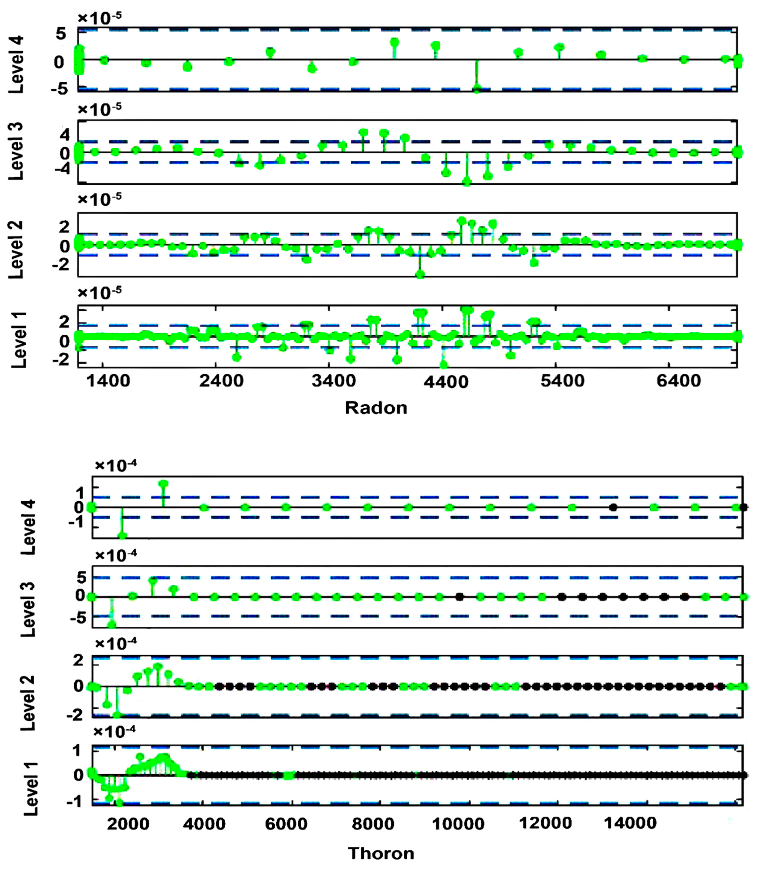
Figure 14.
Wavelet coefficients of air temperature using Bior wavelet.
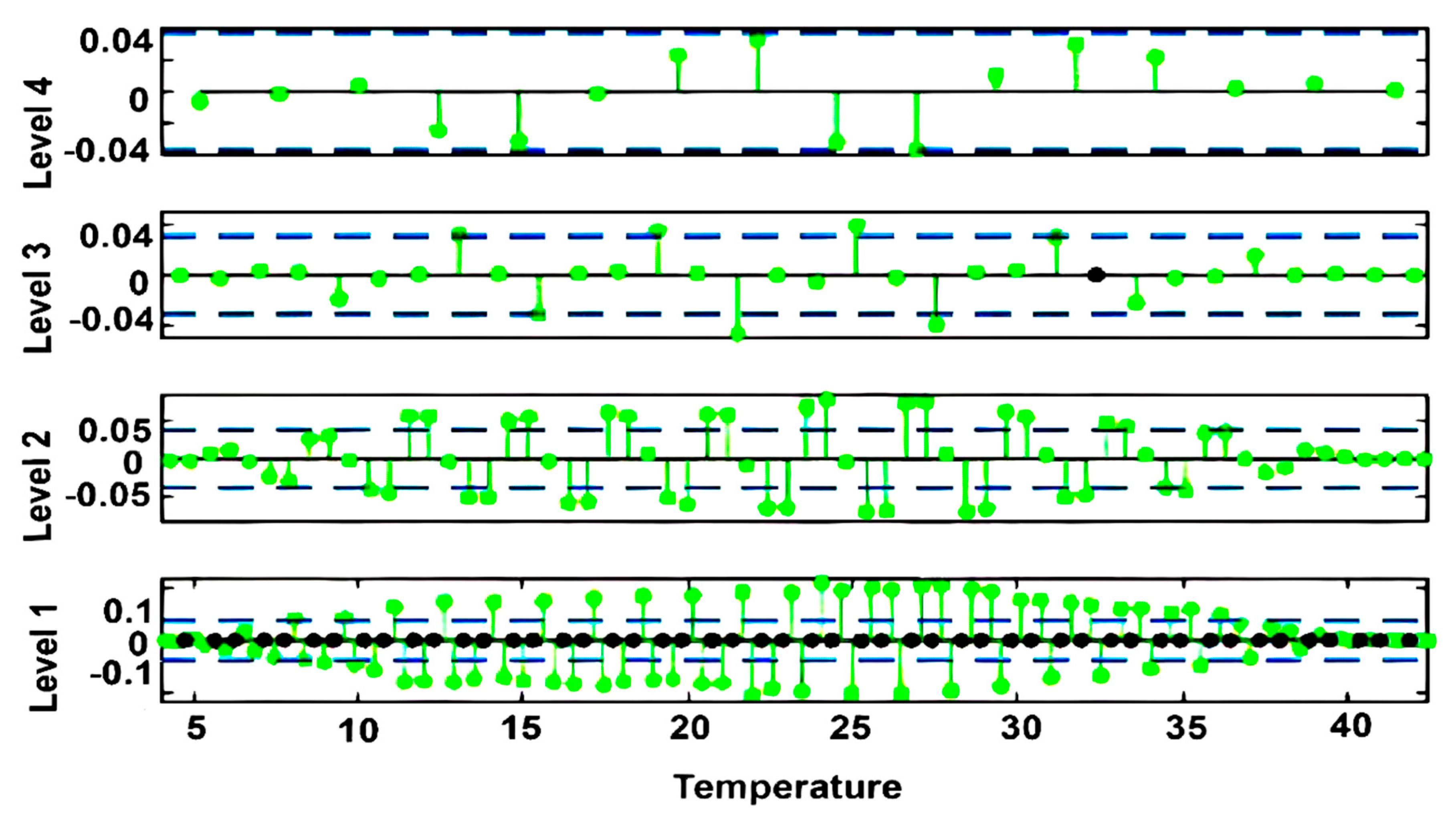
Figure 15.
Wavelet coefficients of air pressure using Bior wavelet.
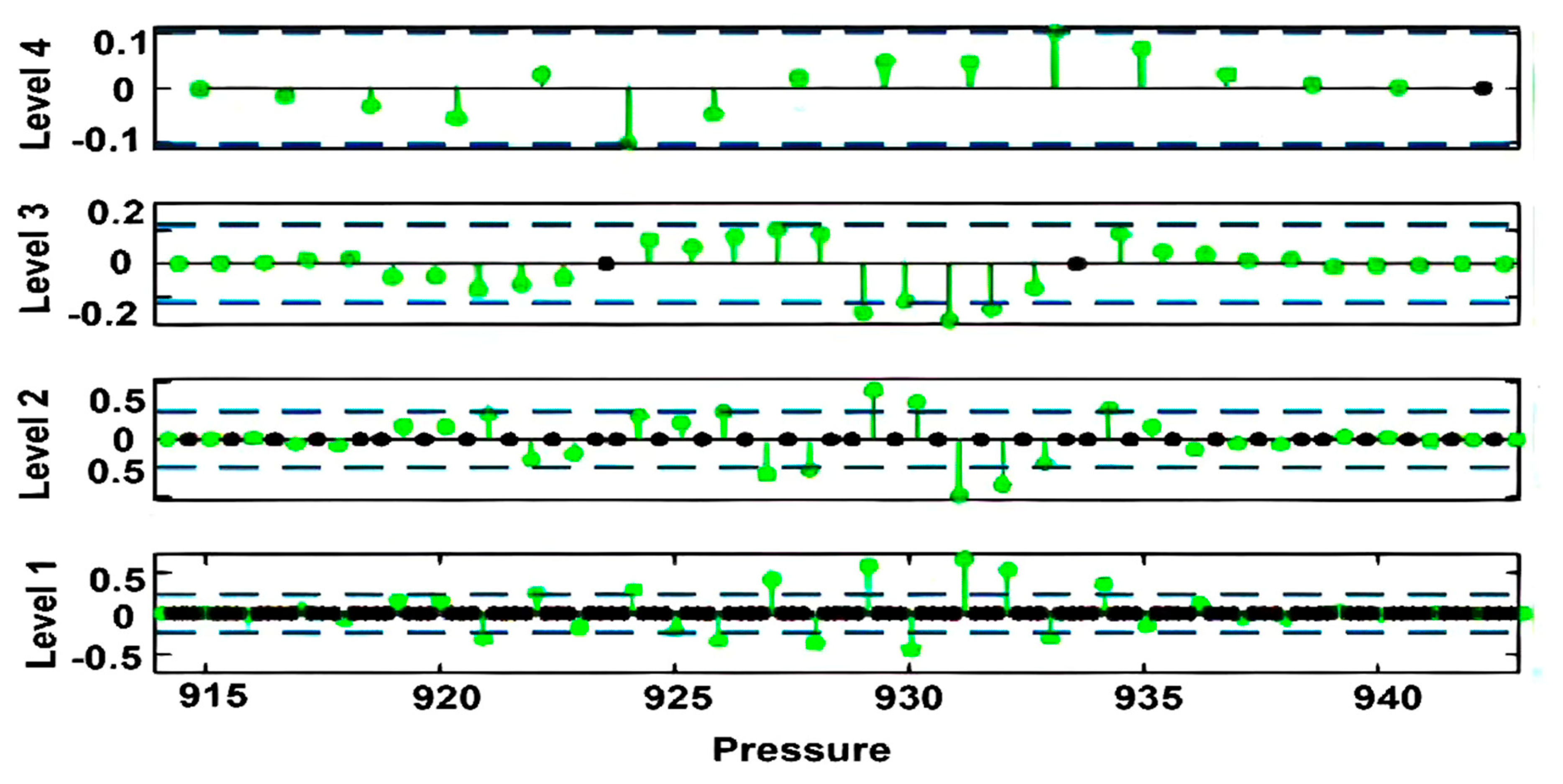
Figure 16.
Wavelet coefficients of air humidity using Bior wavelet.
Up to now, via KDE heat maps, the HBDE method and the four levels of the the wavelet coefficients with the Bior wavelet, it became evident that thoron time series is not affected by the studied meteorological factors. Radon time series are surely not strongly affected and only some bias may be present, mainly, by the atmospheric pressure. To check further if such a bias may affect reason time series Perarson’s correlation matrix was produced. Table 3 presents the main linear correlations between atmospheric-meteorological parameters and radon or thoron time series. As is observed some very low positive correlation of radon is observed with pressure and humidity, (coefficients of 0.121 and 0.432, respectively), whilst radon is negligible negatively correlated with temperature (-0.141). On the other hand, the correlation matrix shows greater effects of the meteorological parameters to thoron time series since the corresponding Parsons’s coefficient are higher. In specific, thoron time series is negligibly positively correlated with temperature, (Pearson’s coefficient of 0.579) and a negligible negative correlation with air pressure and air humidity (Paerson’s coefficients of -0.510 and -0.211, respectively). It can be supported hence, that the potential bias of atmospheric parameters in radon time series (where only the atmospheric pressure shows some increased bias) is not justified by the linear correlation between pressure and radon. Therefore this reinforces the claims that the links between radon time series variations and the earthquakes of Table 1 are the most probable. This is also valid for thoron time series, where the corresponding series is not affected by atmospheric parameter from the other methods, whereas the bias identified from Person’s linear correlation is more prominent (still low though). It can be supported hence from all the evidence presented so far, that the link between the variations of radon and thoron time series and the earthquakes of Table 1 are the most probable.
Figure 17, Figure 18, Figure 19, Figure 20 and Figure 21 present the WBDE plots of radon, thoron, and meteorological time series. As can be observed from Figure 17, low-density areas are observed on 12 March 2017, i.e., 11 days before two earthquakes of magnitudes MW=4.3 (21 March 2017, EQ1) and MW=2.5 (23 March 2017, EQ2). According to Figure 18, anomalous WBDE are observed on 12 March 2017, i.e., 11 days before two earthquakes of magnitudes MW=4.3 (21 March 2017, EQ1) and MW=2.5 (23 March 2017, EQ2). Peaks, valleys and flat areas are observed in the WBDE plots of the meteorological time series, indicating the anomalies in temperature, pressure, and humidity time series data.
4. Conclusions
This study employed the wavelet transform on radon and thoron time seies with Biorthogonal wavelets to separate noise and extract meaningful signals. Kernel density estimation wavelet-based density estimation methods were then applied to detect anomalies in the radon and thoron time series. The outcomes of this study confirm the presence of anomalies in both radon and thoron time series data. Moreover, the links of these anomalies to seismic events that occurred during the study period are also reported. The KDE applied to the radon and thorough time series identified nine significant anomalies. The anomalies in radon time series data were detected on 12 March 2017, 15 August 2017, 17 September 2017 and on 19 January 2018. These anomalies were identified several days before the corresponding seismic events. Anomalies in thoron time series were observed on 12 March 2017, 15 August 2017, 17 September 2017, and on 28 February 2018, all preceding the seismic events by some days. Five out of nine seismic events with anomalies in both radon and thoron time-series data have been accurately were identified by the Kernel Density Estimation technique. WBDE identified four radon anomalies and two thoron anomalies that were associated to the corresponding seismic activities. Future research should focus on refining these techniques and expanding the dataset to enhance the accuracy and reliability of earthquake prediction based on environmental radioactivity measurements. The installation of more radon thoron stations is always a target in the seismic prone areas of Pakistan.
Author Contributions
Conceptualization, M.R. and A.R..; methodology, A.R., M.O.,A.A.M..; software, A.R., Gi.P, C.D., P.Y..; validation, M.R., K.J.K. and S.U.R.; formal analysis, A.R., G.P., D.N., K.K, C.D., Gi.P, P.Y and S.U.R.,; investigation, M.R., A.R., A.A.M., D.N., K.J.K and K.K..; resources, M.R.A.A.M.; data curation, A.R., A.A.M., P.Y..Gi.P., G.P., K.K., C.D and K.J.K; writing—original draft preparation, M.R., A.R. D.N., K.J.K and S.U.R.; writing—review and editing, M.R. and D.N..; visualization, A.R.; supervision, M.R., K.J.K and S.U.R.; project administration, M.R.; funding acquisition, M.R. All authors have read and agreed to the published version of the manuscript.”
Funding
This work was supported by Higher Education Commission (HEC) of Pakistan under Grant No: 6453/AJK/NRPU/R&D/HEC/2016 against the NRPU project executed by one of the authors, M.R.
Institutional Review Board Statement
Not applicable.
Informed Consent Statement
Not applicable.
Data Availability Statement
Data is unavailable due to ethical restrictions.
Acknowledgments
We are thankful to Dr. Aleem Dad Khan Tareen for his efforts in data collection. Special thanks are due to Dr. Tayyib Riaz from the Institute of Geology, University of Azad Jammu and Kashmir, for his invaluable assistance in drafting the geological map and contributing to the geological aspects of the manuscript. Additionally, one of the authors, M.R., sincerely acknowledges the Higher Education Commission of Pakistan for providing funding that facilitated the completion of the project, of which this study is a part.
Conflicts of Interest
Authors declare that “The funders had no role in the design of the study; in the collection, analyses, or interpretation of data; in the writing of the manuscript; or in the decision to publish the results”.
References
- Woith, H.; Petersen, G.; Hainzl, S.; Dahm, T. Review: Can Animals Predict Earthquakes? Bull. Seismol. Soc. Am. 2018, 108, 1031–1045. [Google Scholar] [CrossRef]
- Wuyep, L.C; Kadiri, U.A.; Monday, I.A.; Nansak, N.E. Z, L.T.,; Habila Y.O.; Ezisi P. Geo-Chemical Techniques for Earthquake Forecasting in Nigeria. Asian J. Geogr. Res.. 2021, 4, 29–45, AJGR.72897. [Google Scholar] [CrossRef]
- Placinta, A.O.; Borleanu, F.; Moldovan, I.A.; Coman, A. Correlation between Seismic Waves Velocity Changes and the Occurrence of Moderate Earthquakes at the Bending of the Eastern Carpathians (Vrancea). Acoust. 2022, 4, 934–947. [Google Scholar] [CrossRef]
- Cao, B.; Ge, Z. Cascading multi-segment rupture process of the 2023 Turkish earthquake doublet on a complex fault system revealed by teleseismic P wave back projection method. Earthq. Sci. 2024, 37, 158–173. [Google Scholar] [CrossRef]
- Nikolopoulos, D.; Cantzos, D.; Alam, A.; Dimopoulos, S.; Petraki, E. Electromagnetic and Radon Earthquake Precursors. Geosciences 2024, 14, 271. [Google Scholar] [CrossRef]
- Conti, L.; Picozza, P.; Sotgiu, A. A Critical Review of Ground Based Observations of Earthquake Precursors. Front. Earth Sci. 2021, 9, 676766. [Google Scholar] [CrossRef]
- Tsuchiya, M.; Nagahama, H.; Muto, J.; Hirano, M.; Yasuoka, Y. Detection of atmospheric radon concentration anomalies and their potential for earthquake prediction using Random Forest analysis. Sci. Rep. 2024, 14, 11626. [Google Scholar] [CrossRef]
- Chetia, T.; Baruah, S.; Dey, C.; Baruah, S.; Sharma, S. Seismic induced soil gas radon anomalies observed at multiparametric geophysical observatory, Tezpur (Eastern Himalaya), India: An appraisal of probable model for earthquake forecasting based on peak of radon anomalies. Nat. Hazards 2022, 111, 3071–3098. [Google Scholar] [CrossRef]
- Romano, D.; Sabatino, G.; Magazù, S.; Bella, M.D.; Tripodo, A.; Gattuso, A.; Italiano, F. Distribution of soil gas radon concentration in north-eastern Sicily (Italy): Hazard evaluation and tectonic implications. Environ. Earth Sci. 2023, 82, 273. [Google Scholar] [CrossRef]
- Pulinets, S.; Herrera, V.M.V. Earthquake Precursors: The Physics, Identification, and Application. Geosciences 2024, 14, 209. [Google Scholar] [CrossRef]
- World Health Organisation (WHO) Radon. 2025. Available online: https://www.who.int/news-room/fact-sheets/detail/radon-and-health (accessed on 23 October 2025).
- Kashkinbayev, Y.; Bakhtin, M.; Kazymbet, P.; Lesbek, A.; Kazhiyakhmetova, B.; Hoshi, M.; Altaeva, N.; Omori, Y.; Tokonami, S.; Sato, H.; et al. Influence of Meteorological Parameters on Indoor Radon Concentration Levels in the Aksu School. Atmosphere 2024, 15, 1067. [Google Scholar] [CrossRef]
- Huang, P.; Lv, W.; Huang, R.; Feng, Y.; Luo, O.; Yin, C.; Yang, Y. Impact of environmental factors on atmospheric radon variations at China Jinping Underground Laboratory. Sci. Rep. 2024, 14, 31402. [Google Scholar] [CrossRef]
- Huang, C. Featured anomaly detection methods and applications. PhD thesis, University of Exeter, Computer Science Department, United Kingdom, June 2018. [Google Scholar]
- Rafique, M.; Tareen, A.D.K.; Mir, A.A.; Sajjad, M.; Nadeem, A.; Asim, K.M.; Kearfott, K.J. Delegated Regressor, A Robust Approach for Automated Anomaly Detection in the Soil Radon Time Series Data. Sci. Rep. 2020, 10, 3004. [Google Scholar] [CrossRef]
- Chen, Y.C. A Tutorial on Kernel Density Estimation and Recent Advances. Biostatistics & Epidemiology 2017, 1. [Google Scholar] [CrossRef]
- Parzen, E. On Estimation of a Probability Density Function and the Mode. The Annals of Mathematical Statistics 1962, 33, 1065–1076. [Google Scholar] [CrossRef]
- Laxhammar, R.; Falkman, G.; Sviestins, E. Anomaly detection in sea traffic - A comparison of the Gaussian Mixture Model and the Kernel Density Estimator. In Proceedings of the 2th International Conference on Information Fusion, Seattle, WA, USA, 6–9 July 2009; pp. 756–763. https://ieeexplore.ieee.org/document/5203766.
- Ramanna, C. K.; Dodagoudar, G. R. Seismic hazard analysis using the adaptive Kernel density estimation technique for Chennai City. Pure Appl. Geophys. 2012, 169, 55–69. [Google Scholar] [CrossRef]
- Zhang, L.; Lin, J.; Karim, R. Adaptive kernel density-based anomaly detection for nonlinear systems. Knowledge-Based Systems 2018, 139, 50–63. [Google Scholar] [CrossRef]
- Kordestani, M.; Alkhateeb, A.; Rezaeian, I.; Rueda, L.; Saif, M. A new clustering method using wavelet based probability density functions for identifying patterns in time-series data. In Proceedings of the 2016 IEEE EMBS International Student Conference (ISC), Ottawa, ON, Canada; 2016; pp. 1–4. [Google Scholar] [CrossRef]
- García-Treviño, E.S.; Barria, J.A. Online wavelet-based density estimation for non-stationary streaming data, Comput. Stat. Data Anal. 2012, 56, 327–344. [Google Scholar] [CrossRef]
- Ayub, M.; Rahman, A.-U.; Samiullah; Khan, A. Extent and evaluation of flood resilience in Muzaffarabad City, Azad Jammu and Kashmir, Pakistan. Journal of Himalayan Earth Sciences 2021, 54, 14–27. [Google Scholar]
- Baig, M. S.; Lawrence, R.D.; Snee, L.W. Precambrian to early Cambrian orogeny in the northwest Himalaya, Pakistan. Geolog. Mag. 1988, 125, 83–86. [Google Scholar] [CrossRef]
- Alam, A.; Wang, N.; Zhao, G.; Barkat, A. Implication of Radon Monitoring for Earthquake Surveillance Using Statistical Techniques: A Case Study of Wenchuan Earthquake Geofluids. 2020, 2429165. [Google Scholar] [CrossRef]
- Kaneda, H.; Nakata, T.; Tsutsumi, H.; Kondo, H.; Sugito, N.; Awata, Y.; Kausar, A.B. Surface rupture of the 2005 Kashmir, Pakistan, earthquake and its active tectonic implications. Bull. Seismol. Soc. Am. 2008, 98, 521–557. [Google Scholar] [CrossRef]
- USGS (United States Geological Survey), M 7.6 - 21 km NNE of Muzaffarabad, Pakistan- Pakistan earthquake 2005. Available online: https://earthquake.usgs.gov/earthquakes/eventpage/usp000e12e/executive (accessed on 30 October 2025).
- SARAD GmbH. 2025. Available online: https://www.sarad.de/product-detail.php (accessed on 30 October 2025).
- National Seismic Monitoring Centre, Islamabad. Available online: https://seismic.pmd.gov.pk/(accessed on Saturday, 1 November, 2025 10:01 PM).
- Dobrovolsky, I.P.; Zubkov, S.I.; Miachkin, V.I. Estimation of the size of earthquake preparation zones. Pure Appl. Geophys. 1979, 117, 1025–1044. [Google Scholar] [CrossRef]
- Danese, M.; Lazzari, M.; Murgante, B. Kernel Density Estimation Methods for a Geostatistical Approach in Seismic Risk Analysis: The Case Study of Potenza Hilltop Town (Southern Italy). In Lecture Notes in Computer Science Computational Science and Its ApplicationICCSA 2008; Gervasi, O., Murgante, B., Laganà, A., Taniar, D., Mun, Y., Gavrilova, M.L., Eds.; Springer: Berlin, Heidelberg, 2008; Volume 5072, pp. 415–429. [Google Scholar] [CrossRef]
- Amador Luna, D.; Alonso-Chaves, F.M.; Fernández, C. Kernel Density Estimation for the Interpretation of Seismic Big Data in Tectonics Using QGIS: The Türkiye–Syria Earthquakes (2023). Remote Sens. 2024, 16, 3849. [Google Scholar] [CrossRef]
- Murphy, K.P. Machine learning - a probabilistic perspective. In Adaptive computation and machine learning series. 2012. Available online: https://api.semanticscholar.org/CorpusID:17793133.
- Frehner, R.; Wu, K.; Sim, A.; Kim, J.; Stockinger, J. Detecting Anomalies in Time Series Using Kernel Density Approaches. IEEE Access 2024, 12, 33420–33439. [Google Scholar] [CrossRef]
- Hu, W.; Gao, J.; Li, B.; Wu, O.; Du, J.; Maybank, S. Anomaly Detection Using Local Kernel Density Estimation and Context-Based Regression. IEEE Trans. Knowl. Data Eng. 2020, 32, 218–233. [Google Scholar] [CrossRef]
- Torshizian, H.; Afzal, P.; Rahbar, K.; Yasrebi, A.B.; Wetherelt, A.; Fyzollahhi, N. Application of modified wavelet and fractal modeling for detection of geochemical anomaly. Geochem 2021, 81, 125800. [Google Scholar] [CrossRef]
- Yao, Y.; Ma, J.; Ye, Y. Regularizing autoencoders with wavelet transform for sequence anomaly detection. Pattern Recognit. 2023, 134, 109084. [Google Scholar] [CrossRef]
- Jiang, Z.; Rashid, M.M; Johnson, F.; Sharma, A. A wavelet-based tool to modulate variance in predictors: An application to predicting drought anomalies. Environmental Modelling & Software 2021, 135, 104907. [Google Scholar] [CrossRef]
- Miao, C.; Dong, Q.; Hao, M.; Wang, C.; Cao, J. Magnetic anomaly detection based on fast convergence wavelet artificial neural network in the aeromagnetic field. Measurement 2021, 176, 109097. [Google Scholar] [CrossRef]
- Halidou, A.; Mohamadou, Y.; Ari, A. A. A.; Zacko, E. J. G. Review of wavelet denoising algorithms. Multimed. Tools Appl. 2023, 82, 41539–41569. [Google Scholar] [CrossRef]
- Rasheed, A.; Osama, M.; Rafique, M.; Tareen, A.D.K.; Lone, K.J.; Qureshi, S.A.; Kearfott, K.J.; Aftab, A.; Nikolopoulos, D. Time-frequency analysis of radon and thoron data using continuous wavelet transform. Phys. Scr. 2023, 98, 105008. [Google Scholar] [CrossRef]
- Arfaoui, S.; Ben Mabrouk, A.; Cattani, C. Wavelet Analysis: Basic Concepts and Applications, 1st ed.; Chapman and Hall/CRC: New York, NY, US, 2021; pp. 1–254, eBook ISBN 9781003096924. [Google Scholar] [CrossRef]
- Caudle, K. A.; Wegman, E. Nonparametric density estimation of streaming data using orthogonal series. Comput. Stat. Data Anal. 2009, 53, 3980–3986. [Google Scholar] [CrossRef]
- Jiang, Z.; Sharma, A.; Johnson, F. mAssessing the sensitivity of hydro-climatological change detection methods to model uncertainty and bias. Advances in Water Resources 2019, 134, 103430. [Google Scholar] [CrossRef]
- Scott, N.V.; Barnard, V.O. Optimal Location Estimation and Anomaly Quantification for a Mobile Information Carrier: Prior Feeds for Deep Learning. In Proceedings of the 8th International Conference on Civil, Structural and Transportation Engineering, Carleton University, Ottawa, Canada, 4–6 June 2023; Avestia Publishing article number 111. [Google Scholar] [CrossRef]
- Beyene, T.K.; Jain, M.K.; Yadav, B.K.; Agarwal, A. Multiscale investigation of precipitation extremes over Ethiopia and teleconnections to large-scale climate anomalies. Stoc. Env. Res. Risk 2022, 36, 1503–1519. [Google Scholar] [CrossRef]
Figure 1.
Regional tectonic map of the westernmost part of the frontal Himalaya. (Adopted from Kaneda et al. [26]).
Figure 1.
Regional tectonic map of the westernmost part of the frontal Himalaya. (Adopted from Kaneda et al. [26]).
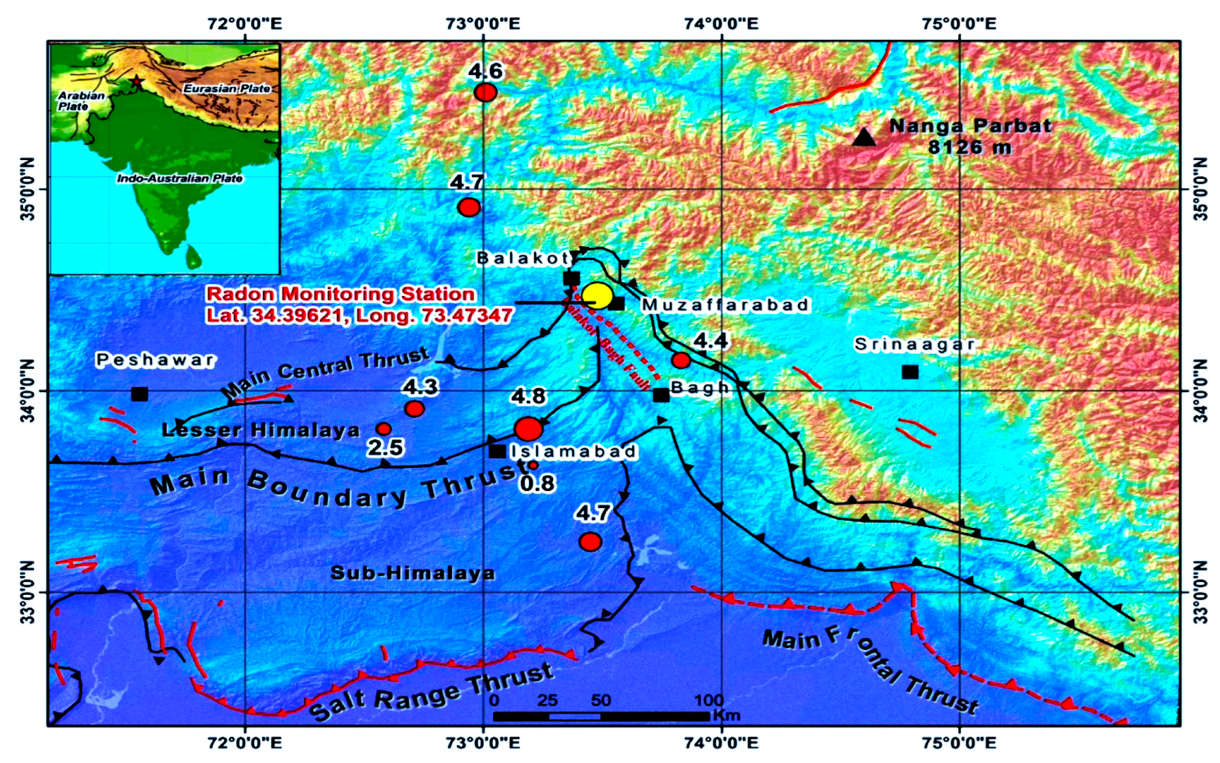
Figure 2.
KDE estimation of radon time series.
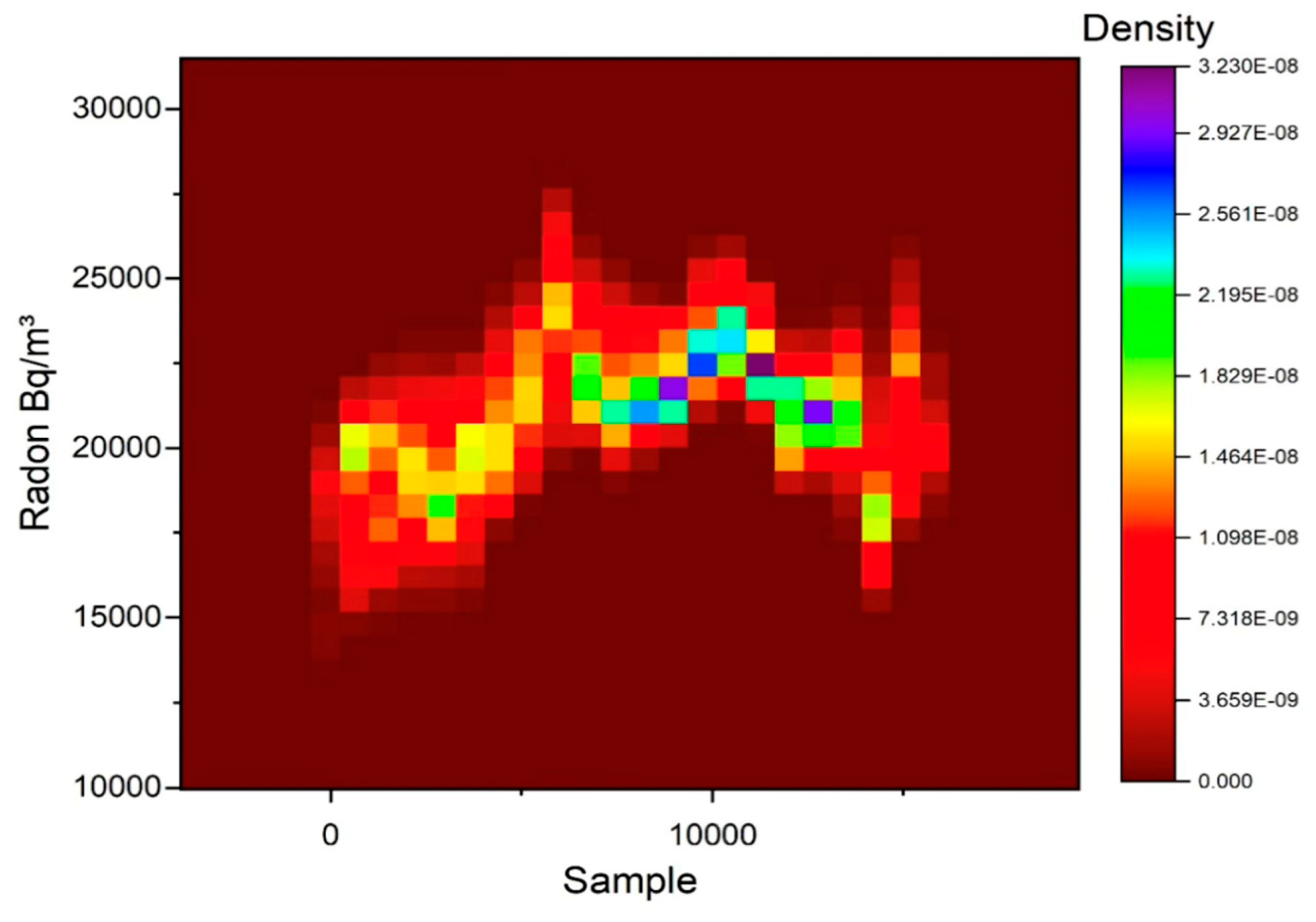
Figure 3.
KDE estimation of radon time series.
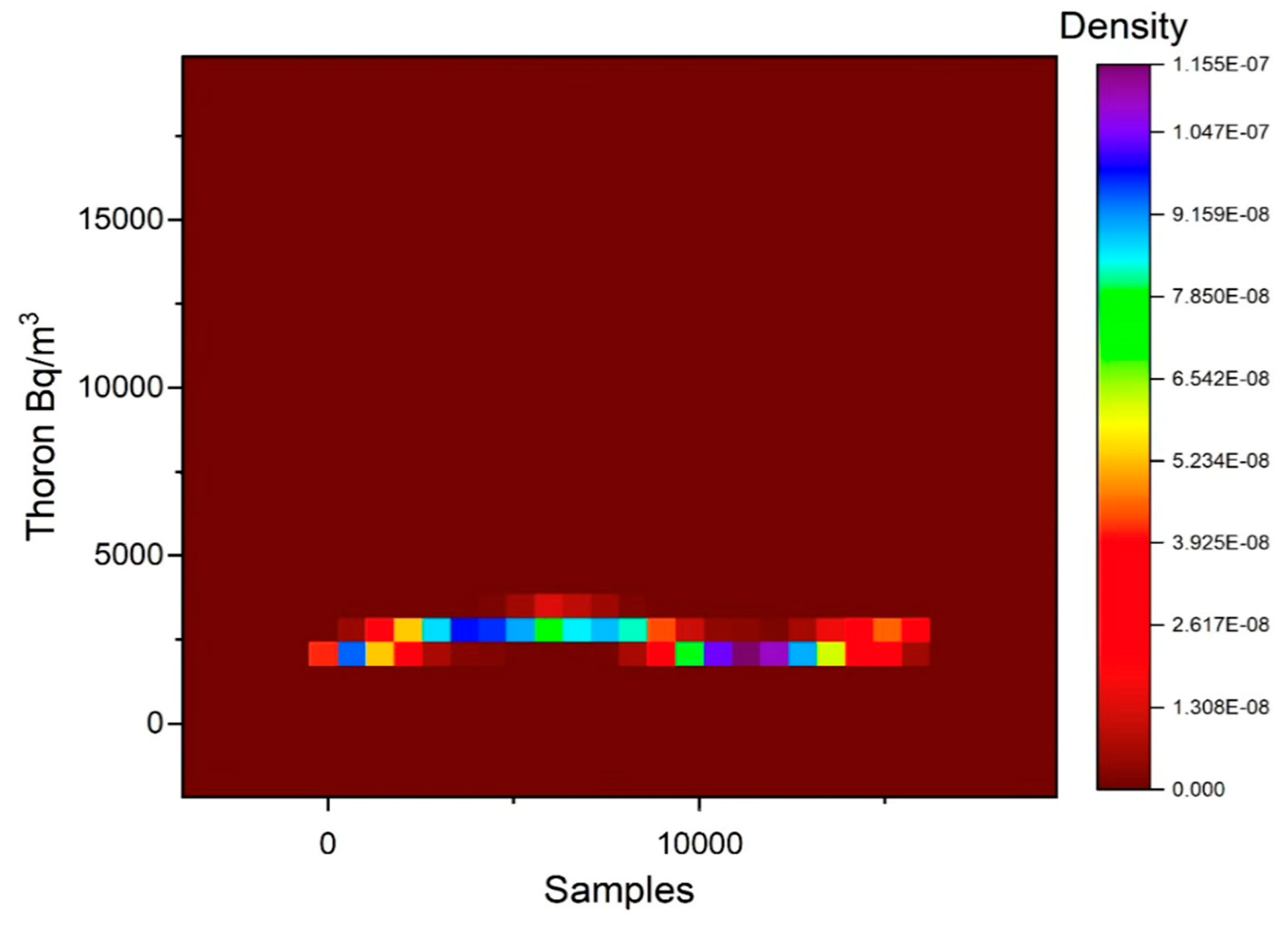
Figure 4.
KDE estimation of temperature time series (Temp).
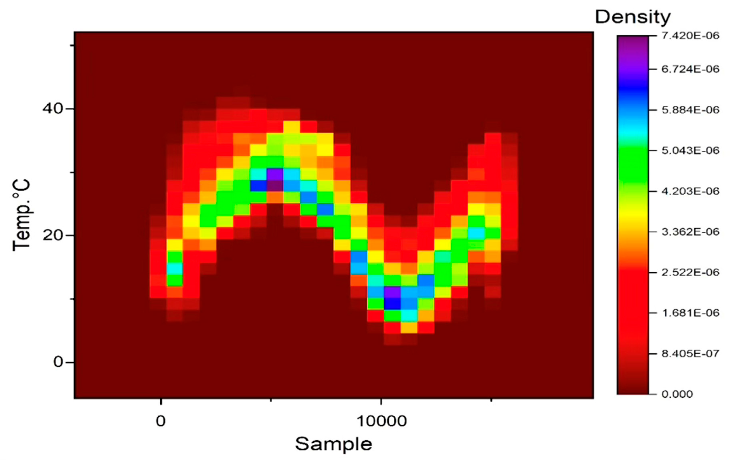
Figure 5.
KDE estimation of atmospheric pressure time series.
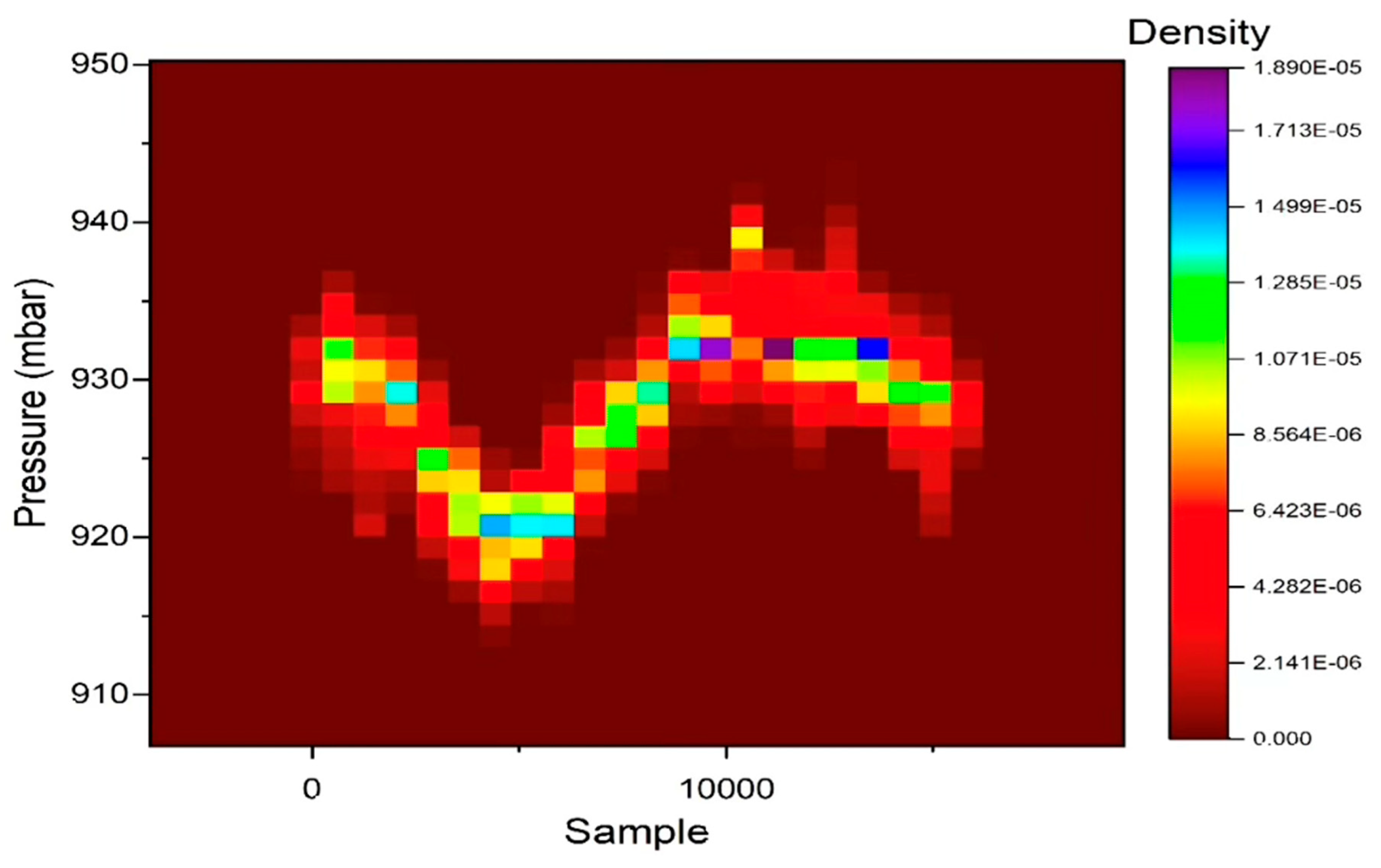
Figure 6.
KDE estimation of atmospheric humidity time series.
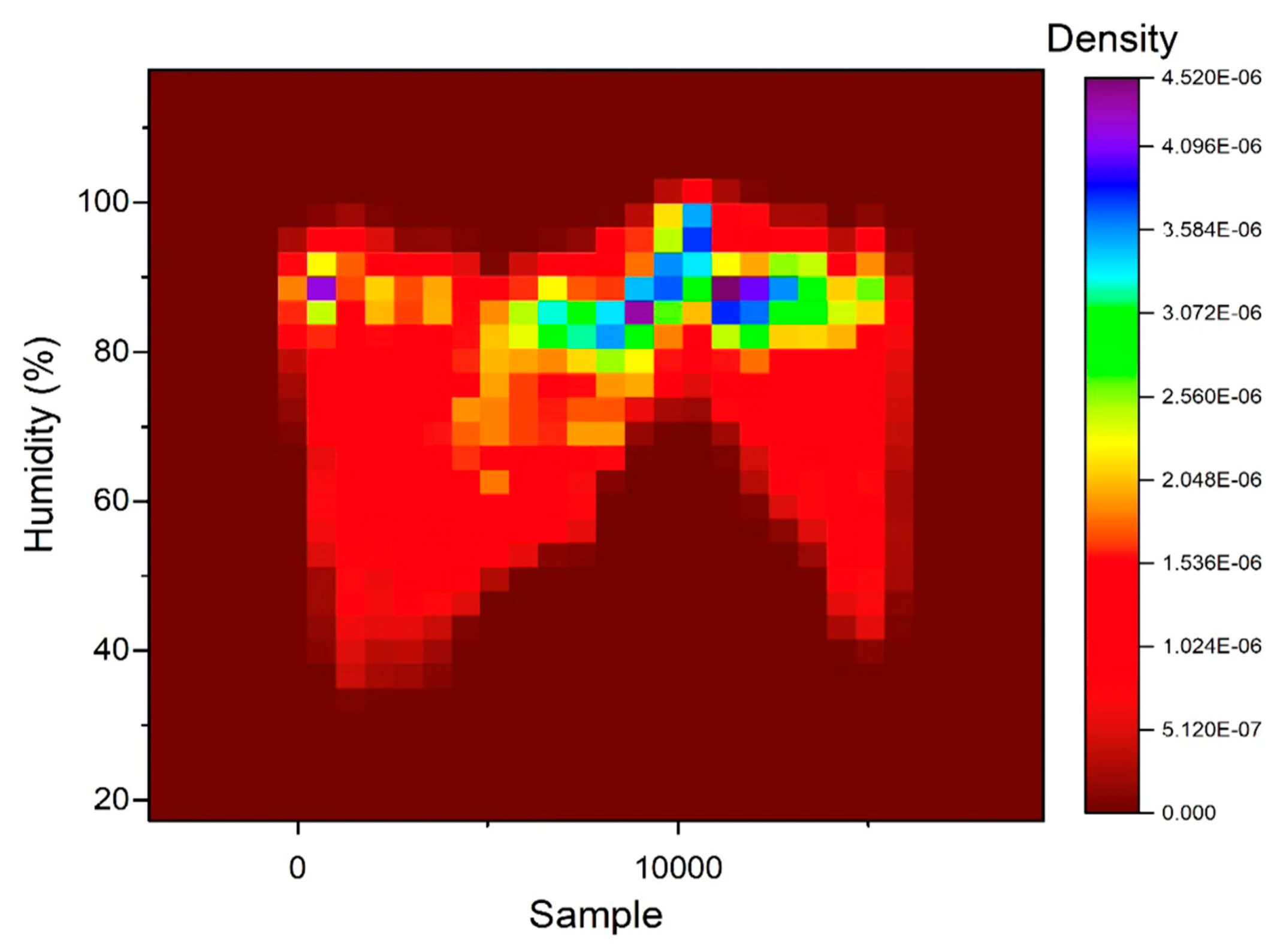
Figure 7.
HBDE estimation of thoron time series.
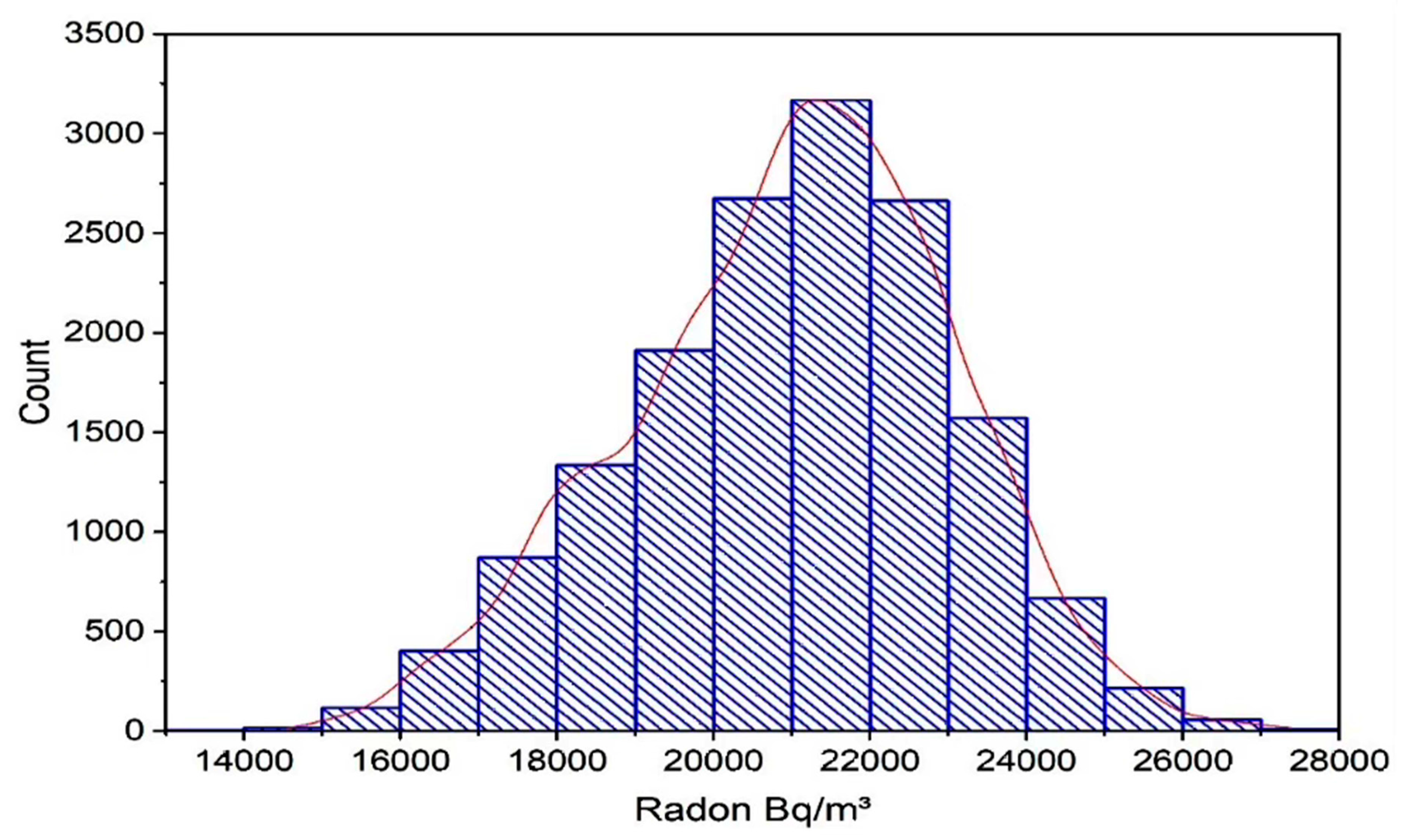
Figure 8.
HBDE estimation of thoron time serie.
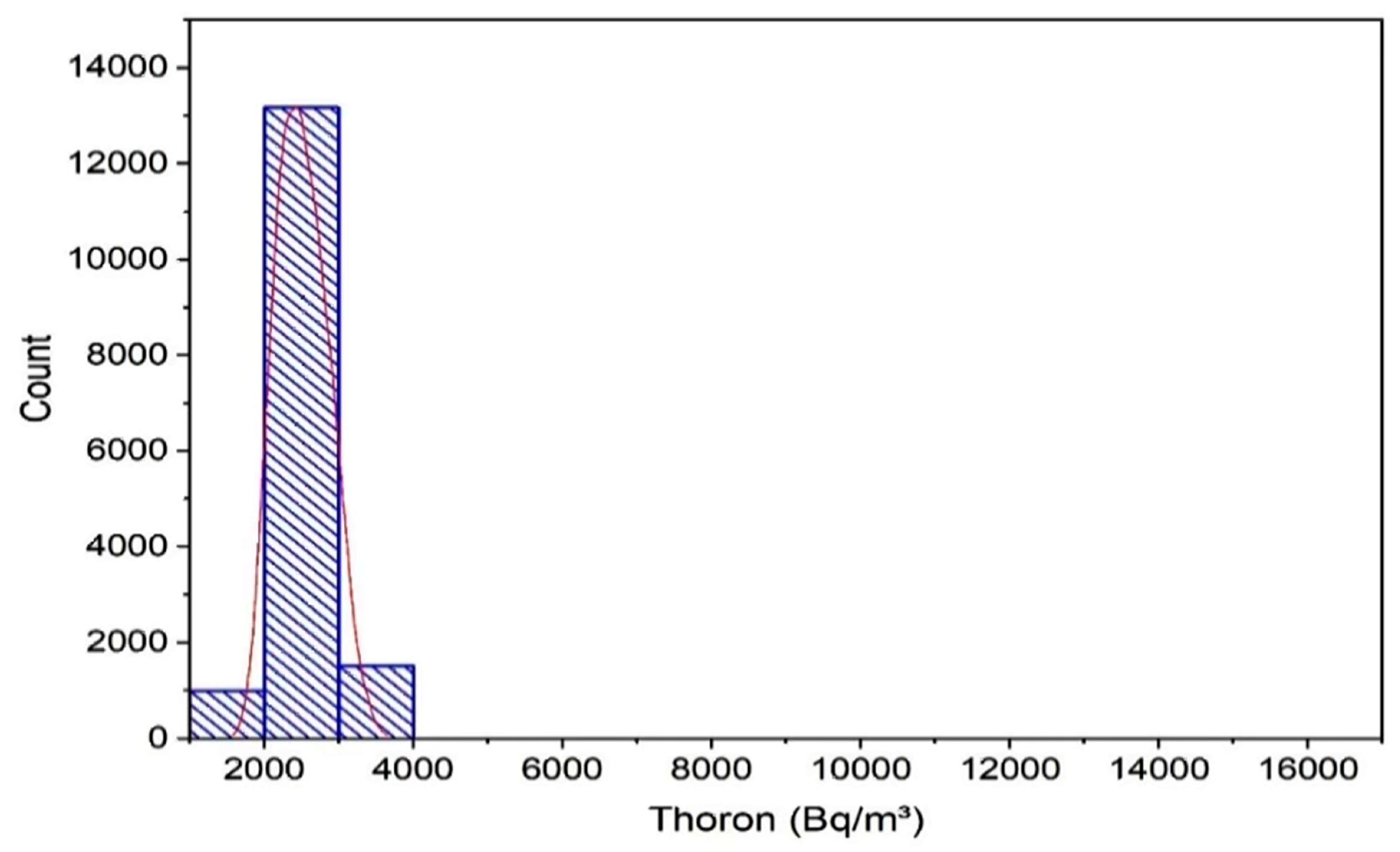
Figure 9.
HBDE estimation of temperature time series (Temp).
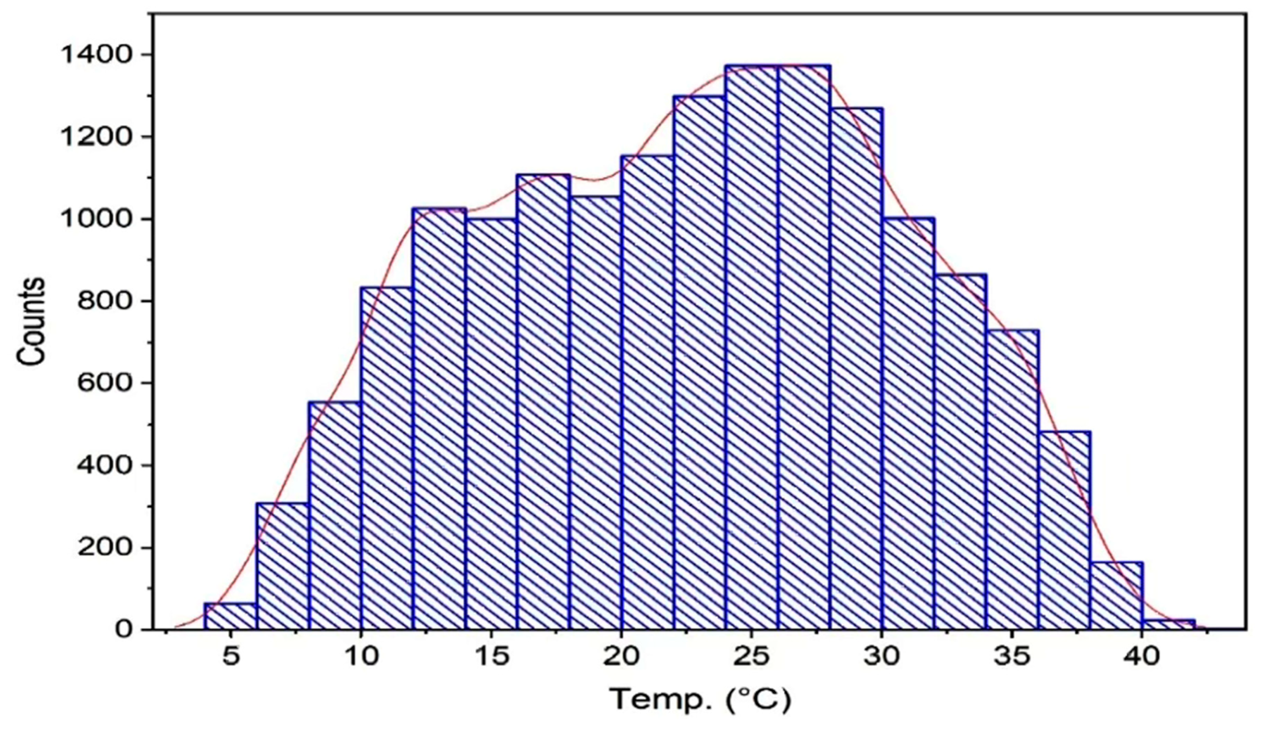
Figure 10.
HBDE estimation of air pressure time series.
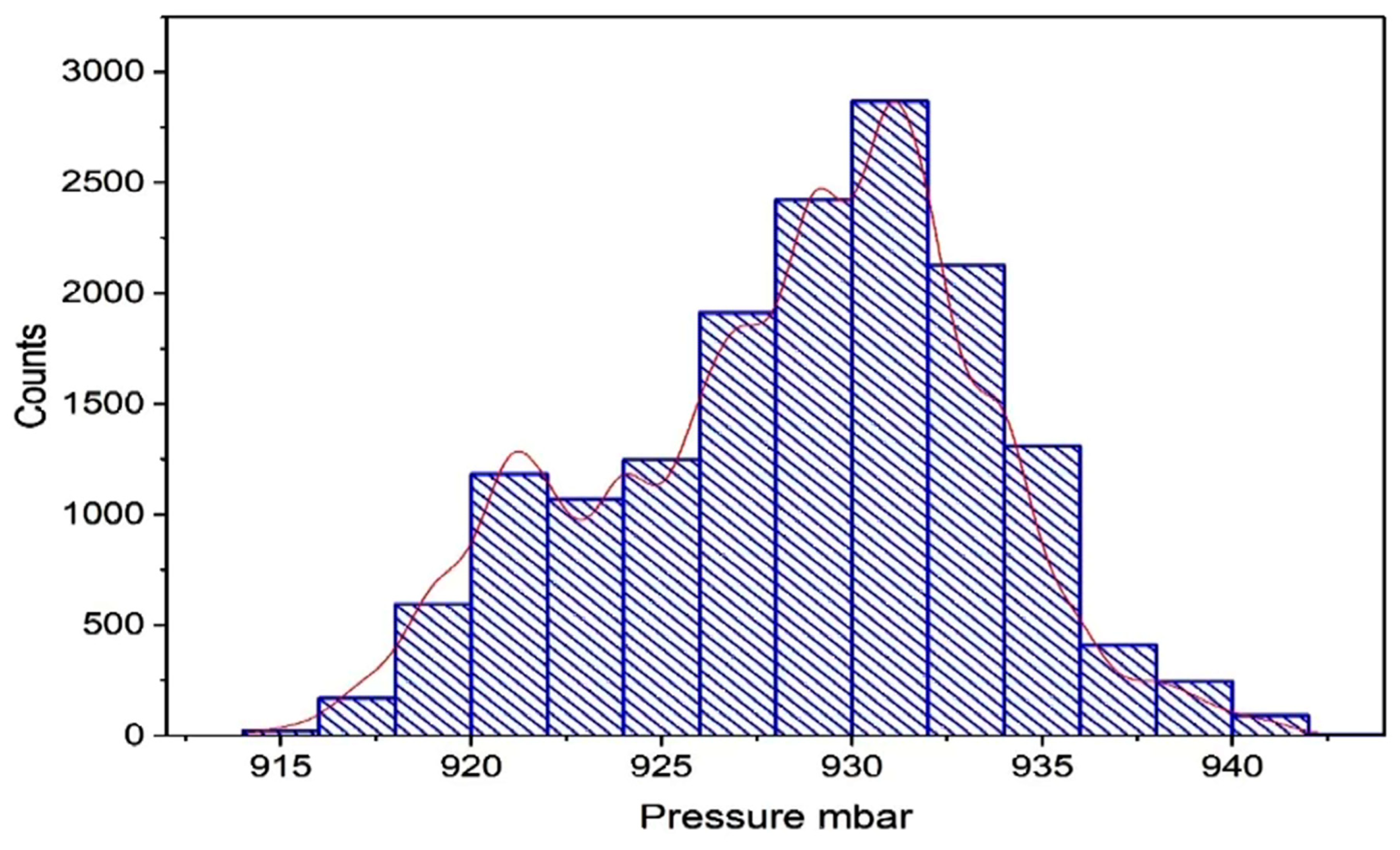
Figure 11.
HBDE estimation of air humidity time series.
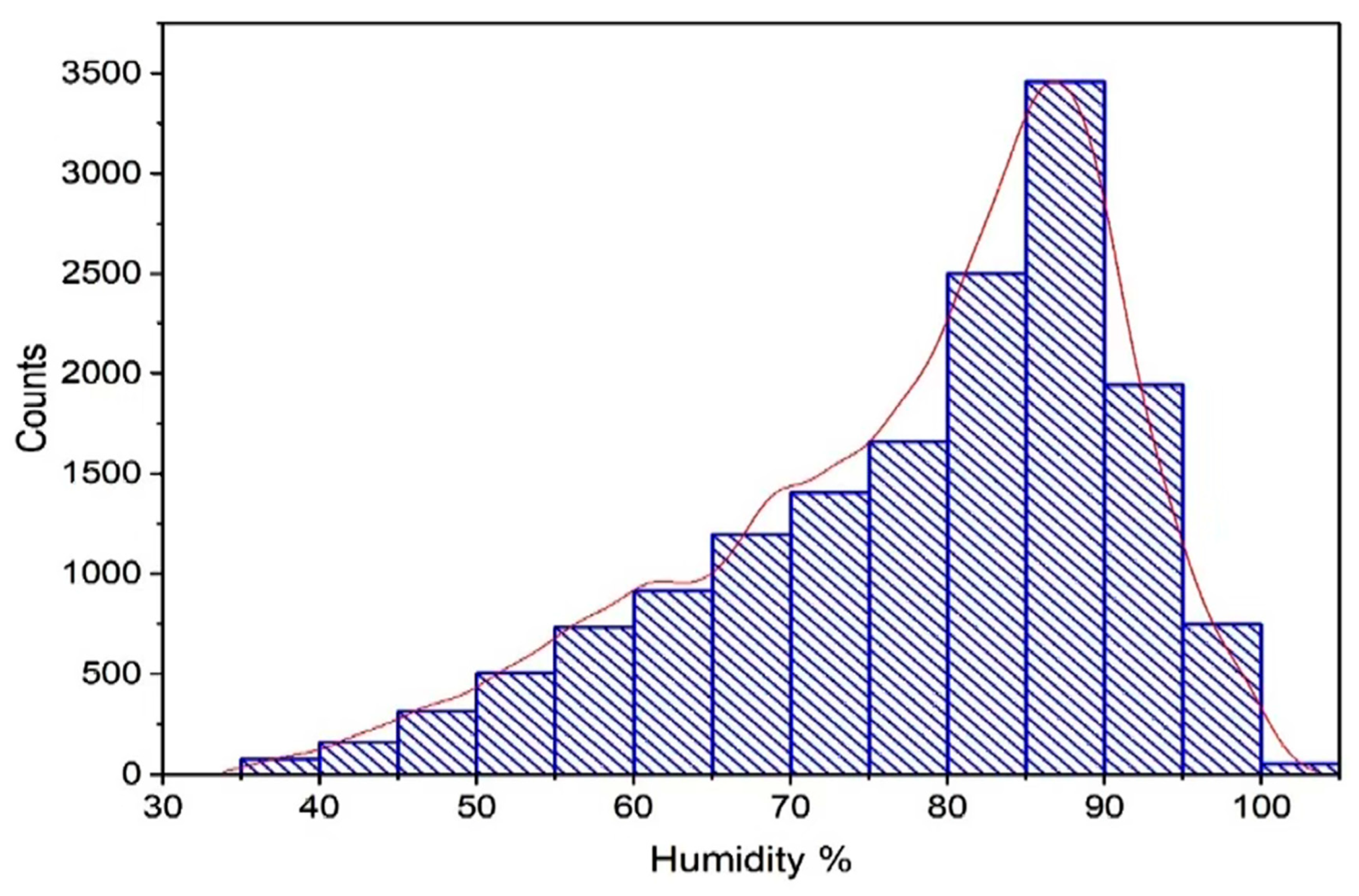
Figure 17.
Wavelet-based density of radon.
Figure 18.
Wavelet-based density of thoron.
Figure 19.
Wavelet-based density of temperature.
Figure 20.
Wavelet-based density of air pressure.
Figure 21.
Wavelet-based density of air humidity.

Table 1.
Data for the selected earthquakes. EQ represent the number of the earthquake. is the epicentral distance from the radon-thorn station and is the earthquake preparation radius (both in 4 significant figures). The columns 2-7 have been downloaded by the National Seismic Monitoring Centre of Pakistan [29].
| EQ | Date | Magnitude | Latitude N |
Longitude E |
Depth (km) |
(km) |
(km) |
|---|---|---|---|---|---|---|---|
| EQ1 | 21/03/2017 | 4.3 | 33.91 N | 72.71 E | 25 | 86.00 | 70.60 |
| EQ2 | 23/03/2017 | 2.5 | 33.81 N | 72.58 E | 156 | 103.0 | 11.89 |
| EQ3 | 27/08/2017 | 4.8 | 33.81 N | 73.19 E | 10 | 66.34 | 115.9 |
| EQ4 | 23/09/2017 | 4.6 | 35.48 N | 73.01 E | 61 | 135.0 | 95.06 |
| EQ5 | 09/12/2017 | 4.7 | 33.25 N | 76.45 E | 101 | 300.0 | 104.9 |
| EQ6 | 03/02/2018 | 0.8 | 33.63 N | 73.21 E | 157 | 142.9 | 2.208 |
| EQ7 | 28/02/2018 | 4.4 | 34.15 N | 73.83 E | 134 | 41.78 | 77.98 |
| EQ8 | 14/03/2018 | 4.9 | 33.93 N | 77.12 E | 10 | 343.0 | 127.9 |
| EQ9 | 15/03/2018 | 4.7 | 33.1 N | 76.14 E | 45 | 284.5 | 105.0 |
Table 2.
Kernel density estimation and wavelet based density estimation in three significant figures for the earthquakes of Table 1. EQ represent the number of the earthquake of Table 1. Cut-off limits for the density values are also presented.
| EQ | Radon time series | Thoron time series | |||
|---|---|---|---|---|---|
| KDE | WBDE | KDE | WBDE | ||
| EQ1 | 1.46E-08 | 0.11E-04 | 1.30E-08 | 4.63E-04 | |
| EQ2 | 1.09E-08 | 0.26E-04 | 2.62E-08 | 6.71E-04 | |
| EQ3 | 1.83E-08 | 0.95E-04 | 7.85E-08 | 0.12E-04 | |
| EQ4 | 1.46E-08 | 1.23E-04 | 9.16E-08 | 0.12E-04 | |
| EQ5 | 2.19E-08 | 1.12E-04 | 9.16E-08 | 0.12E-04 | |
| EQ6 | 7.32E-09 | 1.56E-04 | 1.55E-07 | 0.12E+04 | |
| EQ7 | 2.93E-08 | 0.42E+04 | 1.05E-07 | 0.12E+04 | |
| EQ8 | 3.65E-09 | 0.31E+04 | 3.93E-08 | 0.12E+04 | |
| EQ9 | 7.32E -09 | 0.11E+04 | 2,62E-08 | 0.12E+04 | |
| Cut-off limit | 3.14E -08 | 4.14E+03 | 1.63E -07 | 1,80E +02 | |
Table 3.
Pearson’s Correlation Coefficient between radon, and thoron with meteorological parameters.
Table 3.
Pearson’s Correlation Coefficient between radon, and thoron with meteorological parameters.
| Type of Variables | Pearson Correlation Coefficient |
|---|---|
| Radon vs Temperature | -0.141 |
| Radon vs Pressure | 0.121 |
| Radon vs Humidity | 0.432 |
| Thoron vs Temperature | 0.579 |
| Thoron vs Pressure | -0.510 |
| Thoron vs Humidity | -0.211 |
Disclaimer/Publisher’s Note: The statements, opinions and data contained in all publications are solely those of the individual author(s) and contributor(s) and not of MDPI and/or the editor(s). MDPI and/or the editor(s) disclaim responsibility for any injury to people or property resulting from any ideas, methods, instructions or products referred to in the content. |
© 2025 by the authors. Licensee MDPI, Basel, Switzerland. This article is an open access article distributed under the terms and conditions of the Creative Commons Attribution (CC BY) license (http://creativecommons.org/licenses/by/4.0/).
Copyright: This open access article is published under a Creative Commons CC BY 4.0 license, which permit the free download, distribution, and reuse, provided that the author and preprint are cited in any reuse.


