
Submitted:
06 November 2025
Posted:
11 November 2025
You are already at the latest version
Abstract
This paper analyses a power system based on the IEEE-57 bus case, integrating thermal and wind generation to meet hourly demand. Using day-ahead wind forecasts as firm market offers, the optimal Pareto front for thermal dispatch is computed, balancing total cost and emissions. The system operator selects a dispatch point based on the desired cost-emissions trade-off.
To reflect real-world uncertainty, the study incorporates statistical deviations in actual wind output derived from historical data. For each deviation scenario, new optimal thermal dispatch curves are generated. This approach enables pre-emptive scheduling across the full range of expected wind deviations and supports real-time adjustment via mechanisms such as redispatch, intraday markets, or secondary/tertiary regulation.
Keywords:
wind power
; forecast error
; Pareto front
; optimal power flow
1. Introduction
Electrical systems used to be based primarily on the use of fossil fuels, with the support of the hydraulic energy and nuclear power, which could be more or less representative depending on the country. But climate change and other atmospheric effects, that have brought a reasonable increase in environmental awareness, and the development of renewable generation technologies, have changed the scene, and nowadays one can see a significant presence, above all, of wind and solar energy, and a tightening of the environmental requirements for thermal power plants to participate in production.
Traditionally, the objective consisted of covering the demand at the lowest possible cost for the system or, in the case of having an electricity market, the economic benefit was sought. Little by little, environmental conditions have been gaining weight when determining the optimal generation mix. or particulate emissions are conditioning conventional thermal generation. However, the decision to emit less leads to higher generation costs, as cleaner fuels and cleaner thermal technologies are more expensive. It seems that the cost and emission objectives are in conflict, they go in opposite directions, and that fact forces us to analyze which could be the best solution, according to each case. A good tool for that study is the use of techniques of multiobjective optimization, and the determination of the Pareto fronts that find the optimal production points for the whole range of possible emissions, making it feasible to analyze all the possibilities, and offering a tool for the generation manager to decide which generation mix to use.
Renewable energies are gaining more and more weight in electrical systems. For example, in the case of Spain, wind and solar energy covered 23.2% and 17% of the demand respectively in plant terminals in 2024. If all renewable energies are added, they accounted for 56.8% of the demand. This indicates that these types of technologies have a very important weight in many electrical systems, and they will grow continuously in the future; therefore, it seems quite interesting to study how renewable energies can influence multi-objective optimization and the relationships between costs and emissions.
Although it seems certain that it will change, there are many countries around the world in which thermal generation continues to play a crucial role in meeting demand, and globally, in the world, coal and gas continue to be the two main sources of electricity production, representing 34% and 22% of the total respectively in 2024. Countries such as Australia, South Africa, China, India, Indonesia or Poland have coal as the main source of electricity production, and at the same time all the countries are in turn promoting the implementation of renewable generation and the limitation of greenhouse gas emissions. Although coal is the least clean thermal source, reasons such as economics, lack of international political stability, security of supply, and the desire to have dispatchable power plants on the electricity grid may make it difficult to replace it with gas-fired plants and renewable sources, at least for a while. This makes it attractive to carry out a study of the influence and interaction of the renewable sources behavior and the emissions limits on conventional thermal production.
To study this influence, a slightly modified IEEE-57 bus system has been used as the basis, incorporating wind power technologies, conventional thermal generation, and combined cycle units. Multi-objective economic and environmental optimization models will be applied to meet a demand of 1250.8 MW, under the scope of optimal generation dispatch. This is important, and the reader shall understand that this not a unit programming, but a merit order optimization of all the installed power plants, attending a multi-objective criterion. Wind power, as offering low operative cost and no emissions will be admitted entirely, and its generation will be taken as a negative demand in the corresponding installation buses of the simulated system.
To evaluate this influence, this study employs a slightly modified IEEE-57 bus test system that integrates wind power, conventional thermal units, and combined cycle plants. A multi-objective optimization framework—balancing economic and environmental criteria—is applied to achieve an optimal generation dispatch that satisfies a total system demand of 1250.8 MW. It is essential to clarify that this approach does not involve unit commitment programming; rather, it represents a merit-order dispatch strategy across all installed generation assets, guided by a multi-objective optimization criterion. Given its negligible operating cost and zero emissions, wind power is fully utilized and modeled as negative demand at its respective buses within the simulation.
2. Computation Procedure
To see the sensitivity of the equilibrium between cost of generation and emissions to the variability of renewable production, a calculation procedure has been proposed in which the first thing to do is to define the cost functions and emissions associated with conventional generation, then the wind deviations originated in the wind farms are modeled, to finally define and solve the multiobjective optimization problem, considering the electrical network. Figure 1 shows the procedure undertaken, which may serve as a guide to follow the rest of the paper.
A first multiobjective optimization is carried out, confronting the cost and emissions functions, with the forecast reference wind production, to determine the base Pareto front, which is the front or the set of optimal points that would be found if the wind production fitted the forecast. Based on this result, a study is carried out on how the optimal generation costs change with the actual deviations of the wind energy production with respect to the forecast, but complying with the restriction of not exceeding a certain amount of base-planned emissions. The results obtained will allow to observe how conventional generation shall adapt to the variability of the wind resource, id est, the results show the optimal variations for the thermal generation when a renewable source deviates from the forecast production, od from the offer.
3. Modelling of Cost and Emission Functions
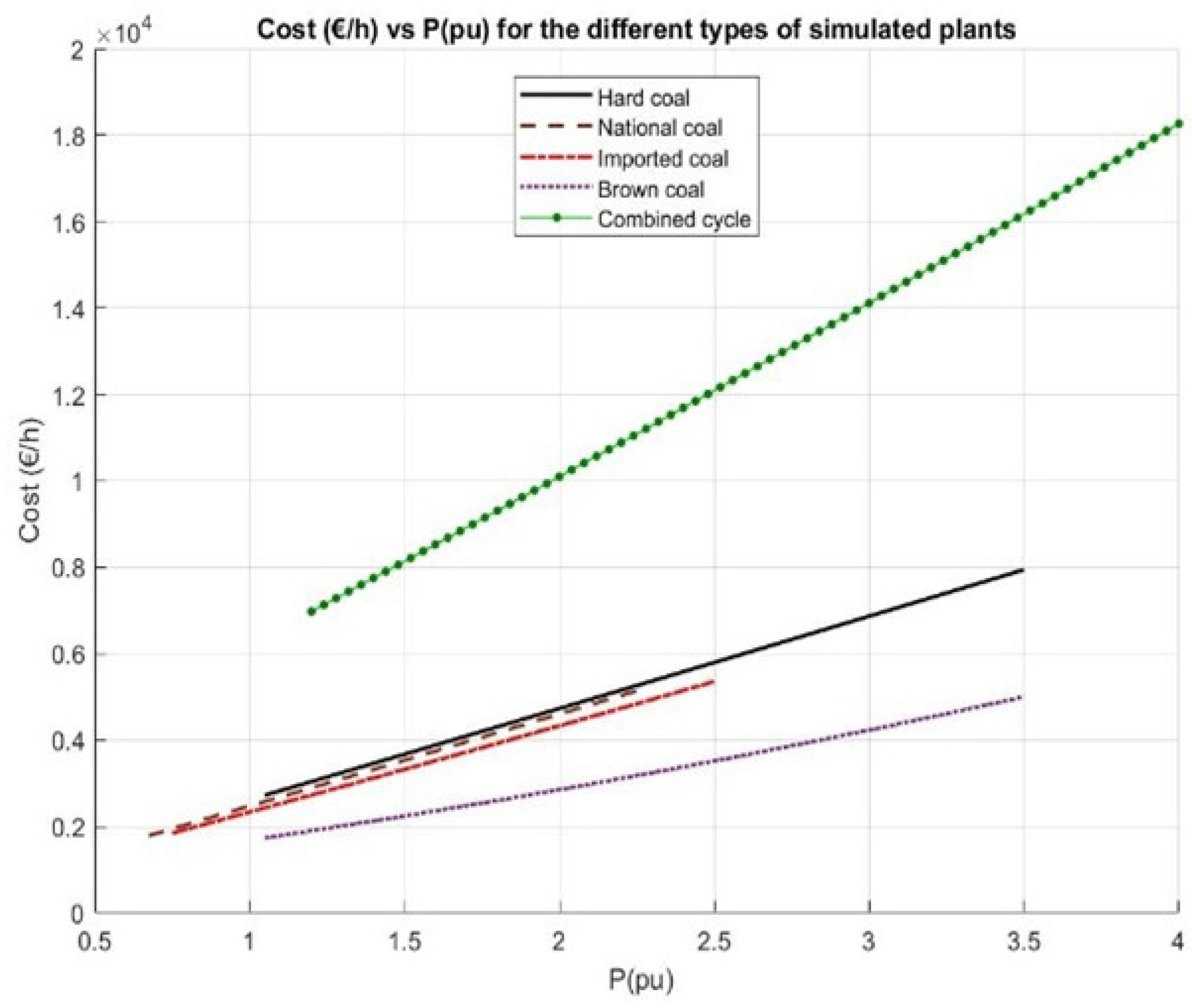
In order to apply the multiobjective optimization model, it is necessary to characterize the thermal generation plants used in the typical network. The cost and emission functions have been determined for brown coal, national and imported bituminous coal, hard coal and combined cycle plants. The most direct way to model the behavior of a thermal group is by adjusting the measurements of the evolution of the magnitude to be studied as a function of the load, and for that several reasonable measurements must be available. Several objectives could be modeled and studied as functions, such as hourly consumption of energy, fuel mass, operating cost, emissions, emissions, emissions and operating cost integrating emissions at the price of the emission allowance.
3.1. Cost Functions
The data necessary to characterize the consumption curves of the power plants are difficult to obtain. To carry out this study, it was consulted a very complete publication of the former Ministry of Industry and Energy (hereinafter MINER) [1], which made available to the general public the marginal consumption, average consumption and start-up costs of each one of the existing plants in 1988. The report classifies the plants by type. Though data may look old, the curves are valid to characterize the behavior of these plants, and they serve well for illustrating the methodology that this paper tries to show.
For the modeling of the combined cycles, a 2x1 cycle with a GE 7FA.04 turbine of 480 MW nominal at 15 °C was analyzed from the data tables of the Bowie plant in Arizona [2].
The hourly energy consumption function is expressed as a function of the heat rate consumption , measured in , and the real power of the power plant:
The fuel consumption is obtained from the energy function, just divided by the lower heating value of the fuel (LHV):
To move to the operating costs function , which is mainly represented by the cost of fuel, you have to multiply by a factor , which is the cost of one kJ of the corresponding fuel:
In general, almost all dispatch or OPF papers [3,4,5,6] model the cost functions according to quadratic polynomial curves:
Lamont and Obessis in [5], use a model according to a cubic, without quadratic term, according to:
Gjengedal et al., in [6], model the cost function as:
In the MINER document [1], in addition to the test data (P, ), the fitting parameters for each plant of the heat rate consumption curves are offered, following a non-linear model and a linear one, according to:
In this study, the first of the two models will be followed for the heat rate of all the plants, giving rise to quadratic polynomial cost curves.
Table 1 shows the characteristics of the fuels and the power plants used.
The heat rate consumption functions of the generation groups classified by type of fuel can be seen in Figure 2A, and Figure 2B shows the associated cost functions.
Figure 3.
Cost Curves, =100 MVA.
3.2. Emissions Functions
emissions come from the fuel, and it can be said that its evolution with power will follow the trend of the fuel consumption curve, multiplied by the per unit mass emission factor of the fuel according to the combustion reaction. That is, if is the per unit content of C in the fuel, deduced from its elemental analysis, and remembering the combustion reactions:
and taking into account the atomic masses of the elements and the molecular masses (: P.M. = 44 g), it will be:
If the carbon retention (unburned) is known, in per unit with respect to the carbon content (C) data of the elemental analysis, the previous function turns into:
4. Multi-Objective Optimization
In multi-objective optimization, multiple functions are involved, usually in conflict one with each other. In this context, in the range of the possible solutions, if you want to improve one of the objective functions by moving to a better solution, another of the objective functions will be penalized or compromised. This commitment rate, which relates the improvement in one objective with the penalty in another, is known in technical literature as “trade off”. There are numerous books, articles, and texts where one can drill down and read about operations research, optimization, and methods or solvers for dealing with optimization problems. To cite some sources, on optimization and operational research in general, the classic by Hillier and Liberman [8], or the one by Chong and Zak [9] can be consulted. There is also a lot of scientific production of specific books on multiobjective optimization, among them, Miettinen k., Deb k. et al [7] or Ehrgott [10]. To begin with, one can get a very good idea of what multiobjective optimization is, the bases and concepts that define it, and the methods and techniques with which it is carried out, by reading the summaries of Marler R. and Arora J. [11], and López Jaimes A. et al [12]. In recent times, research interest in global optimization methods based on genetic and evolutionary algorithms has been intensified, and texts with very good introductions to the theory of multiobjective problems can also be found; it is worth mentioning that of C. A. Coello et al [13], or the thesis of Zitzler E. [14]. The process of systematic and simultaneous optimization of a set of objective functions is called multi-objective optimization (hereinafter MOO), and the problems in which these techniques are applied are called multiobjective optimization problems (hereinafter MOP).
4.1. Definition of a Multiobjective Optimization problem
It will be assumed, without loss of generality, that the problems are in terms of minimization. A maximization problem is equivalent to a minimization problem, since:
A multiobjective problem can be formulated in a generic way as follows:
where:
, is a vector of n independent decisions or design variables, the values of which are to be found in the optimization problem.
, is a vector of m objective functions. Each of the functions components of f are called objectives, criteria or goals.
are each one of the p inequality constraints to which the problem is subject.
are each one of the q equality constraints to which the problem is subject.
The objective function vector f:, is composed of m objective scalar functions and it defines the relationship between the decision or design space , and the space of functions and objectives .
The feasible design space (feasible design space or restricted decision set) is defined as the set X of values in the design or variable space that satisfies the constraints. The set of images of that set will define the Y objective feasible space.
Unlike optimization with a single objective function, with a single solution, in multi-criteria optimization the solution is a set of points that satisfy the optimality concept. In a MOP, the most accepted concept to be able to determine whether a point is optimal or not is that of Pareto optimality or Pareto dominance relationship. This criterion was initially proposed by Francis Ysidro Edgeworth in 1881 [15], but it was formalized and generalized by Vilfredo Pareto in 1896 [16].
In this text, when terminology is used saying that a point improves or betters another point, it means that the first is more optimal than the second, and if it worsens, it means that it is less optimal.
A solution is said to dominate (in the Pareto sense) another vector , if it is true that the point is not worse than in any of the objective functions and, in at least one of them, it improves it.
A vector is said to be a strict Pareto optimal if and only if:
that is, a point is strict Pareto optimal if it is satisfied that there are no other points that improve it in any function without worsening it in at least another function.
The images of strict Pareto optima are situated on the boundary of the objective feasible space. Some MOO algorithms may also produce points very close to this condition, without actually reaching it, and they will also be of interest. Of particular interest are the weak Pareto optimal points, which are those that are not improved by any other point in all functions at the same time, but can be matched in some.
The subset of strict Pareto optimal points within the feasible decision space defines the Pareto optimal set, P*, and the subset of target values of that set is called the Pareto front, PF*.
The Pareto front is located at the most optimal boundary or contour of the objective feasible space, but the set of Pareto optimal solutions does not have to do so in its space. See Figure 4.
There are different methods to find the set of solutions which define the Pareto front. In the case studied, the method has been used.
4.2. Method
This method basically consists of selecting an objective, the most interesting or significant, as an objective function to minimize and treating the rest of the criteria as restrictions, sweeping them between their extreme values. It was introduced by Haimes et al. in 1971 and is discussed in detail in Chankong and Haimes, 1983 [17].
The multiobjective problem posed under the method can be formulated as follows:
With this method all the solutions of the Pareto front can be found, whether convex or not. However, to make a complete and consistent exploration of the contour of interest with the method, the problem must be accessible to certain information: the extremes of the objectives that are to be taken as restrictions must be previously calculated, in order to carry out a sweep of the problem by varying the parameters of the constraints between these limit values. In other words, it must be possible to previously calculate the values min and , obtaining iteratively the minimum of the objective function as the value of is changed progressively from one extreme to the other, increasing it with a suitable step to obtain the desired meshing and distribution.
When the problem is convex and the main objective function is strictly convex, the solutions are strict Pareto optimal. However, when the strict optimality conditions cannot be ensured or demonstrated, and if it is necessary to guarantee that the solutions found are located on the Pareto front, there are mathematical tests to discriminate whether the solutions are in the Pareto front or not ([9] and [18]).
5. Analysis and Modeling of Wind Energy Production Data
The power generated by wind farms depends on the local wind regime where they are located and depends on many factors, giving it a high degree of variability and a complicated prediction. The certainty in estimating the power generated by a wind farm is more complicated as the time horizon of the prediction increases. There are tipìcally energy buying and selling mechanisms and markets in which the energy sale process is carried out 24 hours before it is consumed. This is the case of the MIBEL electricity market, the joint market of Spain and Portugal. This type of market requires the most accurate estimation possible of wind energy production in order to minimize the deviations caused by forecast errors. Although these deviations can be offset by demand deviations, this study will not take into account the relationship between generation and demand deviations.
5.1. Statistical Model
Deviations from scheduled production involve many things like the expected and actual wind speed, the operation of the wind farms or the strategy for generating offers to the market. This means that the distribution of the cited prediction errors does not have to follow usual statistical distributions, such as a normal distribution.
The study aims to see the influence that wind deviations have both on the costs associated with certain emissions levels and on the detail of which conventional power plants must assume such errors. In this study, actual and forecasted wind energy production data from two operational wind farms —Park A and Park B— were used as the foundation for the analysis. Park A has an installed capacity of 13 MW, while Park B operates at a nominal power of 46,6 MW. The dataset includes 9,503 hourly records of planned and actual production for Park A, and 8,760 records for Park B. If deviations are considered as , that is, the difference between programmed and actual wind energy production, Figure 5 and Figure 6 shows the behavior of wind farms A and B and the originated deviations. The normal distribution that best fits the deviation histograms has also been represented in Figure 5 and Figure 6, to see if it would be a good fit. It is observed that the data does not fit well with this distribution, so it is decided to look for different alternatives, the Kernel distribution being the best fitting one.
As a result of the modeling of the deviation histograms, the forecasts in park A are slightly lower on average than the actual generation, and the opposite in park B. Table 2 shows the mean values and standard deviations of both reference parks.
For the statistical modeling of the deviations, it has been decided to use the Kernel statistical distribution, which allows a better fit to the calculated histograms.
This type of distribution smooths the histogram of the data. To do this, each sample is associated with a smoothing function, and the probability density function is generated as a weighted sum of the smoothing functions. If there are n samples available, the probability density estimation can be expressed as:
Where h is the band width, and is the smoothing function, which can range from a square function to a normal, triangular or the Epanechnikov function. The estimation of this distribution has been carried out using the Matlab function "fitdist".
The electrical system under study is a 57-node network with a demand of 1250.8 MW. Reference Wind Farms A and B are too few and too small to have an influence on the network’s behavior. Therefore, it has been decided to scale the data from both wind farms so that they reach an order of 20 % of the total demand to be covered, as well as to generate synthetic data from them that can be used as wind farms at different nodes of the network.
Given that there is not a large amount of available data of foreseen and actual wind powers produced, it was decided to use a statistical distribution model fitting this behavior, and thus to be able to generate a matrix of synthetic deviations as broad as desired. In our case, 2000 wind deviated data were generated for each wind farm. This way, it is possible to study how the solutions of multi-objective optimization, in terms of cost and emissions, vary with respect to the base case, when wind errors are introduced.
To obtain synthetic wind generation data for wind farms with different installed capacities, the following procedure was adopted:
Figure 7.
Reference Bids Selection of Windfarm B.
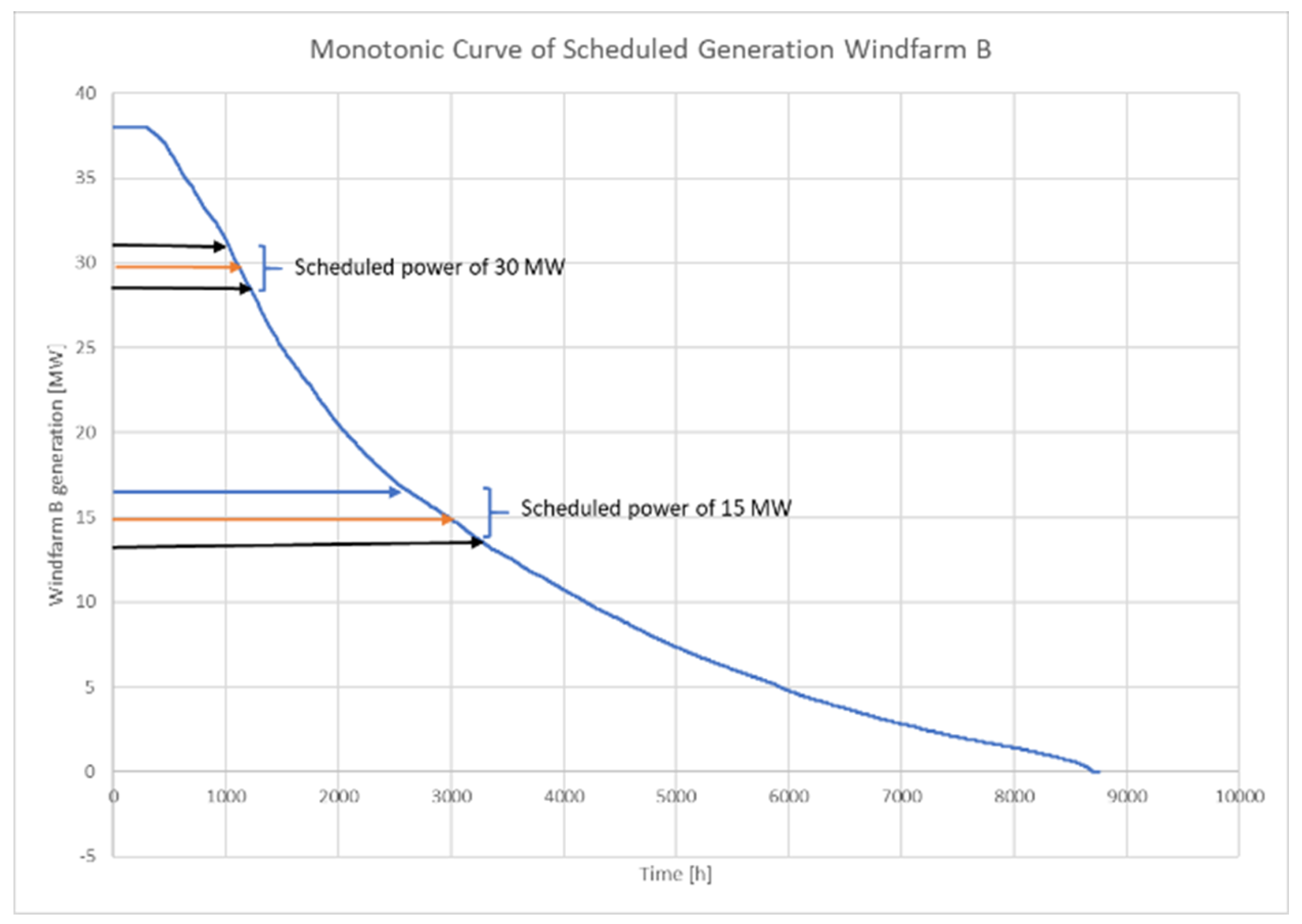
It can be observed how these deviations change from one offer to another, Figure 8 and Figure 9, and do not follow a normal distribution.
To generate an array of actual production values associated with the market bid, the Kernel function that best represents the resulting deviations for each interval has been estimated, based on the actual deviations corrected to the synthetic wind farm’s bid. The prediction error associated with the forecasted offer, , is calculated from the set of deviations associated with the bid bin, scaled to the value of the forecasted offer, :
: Estimate wind power generation in hour h.
: Actual wind power generation in hour h.
: Increment of estimate wind power generation, size of the bin interval.
Both, the powers offered and the deviations originated, have been scaled so that the wind farms have a significant weight, stretching park A from its actual13 MW to a 30.94 MW park and to a 61.1 MW park, and park B from its 46.6 MW to a nominal power of 218.5 MW and a nominal power of 110.67 MW.
The estimation of the Kernel distributions, which are the best fitting the histograms of the offers deviations, where carried out in Matlab. Later, arrays of random deviations were generated following the Kernel distributions associated with each offer, Figure 10.
The adjustment of the kernel distributions of the offers gives the result of Table 3.
In Figure 11, Figure 12 and Figure 13 it can be seen the adjustment of the deviations for the offers 16.66 MW, 70.5 MW y 71.4 MW studied.
Finally, random arrays of actual productions are generated for the different market bids in order to simulate the different scenarios.
6. Approach to the Multiobjective Optimization Model
Before describing how the multiobjective optimization problem is formulated, it is necessary to detail the formulation of the optimal load flow problem in which we want to minimize a single objective function , subject to the constraints of power balance at the buses, power transportation capacity limits for the transmission lines and admissible voltage and generated powers values.
First, the formulation of a single objective problem f(x) is first recalled, generically:
Particularizing it to our purpose, and writing it in the nomenclature of the variables of an electrical power system:
where,
and where
are the number of nodes (or buses) in the system, the number of generation nodes, and the number of branches or connections between buses.
ic is an array ( x 2), which contains the starting and ending positions of the branches of the network.
is the number of functions for which the system has been characterized. In a single target OPF, only one of them is minimized.
, are the modulus of the power flow in the branch between nodes j-k, and the transport capacity of that branch.
, are the complex voltages, their modulus and their angle, at each bus.
, are the active and reactive powers generated at the buses.
, are the active and reactive powers demanded at the buses.
, are the off-diagonal and diagonal terms of the network admittance matrix.
, are the series and parallel admittances of the pi diagram of the connection lines between buses j and k of the electrical system.
, introduces the possibility of considering the existence of regulating transformers in the lines; the normal case, a simple line, has no regulating transformer, and in that case is the real unit.
The system in which it was carried out the study is the network of the IEEE-57 case, a network with 57 buses, 80 lines, and a demand of 1250.8 MW. Figure 14 indicates the location of the thermal power plants, the location of the main loads is depicted with circles and wind power plants with rectangles.
In the simulation of this paper, wind generation situations have been introduced in six nodes of the network, in the igw nodes: 17, 38, 7, 10, 29, 15, simulating as a basis the scene of the offered generation, [MW] = [16.66, 28.56, 32.9, 56.4, 70.5, 71.4], a total amount of 276,42 MW of wind power. Subsequently all the study will deal with the different registered situations of actual powers deviated from that offer.
To introduce the generation of wind power in these nodes, an additional condition is added to the previous algorithm:
where is the number of nodes with wind generation in the system (in this article, =6).
is a vector (1 x ), which contains the positions of the nodes with wind generation.
In this way, the generation of wind energy is simulated as a negative demand in the corresponding nodes, and it is always accepted by the network, whatever the situation of the electrical variables or the rest of the generation of the system.
Once seen the formulation of an OPF, it is possible to proceed to propose a multi-objective optimization, for two functions, =2, in the case of this article, the costs and the emissions functions. To apply the method, explained above, the first thing to do is to calculate the maximum and minimum of the studied functions. The pseudo code to do this is shown below, to do it with the k handled functions:
Thus, the minimum values and maximum values of the functions will be stored in the matrix of dimensions ( x 2).
With the previous values, the objective functions are normalized, because otherwise the difference in the magnitudes, and not their importance, can condition the optimization. Thus, the new normalized objectives will be:
With this normalization, the objective functions are bounded between 0 and 1.
Once the functions have been normalized, the multiobjective optimization of the two chosen functions can now be carried out. The pseudo code of the algorithm to do this, sweeping (n+1) points, shall be written:
where , are the optimal values found in each iteration for the variables, and for the two functions . All information provided by the solver itself and deemed appropriate, such as information on convergence, will also be stored.
In order not to extend this writing further, it will not be detailed here, but the solutions found were subjected to a filter to eliminate dominated points that may have been produced, and to a strict optimality test.
7. Simulation Analysis
To carry out the simulation, the first task was to calculate the extreme values for the cost and emissions functions of the system, and the Pareto front for the forecast powers of the wind farms commented before.
When exploring the extreme values of the objective functions, the system is capable of meeting demand through a range of generation mixes, resulting in cost values between 28,976 €/h and 39,546 €/h, and CO2 emissions ranging from 640,.59 t/h to 945.12 t/h. Figure 15 displays the multi-objective frontier without filtering out dominated solutions, allowing the visualization of the boundary values for the emissions function. The four points located in the bottom-right corner are not part of the Pareto front, as each can be outperformed by other solutions that offer both lower cost and lower emissions. These points are therefore considered dominated. Nevertheless, the rightmost point represents the highest level of CO2 emissions the system can produce—945.12 t/h—which is taken as the upper bound for emissions.
The Pareto front establishes the base case upon which to analyze how the optimal solutions vary when the actual power injected by the wind farms differs from the forecast.
For each estimated windfarm, a series of 2000 points of random power deviations have been generated following the Kernel distributions adjusted in the previous section. Thus, 2000 random combinations of the six wind farms powers, deviated from the estimated forecast, were generated. The combinations that represented the maximum increase (Max-Wind) and decrease (Min-Wind) of total wind over the forecast were identified.
Figure 16 shows the Pareto fronts, between the cost and CO2 emissions functions, for four significant situations: maximum wind, forecast wind, minimum wind and null wind. The ranges of costs and emissions along which the functions move, change for each situation, increasing as the wind decreases, since wind can be interpreted as a decrease in demand at zero cost.
Next, taking the estimated wind forecast curve as a base, they were sought the solutions that provide the optimal generation cost for the 2000 combinations of wind farm deviations, with the restriction of complying with a determined amount of global emissions in the system. The simulations were carried out to comply with 25 %, 50 % and 75 % of the emissions interval found in the base case, id est, to comply with an emission objective of 717 t/h, 793 t/h and 869 t/h respectively. A total of 6,000 situations (2,000 for each emission limit) were simulated and solved.
In Figure 17, the evolution of the Pareto Front base is observed in a continuous curve, and the vertical dispersion of points indicates the optimal cost complying with a determined constraint of generated emissions for all the random wind deviations studied. Each vertical dispersion group of solutions contains around 2,000 points, actually slightly less, because non acceptable solutions in relation to optimality convergence were discarded.
As an example, Figure 18 shows how the Pareto front changes as the wind deviates. The upper curve in the figure is the Pareto front for one of the 2,000 random Kernel deviations, in this case for a situation accounting for a total wind power decrease of 139 MW. In the figure, the circles indicate the new optimum solutions for the system to still respect the 25 %, 50 %, and 75 % of the emissions range.
The important fact is that it is possible to identify for any deviation the new optimal solutions for the system, satisfying any emission limit wanted, and so, it is possible to take correction actions, for the short term dispatch strategy or for the intraday or secondary markets offers.
Figure 19 and Figure 20 show an example of how the thermal generation mix changes to adjust emissions and how increased environmental restrictions lead to the substitution of coal for natural gas.
The introduction of variable wind generation means that the conventional generation mix that fits the expected emissions at an optimal cost has to change due to the cited prediction error of the wind power. This effect can be observed in Figure 19 and Figure 20, where the points of optimal costs have been calculated for emissions adjusted to the 0.25 pu and 0.75 pu of the emissions range, considering the variability in wind generation. The generation mix is also represented for the cases of maximum and minimum cost.
For both the emission limits of 0.25 pu and 0.75 pu, it is the combined cycle that must assume a greater variability. In the solution corresponding to 0.75 pu of the emissions, the national coal and brown coal plants can help the system to compensate for wind deviation. This same effect is observed to a lesser extent in the case of limiting emissions to 0.5 pu. Another factor to consider is the location of wind power generation and conventional power plants within the electrical network under study, because the limitations in the transmission of energy can vary the power that each plant must contribute to compensate for the wind deflections.
Finally it is also possible to study and represent how the total optimal cost changes with the wind power deviations, while maintaining a certain level of emissions, as shown in Figure 21 for a 50 % of the emissions range of the baseline case.
The distribution of optimal costs around the value obtained in the base case, associated with the studied emissions, indicates that the mix of forecast errors committed in the wind farms studied has a strong influence and that it does not follow a homogeneous distribution around the value of the base case, as expected.
The results of the simulations (see Table 4 indicate that the average cost of the actual powers is higher than the Pareto estimated cost, which indicates that the existing asymmetries in the forecast errors originate an average extra cost of the order of 2.68 % in the case of emissions at 0.25. pu. Figure 22 shows a summary of the histograms of the incremental costs and it can be seen how the wind forecast errors are echoed to the generation costs. The variability of costs with respect to the base case follows different distributions depending on the emissions restriction.
For a 25 % emission restriction, costs are increased because it is the combined cycle that assumes practically all the wind diversions to be reduced. In the case of the 50 % restriction on emissions, costs fall as more thermal generation enters, which allows the cycle to have to assume less generation to rise. The case of the 75 % emission limit follows an atypical cost histogram because the excesses of wind generation are assumed by the national coal and brown coal plants.
8. Conclusions
The progressive increase in renewable energies in the electricity system implies an improvement from the environmental point of view, as well as a decrease in the degree of energy dependence of the countries. It makes society more sustainable and cleaner, but we must not forget that in order to meet environmental objectives, it is also necessary to deal with the particularities of each renewable system. The uncertainty associated with wind and solar energy, which are, on the other hand, the pillars of the change in the electricity generation system, make it necessary to study the impact that these energies originate both in the operation of the electricity system, as well as in the extra costs associated with that operation.
Throughout the study, a calculation procedure is identified that can help to see the effect of wind variability in the decision-making in conventional thermal generation. In the multiobjective optimization, an AC OPF has been programmed. Also, it has been seen that, with the available data, there is not a homogeneous distribution of the prediction errors around the predicted value. This may be due to deficiencies in the prediction and to the parks operation influence. The statistical modeling of the prediction errors from kernel distributions allows the generation of random values fitting optimally the calculated histograms.
In this initial study, only thermal generation plants have been considered. In the future, hydraulic generation and energy storage systems will be incorporated into optimization, such as batteries, compressed air or hydrogen storage, that shall significantly modify how the electrical system is managed.
Funding
This research received no external funding.
Conflicts of Interest
The authors declare no conflicts of interest.
References
- Ministerio de industria y Energía. Delegación del gobierno en la explotación del sistema eléctrico, «Las centrales termoeléctricas. Consumos marginales, consumos medios y costes de arranque.», 1st ed.; Publisher: Madrid, Spain, 1988. [Google Scholar]
- Arizona Department of Environmental Quality. ADEQ. Air Quality Division: Permits: Bowie Power Station. Available online: https://www.azdeq.gov/environ/air/permits/bowiepowerstation.html (accessed on October 2015).
- AlRashidi, M.; El-Hawary, M. Emission-economic dispatch using a novel constraint handling particle swarm optimization strategy. In Proceedings of the Canadian Conference on Electrical and Computer Engineering (CCECE ’06), Ottawa, Canada; 2006. [Google Scholar]
- Wu, L.; Wang, Y.; Yuan, X.; Zhou, S. Environmental/economic power dispatch problem using multi-objective differential evolution algorithm. Electric Power Systems Research 2010, 80, 1171–1181. [Google Scholar] [CrossRef]
- Lamont, J.; Obessis, E. Emission dispatch models and algorithms for the 1990’s. IEEE Transactions on Power Systems 1995, 10(2). [Google Scholar] [CrossRef]
- Gjengedal, T.; Johansen, S.; Hansen, O. A qualitative approach to economic environmental dispatch. Treatment of multiple pollutants. IEEE Transactions on Energy Conversion 1992, 7(3). [Google Scholar] [CrossRef]
- Branke, J.; Deb, K.; Miettinen, K.; Slowinski, R. Multiobjective Optimization. Interactive and Evolutionary Approaches; Springer-Verlag: Berlin-Heidelberg, Germany, 2008. [Google Scholar]
- Hillier, F.; Lieberman, G. Investigación de operaciones, 9ª ed.; McGraw-Hill: México D.F., México, 2010. [Google Scholar]
- Chong, E.K.; Zak, S.H. An Introduction to Optimization; John Wiley & Sons: New Jersey, USA, 2008. [Google Scholar]
- Ehrgott, M. Multicriteria Optimization; Springer: Heidelberg, Germany, 2005. [Google Scholar]
- Marler, R.; Arora, J. Survey of multi-objective optimization methods for engineering. Struct. Multidisc. Optim. 2004, 26, 365–395. [Google Scholar] [CrossRef]
- Jaimes, A.; Martínez, S.Z.; Coello, C.C. An introduction to multiobjective optimization techniques. In Optimization in Polymer Processing, 2011; pp. 1–26.
- Coello, C.; Lamont, G.; Veldhuizen, D.V. Evolutionary Algorithms for Solving Multiobjective Problems; Springer: New York, USA, 2007. [Google Scholar]
- Zitzler, E. Evolutionary Algorithms for Multiobjective Optimization: Methods and Applications. Ph.D. Thesis, Swiss Federal Institute of Technology Zurich, 1999.
- Edgeworth, F. Mathematical Physics; P. Keagan, 1881.
- Pareto, V. Cours d’économie politique; F. Rouge, 1896.
- Chankong, V.; Haimes, Y. Multiobjective Decision Making: Theory and Methodology; Elsevier Science Publishing: New York, USA, 1983. [Google Scholar]
- Berizzi, A.; Bovo, C.; Innorta, M.; Marannino, P. Multiobjective optimization techniques applied to modern power systems. In Proceedings of the IEEE Power Engineering Society Winter Meeting, Columbus, OH, USA; 2001; Volume 3. [Google Scholar]
Figure 1.
Computation Procedure.
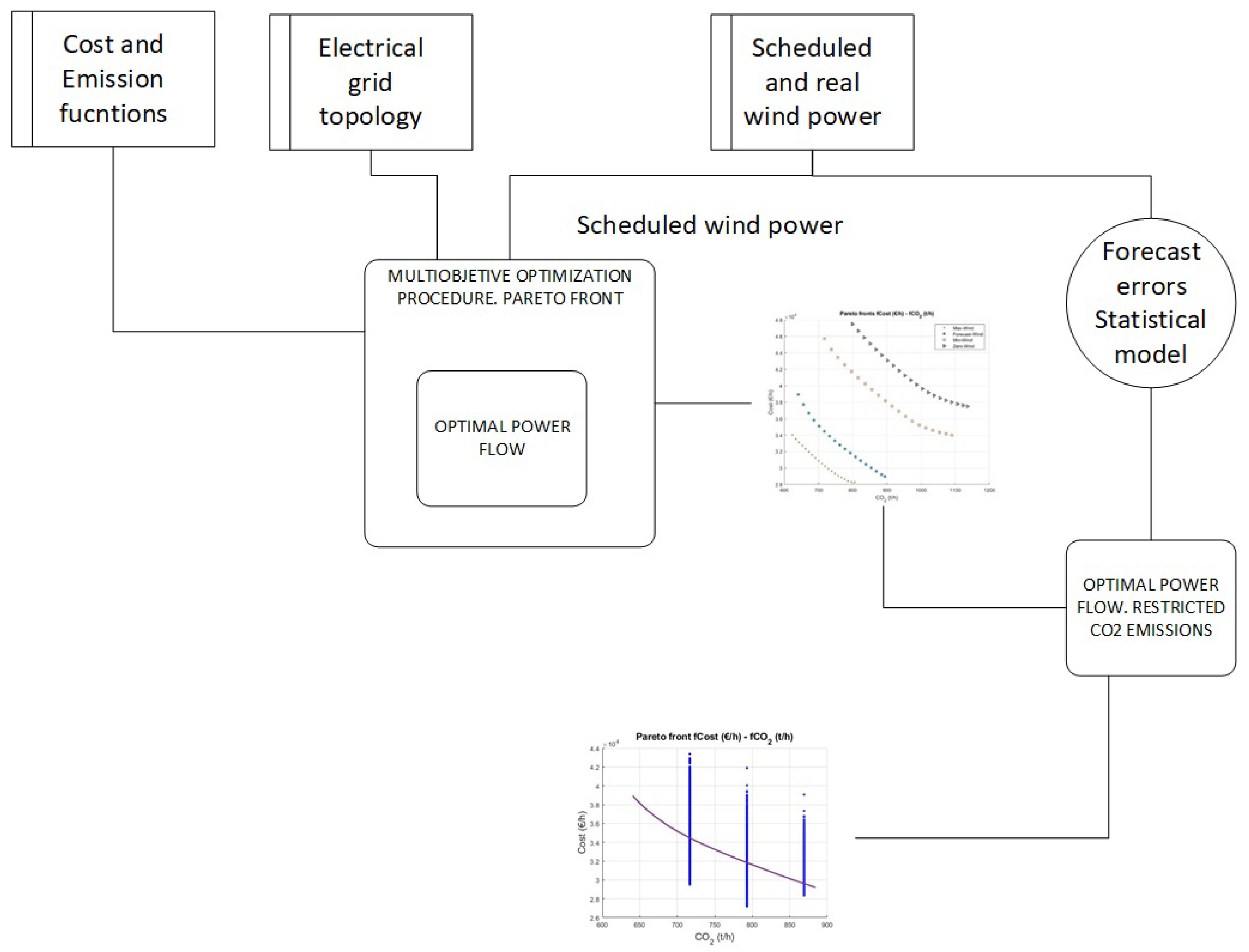
Figure 2.
Heat Rate Curves.
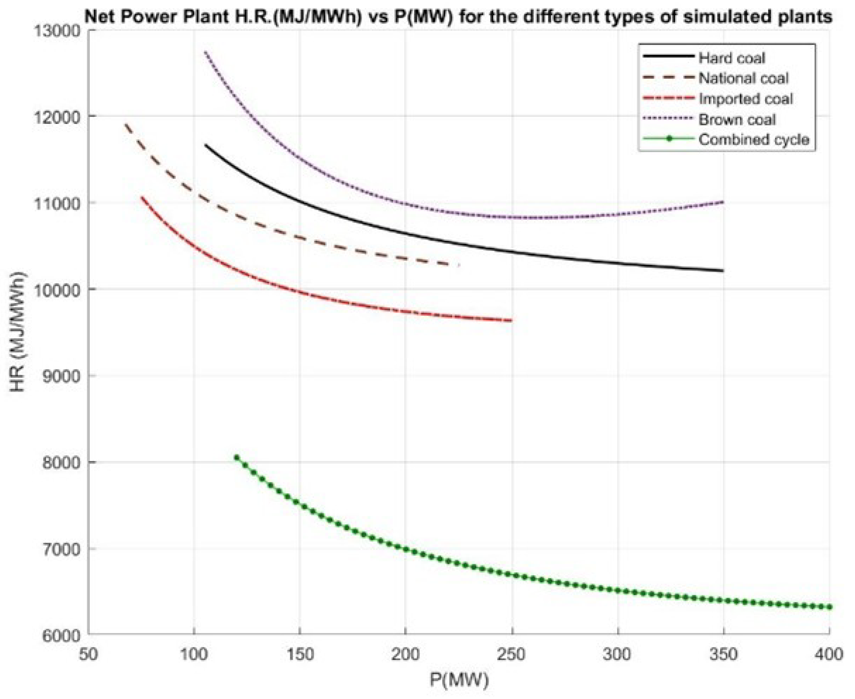
Figure 4.
Pareto Optimal Set and Pareto Front.
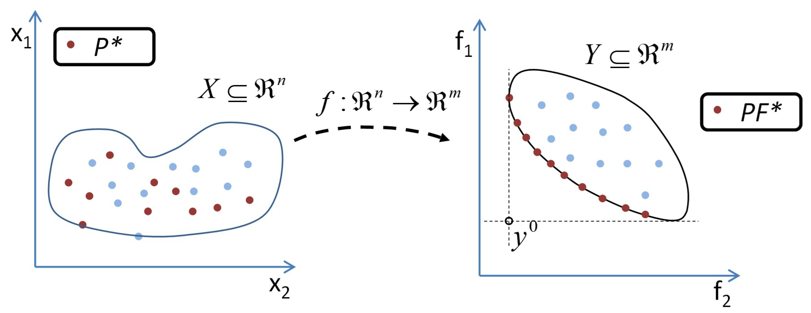
Figure 5.
Comparation Between Histogram of Deviation versus Normal Distribution in Windfarm A.
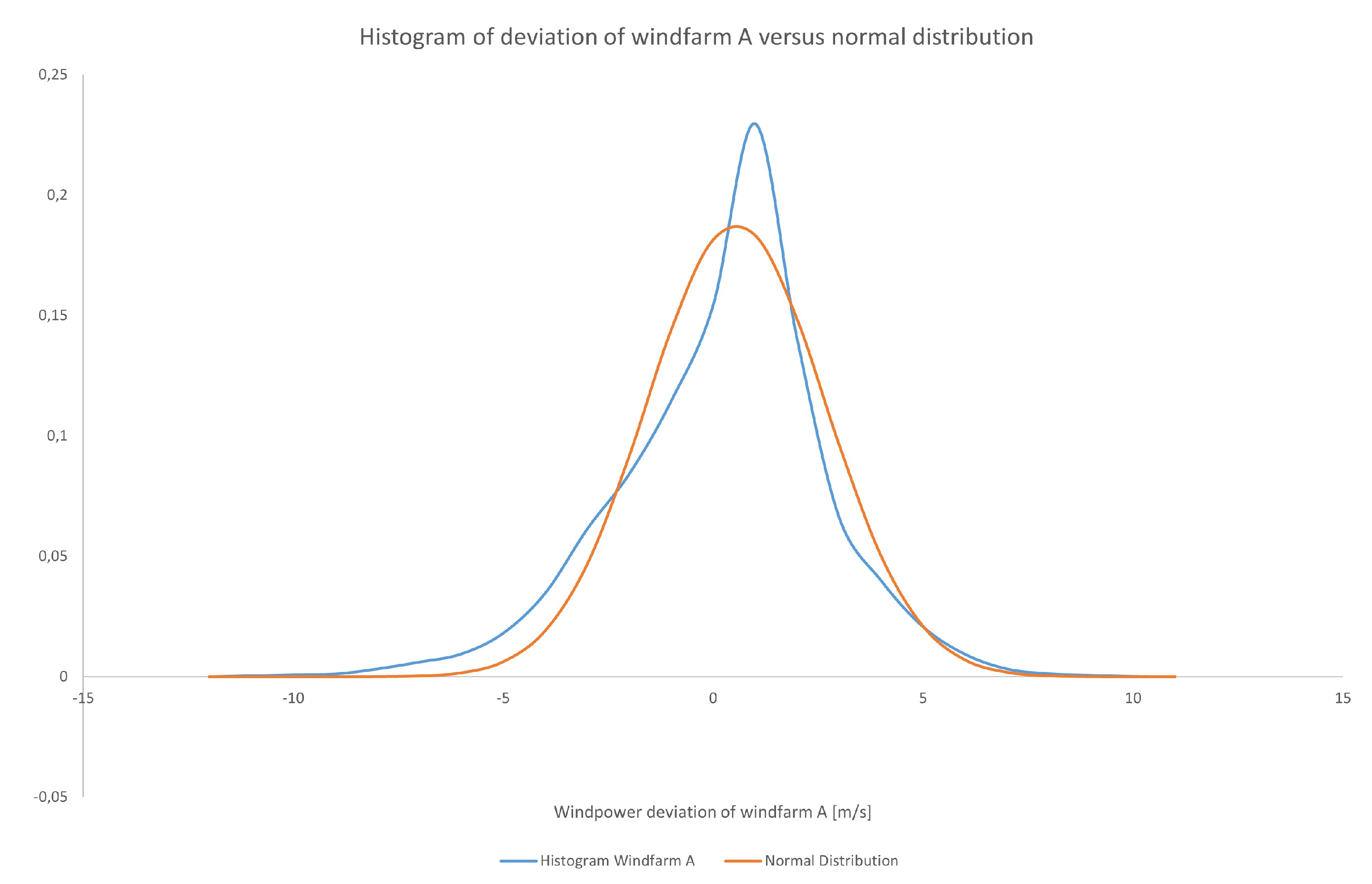
Figure 6.
Comparation Between Histogram of Deviation versus Normal Distribution in Windfarm B.
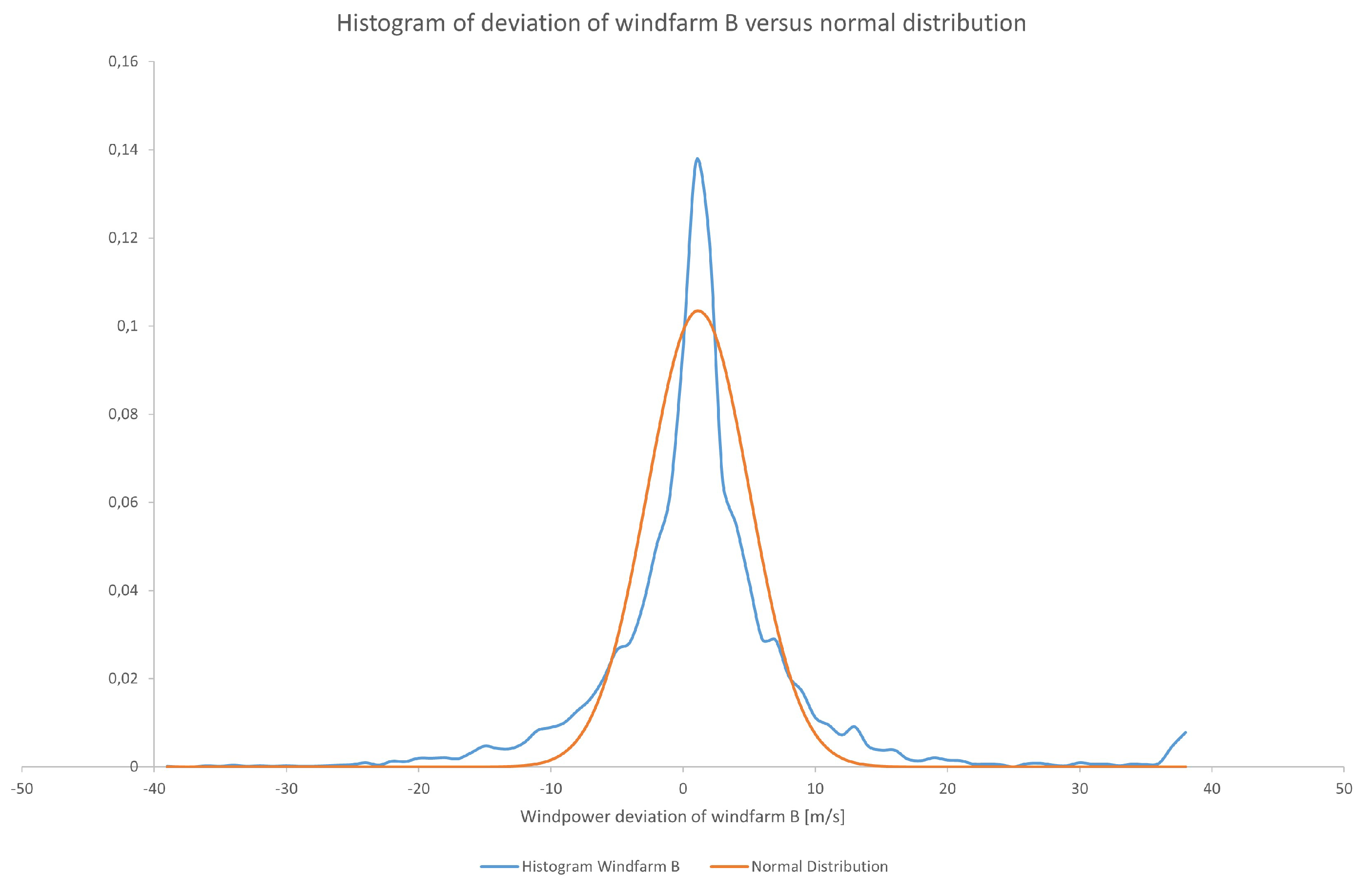
Figure 8.
Power Deviation Histogram for a Bid of 15 MW of Windfarm B.
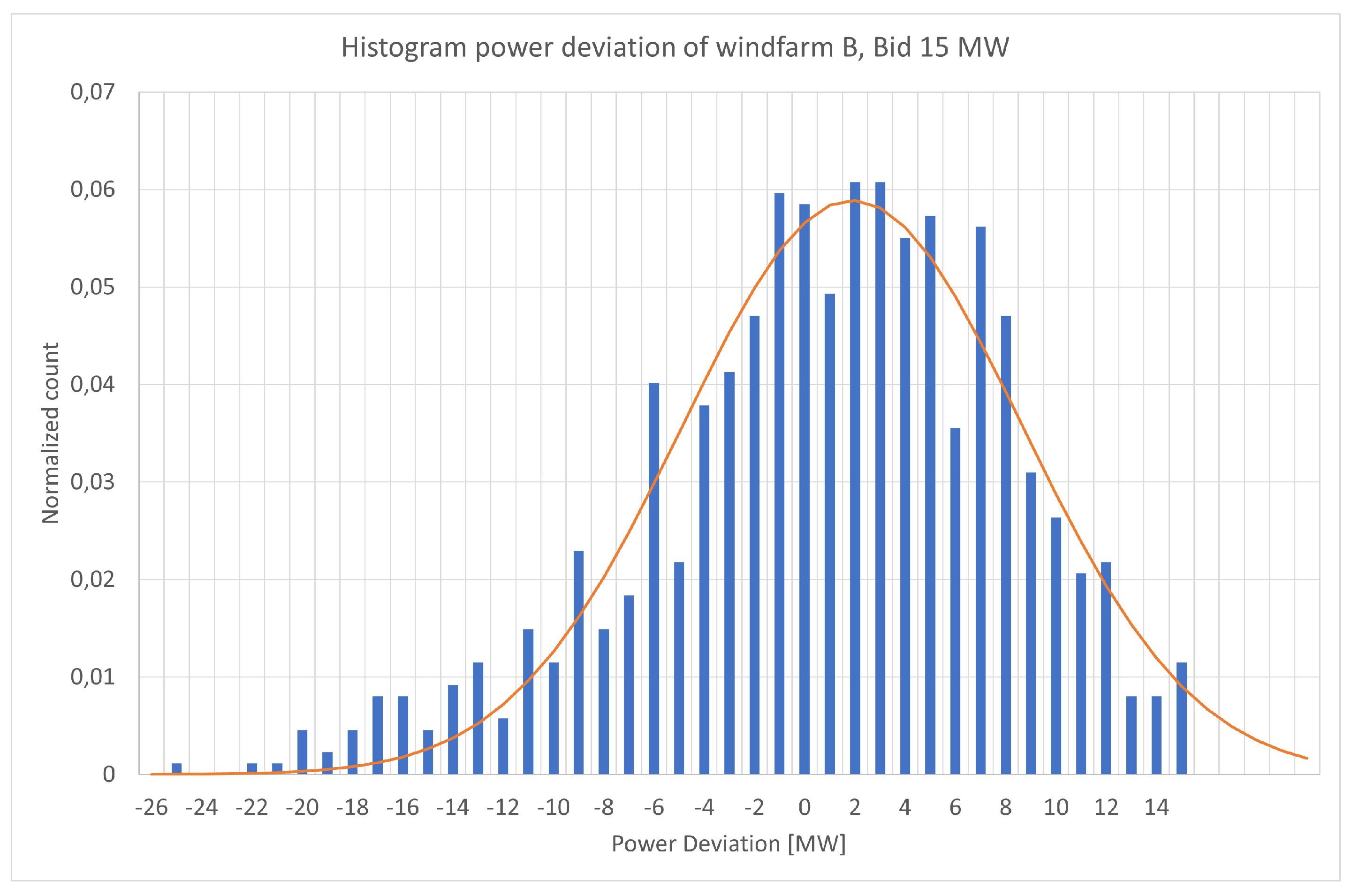
Figure 9.
Power Deviation Histogram for a Bid of 30 MW of Windfarm B.
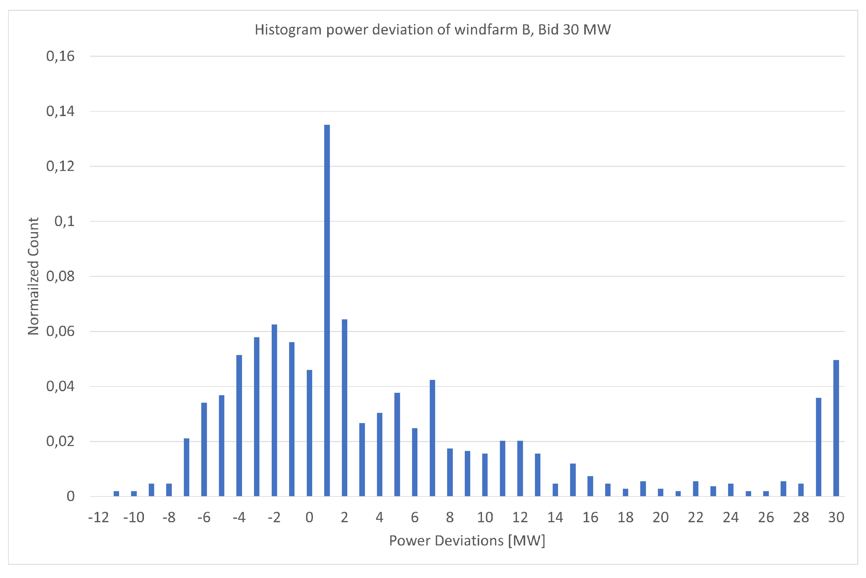
Figure 10.
Bid and Actual Generation of Windfarm A.
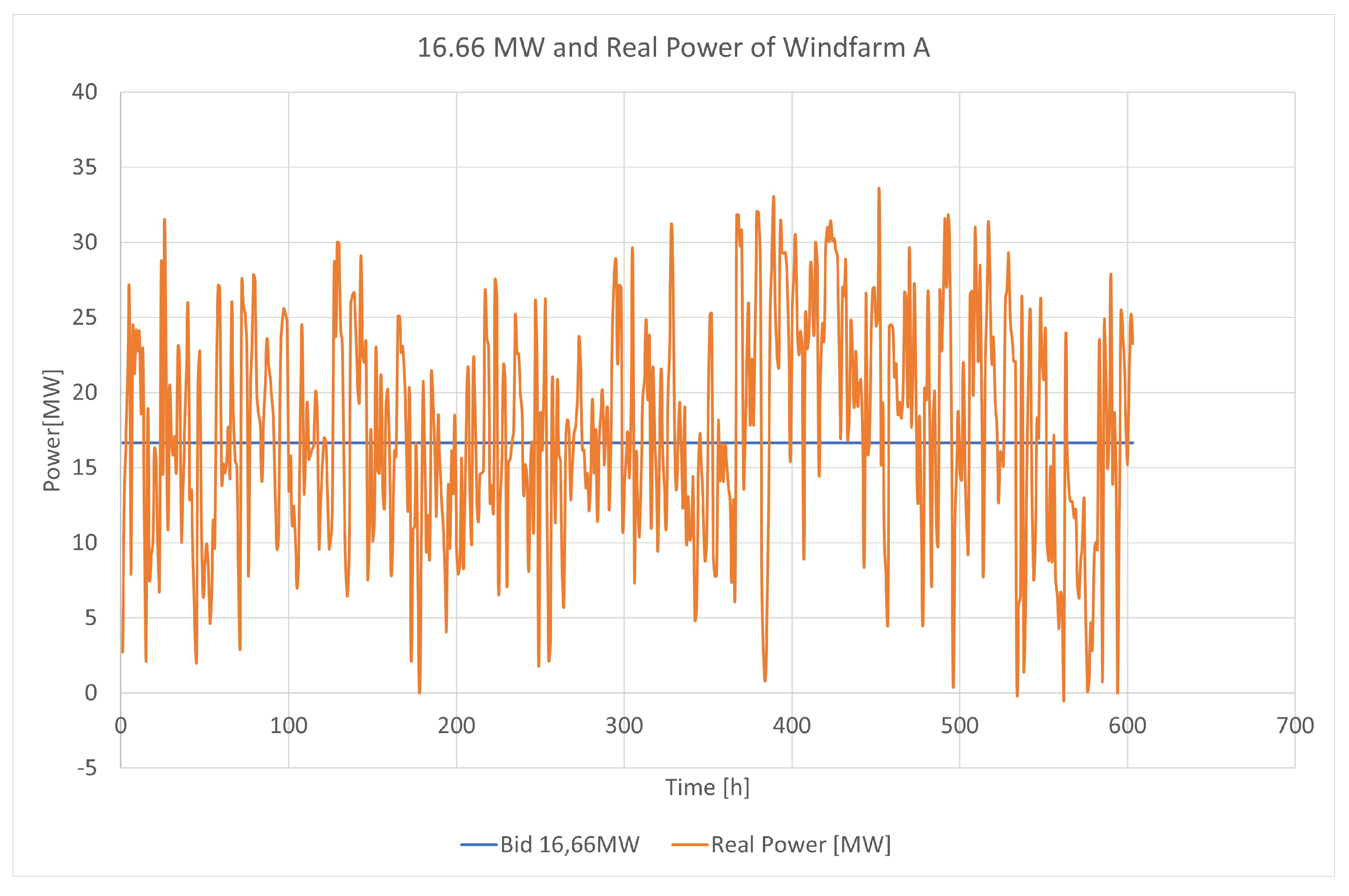
Figure 11.
Kernel Distribution Estimation 16.66 MW.
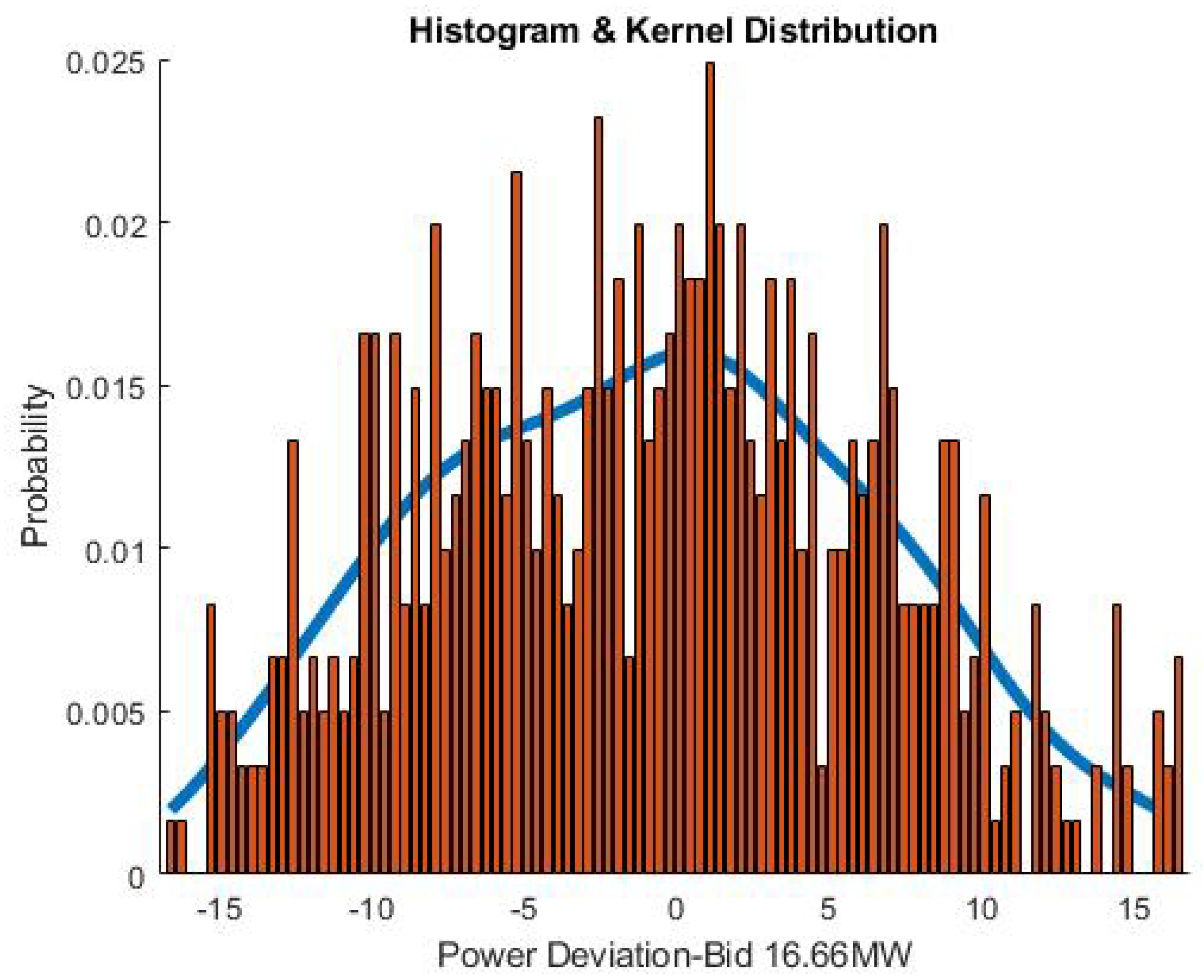
Figure 12.
Kernel Distribution Estimation 70.5 MW.
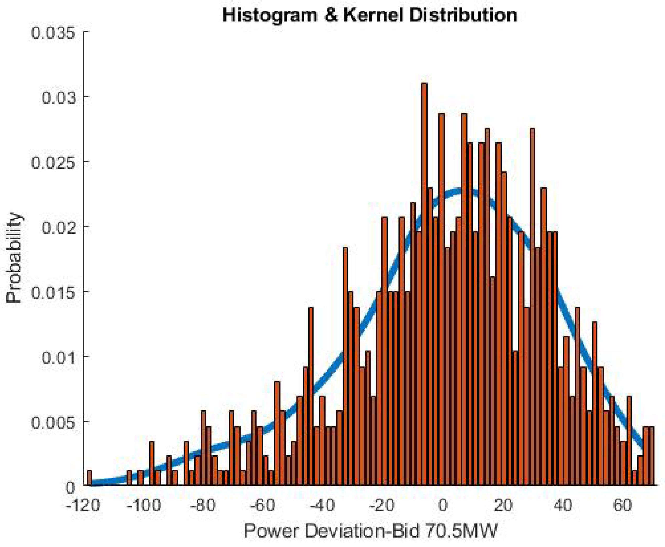
Figure 13.
Kernel Distribution Estimation 71.4 MW.
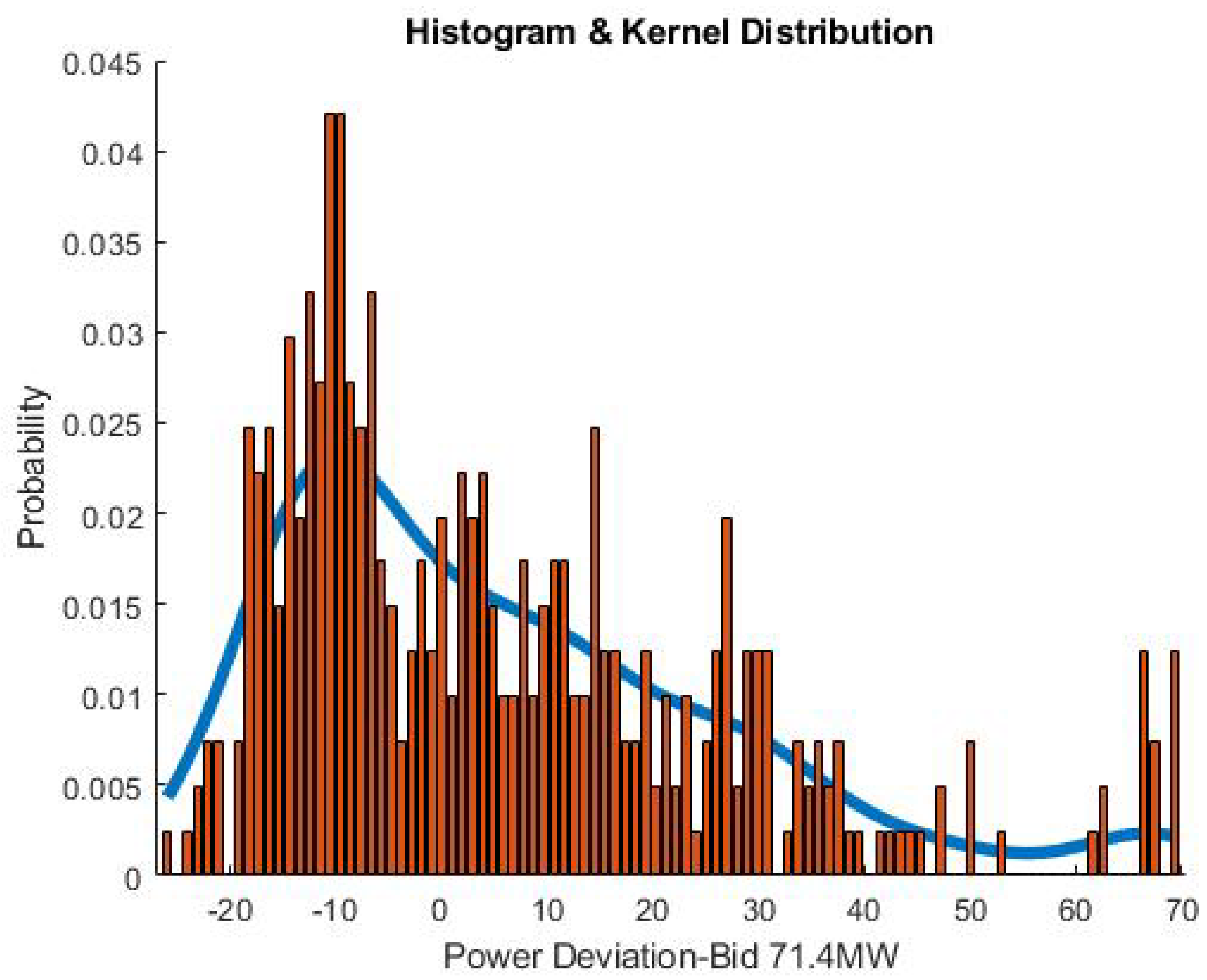
Figure 14.
: IEEE-57 Electrical System with Thermal Power Plants AND Windfarms indicated.
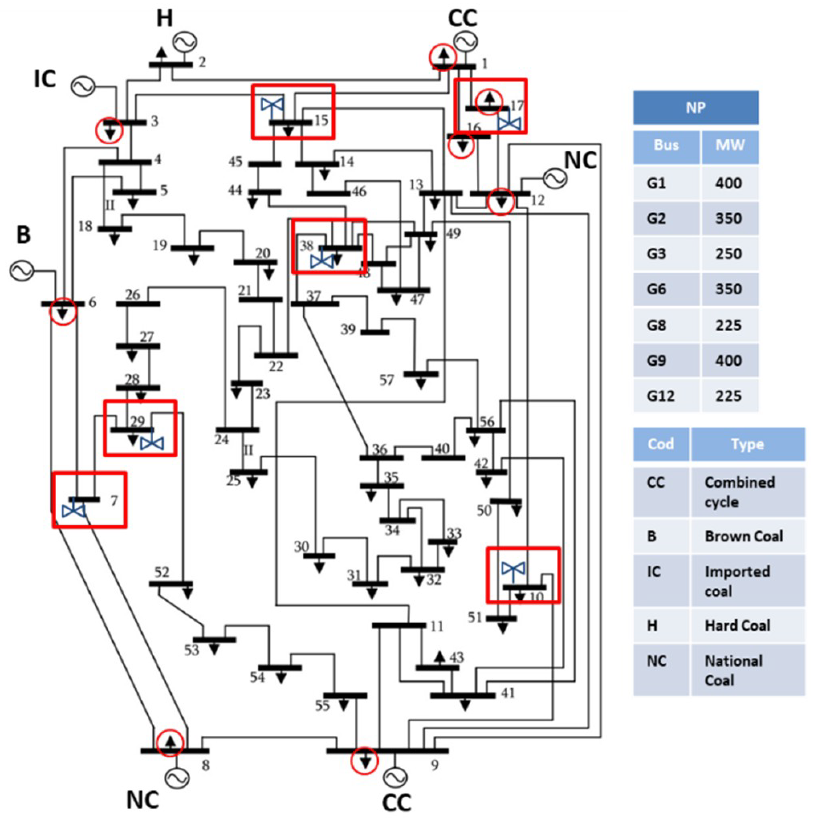
Figure 15.
: Multiobjective front without filtering dominated points showing the system CO2 emissions boundaries.
Figure 15.
: Multiobjective front without filtering dominated points showing the system CO2 emissions boundaries.
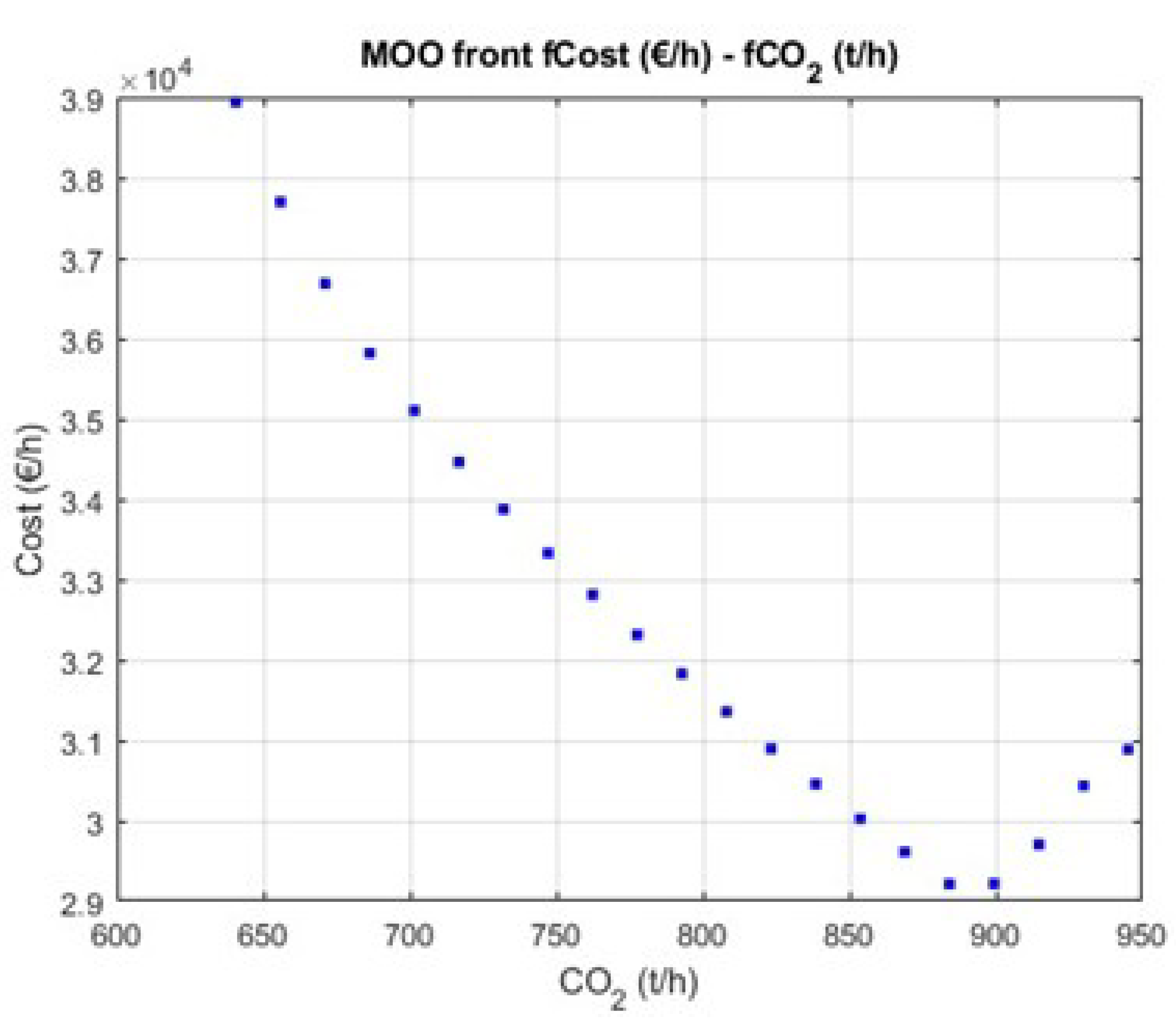
Figure 16.
: Pareto fronts in four different significant possible wind situations.
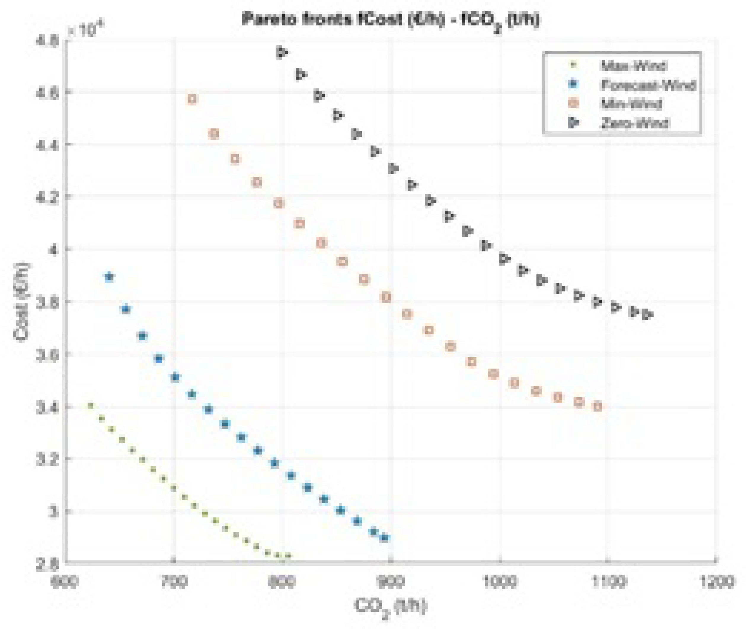
Figure 17.
: Base case Pareto front and new optimum cost solutions for the 2000 wind Kernel deviations, when respecting the 25 %, 50 % and 75 % of the emissions range.
Figure 17.
: Base case Pareto front and new optimum cost solutions for the 2000 wind Kernel deviations, when respecting the 25 %, 50 % and 75 % of the emissions range.
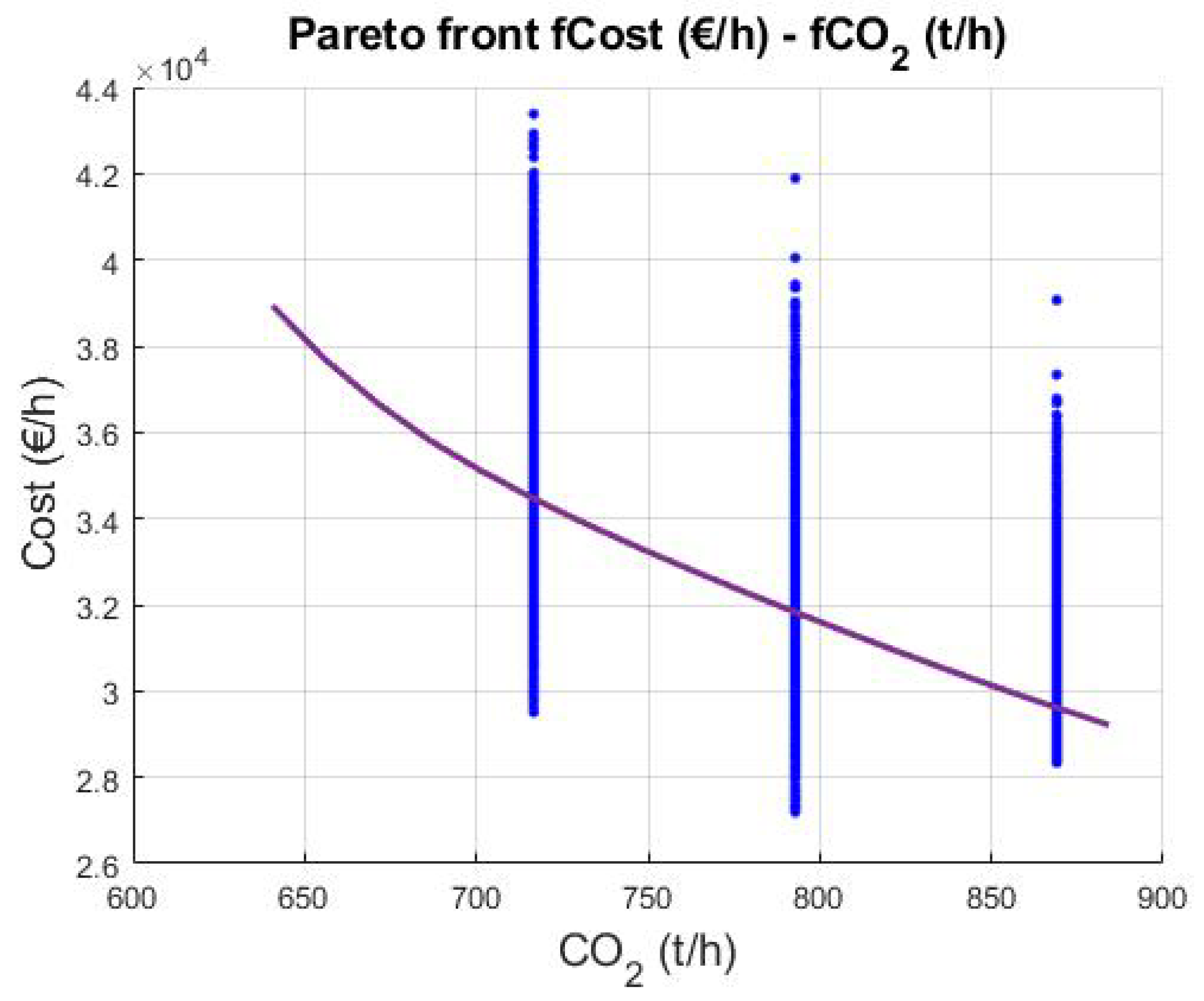
Figure 18.
: New Pareto front above the baseline for a 139 wind power decrease and identification of new solutions respecting 25 %, 50 %, and 75 % of the emissions range.
Figure 18.
: New Pareto front above the baseline for a 139 wind power decrease and identification of new solutions respecting 25 %, 50 %, and 75 % of the emissions range.
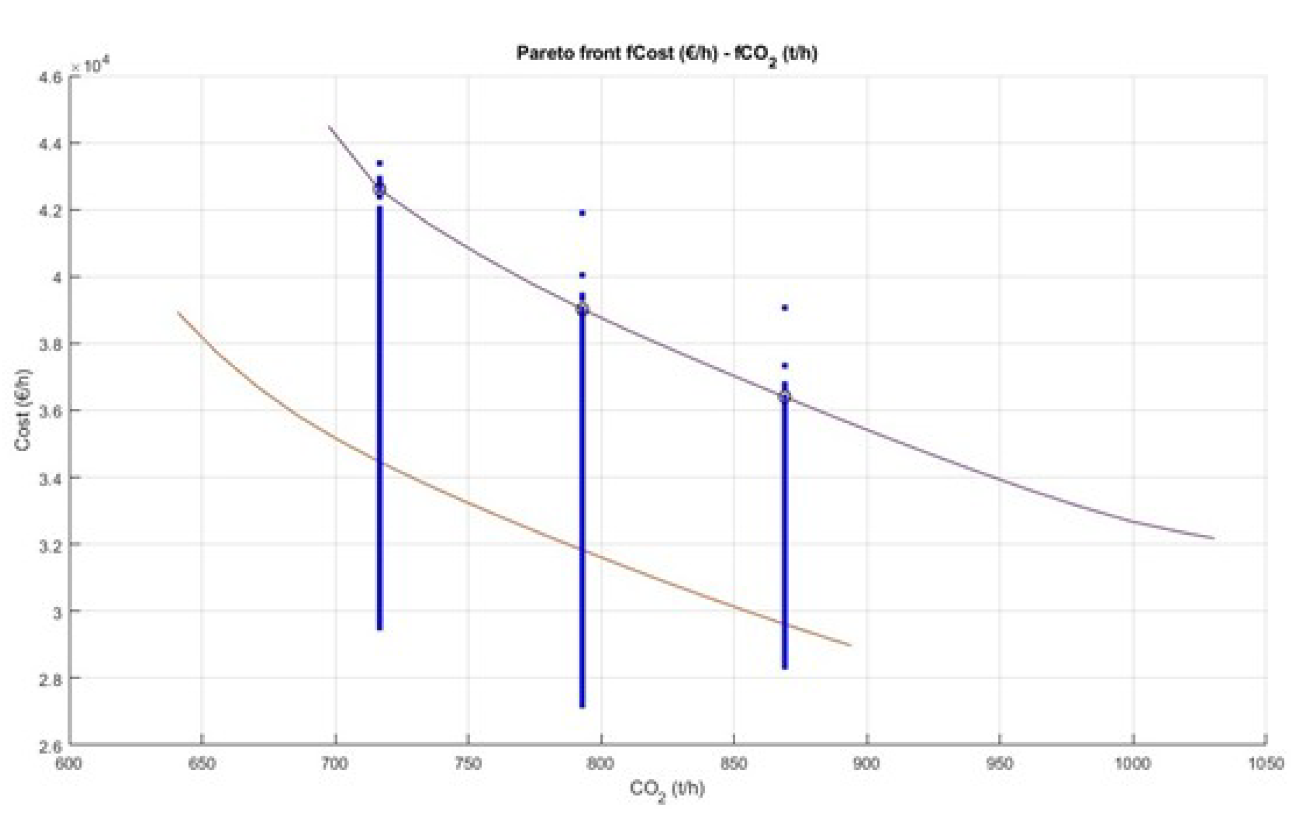
Figure 19.
: Generation Mix Solution for 0.75 pu Emission Limitations.
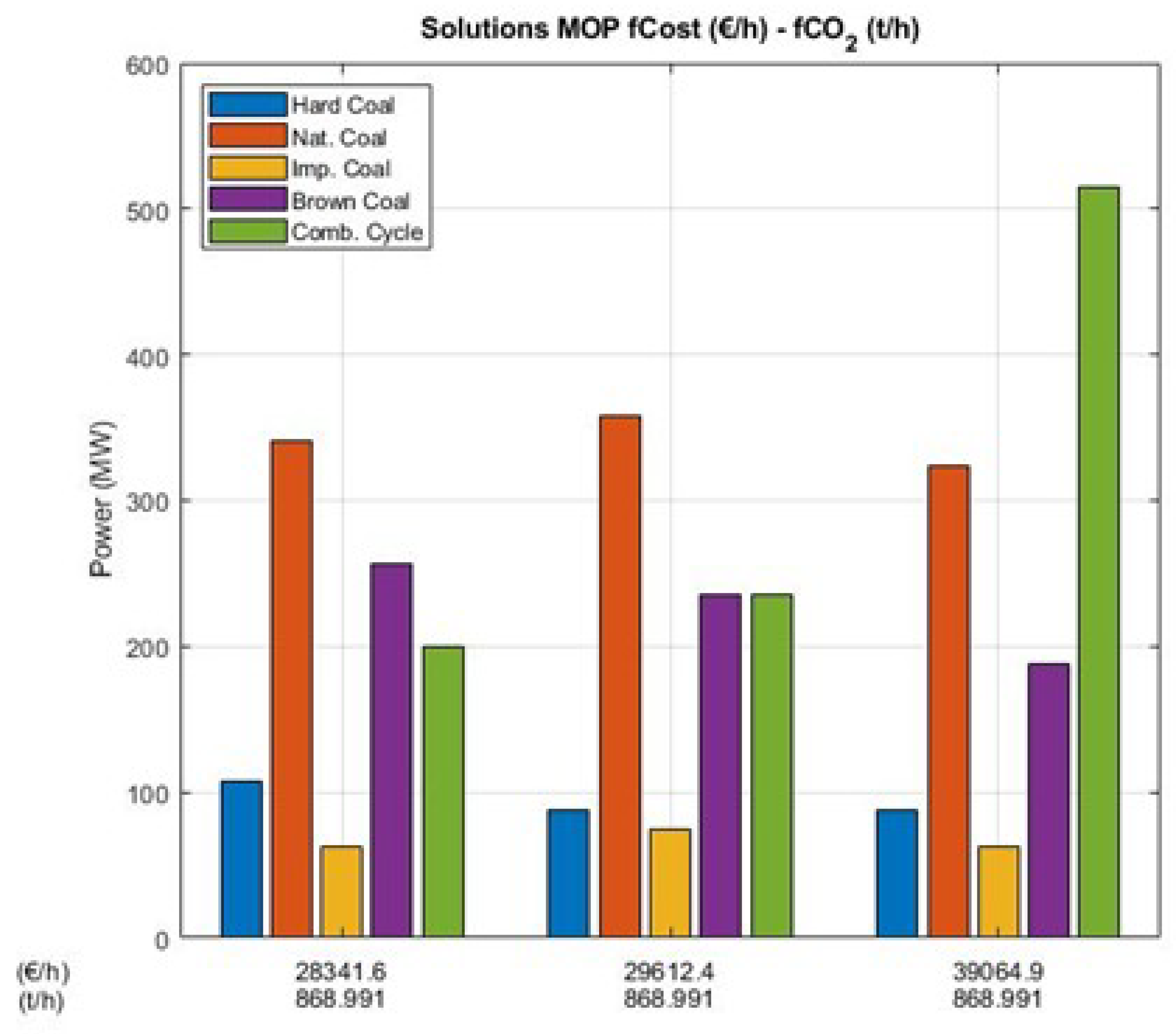
Figure 20.
: Generation Mix Solution for 0.25 pu Emission Limitations.
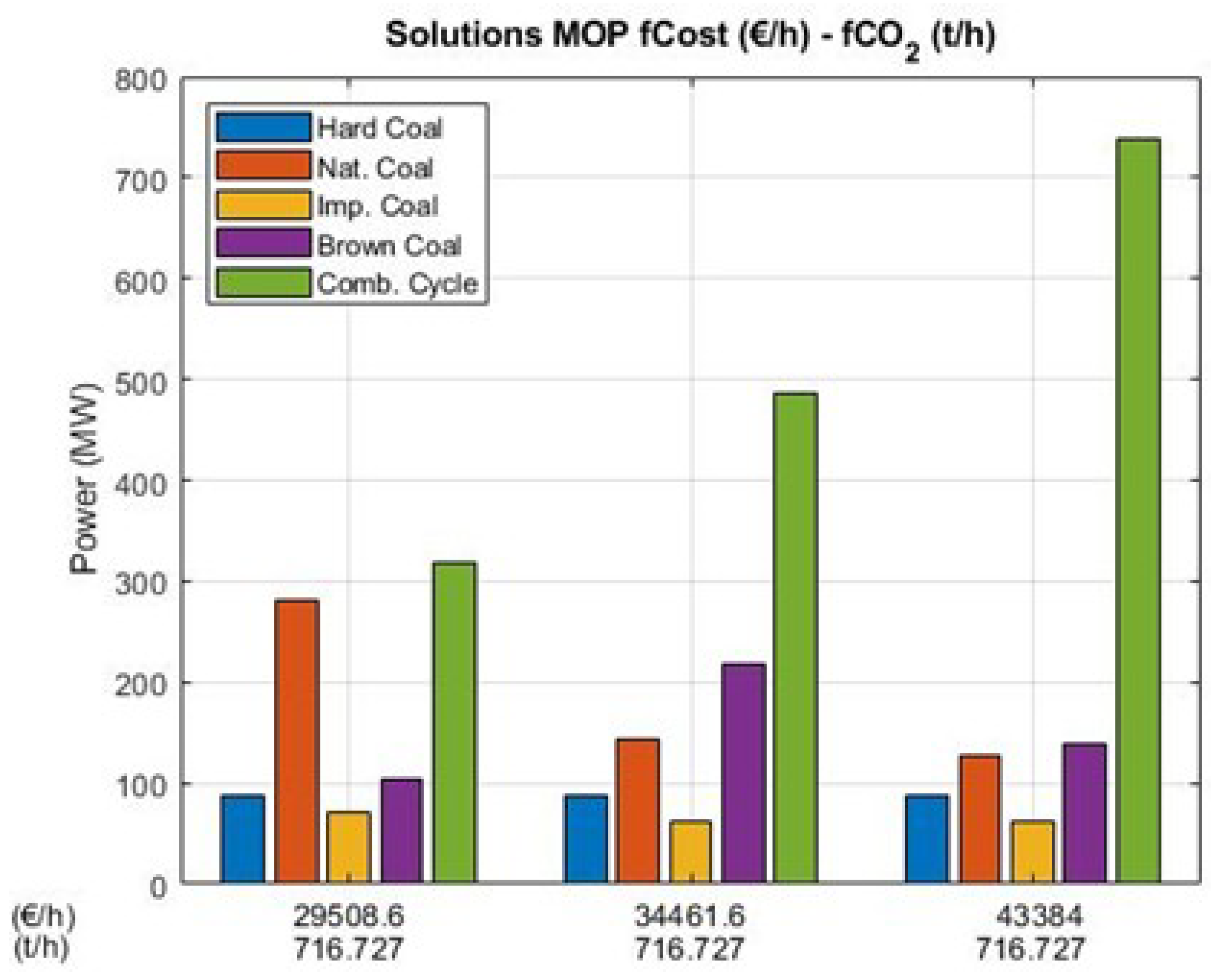
Figure 21.
: Optimal costs variations vs wind power deviations respecting the 50 % emissions range.
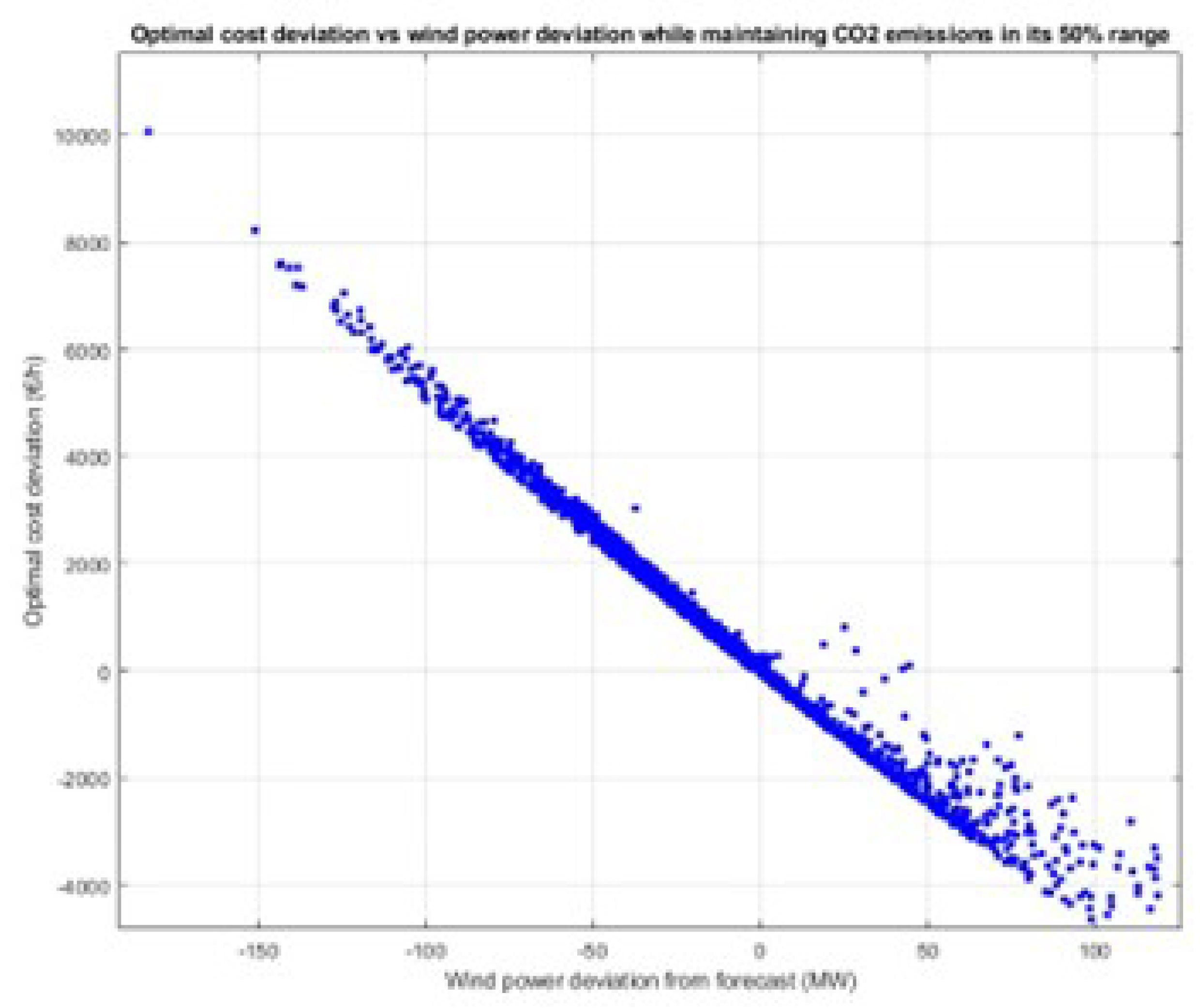
Figure 22.
: Histogram of Cost Simulation Results.
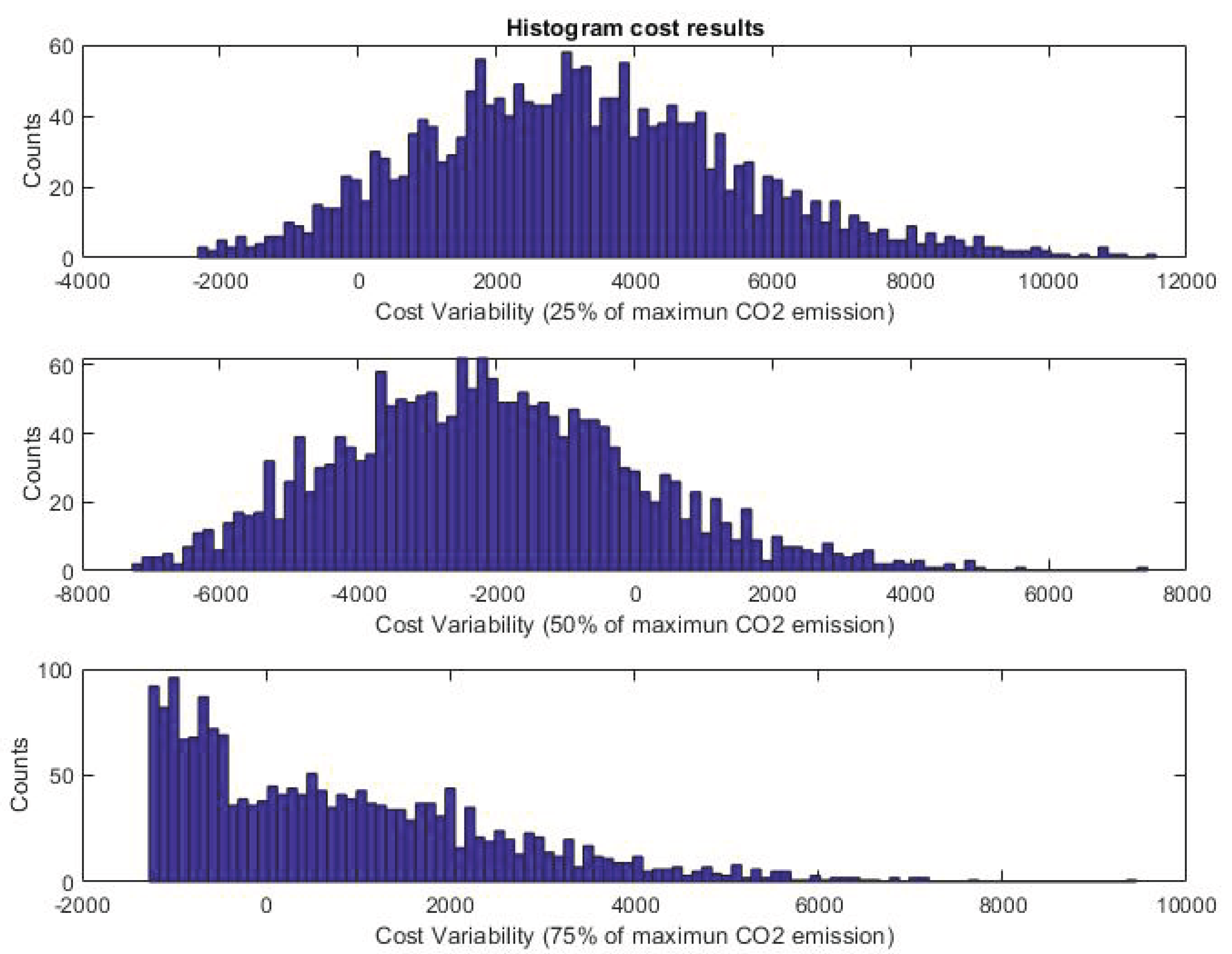

Table 1.
Characteristics Of The Fuels And The Power Plants Used.
| Power Plant | C(%) | S(%) | LHV (kJ/kg) | Cost (€/MWh) | (MW) |
|---|---|---|---|---|---|
| Hard Coal | 60 | 1.3 | 22,000 | 8 | 350 |
| National Coal | 60 | 1.3 | 22,400 | 8 | 225 |
| Imported Coal | 70 | 0.6 | 26,350 | 8 | 250 |
| Brown Coal | 33 | 4.5 | 14,650 | 4.673 | 350 |
| Combined Cycle / Natural Gas | 74.2 | 0 | 50,006.5 | 26 | 400 |
Table 2.
General Prediction Errors Data Summary.
| Program Deviation | Nominal Power | Prediction errors mean Value | Statistical deviation of the prediction errors |
|---|---|---|---|
| Windfarm A | 13 MW | -0.277 MW | 2.77 MW (19 %) |
| Windfarm B | 46.6 MW | 0.92 MW | 7.67 MW (16.5 %) |
Table 3.
Estimation of Kernel Distribution Models.
| Max Power | Bid | Kernel | Bandwidth |
|---|---|---|---|
| 30.94 MW | 16.66 MW | Normal | 2.40774 |
| 30.94 MW | 28.56 MW | Normal | 1.02929 |
| 61.1 MW | 32.9 MW | Normal | 4.75477 |
| 61.1 MW | 56.4 MW | Normal | 2.03264 |
| 218.55 MW | 70.5 MW | Normal | 8.80877 |
| 110.67 MW | 71.4 MW | Normal | 6.00953 |
Table 4.
Summary of Simulation Results.
| Emissions [pu] | Emissions [] | Pareto Cost Solution [k€/h] | Mean Real Cost [k€/h] | Standard Deviation [k€/h] |
|---|---|---|---|---|
| 0.25 | 716.7 | 34.36 | 35.07 | 2.324 |
| 0.5 | 792.8 | 31.83 | 32.36 | 2.195 |
| 0.75 | 867.0 | 29.61 | 30.43 | 1.718 |
Disclaimer/Publisher’s Note: The statements, opinions and data contained in all publications are solely those of the individual author(s) and contributor(s) and not of MDPI and/or the editor(s). MDPI and/or the editor(s) disclaim responsibility for any injury to people or property resulting from any ideas, methods, instructions or products referred to in the content. |
© 2025 by the authors. Licensee MDPI, Basel, Switzerland. This article is an open access article distributed under the terms and conditions of the Creative Commons Attribution (CC BY) license (https://creativecommons.org/licenses/by/4.0/).
Copyright: This open access article is published under a Creative Commons CC BY 4.0 license, which permit the free download, distribution, and reuse, provided that the author and preprint are cited in any reuse.


