Submitted:
07 November 2025
Posted:
10 November 2025
Read the latest preprint version here
Abstract
Designing hyperelastic porous microstructures under finite strain is challenging because bending, buckling, contact, and densification interact to produce nonconvex and one-to-many relations between topology and response. We present HyperDiff, a conditional diffusion framework that reformulates inverse design as probabilistic sampling rather than deterministic regression. A compact B-spline encoding of the target force--displacement curve captures the system’s energy-evolution trend, providing temporal and mechanical context that guides the denoising process toward physically consistent and stage-correct configurations. The workflow integrates GRF-based topology generation, constitutive calibration, large-deformation finite-element simulations, and quasi-static compression experiments. Across held-out and interpolated targets, the generated microstructures accurately reproduce sequential deformation stages (bending → buckling → densification) and global responses, with deviations typically below 10\%, while preserving manufacturability and one-to-many design diversity. The current implementation focuses on two-dimensional unit cells under quasi-static compression, yet the framework is extensible to 3D, multi-resolution, and multi-physics systems. By combining physics-aware conditioning with generative sampling, HyperDiff establishes a practical front end for mechanics-based design workflows, applicable to programmable soft actuators, impact-energy absorbers with tunable plateaus, and rapid exploration of nonlinear architected materials for soft and deformable systems.
Keywords:
hyperelastic microstructures
; inverse design
; conditional diffusion models
; large deformation
; generative modeling
1. Introduction
Mechanical metamaterials are architected solids whose effective properties are governed primarily by geometry rather than base material composition. These engineered structures enable functionalities such as lightweight energy absorption, programmable deformation, multistability, and shape morphing, with applications in aerospace structures, biomedical devices, soft robotics, and protective systems [1,2,3,4,5,6,7]. Recent work has shown that controlled buckling, snap-through, and phase-transition-like transformations can be used to realize tunable force–displacement or stress–strain responses on demand, rather than relying on the intrinsic response of a homogeneous material [8,9]. As a result, the design of metamaterials is increasingly viewed not only as structural layout design, but as direct control over nonlinear mechanical behavior for specific functions [10,11,12,13].
Although many classes of high-performance metamaterials have been demonstrated, their design remains challenging. Conventional “forward” workflows typically begin with a candidate topology inspired by natural templates such as cellular, porous, or origami-like patterns, and then iterate through simulation and manual refinement [8,14,15]. This approach has produced notable successes, including ultralight lattices and multistable snapping systems, but it is time-consuming, problem-specific, and scales poorly when the goal is to match a prescribed mechanical response under large deformation [5,7]. In modern applications, designers increasingly require materials whose global response is staged or switchable — for example, an initially compliant regime for impact mitigation, followed by a stiffening or locking regime for load-bearing [4,6,9]. Achieving such behavior by manual tuning is difficult because performance, manufacturability, and stability must be balanced simultaneously [10,12,16].
Inverse design aims to address this challenge by reversing the traditional workflow: instead of starting from geometry and predicting behavior, it starts from the desired mechanical response and searches for a compatible microstructure [17,18,19]. This paradigm is particularly attractive for metamaterials, where the mapping from geometry to response is often nonlinear, history-dependent, and governed by local instabilities such as buckling and self-contact [20]. With recent advances in machine learning, inverse design is increasingly seen as a path toward performance-by-design structures in both structural and functional materials [10,11,12,13,21].
Current machine-learning-based inverse design strategies can be broadly grouped into two categories. The first category is parametric or low-dimensional design. In these approaches, the metamaterial is represented using a finite set of geometric parameters, and surrogate models or neural networks are trained to map those parameters to mechanical performance [22,23,24,25]. These models can then be coupled with heuristic or evolutionary optimizers to efficiently explore the parameter space and produce customized load–displacement curves for specific structure families [22,26]. Although computationally efficient and interpretable, such methods are constrained by the assumed parameterization. They typically operate within a predefined family of unit cells (e.g., shells, graded lattices, or spinodoid structures), and may struggle to capture drastic topological changes or complex post-buckling behavior [24,25,26].
The second category is non-parametric generative design, in which the microstructure is treated directly as an image-, voxel-, or implicit-surface field rather than a hand-crafted geometric template [27,28,29,30]. This class of methods leverages deep generative models to learn high-dimensional structure–property relationships from data. Convolutional neural networks and generative adversarial networks (GANs) have been used to synthesize topologies with target stiffness or target bulk modulus, and to encode the geometry of cellular materials in an implicit representation [27,28,31,32]. Variational autoencoders (VAEs) take a related approach by embedding complex microstructures into a smooth latent space, which can then be searched or optimized for target properties [26,33,34].
More recently, diffusion models have emerged as a powerful alternative for generative inverse design. These models iteratively transform random noise into structured outputs by learning a reverse denoising process [35,36,37,38]. Unlike GANs, diffusion models are known for their sampling stability and controllability. They have been applied to reconstruct complex microstructures, generate energy-absorbing metamaterials tailored to specified loading curves, and model time-dependent deformation fields in nonlinear metamaterials under load [39,40,41,42,43,44]. These advances suggest that generative modeling can move beyond “shape suggestion” and toward direct synthesis of structures with prescribed mechanical behavior.
However, important challenges remain for the inverse design of hyperelastic metamaterials that undergo large strain, geometric nonlinearity, and path-dependent softening. Under compression, such microstructures often exhibit multiple sequential regimes: an initially compliant phase dominated by bending, followed by buckling and stress softening, and eventually densification accompanied by contact and rapid stiffening [9,20,45,46]. Capturing these regimes is essential for applications such as impact mitigation and reusable energy absorption. At the same time, it is difficult for standard optimization-based approaches because the mapping from topology to force–displacement behavior is strongly nonconvex and not easily parameterized [22,24,26]. While recent diffusion-based studies have demonstrated controllable generation for elastoplastic or energy-absorbing systems [39,40,44], there is still limited work on learning a direct mapping from a target nonlinear force–displacement curve to a manufacturable hyperelastic porous topology that remains physically realistic under large deformation, including buckling and post-buckling contact.
A key difficulty in this field lies in the intrinsic ill-posedness of the inverse mapping between geometry and mechanical response. For hyperelastic porous microstructures, the mapping from a target force–displacement curve to geometry is inherently ill-posed for four coupled reasons: (i) non-uniqueness—distinct topologies can realize nearly identical curves, while similar patterns may diverge; (ii) nonconvexity and mode switching introduced by buckling, contact, and densification; (iii) high sensitivity of the response to small geometric perturbations (e.g., manufacturing tolerances); and (iv) the limited descriptive power of low-dimensional features such as volume fraction. These challenges motivate the adoption of a probabilistic, condition-guided generative formulation that can naturally represent one-to-many mappings instead of enforcing a single deterministic inverse. Representative examples illustrating these phenomena are provided in Section 3.
To address this gap, we propose HyperDiff, a conditional diffusion-based inverse design framework for hyperelastic porous microstructures with nonlinear mechanical responses, as outlined in Figure 1. The core idea is to treat the desired global response — here expressed as a force–displacement curve — as a conditioning signal for a denoising diffusion probabilistic model (DDPM) [35,36]. The diffusion model is implemented using a U-Net backbone with residual connections and attention-based conditioning [28,37,39,47,48], which enables it to generate candidate microstructure topologies directly in image form. To supply meaningful training data, we construct an integrated pipeline that (i) procedurally generates porous microstructures, (ii) calibrates a hyperelastic constitutive model for the base material using tensile experiments, (iii) simulates large-deformation compression via finite element analysis to obtain full force–displacement curves, and (iv) encodes those curves in a compact form suitable for conditional generation [10,16,45,46,49]. The resulting framework links data generation, inverse design, forward simulation, and experimental validation.
In summary, this work demonstrates that conditional diffusion modeling can be used to generate diverse and physically consistent microstructures that reproduce prescribed nonlinear force–displacement behavior, including regimes dominated by bending, buckling, softening, and densification. By focusing on hyperelastic, large-strain responses — a setting where topology, instability, and contact play central roles — this study aims to contribute to the practical integration of generative AI tools into the design workflow of nonlinear architected materials [9,12,13,21,44].
The remainder of this article is organized as follows. Section 2 presents the theoretical basis of denoising diffusion probabilistic models and details the proposed HyperDiff framework. Section 3 describes the dataset generation pipeline, including GRF-based topology synthesis, material characterization, and finite element (FE) simulation of force–displacement responses. Section 4 explains the model training strategy, including conditioning, data normalization, and key hyperparameters. Section 5 reports numerical results on both test and interpolated targets to assess performance and generalization. Section 6 presents experimental verification via quasi-static compression tests and compares measurements with simulations. Finally, Section 8 summarizes the main findings, discusses limitations, and outlines future directions.
2. Methodology
This section details the theoretical framework of HyperDiff. Section 2.1 outlines the principles of the denoising diffusion probabilistic model (DDPM), while Section 2.2 describes the custom neural network architecture developed for this research.
2.1. Generative Diffusion Model Theory
DDPMs comprise two processes: a forward process that incrementally adds noise to the data, and a reverse process that learns to denoise. The reverse process starts with pure Gaussian noise and iteratively refines it into a coherent data sample over a sequence of steps. At each step, a neural network acts as a denoiser, predicting and removing a small amount of noise to gradually recover the underlying data structure. Therefore, the reverse process can be understood as a sequence of denoising operations that collectively reconstruct data from pure noise.
2.1.1. Forward Process
The purpose of the forward process is to systematically and controllably corrupt an initial data sample (e.g., a clear microstructure image) into pure, unstructured noise. This is achieved through a fixed Markov chain, where each state depends only on the preceding state , analogous to a time-stepping scheme in a physical simulation. This gradual corruption process can be conceptually related to stochastic relaxation in physical systems, where disorder increases step by step in the forward direction and order is progressively restored during the reverse diffusion. This process unfolds over T discrete time steps, generating a sequence of increasingly noisy latent variables .
At each time index t, the preceding sample is perturbed by a small Gaussian increment. The core of this operation is described by the conditional probability:
where is a small, positive constant defined by a variance schedule, with . This schedule controls the magnitude of noise added at each step. The term acts as a scaling factor that slightly shrinks the previous state , while the variance defines the newly added noise.
A key property of this formulation, which makes it computationally tractable, is that we can sample at any arbitrary time step t directly from the initial data , without having to iterate through all intermediate steps. This closed-form solution is obtained by defining and , which yields:
This equation can be understood as a weighted sum. The terms and represent the scaling factors for the original signal () and the noise (), respectively. As t increases, decreases towards zero, causing the contribution from the original data to diminish while the contribution from the noise grows.
This process ensures that as t approaches the final time step T, the cumulative product becomes nearly zero. Consequently, the state loses all information about the original sample and converges to an isotropic Gaussian distribution, . This provides a well-defined starting point of pure noise from which the reverse process can begin reconstruction.
2.1.2. Reverse Process
The generative mechanism of the model is driven by the reverse process. Its goal is to reverse the noising procedure by starting with pure Gaussian noise and iteratively denoising it, step by step, to recover a sample from the original data distribution . This is modeled as a learned Markov chain parameterized by a neural network :
where the neural network learns both the mean and the scalar variance . However, Ho et al. [35] found that fixing the variance to a set of predefined constants and only learning the mean resulted in more stable training and higher-quality samples. Following this standard practice, we set to a non-learned hyperparameter (typically or ).1 The network’s task is therefore reduced to learning only the mean .
The primary challenge is that the true reverse conditional probability is intractable. Calculating it would require marginalizing over the entire (unknown) data distribution, which is computationally infeasible. However, a crucial insight is that if we also condition this probability on the initial data sample , the posterior becomes tractable and follows a Gaussian (normal) probability distribution:
where the mean and variance are known functions of the forward process variables (). While is unknown during inference, this tractable posterior is invaluable during training, as it provides a target for the neural network.
To make this insight practical for training, we use a reparameterization trick. Recall from the forward process (Equation (2)) that any noisy sample can be expressed in terms of the initial sample and the noise that was added. By rearranging that equation, we can express as:
Substituting this expression for into the equation for the tractable posterior mean (Equation (4)) allows us to express that mean as a function of the observable state and the noise :
This reformulation reveals a critical simplification: learning the complex posterior mean is equivalent to learning the noise vector that was added at step t. Predicting this noise is a more direct and stable objective for a neural network.
Therefore, instead of training the network to predict directly, we train a network to predict the noise component from the noisy sample at time step t. The learning objective reduces to minimizing the mean squared error between the ground-truth noise and the predicted noise, a widely adopted and effective loss:
where denotes the expectation over the distribution of data, time steps, and noise, which in practice is approximated by randomly sampling these components at each step of training. Accordingly, all experiments reported below optimize the L2 (mean-squared) loss in Equation (7), and the hyperparameter summary reflects the same objective.
2.1.3. Conditional Generation with Classifier-Free Guidance
To guide the generation process with auxiliary information , such as force–displacement data, we employ the classifier-free guidance (CFG) strategy [36]. This technique allows a single model to learn both conditional and unconditional generation pathways, enabling robust control over the output at inference time.
The core idea is to modify the training process. With a fixed probability (e.g., 10–20% of the time), the conditioning vector is replaced with a learned null token, ∅. This forces the network to learn to predict the noise both with and without conditioning information. The training objective is therefore to predict the noise from the noisy state , conditioned on either the true label or the null token ∅:
where is randomly replaced by ∅ for a subset of the training batch.
The true power of CFG is realized during inference. At each denoising step t, the model makes two predictions for the noise: one conditional, , and one unconditional, . These are combined to form a guided prediction :
where w is the guidance scale, a hyperparameter that controls the strength of the conditioning. When , generation is purely unconditional. When , the model is pushed to generate samples that more strongly adhere to the condition . This guided noise estimate is then used in the reverse process equations (e.g., Equation (6)) to compute the mean of the denoised sample .
2.2. HyperDiff Architecture
To achieve the inverse design objectives of the HyperDiff framework, the neural network must predict the noise term at each reverse diffusion step, conditioned on the target force–displacement curve . This requires the model to extract features across multiple spatial scales while coupling local geometric patterns with global mechanical constraints. A U-Net backbone, with its symmetric encoder–decoder structure and skip connections, provides a suitable foundation for this purpose.
The proposed architecture builds upon the conventional diffusion-model U-Net [35,50] and introduces two key modules that enhance its representational and physical consistency: residual blocks and spatial transformers. As illustrated in Figure 2, panel (a) depicts the overall denoising process with a multi-scale U-Net backbone, which progressively refines the noisy microstructure representation . The encoder extracts hierarchical features from fine to coarse scales, while the decoder reconstructs the topology by combining deep semantic and shallow geometric information through skip connections.
Panel (b) shows the residual block structure. Each residual block acts as a local adaptive filter that stabilizes gradient flow and captures deformation-sensitive features. The diffusion time-step embedding is injected into the block using FiLM-style modulation, allowing the network to dynamically adjust its denoising behavior according to the current diffusion state.
Panel (c) presents the spatial transformer module, which captures long-range correlations and integrates the conditioning mechanical information. Through self-attention, the model learns global spatial dependencies within the feature map, while cross-attention propagates the target force–displacement condition across the entire field, ensuring that every spatial region adheres to the prescribed macroscopic mechanical behavior.
By jointly employing residual blocks for localized learning and spatial transformers for global constraint propagation, HyperDiff achieves a balanced local–global coupling mechanism. This design ensures that the generated microstructures are both topologically coherent and mechanically consistent with the desired target responses.
3. Dataset Generation
A comprehensive dataset mapping microstructural topologies to their nonlinear mechanical responses is essential for training the HyperDiff model. This section details the three-stage pipeline developed to generate this dataset: (1) procedural generation of diverse microstructure topologies using a Gaussian random field (GRF) method, (2) experimental characterization of the hyperelastic material properties, and (3) large-scale finite element simulation to compute the force–displacement response for each topology.
3.1. Microstructure Topology Generation
To build a physically grounded dataset of porous microstructures with diverse geometric and mechanical characteristics, a two-dimensional Gaussian random field (GRF) sampling approach is employed, as illustrated in Figure 3(a). A continuous GRF is first generated over a square domain and then thresholded to obtain a binary solid–void distribution. To ensure structural integrity and manufacturability, connectivity and coverage thresholds are applied, and a four-side symmetric topology is reconstructed by mirroring the binary pattern. Contour detection, sampling, and smoothing operations are subsequently performed to remove irregularities and obtain well-defined smooth boundaries suitable for finite element analysis. This process produces geometrically diverse yet physically consistent unit cells that serve as the input domain of the HyperDiff framework. The corresponding material calibration and finite element simulation procedures, shown in Figure 3(b,c), provide the ground-truth mechanical responses used to supervise the conditional diffusion model.
The GRF is generated in the frequency domain to control its spatial characteristics via a prescribed power spectrum. First, a complex-valued field is constructed from independent standard normal variables and for each wave vector :
A power spectrum filter is then applied to shape the field’s correlations:
where the parameter controls the spatial correlation of the field, and is a small constant to prevent singularities. The real-space representation is obtained via the inverse Fourier transform:
To ensure remains strictly real before thresholding, we enforce Hermitian symmetry by constructing (with consistent random phases) prior to the inverse FFT, so the recovered field is physically meaningful for subsequent binarization.
After normalization and Gaussian smoothing, the field is binarized using a threshold t to define the material phase :
Finally, to form a fully symmetric structure, the base microstructure quadrant is mirrored across both axes:
where denotes the spatial coordinates and N is the grid size. This GRF-based method efficiently generates a diverse set of porous microstructures with rich, multiscale features suitable for training a robust generative model.
3.2. Material Characterization and Hyperelastic Model Calibration
To characterize the nonlinear mechanical behavior of the base material used in the generated microstructures, uniaxial tensile tests were conducted on thermoplastic polyurethane (TPU) specimens in accordance with the GB/T 228.1–2021 standard. The experimental setup, specimen geometry, and resulting stress–strain curves are shown in Figure 3(b). The tests were performed using a TFW-100S universal testing machine at a constant displacement rate of , corresponding to a nominal strain rate of , which satisfies the quasi-static loading condition. Both engineering and true stress–strain curves were recorded, and the data were fitted using a second-order Ogden hyperelastic model to capture the material’s large-deformation behavior. The fitted curve shows excellent agreement with the experimental data, confirming that the Ogden model can accurately describe the nonlinear, strain-hardening response of TPU. The calibrated parameters were subsequently applied to all finite element simulations in Figure 3(c), ensuring consistency between the experimental characterization and numerical modeling stages of the dataset.
Assuming material incompressibility, the engineering data were converted to true stress () and logarithmic strain ():
where F is the applied load, is the initial cross-sectional area, and is the engineering strain. To enable finite element simulations, the true stress–strain data were fitted using the Ogden hyperelastic model [49], which provided the best fit. Its strain energy density function is expressed as:
where are the deviatoric principal stretches, and , , and are material parameters. The Ogden model is particularly suitable for capturing the nonlinear stiffening behavior of hyperelastic materials. The fitted parameters obtained from Abaqus are listed in Table 1. When a reported parameter satisfies (as for the first term in Table 1), the implementation evaluates the limit, which is equivalent to inserting a neo-Hookean term with modulus and avoids the apparent singularity in the prefactor.
3.3. Finite Element Simulation and Force–Displacement Responses
To evaluate the mechanical responses of the generated microstructures and establish the ground-truth data for model training, finite element simulations were performed on each unit cell using the calibrated hyperelastic parameters obtained from Figure 3(b). In metamaterial design, full assemblies typically require 5–10 repeating unit cells to achieve homogenization, which considerably increases computational cost. To balance efficiency and fidelity, the simulations in this study focused on individual unit cells, which sufficiently capture the intrinsic nonlinear mechanisms relevant to the inverse-design task.
As illustrated in Figure 3(c), each microstructure was placed between two rigid plates and subjected to uniaxial compression under quasi-static loading conditions, and the corresponding von Mises stress contours were used to visualize the evolution of local stress concentrations during deformation. The simulations were conducted in a two-dimensional plane-stress setting with appropriate symmetry and boundary constraints to represent periodic behavior. The computed force–displacement curves exhibit the characteristic three-stage compressive response of porous hyperelastic materials: (i) an initial elastic regime dominated by frame bending and stretching, (ii) a nonlinear instability regime associated with progressive buckling and softening, and (iii) a final densification regime where pore collapse leads to a rapid increase in stiffness. These stages correspond closely to the deformation and stress-localization mechanisms observed in quasi-static compression experiments, ensuring that the dataset remains both physically interpretable and experimentally consistent.
All simulations were performed in Abaqus/Explicit using the Ogden hyperelastic model with parameters listed in Table 1. The upper rigid plate was coupled to a reference point for displacement control, while the lower plate was fully constrained. Contact definitions included hard contact with a tangential friction coefficient of 0.18 between the plates and the microstructure, as well as general contact for internal self-interaction to prevent element interpenetration during large deformation. The microstructure was meshed with CPS3 (plane-stress) triangular elements (seed size 2.5 mm), and the rigid plates were meshed with R2D2 elements (seed size 5.0 mm). A smooth-step amplitude curve was used to impose 60% compressive strain quasi-statically. The explicit central-difference integration scheme was adopted for its robustness in handling large deformations and complex contact evolution without convergence issues.
A fully automated workflow was implemented through a Python script based on the Abaqus API. The script automatically performs geometry construction, Boolean operations, contact definition, material assignment, mesh generation, and batch job submission, enabling efficient multi-core parallel simulations of approximately 20,000 unique microstructures. This large-scale dataset captures not only the canonical three-stage responses but also non-classical two- or four-stage behaviors caused by local instabilities and complex topological patterns. Notably, microstructures with similar volume fractions can exhibit markedly different force–displacement responses, while distinct topologies may produce nearly identical curves. This non-unique structure–property mapping is visualized in Figure 4 and Figure 5, which highlight the diversity, nonconvexity, and weak identifiability of the dataset—factors that make the inverse problem intrinsically challenging and motivate the adoption of data-driven generative frameworks such as HyperDiff.
4. Model Training Strategy
The primary objective of our training strategy is to establish a reliable mapping from a target force–displacement curve to a corresponding microstructural design. A common approach in related literature, such as that by [39], involves conditioning a model on simplified mechanical responses like stress–strain curves. However, such a setup can be ineffective for designing microstructures that exhibit complex behaviors such as structural instability and buckling. The limitation lies in the indirect nature of this mapping, where the model learns from static geometry without sufficient information about the dynamic mechanical response.
To provide a compact and robust conditioning signal for the diffusion model, the force–displacement curves are (i) smoothed and de-noised, then (ii) parameterized by B-spline.
B-Spline Representation.
Here are control-point coefficients and are k-th order basis functions defined by a nondecreasing knot vector .
Min–Max Normalization.
Feature Vector Construction.
The final 1D feature vector concatenates normalized coefficients and knots (ascending order within each group):
This compact vector preserves the essential curve shape while improving training efficiency, numerical stability, and generalization.
Hyperparameters
The key hyperparameter settings employed in our training process are detailed in Table 2. This configuration was optimized to balance model capacity, training stability, and computational efficiency.
This training strategy provides a stable conditioning signal for the diffusion model, supporting accurate and interpretable inverse design predictions under complex deformation mechanisms such as buckling and densification.
5. Results and Validation
We evaluated HyperDiff’s performance through systematic numerical experiments. We selected four reference force–displacement curves from the test set as targets. For each target, we generated 50 microstructures by sampling different random noise vectors, thereby assessing the model’s ability to produce diverse yet mechanically consistent designs.
All generated microstructures were analyzed using the same Abaqus finite element setup described in Section 3.3. To quantify performance, we used the normalized root-mean-square error (NRMSE), , between the generated force response F and the target response :
where provides a single, curve-wide normalization factor that is strictly positive even when the target force crosses or equals zero. This definition keeps the metric scale-invariant without incurring divisions by at the unloaded state, so the entire curve—including the initial flat segment—contributes smoothly to the reported error. Consequently, a 10% deviation on a low-force (soft) curve is weighted just as heavily as a 10% deviation on a high-force (stiff) curve, ensuring the model is evaluated fairly across a diverse range of mechanical responses.
5.1. Performance on Test Curves
To assess HyperDiff’s generalization to unseen data, we selected four representative force–displacement curves from the test set, covering both weakly and strongly nonlinear behaviors. Figure 6 (left block) summarizes the results: the top row reports per-case profiles of the normalized pointwise relative error along the displacement axis, the middle row shows NRMSE distributions over 50 stochastic generations, and the bottom row presents a representative force–displacement overlay for Case 1. For three of the four cases, the median error was below 7%, and Case 4 achieved a median error of approximately 0.4%. Additional per-target overlays and the corresponding topologies for the remaining test cases are provided in Figure 7, which further illustrate consistent shape matching and one-to-many topology diversity.
As shown in Figure 6, the generated microstructures and their corresponding force–displacement curves for the minimum- and median-error samples closely match their targets. Notably, the generated microstructures exhibit significant topological diversity while achieving nearly identical mechanical performance. For example, the best- and median-performing structures for Case 1 share a similar overall layout but differ in their internal connectivity. This one-to-many mapping capability is a key advantage of our generative approach, providing designers with a range of valid solutions for a single performance target.
5.2. Performance on Interpolated Curves
To further test HyperDiff’s generalization, we evaluated its ability to generate microstructures for interpolated force–displacement curves—targets that lie between samples in the training data distribution. We created four sets of interpolated targets by linearly combining pairs of curves from the training set (see Figure 6, right block).
The results indicate that HyperDiff exhibits strong interpolation capability. As shown in Figure 6, the median error was below 8% in three of the four interpolation cases, while Interp. 4 achieved a notably low median error of approximately 0.4%. In contrast, Interp. 2 showed a higher median error (around 16%), which can be attributed to its pronounced nonlinear characteristics, making it a more challenging target for accurate design.
The generated microstructures in Figure 6 successfully match the interpolated mechanical targets, with minimum errors below 6% in all cases. Again, the model produces topologically diverse solutions for each target. For instance, the minimal-error and median-error structures for Interp. 3 both feature a primary “X”-shaped load path but differ in their central region. This confirms HyperDiff’s ability to generalize beyond the training set and explore the design space to find novel and effective microstructures. Complementary per-target overlays and the corresponding topologies for the remaining interpolated cases are presented in Figure 7.
6. Experimental Verification
To validate the predictive accuracy and physical consistency of the proposed HyperDiff framework, a series of quasi-static compression experiments were performed on representative energy-absorbing metamaterial specimens. The samples were fabricated via 3D printing (additive manufacturing) and tested using a universal testing machine under a constant compression rate of 2 mm/min, ensuring quasi-static loading conditions. During the tests, force and displacement data were synchronously recorded to accurately capture the mechanical responses. The experimental setup enabled continuous observation of deformation patterns and ensured repeatability of the results. A comprehensive comparison between experimental and simulation results is presented in Figure 8.
As shown in Figure 8, the left column presents the force–displacement curves obtained from the target, numerical simulation, and experimental measurements (black dashed, red dotted, and blue dash–dot lines, respectively). The normalized root-mean-square error (NRMSE) was used to evaluate prediction accuracy. For the representative case shown, the NRMSE between the experimental and target curves was 9.41%, between the simulated and target curves 6.10%, and between the experimental and simulated curves 4.42%. These results confirm that the HyperDiff model can accurately reproduce the nonlinear mechanical behavior of the designed metamaterials.
The right-hand side of Figure 8 illustrates the deformation sequences (stages I–VI) under progressive compression. The top row shows the simulated von Mises stress contours, while the bottom row presents the corresponding experimental deformation images. As strain increased, small internal pores closed first (stages II–III). When the displacement reached approximately 15 mm (stage IV), the central pore was nearly closed. Further loading caused contact between the upper and lower beams and the compression plate, leading to a rapid increase in tangent stiffness. The regions of high stress in the simulations correspond closely to the zones of visible large-strain localization and contact-induced densification in the experiments, indicating that the model captures the essential physical mechanisms rather than merely fitting data correlations. This agreement reinforces the interpretability and physical reliability of the proposed framework.
A detailed analysis of the first case in Figure 8 is presented as a representative example. The other tested specimens exhibited consistent deformation modes and response trends, demonstrating the robustness of both the model and experimental validation process.
7. Discussion
The results in Section 5 and Section 6 show that HyperDiff can recover the main features of nonlinear force–displacement responses for hyperelastic porous microstructures across both numerical simulations and experiments. This section provides a mechanics-aware interpretation of these results, explains how the conditional diffusion process organizes structure–response relations, and outlines the scope and limitations of the present framework.
7.1. From a Difficult Inverse Problem to a Tractable Generative View
Inverse design in the large-deformation hyperelastic regime is challenging because the macroscopic response arises from multiple sequential mechanisms—early-stage bending compliance, instability-induced softening, contact-mediated load transfer, and late-stage densification. These mechanisms lead to a highly nonconvex, inherently one-to-many mapping between topology and response. Small geometric perturbations can trigger a completely different instability path, while distinct microstructures may yield similar global responses. Under such conditions, parametric regression or gradient-based optimization often becomes trapped in local minima and lacks generality across design families.
The present framework addresses this difficulty by shifting from “solve-for-the-one” to “sample-from-the-set.” Instead of pursuing a deterministic inverse map, HyperDiff learns the conditional distribution of admissible topologies given a target response. This generative perspective is consistent with the physical nature of the problem: for a prescribed force–displacement curve, multiple feasible microstructures usually exist. Sampling diverse candidates and retaining those verified by forward analysis thus provides a pragmatic and robust solution.
7.2. A Mechanics-Aware Reading of the Diffusion Process
Although diffusion models are typically introduced as statistical denoisers, the present results suggest a mechanics-aware interpretation in this context. The U-Net backbone with residual connections captures local void morphologies, while spatial transformers ensure global coherence consistent with compression load paths. During denoising, structural features emerge in a physically ordered sequence: early iterations determine initial compliance (void slenderness and ligament curvature), mid-stage updates control buckling onset and amplitude, and later iterations form load-bearing bridges that sustain densification.
Hence, the iterative sampling process does not merely “reconstruct an image,” but instead relaxes toward configurations that are both statistically plausible and mechanically admissible under the given conditioning signal. This explains why the generated microstructures reproduce not only the overall force–displacement trends but also the observed deformation stages in both simulation and experiment.
7.3. Conditioning Via Force–Displacement Curves as Energy-Trend Guidance
A distinctive element of HyperDiff lies in its conditioning strategy based on a compact B-spline representation of the target force–displacement curve. Although no explicit energy integration is enforced, the curve inherently reflects the cumulative exchange of mechanical work during loading; the corresponding B-spline coefficients thus serve as a concise descriptor of the system’s energy-evolution trend. Conditioning on this vector provides temporal (stage-wise) and mechanical (stiffness/softening/densification) context to the generator. Empirically, this guidance enables the model to converge toward structures that exhibit the correct sequence of deformation mechanisms, not merely the right scalar magnitudes.
This interpretation also clarifies the difference from encodings that treat the curve as a generic signal: here, the conditioning is designed to carry physically meaningful information. Extending the conditioning vector with explicit cumulative-energy or stage-indicator terms is straightforward if finer phase control is desired in future studies.
7.4. Applicability, Robustness, and Boundaries
The current implementation focuses on two-dimensional unit cells at a fixed image resolution and on quasi-static compression of a calibrated hyperelastic material. Within this scope, the method is robust: it achieves low deviations on held-out targets, maintains accuracy on interpolated curves, and yields printed samples whose deformation patterns match simulations. These results support that the learned topology–response relationships are physically meaningful rather than numerical coincidences.
At the same time, clear boundaries exist. Out-of-plane effects are excluded by design; rate dependence, viscoelasticity, and thermal coupling are not considered; and the minimum printable feature size is constrained by the image resolution. Diffusion-based sampling is computationally more demanding than direct regression, but the gain in solution diversity is valuable in nonconvex design spaces. These factors should be kept in mind when generalizing beyond the current dataset.
7.5. Relation to Prior Inverse Design Studies
Compared with inverse design frameworks developed for elastoplastic or energy-absorbing systems, the present study targets the finite-strain hyperelastic regime, where geometric and constitutive nonlinearities interact. Methodologically, the main differences are: (i) a generative, distributional formulation of the inverse problem; (ii) a physically meaningful conditioning vector encoding the energy-evolution trend; and (iii) validation of both global responses and stage-wise deformation modes through numerical and experimental means. These aspects explain the consistent performance observed for highly nonlinear targets that typically challenge deterministic regressors.
7.6. Practical Implications
In practice, HyperDiff can be used in two complementary modes. First, as a design exploration tool, it rapidly proposes multiple distinct microstructures for a single target, allowing post-selection under additional criteria such as manufacturability or stress localization. Second, as a front-end generator, it provides physically consistent initial designs for subsequent physics-based optimization. Both usages exploit the model’s diversity while maintaining mechanical consistency.
Summary. When conditioned on an energy-trend encoding of the desired response, the diffusion model acts as a probabilistic sampler over physically feasible topologies in a nonconvex design space. This perspective reconciles data-driven generation with mechanics-based understanding and explains the cross-consistency observed between simulations and experiments.
8. Conclusions and Future Work
This work introduced HyperDiff, a conditional diffusion framework for the inverse design of hyperelastic porous microstructures undergoing large deformation, buckling, softening, and densification. By modeling the distribution of admissible topologies conditioned on a physically meaningful encoding of the target force–displacement path, the framework bridges response specification, generative synthesis, and physical validation.
Main Contributions.
- Generative formulation of a nonconvex inverse problem. The inverse design problem is reformulated as conditional sampling rather than deterministic inversion, enabling one-to-many solutions consistent with the inherent non-uniqueness of the finite-strain hyperelastic regime. This improves robustness for targets where local minima or mode switching hinder parametric regressors.
- Physics-aware conditioning via B-spline encoding. The conditioning vector compactly represents the energy-evolution trend along the loading path, providing temporal and mechanical context that guides the denoising process toward stage-consistent configurations. This enhances interpretability and facilitates faithful reproduction of bending, buckling, and densification behavior.
- Integrated numerical and experimental validation. Large-scale finite element simulations and quasi-static compression experiments confirm that generated designs match both global responses and local deformation stages, typically within 10% deviation. This supports that the learned topology–response relationships are physically realizable rather than purely statistical correlations.
Limitations.
The present framework considers two-dimensional unit cells at a fixed resolution and a single constitutive calibration under quasi-static compression. Out-of-plane mechanisms, rate effects, viscoelasticity, and thermo-mechanical coupling are beyond the current scope. Diffusion-based sampling incurs higher computational cost than direct regression, trading runtime for solution diversity.
Future Work.
Future extensions include: (i) Volumetric generalization: extending to three-dimensional architected materials using volumetric diffusion and 3D U-Nets to preserve geometric detail; (ii) Multi-scale and multi-resolution coupling: linking unit-cell generation with homogenization-informed global constraints to improve stress localization while maintaining load paths; (iii) Physics- and process-aware guidance: embedding explicit physical priors and manufacturability constraints during sampling to ensure feasible, print-ready designs; (iv) Broader materials and loadings: expanding datasets to rate-dependent, viscoelastic, or thermo-mechanical systems and testing robustness under varied conditions.
Outlook.
Beyond this specific application, the results highlight a generative, physics-aware route for inverse design in nonlinear mechanics. Treating the target response as an energy-trend guidance and employing conditional diffusion as a probabilistic sampler provides a principled way to unify data-driven diversity with mechanical admissibility. This paradigm can extend to other classes of architected materials and integrate naturally with downstream optimization and verification workflows.
Data Availability Statement
The data that support the findings of this study are available from the corresponding author upon reasonable request.
Acknowledgments
This work was supported by the Liaoning Provincial Science and Technology Major Special Project (Grant No. 2024JH1/11700046) and the National Natural Science Foundation of China (Grant No. 12372194).
References
- Davis, M.E. Ordered porous materials for emerging applications. Nature 2002, 417, 813–821. [Google Scholar] [CrossRef]
- Gogotsi, Y.; Nikitin, A.; Ye, H.; Zhou, W.; Fischer, J.E.; Yi, B.; Foley, H.C.; Barsoum, M.W. Nanoporous carbide-derived carbon with tunable pore size. Nature materials 2003, 2, 591–594. [Google Scholar] [CrossRef]
- Hoa, M.L.K.; Lu, M.; Zhang, Y. Preparation of porous materials with ordered hole structure. Advances in colloid and interface science 2006, 121, 9–23. [Google Scholar] [CrossRef]
- Bertoldi, K.; Vitelli, V.; Christensen, J.; Van Hecke, M. Flexible mechanical metamaterials. Nature Reviews Materials 2017, 2, 1–11. [Google Scholar] [CrossRef]
- Shan, S.; Kang, S.H.; Raney, J.R.; Wang, P.; Fang, L.; Candido, F.; Lewis, J.A.; Bertoldi, K. Multistable architected materials for trapping elastic strain energy. Adv. Mater 2015, 27, 4296–4301. [Google Scholar] [CrossRef]
- Rafsanjani, A.; Bertoldi, K.; Studart, A.R. Programming soft robots with flexible mechanical metamaterials. Science Robotics 2019, 4, eaav7874. [Google Scholar] [CrossRef]
- Zhong, Y.; Tang, W.; Xu, H.; Qin, K.; Yan, D.; Fan, X.; Qu, Y.; Li, Z.; Jiao, Z.; Yang, H.; et al. Phase-transforming mechanical metamaterials with dynamically controllable shape-locking performance. National Science Review 2023, 10, nwad192. [Google Scholar] [CrossRef]
- Overvelde, J.T.; De Jong, T.A.; Shevchenko, Y.; Becerra, S.A.; Whitesides, G.M.; Weaver, J.C.; Hoberman, C.; Bertoldi, K. A three-dimensional actuated origami-inspired transformable metamaterial with multiple degrees of freedom. Nature communications 2016, 7, 10929. [Google Scholar] [CrossRef]
- Chai, Z.; Zong, Z.; Yong, H.; Ke, X.; Zhu, J.; Ding, H.; Guo, C.F.; Wu, Z. Tailoring Stress–Strain Curves of Flexible Snapping Mechanical Metamaterial for On-Demand Mechanical Responses via Data-Driven Inverse Design. Advanced Materials 2024, 36, 2404369. [Google Scholar] [CrossRef]
- Lee, D.; Chen, W.; Wang, L.; Chan, Y.C.; Chen, W. Data-driven design for metamaterials and multiscale systems: a review. Advanced Materials 2024, 36, 2305254. [Google Scholar] [CrossRef]
- Guo, K.; Yang, Z.; Yu, C.H.; Buehler, M.J. Artificial intelligence and machine learning in design of mechanical materials. Materials Horizons 2021, 8, 1153–1172. [Google Scholar] [CrossRef]
- Han, X.Q.; Wang, X.D.; Xu, M.Y.; Feng, Z.; Yao, B.W.; Guo, P.J.; Gao, Z.F.; Lu, Z.Y. Ai-driven inverse design of materials: Past, present, and future. Chinese Physics Letters 2025, 42, 027403. [Google Scholar] [CrossRef]
- Shafiq, M.; Thakre, K.; Pandurangan, R.; Lalitha, R.V.S. Generative AI designs the next generation of smart materials from pixels to products. The International Journal of Advanced Manufacturing Technology 2025, 1–12. [Google Scholar] [CrossRef]
- Mei, J.; Liao, T.; Peng, H.; Sun, Z. Bioinspired materials for energy storage. Small Methods 2022, 6, 2101076. [Google Scholar] [CrossRef]
- Liu, M.; Wang, S.; Jiang, L. Nature-inspired superwettability systems. Nature Reviews Materials 2017, 2, 1–17. [Google Scholar] [CrossRef]
- Bonfanti, S.; Hiemer, S.; Zulkarnain, R.; Guerra, R.; Zaiser, M.; Zapperi, S. Computational design of mechanical metamaterials. Nature Computational Science 2024, 4, 574–583. [Google Scholar] [CrossRef]
- Sigmund, O. Materials with prescribed constitutive parameters: an inverse homogenization problem. International Journal of Solids and Structures 1994, 31, 2313–2329. [Google Scholar] [CrossRef]
- Bendsoe, M.P.; Sigmund, O. Topology optimization: theory, methods, and applications; Springer Science & Business Media, 2013. [Google Scholar]
- Wong, K.V.; Hernandez, A. A review of additive manufacturing. International scholarly research notices 2012, 2012, 208760. [Google Scholar] [CrossRef]
- Yang, P.; Guo, Z.; Hu, N.; Sun, W.; Chen, Y. Hyperelastic behaviors of closed-cell porous materials at a wide porosity range. Composite Structures 2022, 294, 115792. [Google Scholar] [CrossRef]
- Park, H.; Li, Z.; Walsh, A. Has generative artificial intelligence solved inverse materials design? Matter 2024, 7, 2355–2367. [Google Scholar] [CrossRef]
- Wang, Y.; Zeng, Q.; Wang, J.; Li, Y.; Fang, D. Inverse design of shell-based mechanical metamaterial with customized loading curves based on machine learning and genetic algorithm. Computer Methods in Applied Mechanics and Engineering 2022, 401, 115571. [Google Scholar] [CrossRef]
- Zhou, Q.; Zhao, A.; Wang, H.; Liu, C. Machine learning guided design of mechanically efficient metamaterials with auxeticity. Materials Today Communications 2024, 39, 108944. [Google Scholar] [CrossRef]
- Kumar, S.; Tan, S.; Zheng, L.; Kochmann, D.M. Inverse-designed spinodoid metamaterials. npj Computational Materials 2020, 6, 73. [Google Scholar] [CrossRef]
- Zeng, Q.; Zhao, Z.; Lei, H.; Wang, P. A deep learning approach for inverse design of gradient mechanical metamaterials. International Journal of Mechanical Sciences 2023, 240, 107920. [Google Scholar] [CrossRef]
- Ha, C.S.; Yao, D.; Xu, Z.; Liu, C.; Liu, H.; Elkins, D.; Kile, M.; Deshpande, V.; Kong, Z.; Bauchy, M.; et al. Rapid inverse design of metamaterials based on prescribed mechanical behavior through machine learning. Nature Communications 2023, 14, 5765. [Google Scholar] [CrossRef]
- Kollmann, H.T.; Abueidda, D.W.; Koric, S.; Guleryuz, E.; Sobh, N.A. Deep learning for topology optimization of 2D metamaterials. Materials & Design 2020, 196, 109098. [Google Scholar] [CrossRef]
- Wang, J.; Chen, W.W.; Da, D.; Fuge, M.; Rai, R. IH-GAN: A conditional generative model for implicit surface-based inverse design of cellular structures. Computer Methods in Applied Mechanics and Engineering 2022, 396, 115060. [Google Scholar] [CrossRef]
- Sosnovik, I.; Oseledets, I. Neural networks for topology optimization. Russian Journal of Numerical Analysis and Mathematical Modelling 2019, 34, 215–223. [Google Scholar] [CrossRef]
- Zheng, X.; Zhang, X.; Chen, T.T.; Watanabe, I. Deep learning in mechanical metamaterials: from prediction and generation to inverse design. Advanced Materials 2023, 35, 2302530. [Google Scholar] [CrossRef]
- Goodfellow, I.J.; Pouget-Abadie, J.; Mirza, M.; Xu, B.; Warde-Farley, D.; Ozair, S.; Courville, A.; Bengio, Y. Generative adversarial nets. Advances in neural information processing systems 2014, 27. [Google Scholar]
- Arora, S.; Ge, R.; Liang, Y.; Ma, T.; Zhang, Y. Generalization and equilibrium in generative adversarial nets (gans). In Proceedings of the International conference on machine learning. PMLR; 2017; pp. 224–232. [Google Scholar]
- Kingma, D.P.; Welling, M. Auto-encoding variational bayes. arXiv 2013, arXiv:1312.6114. [Google Scholar]
- Lee, X.Y.; Waite, J.R.; Yang, C.H.; Pokuri, B.S.S.; Joshi, A.; Balu, A.; Hegde, C.; Ganapathysubramanian, B.; Sarkar, S. Fast inverse design of microstructures via generative invariance networks. Nature Computational Science 2021, 1, 229–238. [Google Scholar] [CrossRef]
- Ho, J.; Jain, A.; Abbeel, P. Denoising diffusion probabilistic models. Advances in neural information processing systems 2020, 33, 6840–6851. [Google Scholar]
- Ho, J.; Salimans, T. Classifier-free diffusion guidance. arXiv 2022, arXiv:2207.12598. [Google Scholar] [CrossRef]
- Rombach, R.; Blattmann, A.; Lorenz, D.; Esser, P.; Ommer, B. High-resolution image synthesis with latent diffusion models. In Proceedings of the Proceedings of the IEEE/CVF conference on computer vision and pattern recognition, 2022, pp.
- Daras, G.; Chung, H.; Lai, C.H.; Mitsufuji, Y.; Ye, J.C.; Milanfar, P.; Dimakis, A.G.; Delbracio, M. A survey on diffusion models for inverse problems. arXiv 2024, arXiv:2410.00083. [Google Scholar] [CrossRef]
- Vlassis, N.N.; Sun, W. Denoising diffusion algorithm for inverse design of microstructures with fine-tuned nonlinear material properties. Computer Methods in Applied Mechanics and Engineering 2023, 413, 116126. [Google Scholar] [CrossRef]
- Bastek, J.H.; Kochmann, D.M. Inverse design of nonlinear mechanical metamaterials via video denoising diffusion models. Nature Machine Intelligence 2023, 5, 1466–1475. [Google Scholar] [CrossRef]
- Azqadan, E.; Jahed, H.; Arami, A. Predictive microstructure image generation using denoising diffusion probabilistic models. Acta Materialia 2023, 261, 119406. [Google Scholar] [CrossRef]
- Lyu, X.; Ren, X. Microstructure reconstruction of 2D/3D random materials via diffusion-based deep generative models. Scientific Reports 2024, 14, 5041. [Google Scholar] [CrossRef]
- Lee, K.H.; Yun, G.J. Microstructure reconstruction using diffusion-based generative models. Mechanics of Advanced Materials and Structures 2024, 31, 4443–4461. [Google Scholar] [CrossRef]
- Wang, H.; Du, Z.; Feng, F.; Kang, Z.; Tang, S.; Guo, X. DiffMat: Data-driven inverse design of energy-absorbing metamaterials using diffusion model. Computer Methods in Applied Mechanics and Engineering 2024, 432, 117440. [Google Scholar] [CrossRef]
- Ogden, R.W. Large deformation isotropic elasticity–on the correlation of theory and experiment for incompressible rubberlike solids. Proceedings of the Royal Society of London. A. Mathematical and Physical Sciences 1972, 326, 565–584. [Google Scholar] [CrossRef]
- Fernández, M.; Fritzen, F.; Weeger, O. Material modeling for parametric, anisotropic finite strain hyperelasticity based on machine learning with application in optimization of metamaterials. International Journal for Numerical Methods in Engineering 2022, 123, 577–609. [Google Scholar] [CrossRef]
- Ronneberger, O.; Fischer, P.; Brox, T. U-net: Convolutional networks for biomedical image segmentation. In Proceedings of the Medical image computing and computer-assisted intervention–MICCAI 2015: 18th international conference, proceedings, part III 18. Munich, Germany, October 5-9, 2015; Springer, 2015; pp. 234–241. [Google Scholar]
- Oktay, O.; Schlemper, J.; Folgoc, L.L.; Lee, M.; Heinrich, M.; Misawa, K.; Mori, K.; McDonagh, S.; Hammerla, N.Y.; Kainz, B.; et al. Attention u-net: Learning where to look for the pancreas. arXiv 2018, arXiv:1804.03999. [Google Scholar] [CrossRef]
- Hibbitt., *!!! REPLACE !!!*; Karlsson., *!!! REPLACE !!!*; Sorensen, *!!! REPLACE !!!*. ABAQUS: Theory manual; Hibbitt, Karlsson & Sorensen, 1997; Volume 2. [Google Scholar]
- Wang, P. Implementation of Imagen, Google’s text-to-image neural network that beats DALL-E2. Pytorch. GitHub. 2022. Available online: https://github. com/lucidrains/imagen-pytorch.
| 1 | The two standard choices for this fixed variance are , which is the variance from the corresponding forward noising step, and , which is the variance of the ideal posterior shown in Equation (4). The model is robust to either choice. |
Figure 1.
Overall technical roadmap of the proposed HyperDiff framework for the inverse design of hyperelastic porous microstructures. The workflow integrates data generation, conditional diffusion modeling, and multi-physics validation. (a) Diverse microstructure topologies are generated using Gaussian random fields (GRF) and analyzed via finite element simulations under quasi-static compression to obtain nonlinear force–displacement curves, forming a large structure–response dataset. (b) The desired target mechanical curve is encoded as a compact conditional vector that guides the diffusion model during denoising. (c) Starting from random noise, the model progressively reconstructs candidate microstructures consistent with the specified mechanical behavior. (d) The framework yields multiple physically admissible and topologically diverse solutions that reproduce the target nonlinear response, enabling one-to-many, data-driven inverse design of hyperelastic metamaterials.
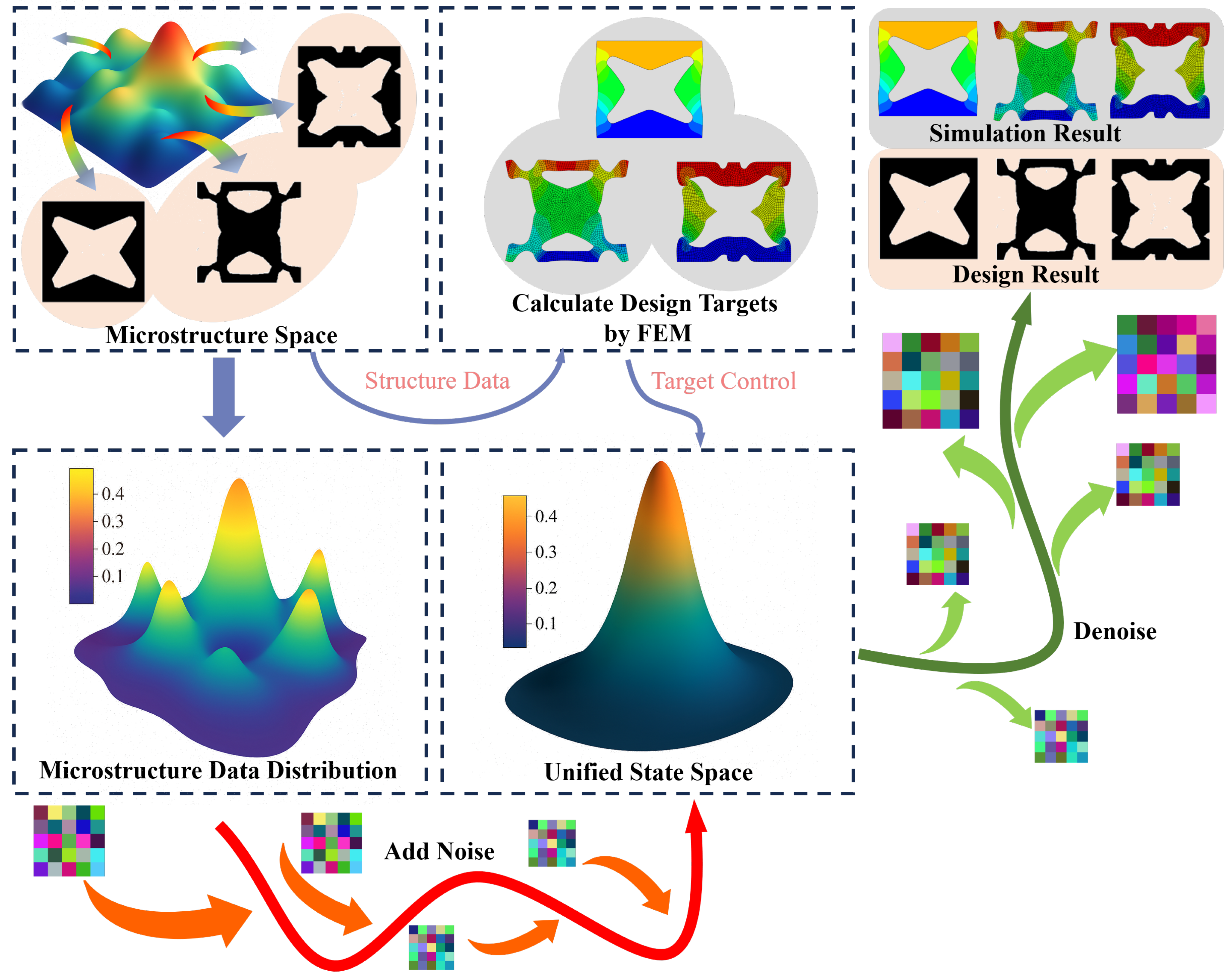
Figure 2.
Network overview and core modules of HyperDiff. (a) Denoising diffusion with a U-Net backbone. Starting from pure Gaussian noise , the model iteratively predicts and reconstructs a clear microstructure . The lower row shows the multi-scale U-Net with encoder–decoder symmetry and skip connections (red). Channel sizes and spatial resolutions are indicated as . Green blocks denote residual blocks; orange blocks denote spatial transformers; blue markers indicate max pooling / up sampling; convolutions perform channel projection. (b) Residual block (green region). Each block uses GroupNorm and SiLU activations with two convolutions, and injects the diffusion time-step via FiLM-style feature-wise modulation (time embedding → scale/shift). A residual shortcut preserves stable gradients and enables dynamic, time-aware local denoising. (c) Spatial transformer (orange region). Features are normalized, reshaped, and linearly projected, followed by self-attention and multi-head attention. The target force–displacement curve is encoded as a condition vector and fused as keys/values, enabling cross-attention guidance that propagates global mechanical constraints over the spatial field. A feed-forward network and output projection ( conv) complete the block, with residual connections for stability.
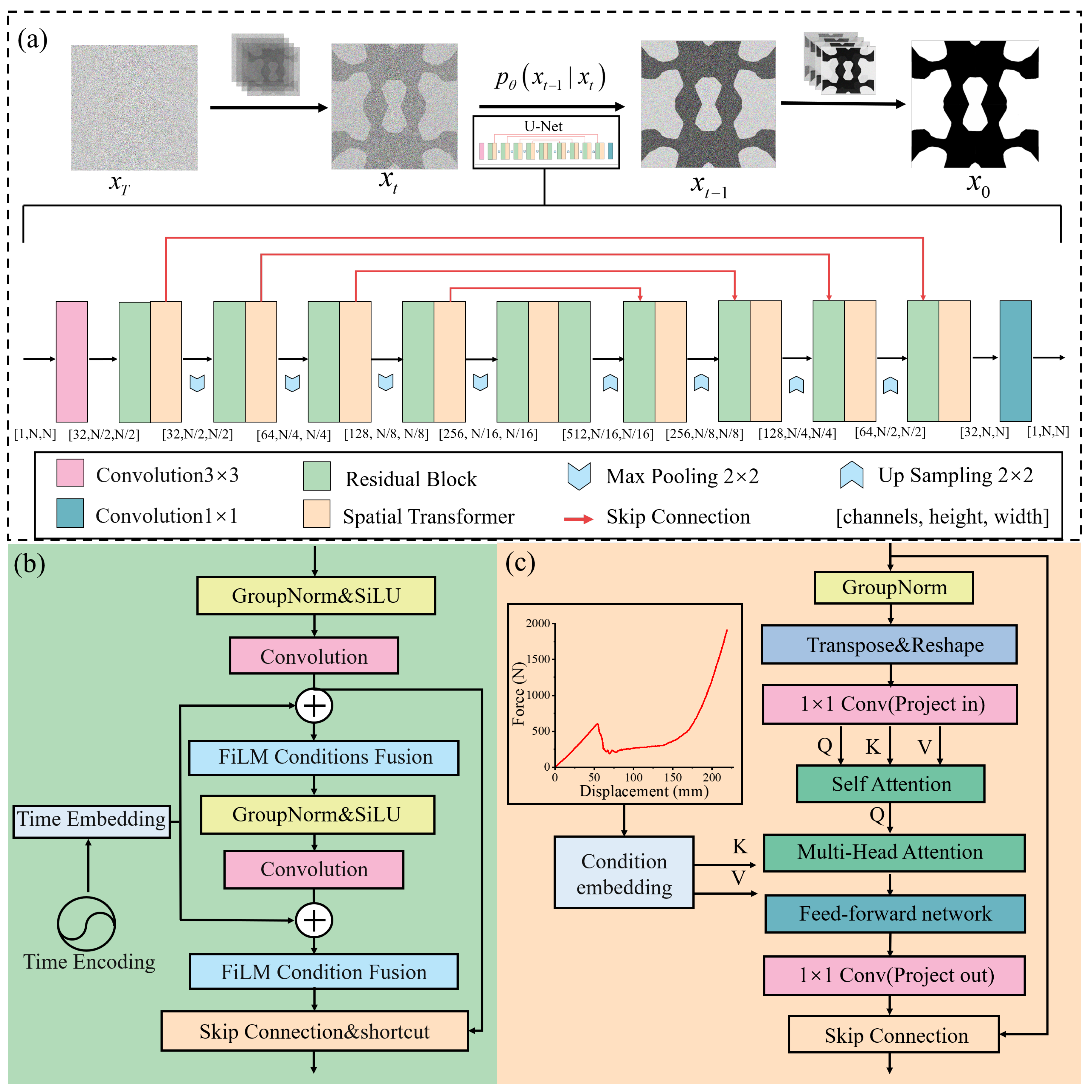
Figure 3.
Dataset construction and physical simulation framework for HyperDiff. (a) Microstructure generation based on a 2D Gaussian random field (GRF). A continuous GRF is thresholded to produce binary topologies, followed by connectivity filtering, symmetry reconstruction, and contour smoothing from rough to smooth edges. This process yields physically consistent and geometrically diverse unit cells. (b) Material calibration using uniaxial tensile tests. The TPU specimen geometry and testing setup are shown, together with the engineering, true, and fitted stress–strain curves. A second-order Ogden model accurately captures the nonlinear hyperelastic behavior. (c) Finite element simulations and force–displacement responses. Different generated microstructures are compressed under displacement control. The von Mises stress contours and corresponding force–displacement curves reveal characteristic deformation stages of elastic response, buckling, and densification. These results form a physically grounded dataset for training the conditional diffusion model.
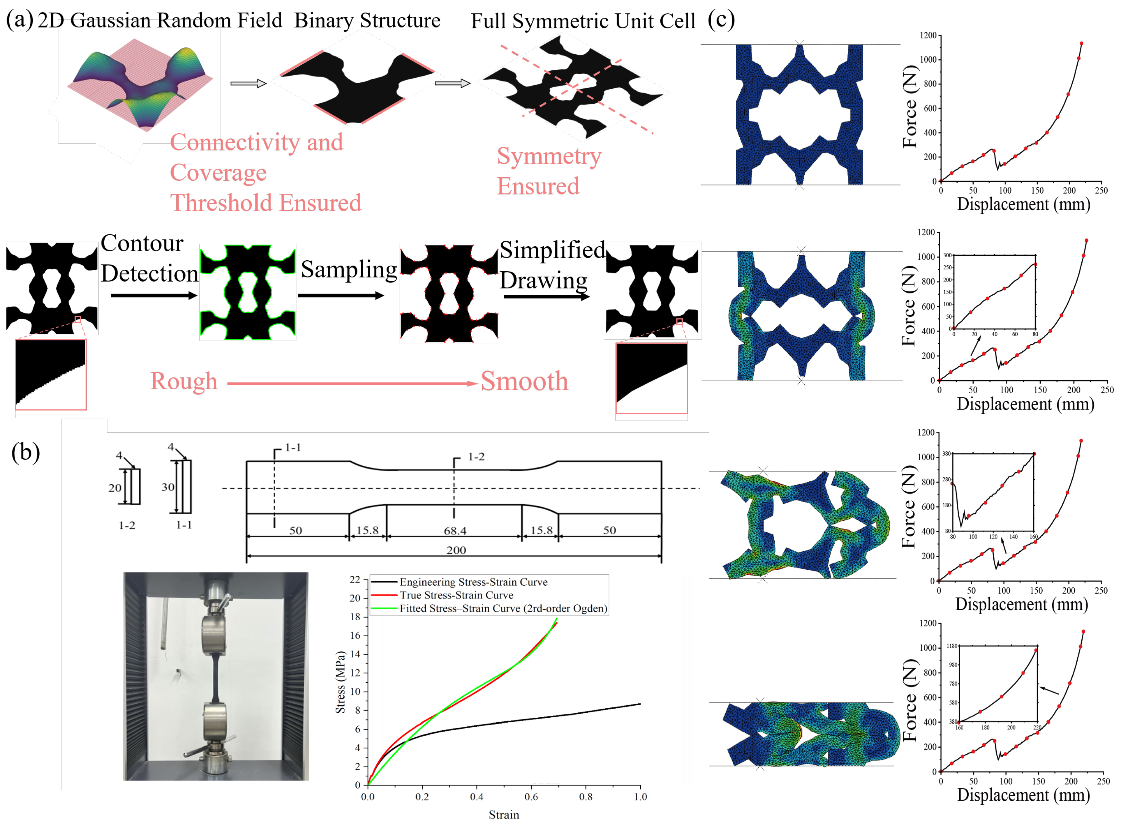
Figure 4.
Representative FE samples illustrating multi-stage deformation and response diversity (Cases 1–14). Each row shows a unique topology, its von Mises stress field under large deformation, and the corresponding force–displacement curve. The dataset spans bending-dominated compliance, buckling-induced softening (plateaus), and contact-driven densification, revealing a strongly nonconvex structure–response landscape.
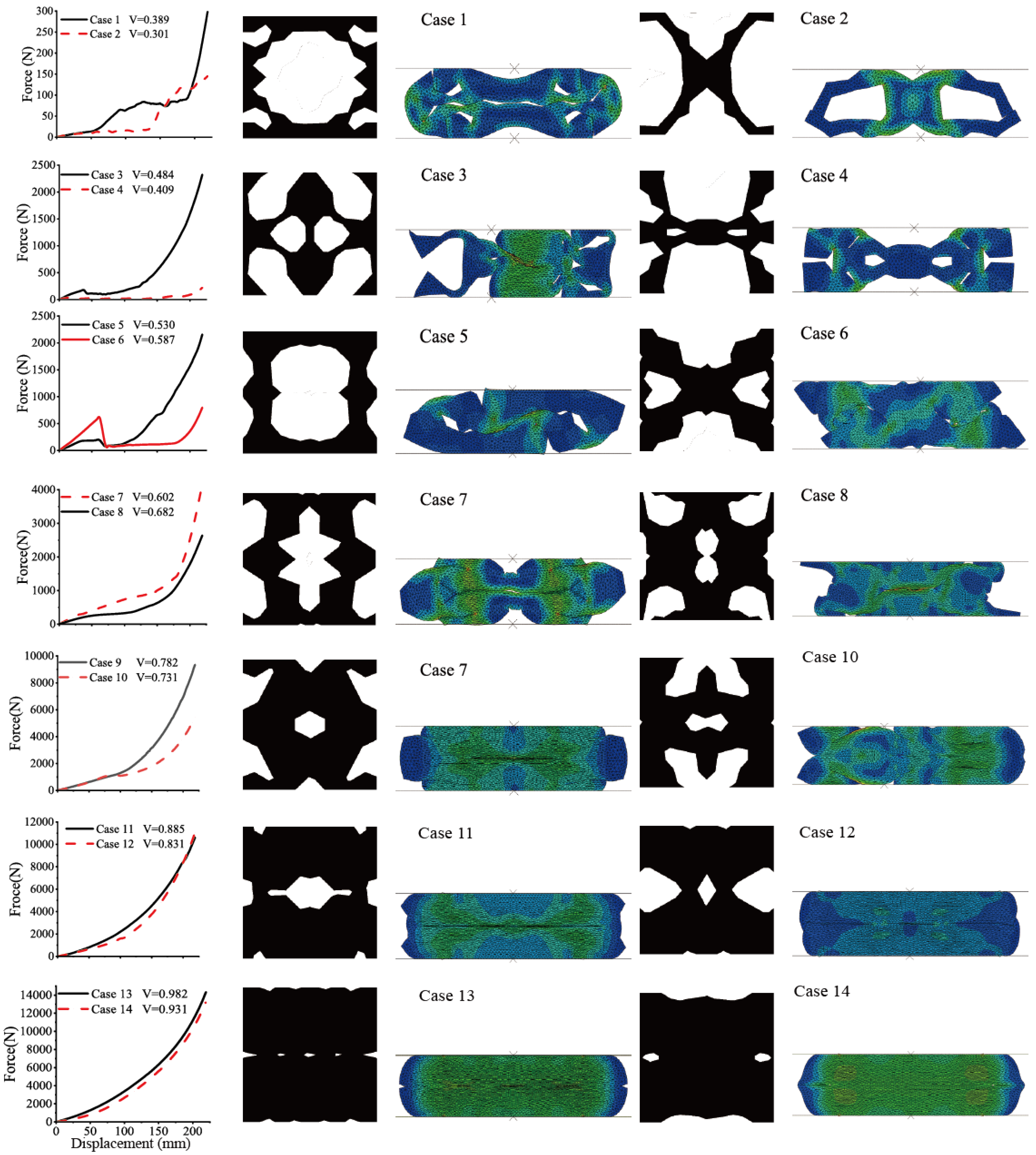
Figure 5.
Non-unique and weakly identifiable structure–property mappings (Cases 15–18).Top: distinct topologies with the same volume fraction yield markedly different force–displacement curves (mode switching under similar global descriptors). Bottom: topologies with different porosities produce nearly identical responses (one-to-many mapping). These comparisons highlight non-uniqueness, nonconvexity, and the limits of low-dimensional parametrizations, motivating a probabilistic inverse formulation.
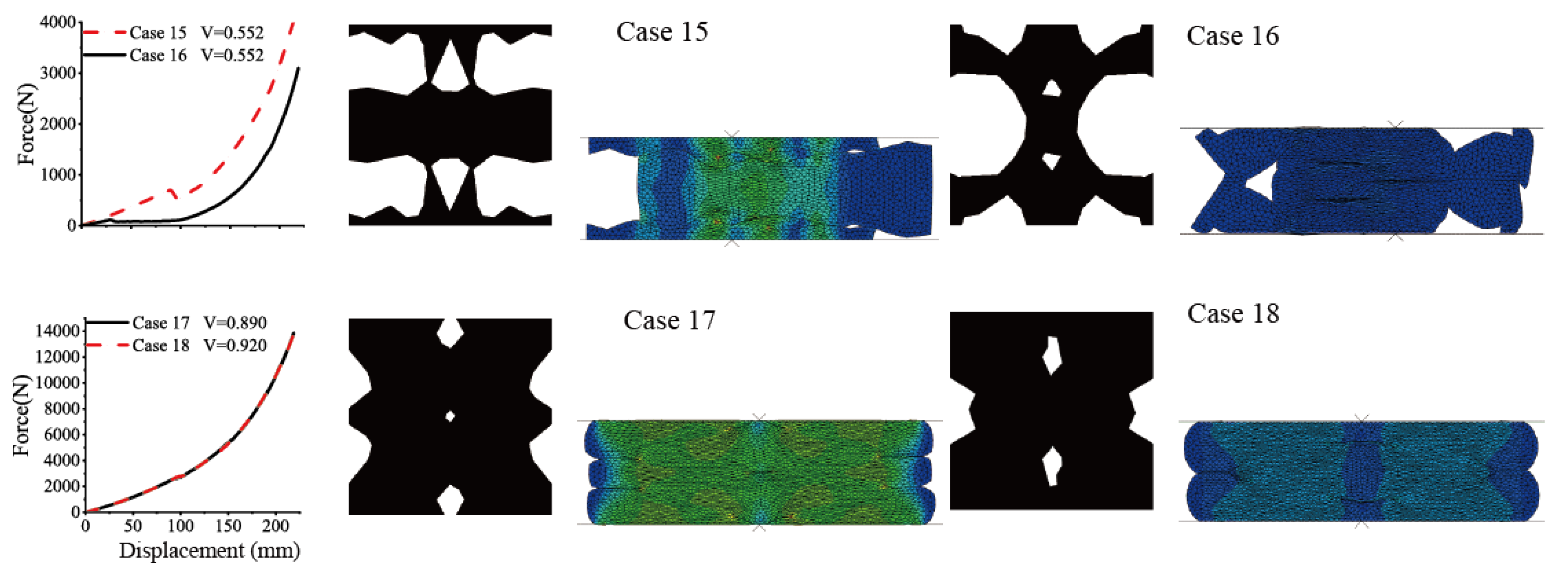
Figure 6.
Comprehensive evaluation of HyperDiff on test targets (left) and interpolated targets (right).Top row: per-case profiles of the normalized pointwise relative error along the displacement axis for four test cases (left) and four interpolated cases (right). Middle row: per-case NRMSE% distributions over 50 stochastic generations (center line = median; box = interquartile range; whiskers = 10–90th percentile). Bottom row: representative force–displacement overlays for Case 1 (left) and Interp. 1 (right); the target curve is compared to its nearest neighbor in the training set (NN-train) and the generated minimum/median samples. Legends report the corresponding percentage errors. Small topology thumbnails highlight one-to-many design diversity. Additional cases are detailed in fig:detailedresults.
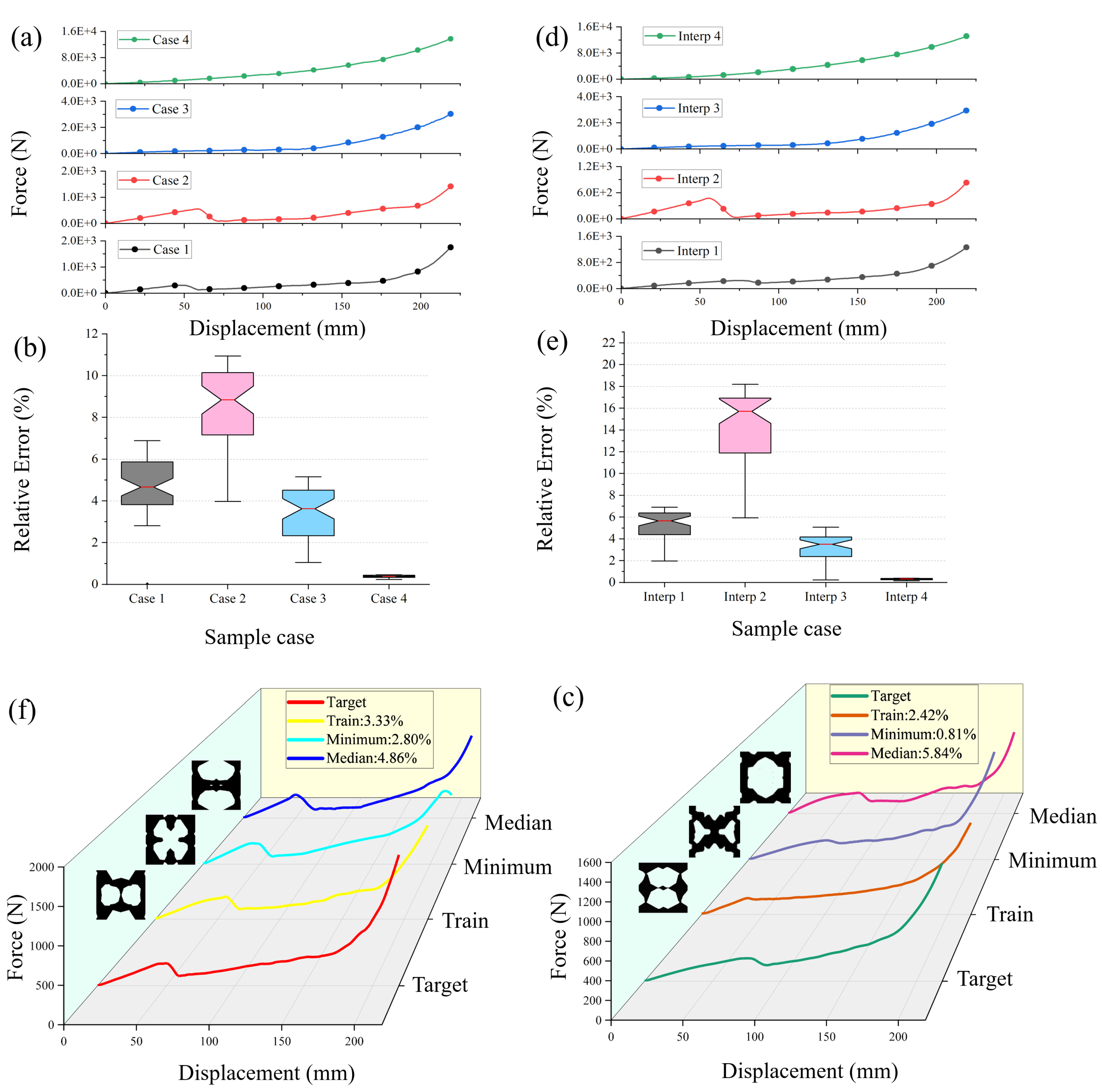
Figure 7.
Detailed overlays and corresponding topologies for the remaining test and interpolated targets. For each subfigure, the left panel shows the force–displacement overlay (Target, NN-train, Minimum, Median) with overall NRMSE%, and the three right panels show the corresponding topologies (Train, Minimum, Median).
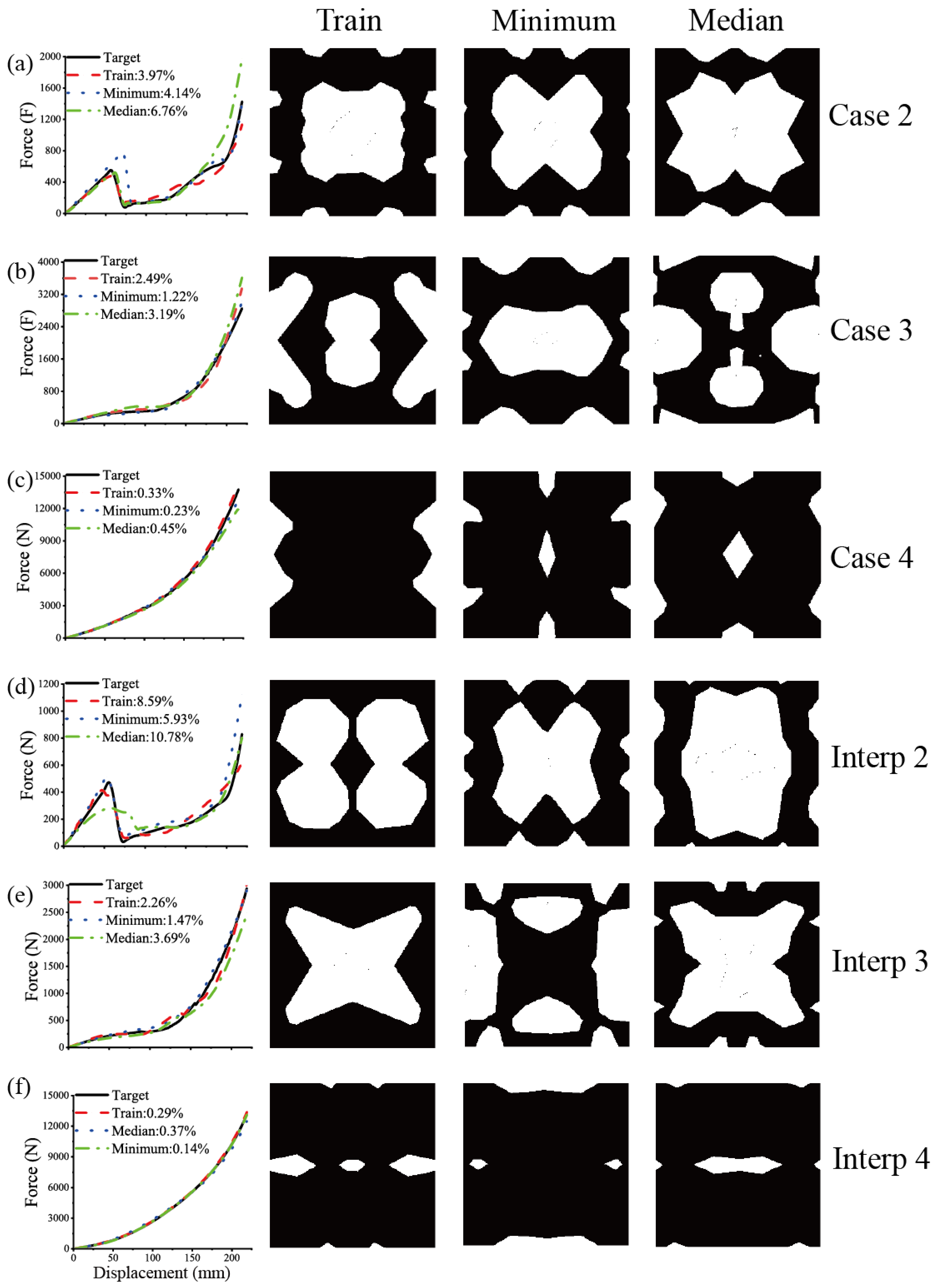
Figure 8.
Experimental verification of energy-absorbing metamaterials generated byHyperDiff. Comparison between simulation and experiment under quasi-static compression. The left panels show force–displacement curves (black dashed = target, red dotted = simulation, blue dash–dot = experiment). Vertical ticks on each curve mark six representative loading stages (I–VI) corresponding to global compression displacements and . The right panels display the corresponding deformation sequences, where the upper rows are simulated von Mises stress contours and the lower rows are experimental images. Regions of high simulated stress spatially coincide with the zones of visible large-strain localization and contact-induced densification observed in the experiments, indicating that the proposed model captures the essential deformation mechanisms and nonlinear responses of hyperelastic porous metamaterials. Here, U denotes the imposed displacement of the upper platen in millimeters (mm).
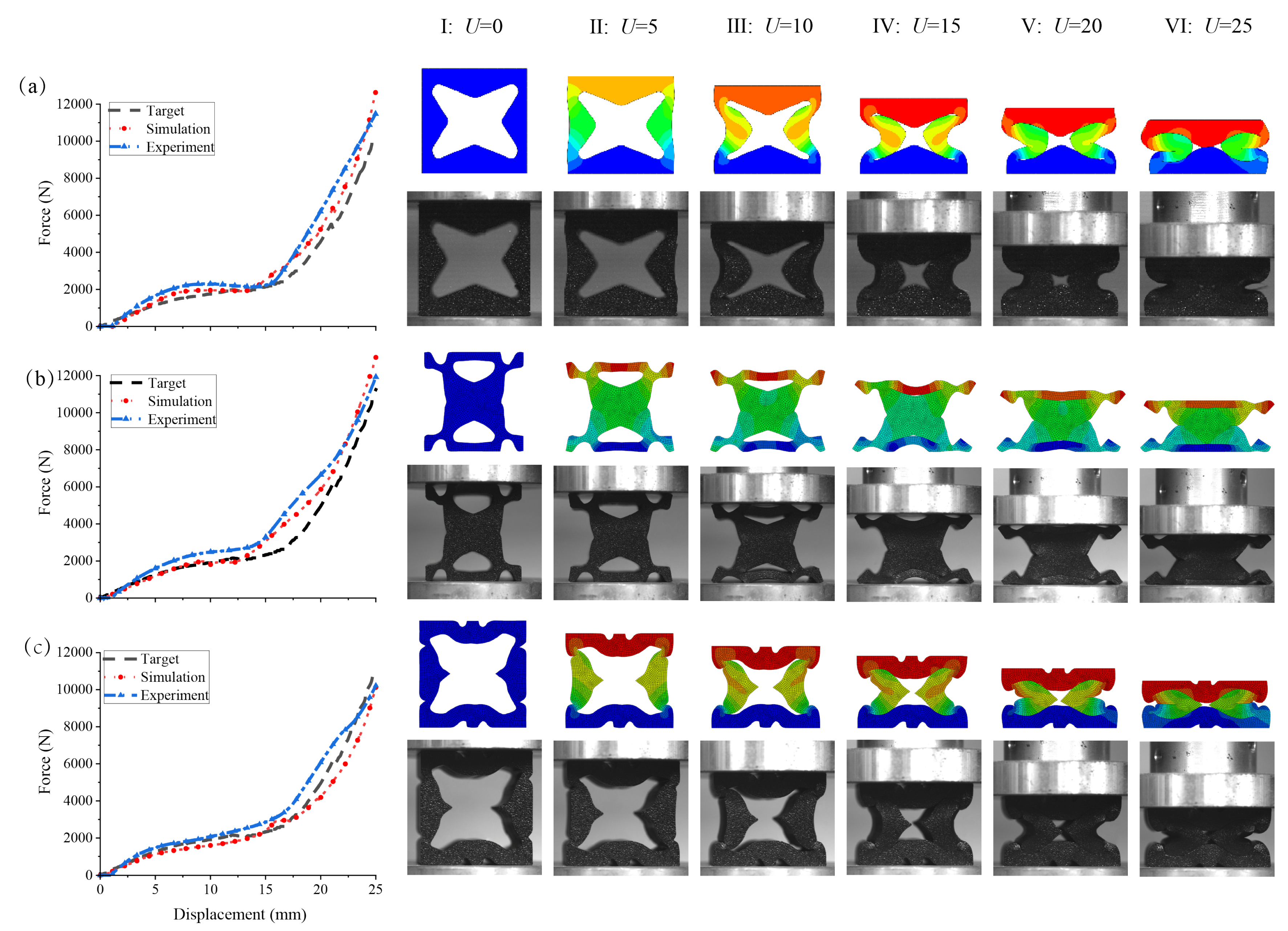

Table 1.
Fitted Ogden model parameters for the TPU material.
| Parameter | Ogden model |
|---|---|
| 12.7464 | |
| 0.0000 | |
| 0.0000 | |
| 0.0108 | |
| 12.3711 | |
| 0.0000 |
Table 2.
Key hyperparameters used for model training.
| Hyperparameter | Value |
|---|---|
| Batch size | 64 |
| Learning rate | |
| Decay steps | 25 |
| Decay factor | 0.99 |
| Input channels | 1 |
| Output channels | 1 |
| Base channels | 32 |
| Residual blocks | 1 |
| Attention layers enabled | [False, True, False, True, False] |
| Channel multipliers | [1, 1, 2, 2, 2] |
| Attention heads | 1 |
| Transformer layers | 1 |
| Condition embedding dimension | [48] |
| Noise scale range () | (1e-4, 0.02) |
| DDPM timesteps | 1000 |
| Loss function | L2 loss (MSE) |
| Image resolution | px |
| Training iterations | 100,000 |
Disclaimer/Publisher’s Note: The statements, opinions and data contained in all publications are solely those of the individual author(s) and contributor(s) and not of MDPI and/or the editor(s). MDPI and/or the editor(s) disclaim responsibility for any injury to people or property resulting from any ideas, methods, instructions or products referred to in the content. |
© 2025 by the authors. Licensee MDPI, Basel, Switzerland. This article is an open access article distributed under the terms and conditions of the Creative Commons Attribution (CC BY) license (http://creativecommons.org/licenses/by/4.0/).
Copyright: This open access article is published under a Creative Commons CC BY 4.0 license, which permit the free download, distribution, and reuse, provided that the author and preprint are cited in any reuse.


