A Neural Network Constitutive Model, and Automatic Stiffness Evaluation for Multiscale Finite Elements

1. Introduction

Multiscale modeling is a simulation technique that describes a behavior at a given length scale based on the physics at a finer scale, which in turn is considered to be better known or easy to be modeled. Structures made of composite materials or materials with microstructure constitute typical candidates for multiscale modeling. In fact, it is impossible to model a whole structure by taking all constituents and their, possibly nonlinear interactions within the model. Therefore, a compromise must be considered, where a reduction in precision and an increase in uncertainty related to multiscale modeling should be accepted, to avoid the complexity of a full-scale model. In engineering, homogenization is a representative example of applied multiscale modeling [1]. In linear problems, homogenization is usually based on analytical expressions that give the homogenized properties for a given microstructure or composite material [2,3]. This approach is powerful, despite certain theoretical difficulties for the calculation of homogenized properties. Numerical homogenization allows for the extension of classical analytical homogenization in order to describe more complicated problems. Homogenized properties are load-dependent or even path-dependent; therefore, analytical solutions are difficult to calculate orxist. A path-independent problem is considered here as a first example.

Artificial neural networks have been applied in different areas of science and engineering, where data sets are available for training and testing. In particular, ANNs are employed in elastoplastic and contact problems in mechanics by using a minimization of energy. The Hopfield and Tank neural networks have been proposed by Kortesis and Panagiotopoulos [4], and Avdelas et al. [5]. The feedforward NNs trained by the backpropagation algorithm have been used for an approximation of several problems in mechanics based on examples (supervised learning). Inverse and parameter-identification problems in mechanics have been solved by using backpropagation neural networks in Stavroulakis et al. [6,7], Stavroulakis [8], Waszczyszyn and Ziemianski [9]. The buckling loads in non-linear problems for elastic plates have been calculated by neural netwoks in Muradova and Stavroulakis [10]. A recent review of the classical usage of neural networks within computational mechanics has been published by Yagawa and Oishi [11].

Several neural network-based constitutive models have been proposed in recent works. The main directions are described in the review article of Dornheim et al. [12].

The workdescribed here belongs to the more general topic of CANN (constitutive artificial neural network). In fact from input-output relations an artificial neural network is able to learn and replace a mathematically consistent constitutive material model. Adding of additional information, like thermomechanical restrictions, enhances the effectiveness and allows for training with less data. Further information can be found, among others, in references [12,13,14].

Here an efficient way to store the constitutive relation based on a data-base of responses of a representative volume element (RVE) is proposed through a construction of a neural network constitutive surrogate model. Subsequently, usage of this surrogate within a nonlinear, upper level finite element model, is straightforward.

For fitting in the backpropagation a model from the representative volume element has been taken. The target and test data has been collected from the numerical experiments. The data set from the responses of representative volume elements is divided into training ($50\%$) and test data ($50\%$). In addition, a data set from a nonlinear polynomial constitutive model for hyperelastic materials is tested. The numerical results obtained from the constructed neural network are compared with the exact values at the predicted points.

An artificial neural network together with the method of automatic differential of Tensorflow-scientific library in Python programming [15] is used here. The neural model includes the automatic differentiation [16] for calculating partial derivatives of the ANN output, i.e. components of the tangential stiffness tensor. Calculating stiffness matrix, i.e. partial derivatives of the stress function helps to improve the results of an approximation of the stress function. The automatic differentiation is performed through the chain rule, applied to the neural stress models and then in the residual model except of fitting the data set of the stress tensor, fitting the given stiffness matrix, obtained from the representative volume elements, is provided as well. That helps to get more accurate neural surrogate models for the stress tensor components. The predicted results are compared with calculated data for the stress tensor. The ANN is trained with different error loss functions. The Sobolev metrics [17] is also tested in a minimization problem. The proposed neural model allows a prediction of the material response from the strain effects. Numerical examples of creating the neural nonlinear model and computing of stresses and its first derivatives, based on data set $\{{\mathsf{\epsilon }}_i,{\mathsf{\sigma }}_i,i=1,2,...,N\}$ in composite structures are considered.

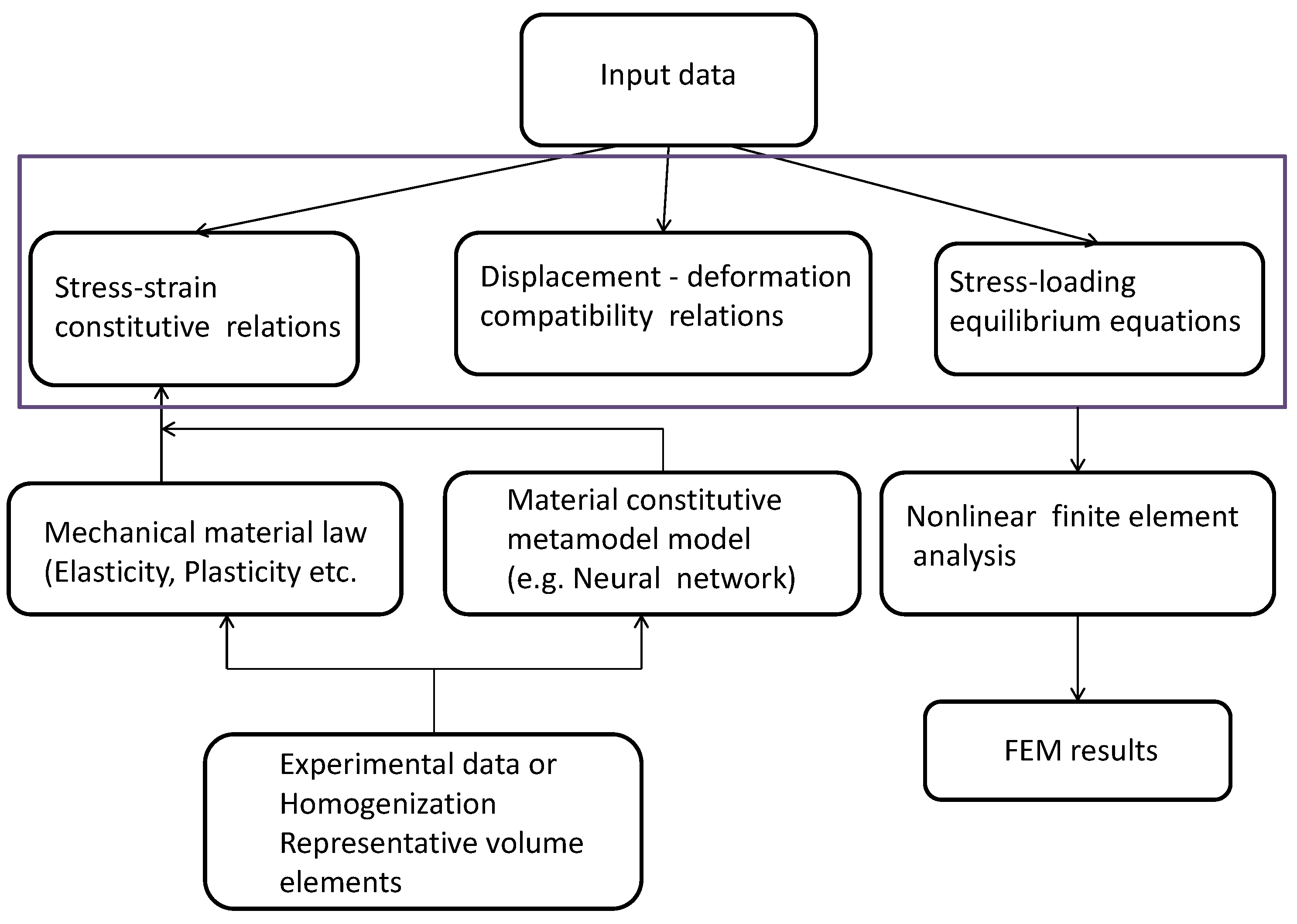
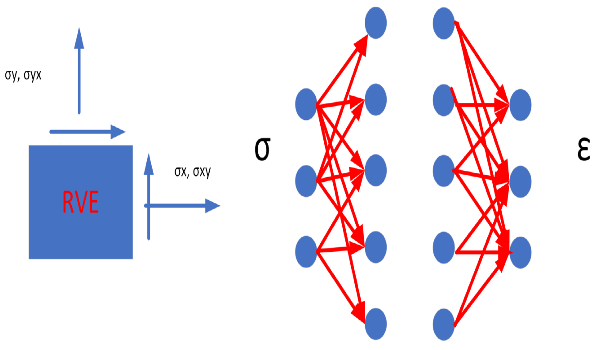
2. Background of the Constitutive Metamodel, Based on Responses of Representative Volume Elements

Analytical homogenization replaces a RVE with several materials (composite) or microstructure with a continuum with homogenized properties [18,19]. In a nonlinear behavior this step must be repeated for each level of stress resp. strain. Nevertheless, this approach has been followed and gives a multi-scale technique, which has been called FEM2 [20]. The method is accurate, but requires enormous resources, due to the need of solving the detailed model of the RVE for every different combination of loadings that appear during incremental-iterative solution of the homogenized finite element model.

Classical polynomial surrogates as well as a neural network and other ones have been proposed and tested in [1,21,22,23,24,25,26,27,28].

A feedforward neural network has the ability to correlate vector inputs with vector outputs, provided that the parameters involved have been suitably calculated. This step is done with the help of data (examples) within a step called training. The topology of the neural network (number of layers and neurons) as well as the activation functions (basis functions) at nodes in correlation with the number of examples define the ability of the network to approximate well an unknown target function. Trial and error or optimal design principles can be used towards a satisfactory result [29].

A modern approach for introducing physics into the neural network metamaterial uses differential equations of mechanics in combination with automatic differentiation of output of the neural network, in order to train the network, without using specific input-output sample examples. This is so-called physics-informed neural networks approach ([15,28,30,31,32,33], etc.). Within the homogenization metamodel PINN could provide thermomechanicaly consistent approximations that are more stable with respect to blind neural network ones.

Usage of artificial neural networks is able to simulate classical mechanical problems, if sufficient samples of input-output data are provided for training. The concept is shown schematically in Figure 1 and Figure 2 ([1]) for the stress-strain relation of the RVE. The RVE for every possible complexity is solved for different combinations of stresses and the corresponding strains are calculated and used for training. More refined approaches introduce additional physical restrictions on the corresponding constitutive metamodel, so that thermomechanical principles are not violated [28]. Furthermore, loading sequences can be used in a path-dependent problem, in order to train a corresponding neural network that will provide the response based on previous loading sequences at a given point.

The trained neural network can be integrated into a finite element program and replaces the required constitutive response, as it is outlined in Figure 1 (see, among others, [1,2,34,35]). The material constitutive law is based on experimental or RVE data. It is based either on an established mechanical material law or a metamodel (interpolation), for example, a neural network one. This approach is close to the classical usage of constitutive relations and can be integrated with existing commercial finite element packages [36,37,38,39].

The results used here correspond to a masonry structure with different stones and mortar materials and submected to various stress-strain levels. The Representative Volume Element has been discretized by the finite element method. Results are collected in a data-base, which is used for training of the neural network. A MATLAB implementation for multi-scale analysis of two-dimensional problems as well as the database is available as supplementary material to reference [1]. The masonry RVE used for the creation of the data-base. The plastic deformations calculated under one strain loading are shown in Figure 3 ([1]), both taken from reference [40].

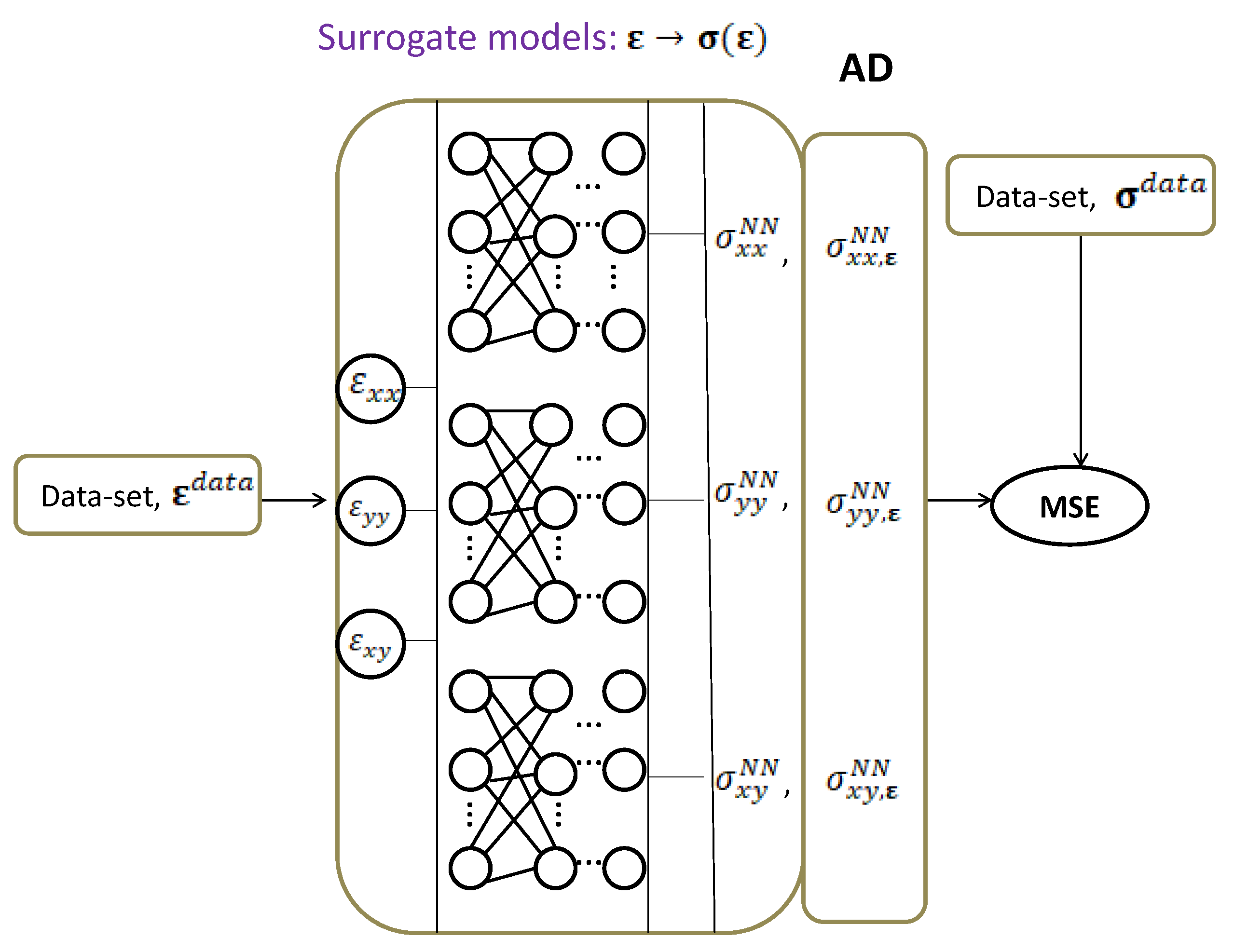
3. Feedforward and Backpropagation in the Neural Model with a Computation of Tangential Stiffness Matrix

A computational approach initially proposed and presented in [1] uses two neural network metamodels, one for the approximation of the constitutive relation and the second one for the approximation of it’s first derivative, i.e. the calculation of the tangential stiffness matrix. Here, following ideas from PINN’s community, we construct a neural network on the base of scientific software Tensorflow with possibilities of automatic differentiation for calculating partial derivatives as well.

The experimental data for the components of the stress and strain tensors are used in order to construct a neural network model which expresses nonlinear constitutive relations $\mathsf{\sigma }=\mathsf{\sigma }\left(\mathsf{\epsilon }\right)$. Three neural surrogate models, intended for computing components of the stress tensor, ${\sigma }_{xx},$${\sigma }_{yy}$ and ${\sigma }_{xy}({\sigma }_{yx}={\sigma }_{xy})$ are proposed, respectively. Namely, there are three ANNs with three inputs, strain components ${\epsilon }_{xx},$${\epsilon }_{yy}$ and ${\epsilon }_{xy}({\epsilon }_{yx}={\epsilon }_{xy})$ and one output which is a component of the stress tensor, i.e. the first NN has output ${\sigma }_{xx}^{NN}$, the second one has output ${\sigma }_{yy}^{NN}$ and the third one has output ${\sigma }_{xy}^{NN}$. The architecture of the proposed bundle of NNs is presented in Figure 4.

In feedforward of the neural network the output vector from each layer is calculated as follows

$$\begin{array}{ccc}\hfill z_0& =& {({\mathsf{\epsilon }}_{11},{\mathsf{\epsilon }}_{22},{\mathsf{\epsilon }}_{12})}^T,\hfill \end{array}$$

(1)

$$\begin{array}{ccc}\hfill z_k& =& f(W_k^T{z}_{k-1}+b_k),k=1,2,...,N_L-1,\hfill \\ \hfill {\sigma }_{ij}^{NN}=z_{N_L}& =& W_{N_L}^T{z}_{N_L-1}+b_{N_L},i,j=1,2,\hfill \end{array}$$

(2)

where ${\mathsf{\epsilon }}_{11}={\mathsf{\epsilon }}_{xx},{\mathsf{\epsilon }}_{12}={\mathsf{\epsilon }}_{21}={\mathsf{\epsilon }}_{xy}={\mathsf{\epsilon }}_{yx},{\mathsf{\epsilon }}_{22}={\mathsf{\epsilon }}_{yy},$$W_k^T$ is the matrix of the dimension $(n_{k-1}\times n_k)$, containing the weights between $k-1$ and k hidden layers with $n_{k-1}$ and $n_k$ neurons, respectively. The $W_N^T$ is the matrix containing the weights between the last hidden layer and the output of the neural network. The $b_k$ are biases. There is no activation function f for the output layer in Keras module, but the tf.keras.layers.Activation function can be used to apply a custom activation function to the output, for example, tf.keras.layers.Activation(tf.nn.relu)

The residual part $MSE$ (mean square error) can be trained by two approaches. In the first approach the error function for each output is minimized separately. This can be done because the components of the stress tensor are computed independently. However, the residuals of the outputs can also be treated together, simultaneously. In the second approach the computations are less expensive, in terms of time and number of iterations, in comparison to the first approach.

The residual parts are computed as

$$MSE=MS{E}_{\sigma }+MS{E}_S,$$

(3)

where $MS{E}_{\Sigma }$ is the loss error function while training the data for the strain and stress tensor and $MS{E}_S$ is the Sobolev loss error function [17], i.e error function for the derivatives if these data are available. The residual $MS{E}_{\sigma }$ is written as

$$MS{E}_{\sigma }={\displaystyle \frac{1}{N}}\sum _{i=1}^N\left|\right|{\mathsf{\sigma }}_i^{NN}-{\mathsf{\sigma }}_i^{\mathrm{data}}\left|\right|,$$

(4)

where $\left|\right|·\left|\right|$ is the Euclidean norm, ${\mathsf{\sigma }}_i^{NN}={\mathsf{\sigma }}^{NN}\left({\mathsf{\epsilon }}_i\right)=[{\sigma }_{xx}^{NN}\left({\mathsf{\epsilon }}_i\right),{\sigma }_{yy}^{NN}\left({\mathsf{\epsilon }}_i\right),{\sigma }_{xy}^{NN}\left({\mathsf{\epsilon }}_i\right)]$ are the output of the neural network, namely, the values of the stress tensor which are computed by the composed constitutive neural network of the variable data set ${\mathsf{\epsilon }}_i={[{\epsilon }_{xx},{\epsilon }_{yy},{\epsilon }_{xy}]}_i$ and N is the number of the values for fitting the given data set for the stress tensor (samples). If the residuals for the surrogate models, ${\sigma }_{xx}^{NN}\left({\mathsf{\epsilon }}_i\right),$${\sigma }_{yy}^{NN}\left({\mathsf{\epsilon }}_i\right),$${\sigma }_{xy}^{NN}\left({\mathsf{\epsilon }}_i\right)$ are treated separately then instead of (4) the following formulas yield

$$\begin{array}{c}\hfill MS{E}_{{\sigma }_{ij}}={\displaystyle \frac{1}{N}}\sum _{k=1}^N|{\sigma }_{ij,k}^{NN}-{\sigma }_{ij,k}^{\mathrm{data}}|,i,j=1,2,\\ \hfill {\sigma }_{11}={\sigma }_{xx},{\sigma }_{12}={\sigma }_{21}={\sigma }_{xy}={\sigma }_{yx},{\sigma }_{22}={\sigma }_{yy}\end{array}$$

(5)

and in Figure 4 we have three $MSE{\sigma }_{11}$, $MSE{\sigma }_{22}$ and $MSE{\sigma }_{12}$ for each surrogate neural network, respectively.

In case of the Sobolev metrics in the neural network [17] the derivative information can easily be incorporated into training process of the neural network model for $\mathsf{\sigma }$ by making derivatives of the neural network match the ones given by $\mathsf{\sigma }$.

If we have access to the partial derivatives of the stress tensor $\mathsf{\sigma }$ with respect to the input $\mathsf{\epsilon }$ till k order.

$${\{{\mathsf{\epsilon }}_i,\mathsf{\sigma }\left({\mathsf{\epsilon }}_i\right),D_{\mathsf{\epsilon }}^1\left(\mathsf{\sigma }\left({\mathsf{\epsilon }}_i\right)\right),...,D_{\mathsf{\epsilon }}^K\left(\mathsf{\sigma }\left({\mathsf{\epsilon }}_i\right)\right)\}}_i^N,$$

where $D_{\mathsf{\epsilon }}^k\left(\mathsf{\sigma }\left({\mathsf{\epsilon }}_i\right)\right)={\left({\partial }^k\mathsf{\sigma }/\partial {\mathsf{\epsilon }}^k\right)}_i,$$k=1,2,...,K$ and $D_{{\epsilon }_{kl}}^1{\sigma }_{ij}=D_{{\epsilon }_{ij}}^1{\sigma }_{kl}$ then the Sobolev error loss function $MS{E}_S$ can be included as well in (4), i.e.

$$MSE={\displaystyle \frac{1}{N}}\sum _{i=1}^N\left(\left|\right|{\mathsf{\sigma }}_i^{NN}-{\mathsf{\sigma }}_i^{\mathrm{data}}\left|\right|+\sum _{k=1}^K\sum _{i=1}^N\left|\right|D_{\mathsf{\epsilon }}^k\left({\mathsf{\sigma }}_i^{NN}\left(\mathsf{\epsilon }\right)\right)-D_{\mathsf{\epsilon }}^k\left({\mathsf{\sigma }}_i^{\mathrm{data}}\right)\left|\right|\right),$$

(6)

or in virtue of (5),

$$\begin{array}{c}\hfill MS{E}_{ij}={\displaystyle \frac{1}{N}}\sum _{k=1}^N|{\mathsf{\sigma }}_{ij,k}^{NN}-{\mathsf{\sigma }}_{ij,k}^{\mathrm{data}}|+\sum _{k=1}^K\sum _{i=1}^N|D_{\mathsf{\epsilon }}^k\left({\mathbf{\sigma }}_{ij,k}^{NN}\left(\mathsf{\epsilon }\right)\right)-D_{\mathsf{\epsilon }}^k\left({\mathbf{\sigma }}_{ij,k}^{\mathrm{data}}\right)|.\end{array}$$

(7)

The numerical experiments have shown that the results are improved after using the Sobolev function. Since the process of numerical differentiation is not stable in order to get a good accuracy for computations of the derivatives a lot of training iterations are needed. With small perturbations (errors) in the output of the neural network (components of the stress tensor) one can get a quite large error for the derivatives of the components. The Sobolev training can overcome these disadvantages by matching the derivatives of the output of NN. Then the rate of convergence is higher and a good accuracy can be reached quickly.

In backpropagation the chain rule from calculus is used to compute the gradients. The output of a NN is considered as a composite function, therefore its derivative is equal to the product of the derivatives of its individual components. In the context of backpropagation, this means that the gradients of the loss with respect to the weights of a given layer depend on the gradients of the loss with respect to the weights of the subsequent layer. Once the gradients have been computed, they are used to update the weights of the network using optimization algprithm (e.g. gradient descent). The optimization method adjusts the weights in the direction that minimizes the loss, allowing the network to improve its performance.

The target solution is presented through expansion from basis (sigmoid, hyperhyperbolic tangent etc.) functions. The network is trained iteratively on a set of input-output ($\mathsf{\epsilon }$, $\mathsf{\sigma }$) data, the weights are updated, and the process is repeated until the network has learned to produce accurate outputs for a wide range of inputs. One of the advantages of backpropagation is that it allows neural networks to learn from their mistakes and improve their performance over time. This is particularly useful in applications where the relationship between the inputs and outputs is nonlinear (e.g. in macrostructures). However, the procedure of backpropagation can be computationally expensive, particularly for large networks and when the network becomes too complex and starts to fit the training data too closely, leading to poor performance on new, unseen data.

Automatic differentiation (AD) method, built in Tensorflow library, computes exact gradients using the chain rule, resulting in more accurate derivatives in comparison with finite differences. In backpropagation the gradients are computed with respect to the weights and the biases. The derivatives of the output function is also computed by using AD through chain rule with respect to input variables. However, since the output of the neural network is an approximation of the exact solution, i.e. the output data have some perturbation with the AD this perturbation (error) will not decrease and more likely increases. The results of computing of the derivatives by the AD can be compared with an numerical differentiation, e.g. FD approximation (forward, backward and central) or with some other well known numerical methods for numerical differentiation. For the error of approximation, for example, of the forward differences for the partial derivatives for the $\mathsf{\sigma }$ we have

$$\begin{array}{c}\hfill D_{{\epsilon }_{11}}^1{\sigma }_{ij}={\displaystyle \frac{{\sigma }_{ij}({\epsilon }_{11}+\Delta {\epsilon }_{11},{\epsilon }_{22},{\epsilon }_{12})-{\sigma }_{ij}\left(\mathsf{\epsilon }\right)}{\Delta {\epsilon }_{11}}}+O\left(\Delta {\epsilon }_{11}\right),\end{array}$$

(8)

$$\begin{array}{c}\hfill D_{{\epsilon }_{22}}^1{\sigma }_{ij}={\displaystyle \frac{{\sigma }_{ij}({\epsilon }_{11},{\epsilon }_{22}+\Delta {\epsilon }_{22},{\epsilon }_{12})-{\sigma }_{ij}\left(\mathsf{\epsilon }\right)}{\Delta {\epsilon }_{22}}}+O\left(\Delta {\epsilon }_{22}\right),\end{array}$$

(9)

$$\begin{array}{c}\hfill D_{{\epsilon }_{12}}^1{\sigma }_{ij}={\displaystyle \frac{{\sigma }_{ij}({\epsilon }_{11},{\epsilon }_{22},{\epsilon }_{12}+\Delta {\epsilon }_{12})-{\sigma }_{ij}\left(\mathsf{\epsilon }\right)}{\Delta {\epsilon }_{12}}}+O\left(\Delta {\epsilon }_{12}\right).\end{array}$$

(10)

If the output of the neural network has an error ${\mathbf{\delta }}^{NN}={\mathsf{\sigma }}^{NN}-\mathsf{\sigma }$ then

$$\begin{array}{c}\hfill D_{{\epsilon }_{11}}^1{\sigma }_{ij}^{NN}-D_{{\epsilon }_{11}}^1{\sigma }_{ij}={\displaystyle \frac{{\delta }_{ij}^{NN}({\epsilon }_{11}+\Delta {\epsilon }_{11},{\epsilon }_{22},{\epsilon }_{12})-{\delta }_{ij}^{NN}\left(\mathsf{\epsilon }\right)}{\Delta {\epsilon }_{11}}}+O\left(\Delta {\epsilon }_{11}\right),\end{array}$$

(11)

$$\begin{array}{c}\hfill D_{{\epsilon }_{22}}^1{\sigma }_{ij}^{NN}-D_{{\epsilon }_{22}}^1{\sigma }_{ij}={\displaystyle \frac{{\delta }_{ij}^{NN}({\epsilon }_{11},{\epsilon }_{22}+\Delta {\epsilon }_{22},{\epsilon }_{12})-{\delta }_{ij}^{NN}\left(\mathsf{\epsilon }\right)}{\Delta {\epsilon }_{22}}}+O\left(\Delta {\epsilon }_{22}\right),\end{array}$$

(12)

$$\begin{array}{c}\hfill D_{{\epsilon }_{12}}^1{\sigma }_{ij}^{NN}-D_{{\epsilon }_{12}}^1{\sigma }_{ij}={\displaystyle \frac{{\delta }_{ij}^{NN}({\epsilon }_{11},{\epsilon }_{22},{\epsilon }_{12}+\Delta {\epsilon }_{12})-{\delta }_{ij}^{NN}\left(\mathsf{\epsilon }\right)}{\Delta {\epsilon }_{12}}}+O\left(\Delta {\epsilon }_{12}\right).\end{array}$$

(13)

Thus,

$$\left|\right|D_{\mathsf{\epsilon }}^1{\mathsf{\sigma }}^{NN}-D_{\mathsf{\epsilon }}^1\mathsf{\sigma }\left|\right|=O\left({\displaystyle \frac{\left|\right|{\mathbf{\delta }}^{NN}{\left|\right|}_{\infty }}{\mathbf{ϵ}}}\right)+{O\left(\right|\left|\Delta \mathsf{\epsilon }\right||}_{\infty }),$$

(14)

where $\left|\right|D_{\mathsf{\epsilon }}^1{\mathsf{\sigma }}^{NN}-D_{\mathsf{\epsilon }}^1\mathsf{\sigma }\left|\right|$ is the Euclidean norm, $\left|\right|{\mathbf{\delta }}^{NN}{\left|\right|}_{\infty }={max}_{ij}\left|{\delta }_{ij}^{NN}\right|,$$\mathbf{ϵ}={min}_{ij}\left|\Delta {\mathsf{\epsilon }}_{ij}\right|,$ ${\left|\right|\Delta \mathbf{\epsilon }\left|\right|}_{\infty }={max}_{ij}\left|\Delta {\mathsf{\epsilon }}_{ij}\right|.$ For the backward the same estimate is true. Analogously, for the central differences we obtain

$$\left|\right|D_{\mathsf{\epsilon }}^1{\mathsf{\sigma }}^{NN}-D_{\mathsf{\epsilon }}^1\mathsf{\sigma }\left|\right|=O\left({\displaystyle \frac{\left|\right|{\mathbf{\delta }}^{NN}{\left|\right|}_{\infty }}{\mathbf{ϵ}}}\right)+{O\left(\right|\left|\Delta \mathsf{\epsilon }\right||}_{\infty }^2).$$

(15)

Hence, one concludes that the error of numerical differentiation can increase much if the perturbation $\left|\right|{\mathbf{\delta }}^{NN}{\left|\right|}_{\infty }$ is big. One can compare the values of the derivatives, computed from the neural model with the use of AD with the approximated derivatives, computed by the FD.

According to the results, presented in [41] for a common class of artificial neural networks with one hidden layer, the mean integrated squared error between the estimated network and a target function $\sigma$ is bounded by

$$O\left({\displaystyle \frac{C_{\sigma }^2}{n}}\right)+O\left({\displaystyle \frac{nd}{N}}logN\right),$$

(16)

where n is the number of neurons in the hidden layer, d is the input dimension, N is the number of training observations (samples), and $C_{\sigma }$ is the first absolute moment of the Fourier magnitude distribution of the target function $\sigma$, i.e. $C_{\sigma }$ quantifies the regularity of the function via an integral involving the Fourier transform, (see Formula (2) [41]). There are the two contributions to this total risk, the approximation error and the estimation error. The approximation error is the distance between the target function and the closest neural network function of a given architecture and estimation error refers to the distance between this ideal network function and an estimated network function. The constant $C_{\sigma }$ can be exponentially large in d for sequences of functions $\sigma$ of increasing dimensionality. The networks with many hidden layers may improve the accuracy in some cases.

From the formulas (14), (15) and the estimate (16) one concludes that the error of neural network influences the total estimate of the error of computation of the derivatives of the output function. However, with AD the computations are more accurate because of the derivatives are computed exactly by the chain rule.

Since the tangent stiffness matrix is symmetric, only the components, located in the lower or upper triangular parts of this matrix can be used and thereby decrease the time of computations. Here in feedforward the nonlinear tahn activation function is used, which provides better approximation in comparison with the other activation functions. In the backpropagation usually, the weights and biases are updated using a stochastic optimizer, such as the Stochastic Gradient Descent (SGD) and Adam’s method [42]. The residual network updates the surrogate networks’ weights and biases using the residual obtained from the residual network. Here we use the Adam optimize algorithm.

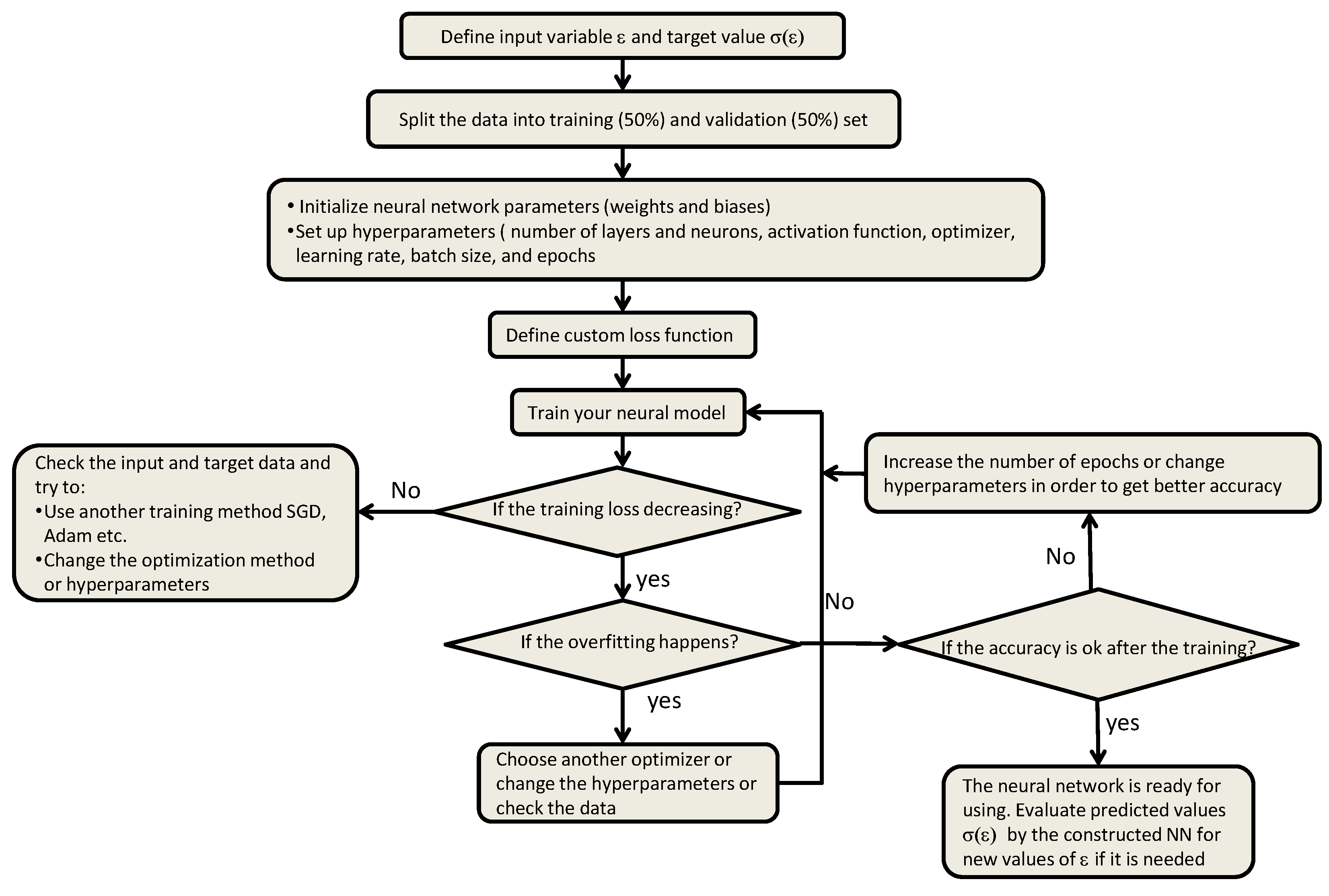
4. Computational Procedure

In this section a computational algorithm for constructing a neural network constitutive metamodel is presented. The procedure is implemented with the use of automatic differentiation of Tensorflow and Keras library of Python [43]. In order to optimize weights and biases the Adam’s optimization algorithm is applied and the training set is divided into butches. The flowchart summarizing the process of constructing of a neural network is presented on Figure 5

The steps of implementation of the procedure with some methods/functions of the Python programming code are described below.1

• Import all necessary Python’s libraries: import tensorflow as tf, import keras, import matplotlib.pyplot as plt, import csv.
  (There are three distinct parts that define the TensorFlow: workflow, preprocessing of data, building the model, and training the model to make predictions.
  The Keras library is an open-source library of the TensorFlow platform that provides a Python interface for creation of artificial neural networks.
  Matplotlib is a library for creating static, animated, and interactive visualizations in Python. With Matplotlib.pyplot some plots are created in the code.
  The library csv allows writing and reading data in the CSV (Comma Separated Values), preferred by Excel.)
• Set up an input for neural surrogate networks from the data set of the strain tensor. There are three inputs, $\mathsf{\epsilon }=[{\epsilon }_{xx},{\epsilon }_{yy},{\epsilon }_{xy}]$ for each NN and each input is a vector of values.
• Set up output, training and test samples for the neural networks, data-set of the stress tensor $\mathsf{\sigma }=[{\sigma }_{xx},{\sigma }_{yy},{\sigma }_{xy}]$ for fitting while minimizing the error loss function.
• Set up a number of training iterations, epochs and batches for the neural networks.
• Read the data set, $\mathsf{\epsilon },$$\mathsf{\sigma }$ and $\partial \mathsf{\sigma }/\partial \mathsf{\epsilon }$ if are avalable, from txt/csv files with np.genfromtxt function. A half of the data set are used for training and the other half for the test.
• Normalize the $\mathsf{\epsilon }$ and $\mathsf{\sigma }$ data set if it is necessary with

  $$\widehat{\mathsf{\epsilon }}=a+(b-a){\displaystyle \frac{\mathsf{\epsilon }-\underline{\mathsf{\epsilon }}}{\overline{\mathsf{\epsilon }}-\underline{\mathsf{\epsilon }}}},\widehat{\mathsf{\sigma }}=a+(b-a){\displaystyle \frac{\mathsf{\sigma }-\underline{\mathsf{\sigma }}}{\overline{\mathsf{\sigma }}-\underline{\mathsf{\sigma }}}},$$

  where $[a,b]$ is the new segment, $\underline{\mathsf{\epsilon }}={min}_{ij}{\epsilon }_{ij},$$\overline{\mathsf{\epsilon }}={max}_{ij}{\epsilon }_{ij},$$\underline{\mathsf{\sigma }}={min}_{ij}{\sigma }_{ij}$ and $\overline{\mathsf{\sigma }}={max}_{ij}{\sigma }_{ij},$ and use the chain rule for normalizing and computing derivatives, i.e.

  $${\displaystyle \frac{\partial \widehat{\mathsf{\sigma }}}{\partial \widehat{\mathsf{\epsilon }}}}={\displaystyle \frac{\partial \widehat{\mathsf{\sigma }}}{\partial \mathsf{\sigma }}}{\displaystyle \frac{\partial \mathsf{\sigma }}{\partial \mathsf{\epsilon }}}{\displaystyle \frac{\partial \mathsf{\epsilon }}{\partial \widehat{\mathsf{\epsilon }}}}={\displaystyle \frac{\overline{\mathsf{\epsilon }}-\underline{\mathsf{\epsilon }}}{\overline{\mathsf{\sigma }}-\underline{\mathsf{\sigma }}}}{\displaystyle \frac{\partial \mathsf{\sigma }}{\partial \mathsf{\epsilon }}}.$$
• Create a class/function object in Python allowing Automatic Differentiation using Tensorflow tf.GradientTape module.
• Set up a number of neurons and layers for the NNs.
• Group layers (input, hidden and output), neurons into an object with training/inference features for the surrogate net metamodels with dimensions, with three inputs and one output, based on the Keras’ modules, tf.keras.Input, tf.keras.layers.Dense, tf. keras.models.Model, tf.keras.layers.Input.
• Call the class/function for Automatic Differentiation, defined in Step 7.
• Define the input and the output for the NNs using module tf. keras.models.Model for inputs and training items in the list of outputs.
• Create training and test data. The training variables for the inputs $[{\epsilon }_{xx},{\epsilon }_{yy},{\epsilon }_{xy}]$ and for the output ${\sigma }_{xx},$${\sigma }_{yy},$ and ${\sigma }_{xy}.$ In case of the Sobolev function $D_{\mathsf{\epsilon }}^1\left(\mathsf{\sigma }\left(\mathsf{\epsilon }\right)\right),...,D_{\mathsf{\epsilon }}^K\left(\mathsf{\sigma }\left(\mathsf{\epsilon }\right)\right)$ are also included if the corresponding data are available.
• Give a formulation for the residuals (4), (5), (6) or (7) for fitting the NNs to the data set for the output for $[{\sigma }_{xx}^{NN},$${\sigma }_{yy}^{NN}$, ${\sigma }_{xy}^{NN}{]}_i$ and the partial derivatives for them if available.
• Choose an activation function. Here the tanh function is used.
• Compile the residual neural models using Keras’ module keras.models.Model.compile with the help of the built in Adam’s optimizer and Mean Square Error modules.
• Train the neural metamodels (the residual with the surrogate models) with using keras.models.Model.fit the training input and output data (backpropagation).
• Go back to the true values from the normalized output results $\mathsf{\sigma }$ and the derivatives.
• Plot graphs for the model accuracy, model loss and prediction results of the outputs of the NNs with the use of plot and history() functions, readily available for use inside Python and save the obtained data with, e.g. np.savetxt() and the figures with save plt.safefig().

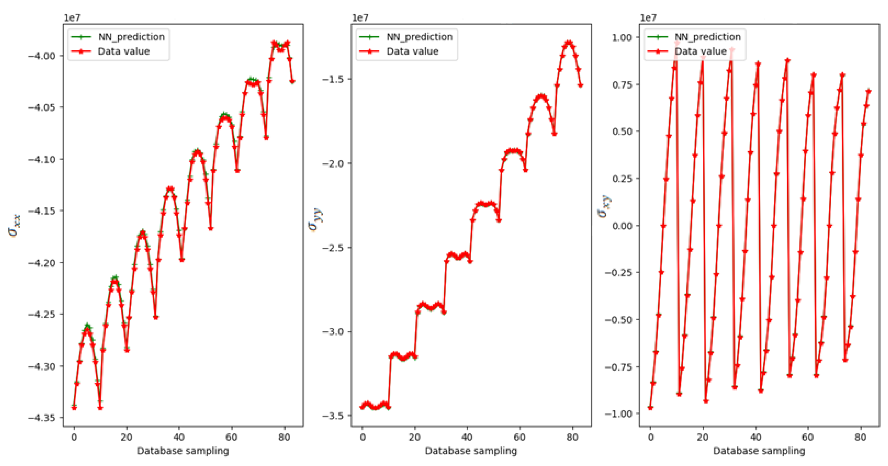
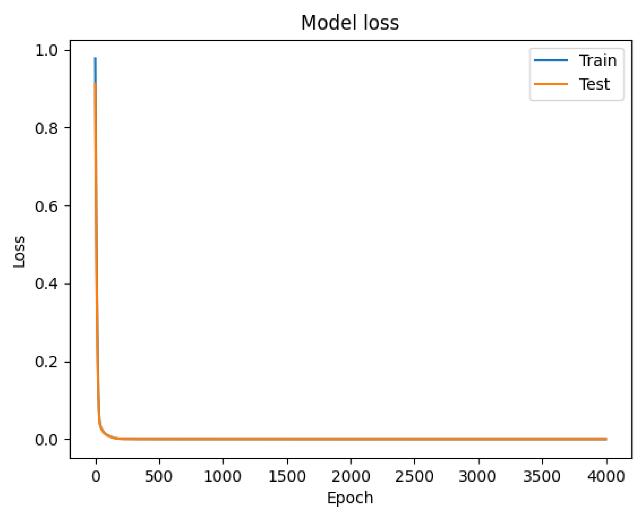
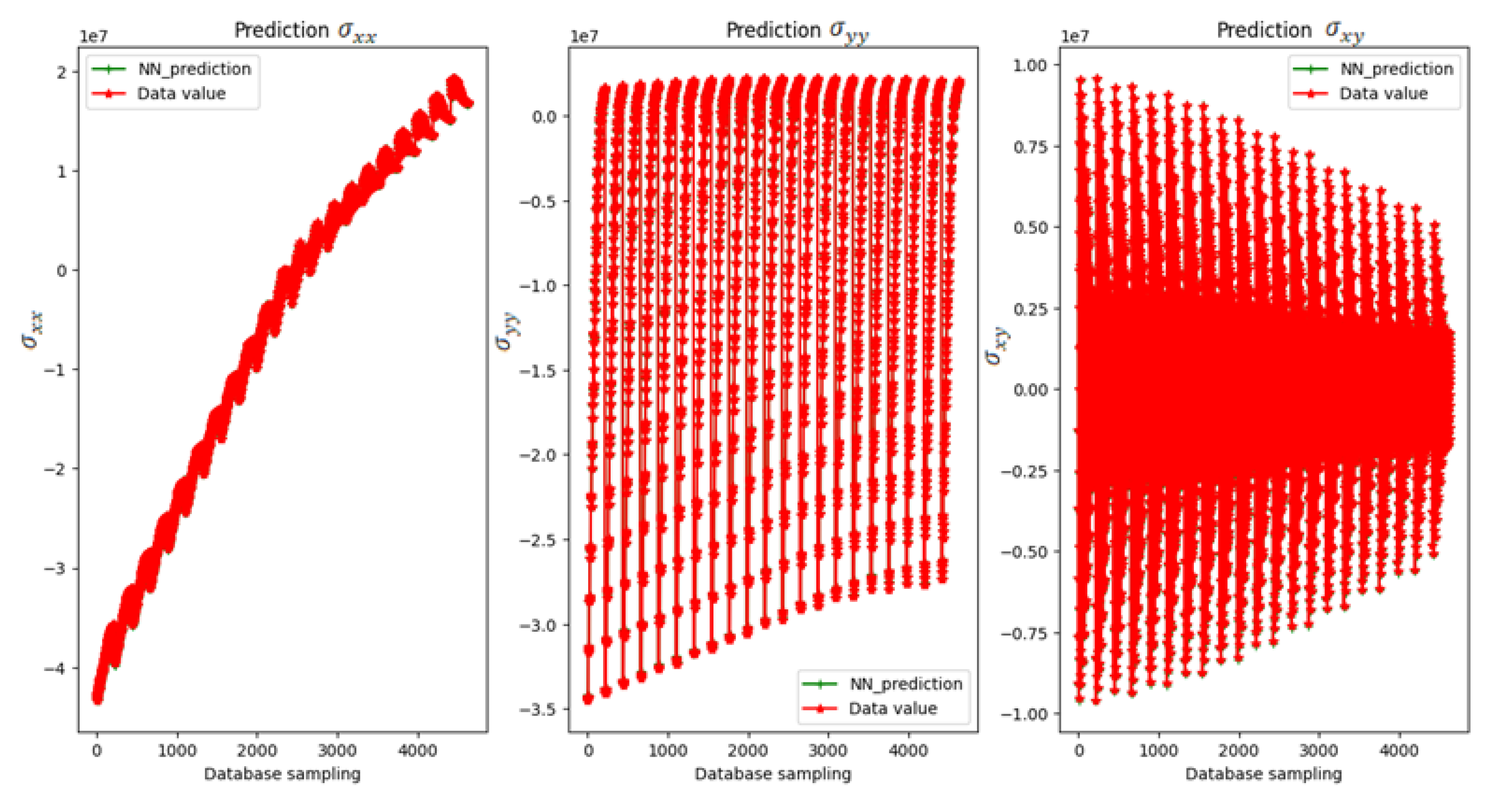
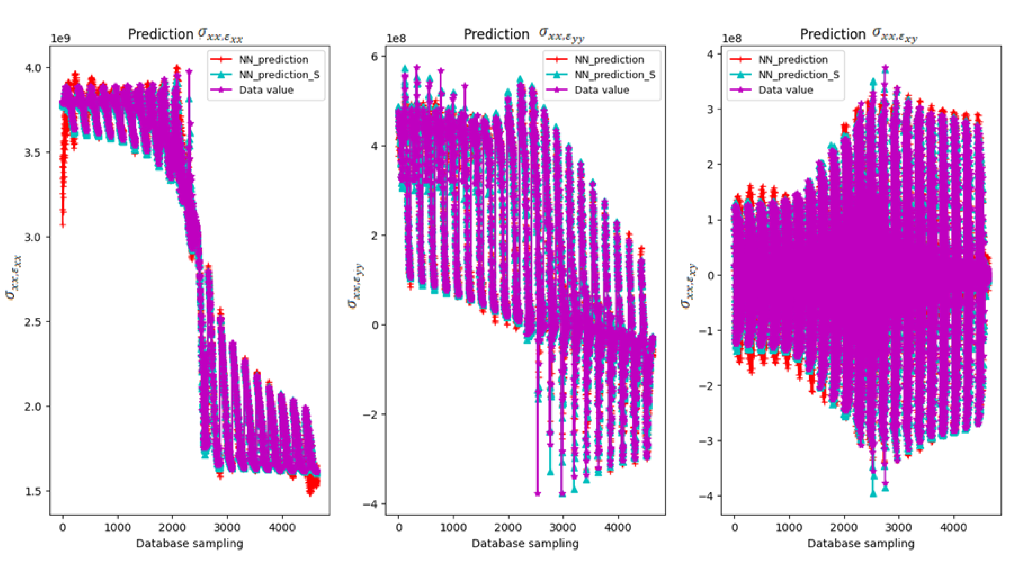
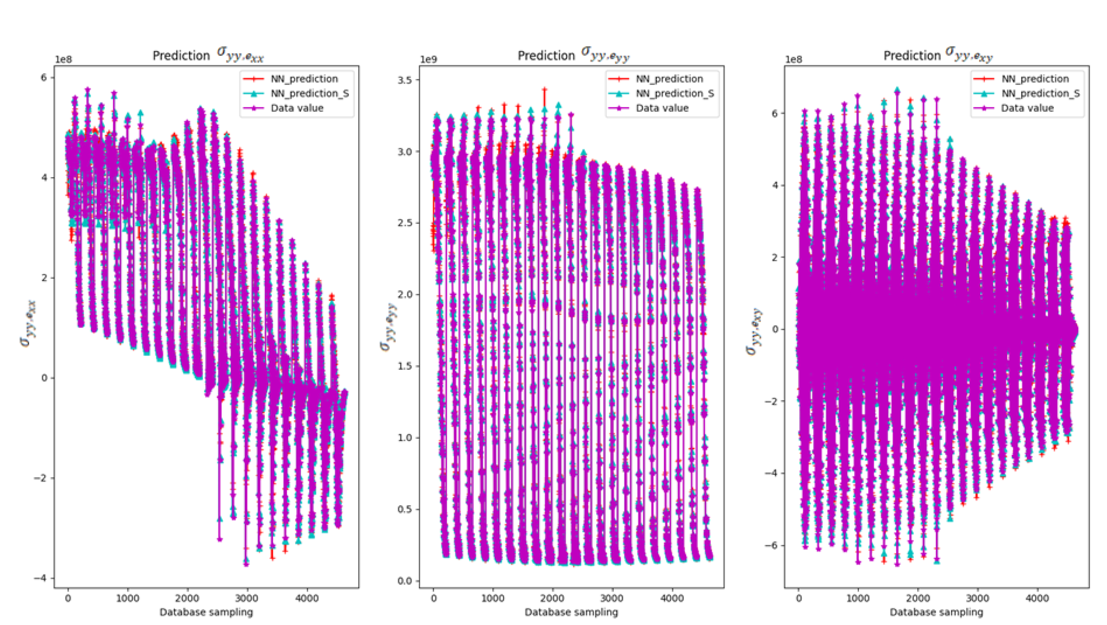
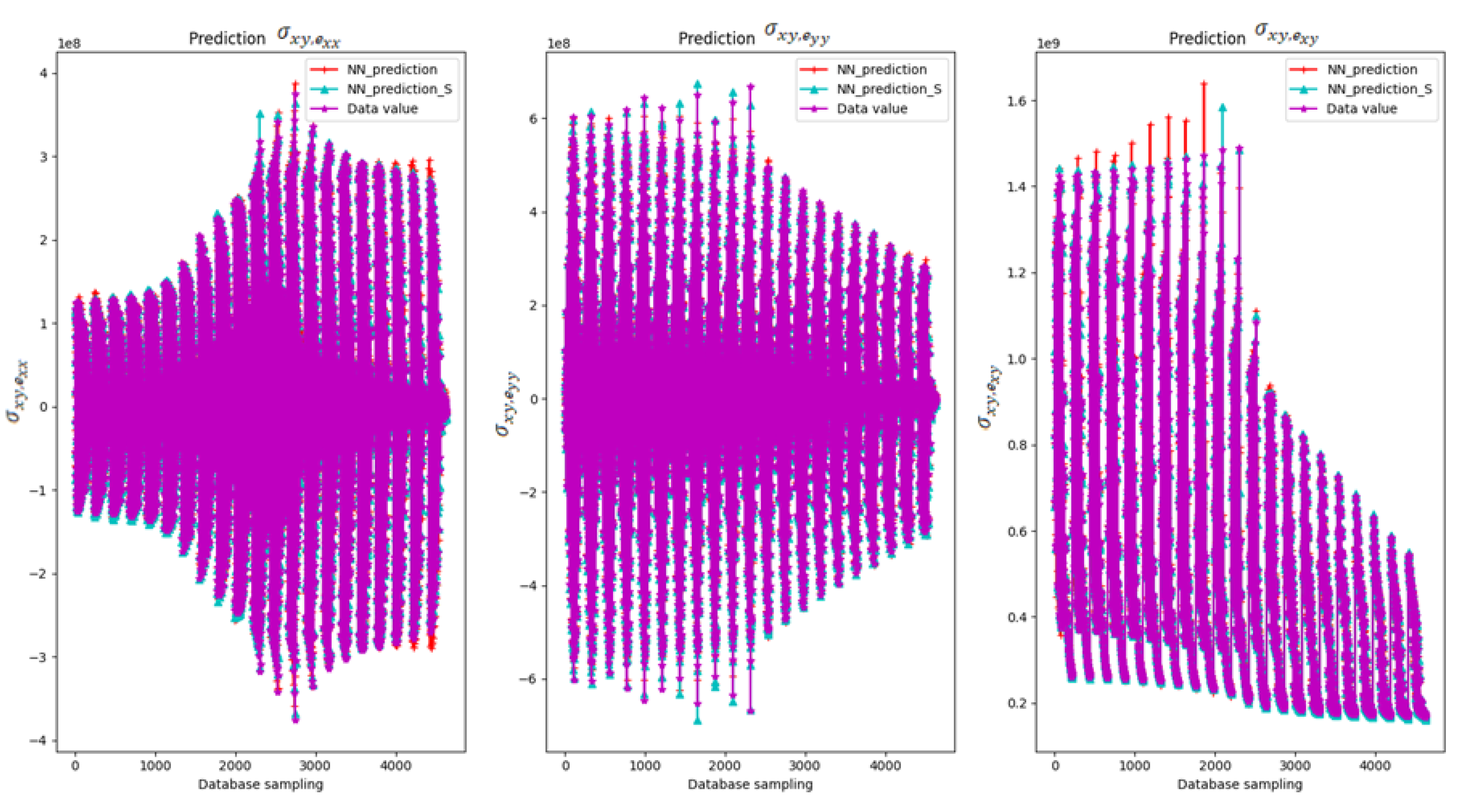
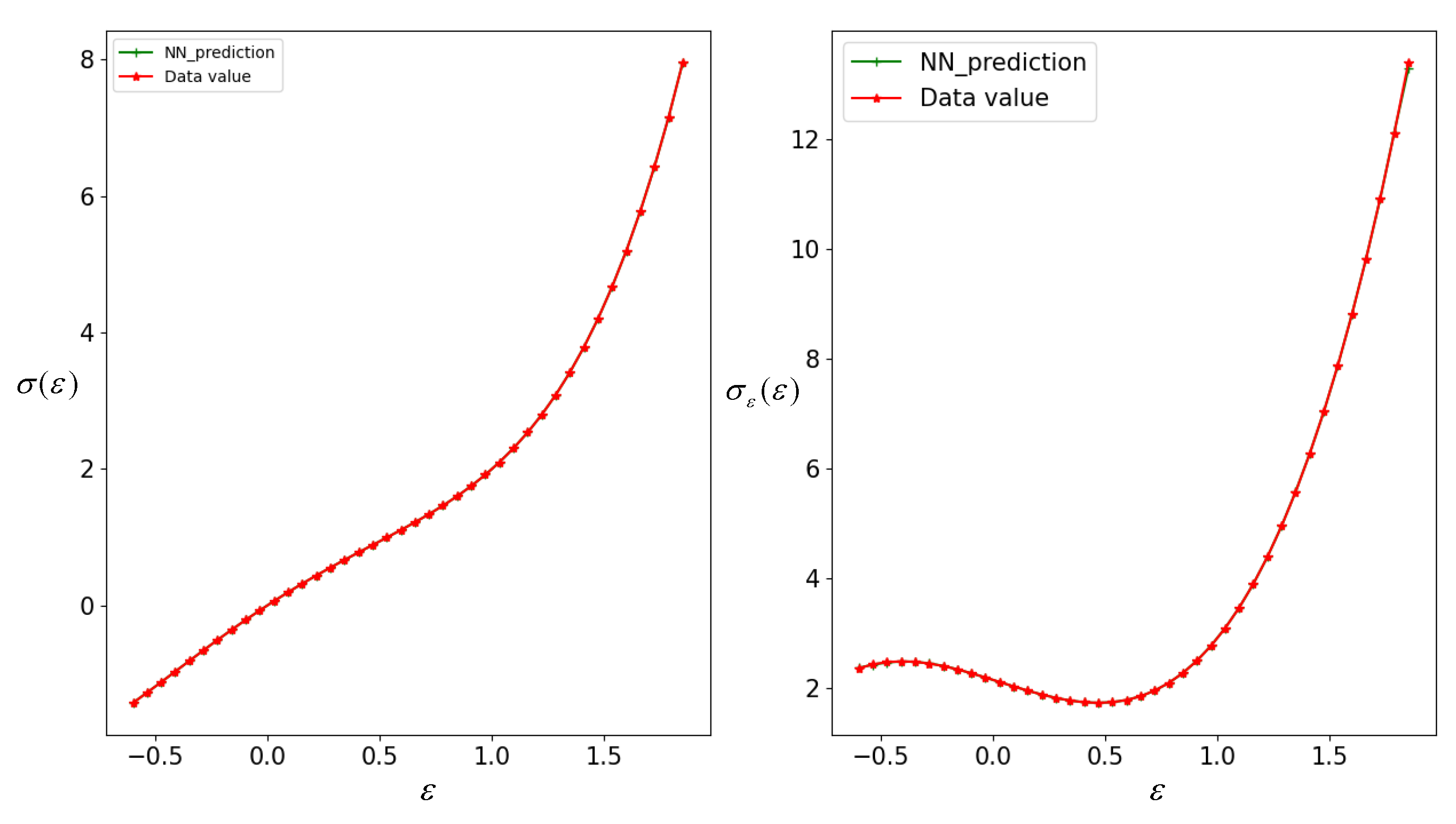
5. Numerical Results

Example 1.

The proposed neural constitutive network with the architecture presented in Figure 4 has been trained with different numbers of epochs, layers and neurons. The data for training and test with 9261 values for $\mathsf{\epsilon }$ and $\mathsf{\sigma }$ from the representative volume elements are considered. For the $\mathsf{\epsilon }$ we have

$$\begin{array}{ccc}\hfill {\epsilon }_{ij}^m& =& {\epsilon }_{ij}^{m-1}+h,h=0.001,\hfill \\ \hfill {\epsilon }_{ij}^1& =& -0.01,m=2,3,...M,M=21.\hfill \end{array}$$

(17)

In this example neural networks which consist from 4 hidden layers with [15, 20, 15, 20] neurons, respectively. The batch size is 64 and from the data-set $M=168$ values of the stress tensor (84 for the training and 84 for the test validation) are used to construct the neural constitute models with computations of the partial derivatives for the stress tensor. Batch size, which is an important key in machine learning and deep learning, refers to the number of training samples utilized in one iteration of model training. It can influence time of training, the efficiency and the model performance. The batch size can be chosen while training the model, e.g. in Keras library by the module "keras.models.Model.fit(xtrain, ytrain, validationdata= (xtest,ytest), epochs=nepochs, batchsize=64, verbose=2,callbacks=callbacks)".

Here, the formula (5) is used for the loss function, i.e. each surrogate model is trained separately. The results with 4000 training iterations are shown in Figure 6.

Figure 6 shows a match between data set and NN stress components. In Table 1 the error loss function

$$\mathrm{MSE}\sigma =max\{\mathrm{MSE}{\sigma }_{xx},\mathrm{MSE}{\sigma }_{yy},\mathrm{MSE}{\sigma }_{xy}\}$$

is given for different number of layers, neurons and epochs.

The time of computations can be decreased by using the three surrogate neural networks with the residual neural model, which include the residual (4), i.e. the loss error function includes all three components of the stress function. This approach is less expensive in sense of computation time and gives almost the same results. Figure 7 shows the loss function (4) while training the neural network to calculate the components of the stress tensor. The number of epochs is 4000. The neural network as before has 4 hidden layers with [15, 20, 15, 20] neurons, respectively. The batch size is 64 and from the data set we have taken the $M=82$ (42 for the training and 42 for the test validation) values of the stress tensor.

Example 2.

In this example the data set ($M=9261$) has been trained for getting a neural constitute model with computations of partial derivatives of the components of the stress tensor via the automatic differentiation. In Figure 8 the components of the stress tensor are presented and in Figure 9, Figure 10, Figure 11 the partial derivatives obtained from the components are sketched, respectively. The Sobolev error function (6) ($K=1$) is also used to train the neural network with the use of AD for the computation of the partial derivatives. Figure 9, Figure 10, and Figure 11 show that accuracy is better in the case of using the Sobolev metrics with the same number of training iterations. In this example, the neural network, which consists of 4 hidden layers with [15, 20, 15, 20] neurons with 5000 epochs, has been trained. The batch size is 64 and the data set has 9261 values for the components of the stress tensor (from which 4631 are used for the training and 4630 are used for the test validation). The test data are used for the comparison and validation of the results. In Table 2 the results of numerical experiments with different numbers of layers, neurons, and epochs are presented. It is noted that the accuracy of computations increase not only with increasing of number of epochs but also with increasing of number of layers and neurons.

The numerical experiments show that with larger number of epochs and hidden layers and neurons the results are more accurate. In case that derivative data are not available or Sobolev’s error is not included in the process, more training iterations are required in order to get a good accuracy for the derivatives.

From Figure 9, Figure 10, Figure 11 we can see the decreasing error after using the Sobolev metrics in the loss function of the training process. Thus, if the data for a stiffness matrix are available then the computations of the components of the stress tensor and its derivatives are more accurate.

Example 3.

In this example we consider uniaxial tension which is stretching along a single direction (or axis). It is the common and useful method for the mechanical testing of materials. The experiments have been done on hyperelastic materials with using polynomial model for nonlinear elastic deformations in polymers and rubbers (e.g., [44]). The stress-strain relation in tension can be written in a polynomial form for a nonlinear elastic material,

$$\sigma \left(\epsilon \right)=\sum _{i=1}^n=E_i{\epsilon }^i,$$

(18)

where $E_i$ are Young’s modulus. The case $E_2=E_3=E_4=0$ corresponds to Hook’s law from the linear elasticity theory. Tension has been tested for $E1=2.14663$ MPa, $E2=-0.646588$ MPa, $E3=-0.0697791$ MPa, $E4=0.566989$ MPa (Dastjerdi [44]).

In (17) we have taken ${\epsilon }_{ij}^1=-0.6,$$h=0.05$ and $N=50.$ The neural network has been trained with a data set, $M=90$ (45 for training and 45 for test validation) with 4 hidden layers and with [15,20,15,20] neurons, respectively. The number of epochs is 8000 and batch size is 64. The stress function with respect to the strain and its derivative are predicted on the data set $\{{\epsilon }_i,i=1,2,...,P\}$. The Sobolev training function is included in the loss function. The stress-strain curve and the derivative of the stress at the predicted points, $P=40$ with the exact values of the stress from the equation (18) are shown in Figure 12.

The loss error $MSE=5.7e-07$ and the relative errors of the computed stress values and its derivatives with respect to the strain at the predicted points are

$${\delta }_1={∥{\displaystyle \frac{{\sigma }^{\mathbf{NN}}-\sigma }{\sigma }}∥}_{\infty }=0.000424,{\delta }_2={∥{\displaystyle \frac{{\sigma }_{\epsilon }^{\mathbf{NN}}-{\sigma }_{\epsilon }}{{\sigma }_{\epsilon }}}∥}_{\infty }=0.008323.$$

Since the chain rule is used in the automatic differentiation the approximation of the derivatives can be done with a high accuracy. As the numerical results have been shown with even a small number of epochs we can get a good rate of convergences of the neural network to the data values if the stiffness matrix is included in training of the neural network.

6. Conclusions

A constitutive nonlinear neural network metamodel is proposed for calculating the constitutive relation in macrostructures. The components of the stress and strain tensor are used for training the neural network. The data set has been obtained after applying the representative volume elements. The neural network is constructed, based on the open scientific software machine learning platform Tensorflow and Keras library, written in Python. The values of components of stress tensor are predicted by the neural model and compared with the data set. The residual model is constructed with different loss function, including mean square error and the Sobolev function with the derivatives of the components of the stress tensor if the data for them are available. The latter gives better results after training the neural network. The proposed model allows to predict the stress tensor in macrostructures where the relations between stress and strain tensor are nonlinear. The proposed techniques can be applied to nonlinear structures and hyperelastic materials with large deflections. In these cases stress-strain relations have nonlinear behavior and can be simulated by the proposed here neural model, based on experimental or statistical data set in biological tissue (e.g aorta, blood vessels), elastomers, rubbers, polymers etc.

Extensions of this work in order to take into account path-dependent constitutive relation of the RVE and dynamic effects is possible on more complicated problems and constitute the subject of current research investigation.

References

1. Drosopoulos G., A. , Stavroulakis G. E., Non-linear Mechanics for Composite, Heterogeneous Structures, CRC Press, Taylor and Francis, 2022.
2. Urbański, A. , The unified, finite element formulation of homogenization of structural members with a periodic microstructure, Cracow University of Technology, 2005.
3. Geers, M.G.D. , Kouznetsova V. G., Brekelmans W.A.M., “Multi-scale computational homogenization: Trends and challenges”, J. Comput. Appl. Math. 2010, 234, 2175–2182. [Google Scholar]
4. Kortesis, S. and Panagiotopoulos P. D., Neural networks for computing in structural analysis: Methods and prospects of applications, Int. J. for Num. Meth. in Eng. 1993, 36, 2305–2318. [Google Scholar]
5. Avdelas, A.V. , Panagiotopoulos P. D. , Kortesis S., Neural networks for computing in the elastoplastic analysis of structures, Meccanica 1995, 30, 1–15. [Google Scholar]
6. Stavroulakis G., E. , Avdelas A., Abdalla K. M., Panagiotopoulos P. D. A neural network approach to the modelling, calculation and identification of semi-rigid connections in steel structures, J. of Constructional Steel Research 1997, 44(1–2), 91-105.
7. Stavroulakis, G. , Bolzon G, Waszczyszyn Z. and Ziemianski L. Inverse analysis. In: Karihaloo B, Ritchie RO, Milne I (eds in chief) Comprehensive structural integrity, Numerical and computational methods 2003, 3, Chap–13, Elsevier,Amsterdam,685–718. [Google Scholar]
8. Stavroulakis G., E. Inverse and identification problems in mechanics. Springer / Kluwer Academic 2000.
9. Waszczyszyn, Z. and Ziemiański L., Neural Networks in the Identification Analysis of Structural Mechanics Problems. In: Mróz Z., Stavroulakis G.E. (eds), Parameter Identification of Materials and Structures, CISM International Centre for Mechanical Sciences (Courses and Lectures), 2005; 469, Springer, Vienna.
10. Muradova A., D. , Stavroulakis G. E., The projective-iterative method and neural network estimation for buckling of elastic plates in nonlinear theory, Comm. in Nonlin. Sci. and Num. Sim. 2007, 12, 1068–1088. [Google Scholar]
11. Yagawa G, Oishi A. Computational mechanics with neural networks, Springer, 2021.
12. Dornheim, J. , Morand L. , Nallani H. J., Helm D., Neural Networks for Constitutive Modeling: From Universal Function Approximators to Advanced Models and the Integration of Physics, Arch. of Comp. Meth. in Eng. 2024, 31, 1097–1127. [Google Scholar] [CrossRef]
13. Linka, K. , Hillgärtner M. , Abdolazizi K. P., Aydin R. C., Itskov M., Cyron Ch. J. Constitutive artificial neural networks: A fast and general approach to predictive data-driven constitutive modeling by deep learning, Journal of Computational Physics 2021, 429, 110010. [Google Scholar]
14. Linka, K. , Kuhl E. , A new family of Constitutive Artificial Neural Networks towards automated model discovery, Comput. Methods Appl. Mech. Engrg. 2023, 403, 115731. [Google Scholar]
15. Haghighat, E. , and Juanes, R. Sciann, A keras/tensorflow wrapper for scientific computations and physics-informed deep learning using artificial neural networks, Comput. Meth. in Appl. Mech.s and Eng. 2021, 373, 113552. [Google Scholar]
16. Baydin, A. , Pearlmutter B. A., Radul A. A., Siskind J. M., “Automatic Differentiation in Machine Learning: a Survey”, 2018, https://arxiv.org/pdf/1502.05767.pdf.
17. Czarnecki W., M. , Osindero S., Swirszcz M. J. G., and Pascanu R., “Sobolev Training for Neural Networks”, https://arxiv.org/pdf/1706.04859.
18. Michel J-C. , Moulinec H., Suquet P., Effective properties of composite materials with periodic microstructure: a computational approach, Comput. Meth. Appl. Mech. Eng. 1999, 172, 109–143.
19. Zohdi, T.I. , Wriggers P., An introduction to computational micromechanics. Springer, Berlin, 2008.
20. Tikarrouchine, E. , Benaarbia A. , Chatzigeorgiou G., Meraghni F., Non-linear FE2 multiscale simulation of damage, micro and macroscopic strains in polyamide 66-woven composite structures: Analysis and experimental validation, Composite Structures 2021, 255, 112926. [Google Scholar]
21. Drosopoulos G., A. , Giannis K., Stavroulaki M.E., Stavroulakis G. E., Metamodeling-assisted numerical homogenization for masonry and cracked structures, ASCE Jr. of Eng. Mech. 2018, 144(8), art. no. 04018072.
22. Drosopoulos G., A. , Stavroulakis G. E., Data-driven Computational Homogenization Using Neural Networks: FE2-NN Application on Damaged Masonry, ACM Jr. on Comp. and Cultural Heritage 2020, 14(1), 1-19.
23. Yvonnet, J. , He Q. C., Li P., Reducing internal variables and improving efficiency in data-driven modelling of anisotropic damage from RVE simulations, Comput. Mech. 2023, 72, 37–55. [Google Scholar]
24. Le, B.A. , Yvonnet J. , He Q.-C. , Computational homogenization of nonlinear elastic materials using neural networks, Int. J. for Num. Meth. in Eng. 2015, 104(12), 1061–1084. [Google Scholar]
25. Urbański, A. , Szymon l. , Marcin D., Multi-scale modeling of brick masonry using a numerical homogenization technique and an artificial neural network, Arch. of Civil Eng. 2022, 68(4), 179–197. [Google Scholar]
26. Eivazi H., Tröger J.-A., Wittek S., Hartmann S., Rausch A., “FE2 Computations With Deep Neural Networks: Algorithmic Structure, Data Generation, and Implementation” (June 07, 2023). Available at SSRN: https://ssrn.com/abstract=4485434 or http://dx.doi.org/10.2139/ssrn.4485434. [CrossRef]
27. Fish, J. , Yu Y. , Data-physics driven reduced order homogenization, Int. J. Numer. Methods Engrg. 2023, 124(7), 1620–1645. [Google Scholar] [CrossRef]
28. As’ ad, F. , Avery P. , Farhat C., A mechanics-informed artificial neural network approach in data-driven constitutive modeling, Int. J. Numer. Methods Engrg. 2022, 123(12), 2738–2759. [Google Scholar]
29. Protopapadakis, E. , Schauer, M. , Pierri, E., Doulamis, A. D., Stavroulakis, G. E., Böhrnsen, J.-U., Langer, S., A genetically optimized neural classifier applied to numerical pile integrity tests considering concrete piles, Computers and Structures 2016, 162, 68–79. [Google Scholar]
30. Muradova A.D., Stavroulakis G.E., Physics-informed neural networks for elastic plate problems with bending and Winkler-type contact effects, J. of the Serbian Society for Comput. Mech. 2021, 15(2), 45-54.
31. Mouratidou A., D. , Drosopoulos G. A., Stavroulakis G. Ensemble of physics-informed neural networks for solving plane elasticity problems with examples, Acta Mechanica, 2024. [Google Scholar] [CrossRef]
32. Karniadakis, G.E. , Kevrekidis I. G., Lu L. et al., “Physics-informed machine learning”, Nat. Rev. Phys. 2021, 3, 422–440. [Google Scholar] [CrossRef]
33. Katsikis, D. , Muradova A. D. and Stavroulakis G. S., A Gentle Introduction to Physics-Informed Neural Networks, with Applications in Static Rod and Beam Problems, J. of Adv. in Appl. & Comput. Math. 2022, 9, 103–128. [Google Scholar]
34. Lu, X. , Giovanis D.G., Yvonnet J., Papadopoulos V., Detrez F., Bai J., A data-driven computational homogenization method based on neural networks for the nonlinear anisotropic electrical response of graphene/polymer nanocomposites, Comput. Mech. 2019, 64(2), 307-321.
35. Fish, J. , Wagner G.J., Keten S., Mesoscopic and multiscale modelling in materials. Nat. Mater. 2021, 20, 774–786. [Google Scholar] [CrossRef] [PubMed]
36. Tchalla, A. , Belouettar S. , Makradi A., Zahrouni H., An ABAQUS toolbox for multiscale finite element computation, Composites Part B: Engineering 2013, 52, 323–333. [Google Scholar]
37. Wei H., Wu C.T., Hu W. et al., LS-DYNA Machine Learning–Based Multiscale Method for Nonlinear Modeling of Short Fiber–Reinforced Composites, J. of Eng. Mech. 2023, 149(3).
38. Tung-Huan Su and others, Multiscale computational solid mechanics: data and machine learning, J. of Mech. 2022, 38, 568–585.
39. Fei, T. , Xin L. , Haodong D., Wenbin Y., Learning composite constitutive laws via coupling Abaqus and deep neural network, Composite Structures 2021, 272, 114137. [Google Scholar]
40. Stavroulakis G., E. , Konstadinos G., Drosopoulos G. A., Stavroulaki M. E., Non-linear Computational Homogenization Experiments, Proc. COMSOL Conference 2013 Rotterdam: https://www.comsol.de/paper/download/182535/stavroulakis- paper.pdf.
41. Barron A. R., Approximation and Estimation Bounds for Artificial Neural Networks, Machine Learning 1994, 14, 115-133.
42. Ruder, S. An overview of gradient descent optimization algorithms 2017,https://arxiv.org/abs/1609.04747.
43. Abadi, M. , Barham P., Chen J., Chen Z., Davis A., Dean J., Devin M., Ghemawat S., Irving G., Isard M., Kudlur M., Levenberg J., Monga R., Moore S., Murray D.G., Steiner B., Tucker P., Vasudevan V., Warden P., Wicke M., Yu Y., Zheng X., Tensorflow: A system for large-scale machine learning, in: 12th USENIX Symposium on Operating Systems Design and Implementation (OSDI 16), USENIX, Association, Savannah, GA, 2016, 265–283, URL https://www.usenix.org/conference/osdi16/technical-sessions/presentation/abadi.
44. Dastjerdi, S. , Alibakhshi A., Akgöz B., Civalek O., Novel Nonlinear Elasticity Approach for Analysis of Nonlinear and Hyperelastic Structures, Engineering Analysis with Boundary Elements, 2022, 143, 219-236.
1
The programming code is available from the supplemental material as an open source.
Figure 1. The concept of FEM multi-scale modeling.
Preprints 147068 g001
Figure 2. Replacing the σ ε constitutive relation of the RVE by an artificial neural network.
Preprints 147068 g002
Figure 3. Plastic deformation of the masonry RVE.
Preprints 147068 g003
Figure 4. The architecture of the neural constitutive model ε σ , σ / ε with training data ( ε data , σ data ) and the mean square error (MSE).
Preprints 147068 g004
Figure 5. The flowchart for the neural network model used to predict components of the stress tensor based on the data-set from the representative volume elements.
Preprints 147068 g005
Figure 6. The components of the stress tensor after training of the neural network (Figure 4) and the data-set ( M = 82 ), obtained from the representative volume elements.
Preprints 147068 g006
Figure 7. The dynamics of the model loss function (4) while training the network with three surrogate neural models and one residual model for computing the components of the stress tensor.
Preprints 147068 g007
Figure 8. The components of the stress tensor after training of the neural network (Figure 4) and from the data-set ( M = 9261 ), obtained from the representative volume elements.
Preprints 147068 g008
Figure 9. The partial derivatives of the components of the stress tensor σ x x after training of the neural network (Figure 4) and from the data set M = 9261 , obtained from representative volume elements.
Preprints 147068 g009
Figure 10. The partial derivatives of the components of the stress tensor σ y y after training of the neural network Figure 4 and from the data set M = 9261 , obtained from representative volume elements.
Preprints 147068 g010
Figure 11. The partial derivatives of the components of the stress tensor σ x y after training of the neural network Figure 4 and from the data set M = 9261 , obtained from representative volume elements.
Preprints 147068 g011
Figure 12. The stress-strain curve and the derivative function of stress of the hyperelastic material from the prediction of the neural network and from the data values.
Preprints 147068 g012