
Submitted:
07 November 2025
Posted:
10 November 2025
You are already at the latest version
Abstract
Due to the increasing concern over climate change and its environmental impacts, effective greenhouse gases (GHG) control strategies are of pivotal importance. The use of models such as STILT (Stochastic Time Inverted Lagrangian Transport), statistical techniques, and experimental data analysis provide valuable tools to quantify emissions and identify GHG tendencies. The Mediterranean basin is considered a global hotspot for air-quality and climate change: here, we combine experimental datasets of atmospheric methane (CH4) and carbon dioxide (CO2) with atmospheric transport models to present an atmospherically-based framework for monitoring GHG emissions. We applied methodologies, i.e., the Smoothed Minima (SM) and STILT, to extract background concentration data from the time series of atmospheric gases and identify measurements deemed representative of atmospheric background (GRD) levels. At the Lamezia Terme (Global Atmosphere Watch, GAW code: LMT), Capo Granitola (GAW code: CGR), and Lampedusa (GAW code: LMP) observation sites, GHG measurements were performed with specific calibration routines carried out using primary standards of calibration from the National Oceanic and Atmospheric Administration – Global Monitoring Laboratory (NOAA–GML), with secondary standards used to evaluate possible drifts and calibration factors stability. The first two are coastal stations and the third is an island station. At these sites, atmospheric CH4 and CO2 mole fractions can be evaluated at local and continental scales, in locations with specific Mediterranean climatic characteristics. This paper presents the variability of CH4 and CO2 in the central Mediterranean basin by analyzing hourly GHG concentrations over a 9-year period (2015-2023) for LMT, a 8-year period (2015-2022) for CGR, and a 19-year period (2006-2024) for CO2 and 5-year period (2020-2024) for CH4 at LMP. STILT provides 3-hourly results for methane and carbon dioxide concentrations that correlate well with surface measurements at LMT, CGR, and LMP. These analyses are aimed at relevant long-term datasets of GHG over southern Italy. This work would provide a useful contribution to comparing the observed concentrations of gases measured at three sites in the central Mediterranean with those predicted by models such as STILT.
Keywords:
STILT
; GAW
; Southern Italy
; greenhouse gas
; methane
; carbon dioxide
; emissions
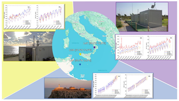
Graphical abstract descriptions
Framework shows the variability of methane and carbon dioxide in the Mediterranean basin at three permanent World Meteorological Organization/Global Atmosphere Watch (WMO/GAW) stations in southern Italy: Lamezia Terme (GAW code: LMT), Capo Granitola (GAW code: CGR) and Lampedusa (GAW code: LMP). Accurate modeling of atmospheric transport is essential to address environmental concerns and to establish a quantitative link between observed gas distributions and surface emissions. In the present work, we used the Stochastic Time Inverted Lagrangian Transport (STILT) and the Smoothed Minima (SM) models. STILT simulates transport by following the time evolution of a particle ensemble, interpolating meteorological fields to the subgrid location of each particle. Both methods were used to extract background concentration data from the time series of atmospheric gases representative of the atmospheric background levels. The paper is an important contribution to the comparison between the observed and predicted by models concentrations of methane and carbon dioxide at three sites in the central Mediterranean. The STILT model datasets, validated at the three sites, show satisfactory results, with the exception of an overall underestimation in all comparisons (background and no-background). They demonstrate that the model can accurately estimate the CH4 and CO2 concentrations in the Mediterranean basin. Similar results are also obtained when comparing the SM and STILT background datasets. This last comparison indicates a good identification of the concentrations of the background gases by the models.
1. Introduction
Southern Europe and the Mediterranean basin are recognized as hotspots in terms of both air quality (Monks et al., 2009) and climate change (Giorgi and Lionello, 2008), as well as a major intersection of different air mass transport processes (Lelieveld et al., 2002; Henne et al., 2004; Duncan et al., 2008). The Fourth Assessment Report of the Intergovernmental Panel on Climate Change (IPCC, 2007) clearly identifies and assesses the rising levels of greenhouse gases (GHG) in global warming (Forster et al., 2007). Furthermore, the IPCC's Sixth Assessment Report (AR6) is an extensive analysis of the latest climate science, its impacts, and mitigation strategies. It is the culmination of the IPCC's work. This work was done during its sixth assessment cycle. AR6 provides in-depth assessments of the physical science basis of climate change, its impacts, adaptation strategies, and mitigation options. The report highlights progress in mitigating climate change, including the slowing growth rate of global greenhouse gas emissions in recent years and the rapid development of low-carbon electricity generation and storage technologies. However, it also acknowledges ongoing challenges. It also brings attention to the Sustainable Development Goals. Climate action is critical to sustainable development. The report analyzes the relationship between greenhouse gas (GHG) emissions per capita and development levels to establish sustainable development pathways and corridors (IPCC, 2023). The role played by the Mediterranean in the global carbon dioxide (CO2) budget is poorly detailed. In fact, the Mediterranean Sea has several peculiarities that make it unique: it is the only large closed basin in the world and is characterized by complex oceanic and atmospheric circulation (Chamard et al., 2003). To better understand the role of the Mediterranean Sea, accurate long-term measurements of atmospheric gas concentrations are essential, especially in the coastal and marine environments. Ever since 1750, the date universally recognized as the beginning of the Industrial Revolution, a rapid increase in carbon dioxide has been observed, and present-day levels are still on the rise (Friedlingstein et al., 2023). In order to define the global atmospheric gas budget and constrain its sources and sinks, accurate long-term measurements of atmospheric concentrations began about 50 years ago at Mauna Loa (Hawaii, USA) (Keeling et al., 1976; Keeling, 2008). The Global Atmosphere Watch (GAW) program, established by the World Meteorological Organization (WMO) (World Meteorological Organization Global Atmosphere Watch No. 168, 2005), has developed a globally distributed network of GHG monitoring stations. Current CO2 observations are still lacking in some areas of the globe. Focusing on the Mediterranean basin, the Lamezia Terme (mainland Calabria) and Capo Granitola (mainland Sicily) coastal sites, and the Lampedusa (Strait of Sicily) maritime site all perform continuous measurements of GHG. The CNR-ISAC (National Research Council of Italy – Institute of Atmospheric Sciences and Climate) observatory in Lamezia Terme (GAW code: LMT, 38.8°N 16.2°E, 6 meters above sea level) is a Regional WMO/GAW station; atmospheric concentrations of methane (CH4), carbon dioxide and other gases are routinely measured since 2015. The GAW Regional Coastal Observatory of Capo Granitola (GAW code: CGR, 37.6°N 12.6°E, 5 meters above sea level) faces the Strait of Sicily in the coastal area of Torretta Granitola, 12 km from Mazara del Vallo (province of Trapani). The Strait of Sicily is characterized by heavy shipping traffic, making the central Mediterranean a European hotspot for the impact of ship emissions on air chemistry (EEA 2013). CGR is a remote site influenced by anthropogenic emissions related to shipping operations at the port of Mazzara, located about 20 kilometers away. A long-term GHG monitoring programme has been initiated by ENEA (the Italian National Agency for New Technologies, Energy and Environment) in May 1992, for background CO2 measurements at the remote island of Lampedusa (GAW code: LMP, 33.5°N 12.6°E) (Chamard et al., 2003; Artuso et al., 2009). Lampedusa is currently the only dual GAW and National Oceanic and Atmospheric Administration (NOAA) maritime site for CO2 observations in the Mediterranean. The island was chosen because of its geographical position, which makes it particularly suitable for climate studies. NOAA established a global measurement network of CO2 and other climate-relevant gases in the late 1970s (Conway et al., 1994; Tans et al., 1989). On a global scale, CH4 and CO2 records are used to understand the processes that govern the gases cycle, which are essential for predicting its future tendencies and planning international policy strategies to reduce them. The long-term behavior of CO2 is a combination of a gradual increase in emissions, overlaid by a large inter-annual variability associated with climate-driven changes in the strength of sources and sinks (Rayner and Law, 1999; Keeling et al., 1995). Carbon isotope measurements of CO2 (δ13CO2) confirm that the increases are attributable to fossil fuel burning: during the summer, the peak in plant photosynthesis results into the highest δ13CO2 values and the lowest CO2 atmospheric concentrations of the year due to the isotopic fractionation that occurs during the photosynthesis process, which fractionates against the heavier 13CO2 isotopologue of carbon dioxide, thus increasing its residual concentration in the atmosphere (Farquhar et al., 1980; Farquhar et al., 1989). The atmospheric pattern is compatible with the isotopic fingerprint of fossil fuels as the wintertime tendencies are reversed: higher CO2 concentrations are linked to lower δ13CO2 values due to anthropogenic emissions (Keeling et al., 1979; Keeling, 1979). Human activities have contributed to a significant increase in atmospheric of CH4 and CO2. Changes in land use are causing a significant reduction in the CO2 uptake capacity of plants, reinforcing the general global upward tendency (Canadell et al., 2007). Saharan dust outbreaks from North Africa (Querol et al., 2009) and widespread open burning of biomass (Turquety et al., 2014) further exacerbate air quality and the impact of anthropogenic emissions on the regional climate (Mallet et al., 2013). Information on the variability of gases in the atmosphere is provided by experimental measurements on a continental scale. CH4 plays an important role in the Earth's atmospheric chemistry and radiation balance: it is the most abundant hydrocarbon in the atmosphere, and after CO2, is the second most relevant GHG. Methane’s persistence time in the atmosphere is lower compared to that of carbon dioxide, but its global warming potential is higher (Myhre et al., 2013; Sand et al., 2023). In the stratosphere and troposphere, methane reacts with the hydroxyl radical OH, which is its primary sink, to produce water vapor and ultimately CO2, indirectly contributing to the build-up of atmospheric CO2 (Artuso et al., 2007). Methane has also been on the rise ever since the industrial period, an increase that is linked to anthropogenic activities (Etheridge et al., 1998). Unlike CO2 however, the global carbon isotope patterns observed in CH4 (δ13CH4) indicate that perturbations in the global budget caused by anthropogenic emissions are not sufficient to explain atmospheric methane increases, as changes in natural emissions and balances in said budget also have an impact on recent tendencies (Ferretti et al., 2005; Nisbet et al., 2019). Furthermore, unlike other gases and pollutants, methane experienced a rise during COVID-19 lockdowns due to increased emissions from domestic heating and changes in atmospheric sinks; this increase has been observed at a global scale (Laughner et al., 2021; Peng et al., 2022), and at local scale in the case of the LMT observatory (D’Amico et al., 2024a; D’Amico et al., 2024c). The importance of greenhouse gases is well known and has been described in literature (Seinfeld and Pandis, 1998): the utilization of models for the purpose of providing support and facilitating the integration of experimental data is advantageous. There are different types of models, some of which focus on vehicles as local sources (Batesa et al., 2018), and these methods can be extended to other local non-road facilities. Generally, the inclusion of comprehensive local and regional sources and chemistry with fine-scale spatial gradients can provide comprehensive estimates of pollutant concentrations, reducing bias in exposure estimates used for epidemiological analyses. Results are currently being used in spatiotemporal epidemiological analyses of birth outcomes associated with air pollution, and in urban planning and environmental law studies investigating the relationships between infrastructure characteristics, socio-economic factors, health, and air pollution (Batesa et al., 2018; Servadio et al., 2019). Models exist to determine background concentrations of atmospheric gases (Malacaria et al., 2025). In this work, we have applied a Lagrangian Particle Dispersion Model (LPDM) for atmospheric transport, the Stochastic Time-Inverted Lagrangian Transport model (STILT), as well as the Smoothed Minima (SM) (Malacaria et al., 2025; Aksoy et al., 2009; Gao et al., 2018) background methods to the experimental datasets of CH4 and CO2 concentrations at the LMT, CGR, and LMP stations. STILT is used to derive the upstream influence on atmospheric sites, i.e., their footprint. These footprints are combined with surface maps of natural and anthropogenic tracer fluxes to simulate atmospheric tracer concentrations at the analyzed stations. The particles in this model are tracked back up to 10 days. A novelty is the implementation of GHG measurements at tower sites to complement atmospheric monitoring from free tropospheric sites, aircraft, and high towers: a southern Italian station (Potenza) located in the southern Italian region of Basilicata, is expected to start such measurements soon, further contributing to data gathering in the central Mediterranean region. This provides a strong link between observations at continental and ecological scales. An important step towards an operational European greenhouse gas-monitoring program has now been taken with the proposal for an Integrated Carbon Observation System (ICOS). This project aims to establish an integrated European greenhouse gas-monitoring network, incorporating existing monitoring stations and extending the network to areas not covered by operating stations. Such an integrated European monitoring program appears to be essential to ensure the availability of long-term, high-precision measurements of atmospheric greenhouse gases. With the planned ≈30 operational 'backbone' European atmospheric monitoring sites, the ICOS network would provide a solid basis for top-down estimates of European greenhouse gas emissions. In addition to an adequate European network, it would be important to support further global observing stations, especially in regions with large emissions or tendencies (i.e., China, India), and satellite retrievals, especially for CH4 and CO2, for which recent research has shown significant progress and the potential to provide valuable complementary information in regions with scarce in situ monitoring (i.e., tropical landmasses). In the following sections, the measurement sites are presented in terms of the experimental set-up. We present 9 (8) years of precise measurements of CH4 and CO2 at LMT (CGR), plus 19 years of CO2 and 5 years of CH4 both detected at LMP. Typical concentrations and variability of CH4 and CO2 in the central Mediterranean are the subject of analysis and discussion: we compare the experimental datasets of these stations with STILT and SM models in order to evaluate possible mechanisms influencing the Mediterranean carbon budget, some of which could be overlooked by models.
2. Description of the Experimental Sites
The Lamezia Terme, Capo Granitola, and Lampedusa Experimental Sites
The Lamezia Terme (GAW ID: LMT, 38.8°N 16.2°E, 6 meters above sea level) station is a World Meteorological Organization/Global Atmosphere Watch (WMO/GAW) observatory operated by the National Research Council of Italy - Institute of Atmospheric Sciences and Climate (CNR-ISAC) ever since 2015. LMT is a coastal site located 600 meters inland from the Tyrrhenian coastline of Calabria (Southern Italy) (Figure 1). Here the dominant air masses of the synoptic circulation overlap with the local breezes, maintaining a strong westerly direction. The experimental site is characterized by moderate daytime seaside breezes (NW-W), while night-time northeastern breezes from the land (E-SE) are channeled through the Marcellinara gap, located between the Tyrrhenian and Ionian Seas (Calidonna et al., 2020; Malacaria et al., 2024; Federico et al., 2010a; Federico et al., 2010b; D’Amico et al., 2024a; D’Amico et al., 2024d). Local wind circulation has been confirmed to have a relevant influence on LMT observations, with western-seaside winds generally yielding low concentrations of GHGs and pollutants, while northeastern-continental winds are enriched in these compounds (D’Amico et al., 2024a; D’Amico et al., 2024c). Surface ozone (O3) at the site however was confirmed to have a reversed pattern (D’Amico et al., 2024d). Peplospheric fluctuations and changes in wind regimes also affect the surface concentrations of parameters observed at LMT, further contributing to the complexity of correlations between wind patterns and the concentrations of GHG and pollutants (D’Amico et al., 2024e).
The Capo Granitola Observatory (GAW ID: CGR, 37.6°N 12.6°E, 5 meters above sea level) is located on the southern coast of Sicily, facing the Strait of Sicily, at Torretta Granitola, 12 km from Mazara del Vallo (52,000 inhabitants), within the scientific campus of CNR’s Institute for the study of anthropogenic impacts and sustainability in the marine environment (IAS). CGR is a remote site and it is an ideal station for monitoring marine background conditions, https://gawsis.meteoswiss.ch/GAWSIS//index.html#/search/station/stationReportDetails/0-20008-0-CGR (accessed on November 2024).
This observatory carries out continuous measurements of atmospheric composition that are well representative of the conditions in Western Sicily and the central Mediterranean basin: it often observes air masses that are characteristic of the background conditions in the Mediterranean basin. These air masses provide useful clues to the influence of specific atmospheric processes when strong tracer variability is encountered. Mineral dust emitted from North Africa, long-range air mass transport, and anthropogenic ship-borne emissions could be some of these processes. The CGR site is influenced by the sea-land breeze regime, with prevailing winds of up to 4 m/s, gentle breezes from inland (NW-NE) during the night and prevailing winds from the sea (W-SE) during the day (Cristofanelli et al., 2017; Donateo et al., 2018; Donateo et al., 2020). CGR is strongly influenced by air masses originating or passing over the central Mediterranean (Tyrrhenian Sea), which have a prevailing northwesterly circulation (Cristofanelli et al., 2017).
Lampedusa (GAW ID: LMP, 33.5°N 12.6°E) is a small island in the Mediterranean sea, approximately 250 km south of Sicily and 130 km east of Tunisia. The island, whose position is shown in Figure 1, is isolated in the marine environment, about 200 km from northern Libya. The island covers an area of 20 km2, and shows sparse and rocky vegetation. The influence of local vegetation and emissions is expected to be limited. As a representative site for the central Mediterranean region, the island was chosen for greenhouse gas measurements in early 1990’s (Chamard et al., 2003). Air samples are collected from about 8 m above the surface, on a promontory on the north-eastern edge of Lampedusa (50 m above sea level). The site is operated by ENEA, the Italian National Agency for New Technologies, Energy and Sustainable Economic Development.
3. Data and Methods
3.1. Instrumental Set-Up and Sampling Systems
At LMT and CGR a CRDS (Cavity Ring-Down Spectroscopy) analyzer (Picarro model G2401, Santa Clara, California, USA) was used to measure methane and carbon dioxide mole fractions; data are automatically stored when the analyzer is in data acquisition mode. A software window is used to control the position of the sample in real time and adjust it correctly. There is an ambient air input and primary standard calibration inputs. The air samples are sequentially introduced into the analyzer via a valve manifold (VICI-VALCO model EMTCSD10MWE). Ambient air is pumped at a rate of 0.260 L min-1 from the sampling point. Starting from February 2022, a Nafion dehumidifier (PERMA PURE 1001 model MD-070-72S-4 050420-08) is used to dry gathered ambient air. The analysis of a gas sample requires a dry sample for accurate and reliable results: with a resolution of 5 seconds between measurements, the molar fractions of CH4 and CO2 in the ambient air were measured at the LMT and CGR stations. These measurements are then averaged over a period of one hour and the corresponding standard deviations are calculated. The 1-hour mean values of the ambient air time series are calibrated according to the international scales, i.e., CH4: WMO X2004, and CO2: WMO X2019 (Hall et al., 2021). Every 14 days, the same low and high calibration cylinders are measured for 30 minutes each in three cycles. In addition to this procedure, every 19 hours two target cylinders are measured sequentially, each with a known concentration of a given gas. Cylinders are available from the Global Monitoring Laboratory (GML) of the National Oceanic and Atmospheric Administration (NOAA) of Earth System Research Laboratories, ESRL. These WMO reference gases cover CO2 mole fractions in the range of 250 to 520 µmol mol-1 and CH4 fractions in the range of 300 to 2600 nmol mol-1.
At LMT, in situ meteorological data and other tracers such as 222Rn (radon-222) will be used to extract representative measurements of regional sources and sink activities from continuous CO2 time series.
Regarding LMP, in 1997 a climatic observation laboratory was set up, located in a building near Capo Grecale, https://www.lampedusa.enea.it/strumenti/index.php?lang=en (accessed on November 2024). Since then, the inlet line samples air at a height of 8 meters above the ground, approximately 50 meters above sea level. A water vapor trap consisting of a freezer is used to cool ambient air down to approximately -40 °C and remove water vapor from the air sample. A Siemens Ultramat 5E non-dispersive infrared (NDIR) analyzer was used to measure CO2 until 2012. Relative concentrations are referred to an absolute scale by the following procedure: gases from two cylinders containing known amounts of CO2 are used as working standards during routine operations. Eight reference sources of known CO2 concentration, provided by the Climate Monitoring and Diagnostic Laboratory (CMDL) of the National Oceanic and Atmospheric Administration (NOAA), were used to calibrate the working standards once a week, https://www.lampedusa.enea.it/strumenti/ultramat_5e/index.php?lang=en (accessed on November 2024). Since 2012, a cavity ring-down spectroscopy analyzer (atmospheric CO2, CO, CH4, model Picarro G2401) has been installed at LMP, https://www.lampedusa.enea.it/strumenti/index.php?lang=en (accessed on November 2024). Starting from 2019, ICOS procedures have been applied, using 3 ICOS calibration cylinders, with calibrations performed about every 25 days, and two target cyclinders for routine verification of the system performance (Trisolino et al., 2021).
An automatic weather station was used in all three stations to monitor the meteorological parameters: temperature, relative humidity, wind speed and direction, air pressure, and rainfall. Specifically, wind data (speed, direction) are measured via transducers on a horizontal plane and the measurement of the time span required by ultrasounds to travel between transducers. In the case of temperature, two reference capacitors and a RC oscillator are used to measure sensor capacitance via the analysis of the compensations required for temperature dependencies on pressure and relative humidity sensors.
CH4 and CO2 hourly mean values measured at the three stations have been reported to national and international databases such as the World Data Centre for Greenhouse Gases (WDCGG), https://gaw.kishou.go.jp/data_update_information (accessed on November 2024). These data are also based on 1-minute averages where local pollution events have been flagged in addition to outliers. For the gas datasets, only instrumental and technical problems are excluded.
For LMT (CH4 and CO2: 2015-2023), CGR (CH4 and CO2: 2015-2022), and LMP (CH4: 2020-2024; CO2: 2006-2024), the CH4 and CO2 observed (OBS) datasets in the respective study period were organized and averaged minutely, then hourly, with respective standard deviations (SD) of the aggregated measurements, ± 1 σ. The percentages of complete observed datasets organized every 3 hours in terms of available data are the following: LMT, CO2 and CH4 both at 91.5%; CGR, CO2 at 48.9% while CH4 is at 42.8%; LMP, at CO2 67.9% and CH4 at 74.7%, according to Table 1.
3.2. The Stochastic Time-Inverted Lagrangian Transport
The Stochastic Time-Inverted Lagrangian Transport (STILT) version 749, Footprint Tool is a model for analyzing the potential impact of anthropogenic and natural emissions of atmospheric carbon dioxide (CO2) and methane (CH4) at a selection of Integrated Carbon Observation System (ICOS) atmospheric stations, https://stilt-model.org/index.php/Main/HomePage (accessed on November 2024). The output footprint resolution grid is 1/12 degree latitude × 1/8 degree longitude corresponding to about 10 km × 10 km (Vardag et al., 2015) but with the length in longitude direction decreases moving north from the equator. The coordinate reference system is spherical Earth with radius of 6371 km. The quantification of the surface influence in each cell is typically done every 0.25 h to 1 h (Vardag et al., 2015), and the output footprints are used in the STILT model system to calculate the modeled concentrations for a single point in time. The resulting modelled concentration values are downloaded for use in the analysis where modelled concentration values are quantified. The model has a 3-hour temporal resolution, https://www.icos-cp.eu/data-services/tools/stilt-footprint/model-infomation (accessed on November 2024).
It is used in particular to derive the area of upstream influence on the atmospheric measuring sites. In other words, it is a fast tool to retrieve the adjoint of tracer transport, i.e., the sensitivity of the atmospheric tracer mixing ratio measured at the receptor point with respect to the upstream surface fluxes. STILT is driven by the main wind meteorological fields and a variety of weather forecast models such as the European Centre for Medium-Range Weather Forecasts (ECMWF) and the Weather Research and Forecasting (WRF), both used for the analysis of past observations and for measurement planning using forecasts. Turbulence, as a stochastic process, is included in STILT. The model framework has been the subject of research at the Max Planck Institute for Biogeochemistry; STILT is being actively developed by a group of researchers from Harvard University, MPI-Jena, University of Waterloo, and Atmospheric & Environmental Research (AER).
The tool simulates atmospheric transport and upstream regions that affect greenhouse gases at the station, creating so-called footprints; these footprints are integrated with surface maps of natural and anthropogenic carbon fluxes, to detect changes in the atmospheric carbon dioxide and methane concentrations at the station. Both concentrations and footprints of CO2 and CH4 at different times are shown in this model. In this way, different measurement strategies could be the subject of evaluation. In detail, the model framework involves of the Lagrangian transport model STILT (Lin et al., 2003; Gerbig et al., 2003) together with emission sector and fuel type specific emissions from a pre-release of the EDGAR v4.3 inventory (EC-JRC/PBL, 2015), biospheric CO2 fluxes from the diagnostic biosphere Vegetation Photosynthesis and Respiration Model (VPRM) (Mahadevan et al., 2008), and CH4 fluxes from natural sources and wetlands based on model estimates. Data from the most recent European ObsPack collections are shown for comparison. These include all the atmospheric CO2 and CH4 data from ICOS stations, https://www.icos-cp.eu/data-services/tools/stilt-footprint (accessed on November 2024). STILT is being used by a growing community for the interpretation of trace gas measurements from ground stations, airborne platforms as well as remote sensing.
Current applications of STILT (Kenea et al., 2023; Wilmot et al., 2024) focus on greenhouse gases and other trace gases, where it is used with high-resolution emission inventories and biosphere flux models to provide insight into regional-scale budgets.
We have used this model to obtain the CH4 and CO2 background and no background datasets for the LMT, CGR, and LMP observation sites that are organized every 3 hours. For each station, we selected the period between 2015 and 2022.
3.3. The Smoothed Minima Baseflow Separation Model
This is a model used to determine a minimum level on hydrological, atmospheric gas, and particulate matter datasets as reported in literature (Malacaria et al., 2025; Aksoy et al., 2009; Gao et al., 2018). This method removes the valleys and sharp peaks produced by linear interpolation and produces a smooth hydrograph that represents the baseflow generating mechanisms. Specifically, the methodology implemented by Malacaria et al. (Malacaria et al., 2025) with respect to LMT ground tendencies of CH4 and CO2 at the site was used in this research paper. The development of this model is described in the previous work (Malacaria et al., 2025).
3.4. Statistical Parameters and Error Metrics
In this framework we used the error metrics defined as the Root Mean Square Error, RMSE (equation 1), the Arithmetic Mean of the Errors, BIAS (equation 2), the Scatter Index, SI (equation 3), which is a normalized measure of error expressed as a percentage, and the Correlation Coefficient, R2 (equation 4). Lower values of the SI are an indication of a better performance of the model. A positive BIAS represents an overestimation of the x-axis dataset relative to the y-axis dataset, while a negative BIAS denotes an underestimation of the x-axis dataset relative to the y-axis dataset.
In all equations, n is the amount of data, ei is the estimate on a certain variable, oi symbolizes the other dataset sample, stdv is the standard deviation, and cov is the covariance.
4. Results
In a region characterized by a Mediterranean climate, coastal (LMT and CGR) and maritime (LMP) stations monitor the molar fractions of two greenhouse gases: CH4 and CO2. In sections 3.2 and 3.3 we described the methodologies used to identify background data starting from the time series of atmospheric gases. A flow chart of the SM method is described in detail in literature (Malacaria et al., 2025). The application of the SM background method to the initial experimental datasets resulted in a final datasets containing 52.7% of CH4 and 49.6% of CO2 data for LMT, 71.5% of CH4 and 56.7% of CO2 for CGR, and 72.5% of CH4 and 71.0% of CO2 for LMP.
The application of the SM method used and implemented by Malacaria et al. (Malacaria et al., 2025), now applied to gas datasets from different sites, resulted in the obtaining of percentages of background datasets > 50 % for CGR and LMP compared to LMT, as the latter site is more affected by anthropogenic emissions.
From the STILT model, https://stilt.icos-cp.eu/worker/ (accessed on November 2024), the complete and background datasets of CH4 and CO2 for all three stations (LMT, CGR, and LMP), between 2015 and 2022, have been obtained. We can directly compare the gases variability observed between 2015 and 2023, for LMT in Figure 2, and between 2015 and 2022, for CGR in Figure 3. In Figure 4, we compared the variability observed of CH4 (2020-2024) and CO2 (2006-2024) at LMP.
These Figures (2–4), show the (a) CH4 and (b) CO2 time series respectively, reporting monthly mean values of the STILT and experimental sites complete datasets, and the STILT and SM background datasets for each station.
Comparisons between the two background datasets (hourly mean values) and the complete datasets of all stations, for CH4 and CO2, were performed using the error metrics described in section 3.4 and visualizing both the scatter and q-q plots (quantiles of data, x-axis versus quantiles of data, y-axis).
For CH4 (ppb), in Figure 5, Figure 7 and Figure 9 respectively for LMT, CGR and LMP, the q-q plots report the comparisons as follows: LMT (CGR, LMP) GRD STILT (y-axis) and LMT (CGR, LMP) GRD SM (x-axis) (a); LMT (CGR, LMP) STILT and LMT (CGR, LMP) OBS (b).
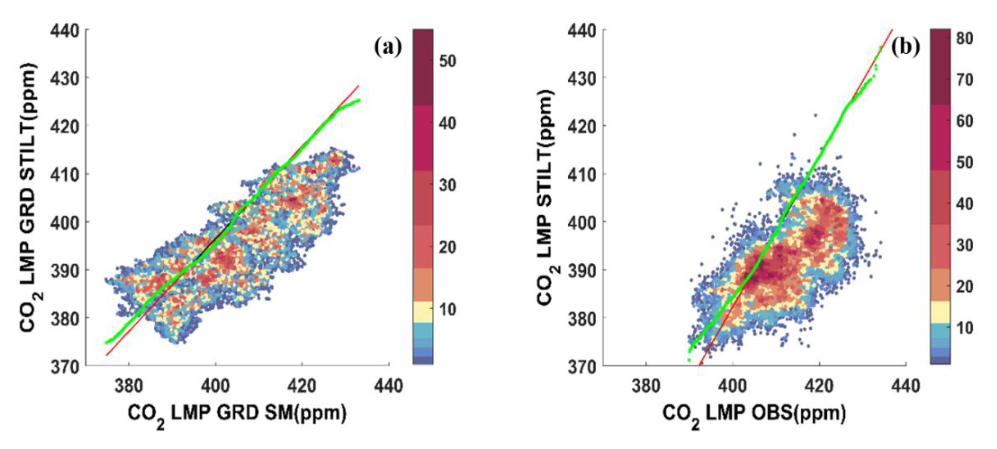
For CO2 (ppm) in Figure 6, Figure 8 and Figure 10 respectively for LMT, CGR and LMP, the q-q plots report the comparisons as follows: LMT (CGR, LMP) GRD STILT (y-axis) and LMT (CGR, LMP) GRD SM (x-axis) (a); LMT (CGR, LMP) STILT and LMT (CGR, LMP) OBS (b).
In the q-q plots colored squares indicate the amount of data in each 0.2×0.2 bin, the green lines represent the quantile–quantile plots, and red lines the least-square best fits. If the datasets of the compared methods came from the same distribution, the green lines of the q-q plot would be linear, which would coincide with the least squares best fit shown by a red line.
Table 1 shows the results of the error metrics used for the STILT and SM models as well as the LMT, CGR and LMP datasets of CH4 and CO2 over the time periods studied.
In detail, we reported the station, the time period observed for CH4 and CO2, the respective available observed data percentage, and the statistical parameters: the Root Mean Square Error (RMSE) (eq. 1), the arithmetic mean value of the errors (BIAS) (eq. 2), the Scatter Index (SI) (eq. 3), and the correlation coefficient (R2) (eq. 4).
Figure 5.
Quantile–quantile plots of CH4 hourly mean values over the 2015-2023 period, between (a) LMT STILT background (GRD) (y-axis) and LMT GRD SM datasets (x-axis); (b) LMT STILT (y-axis) and complete LMT observed (OBS) datasets (x-axis); colored squares indicate the amount of data in each 0.2×0.2 bin. Green lines represent the quantile–quantile plots, and red lines the least-square best fits.
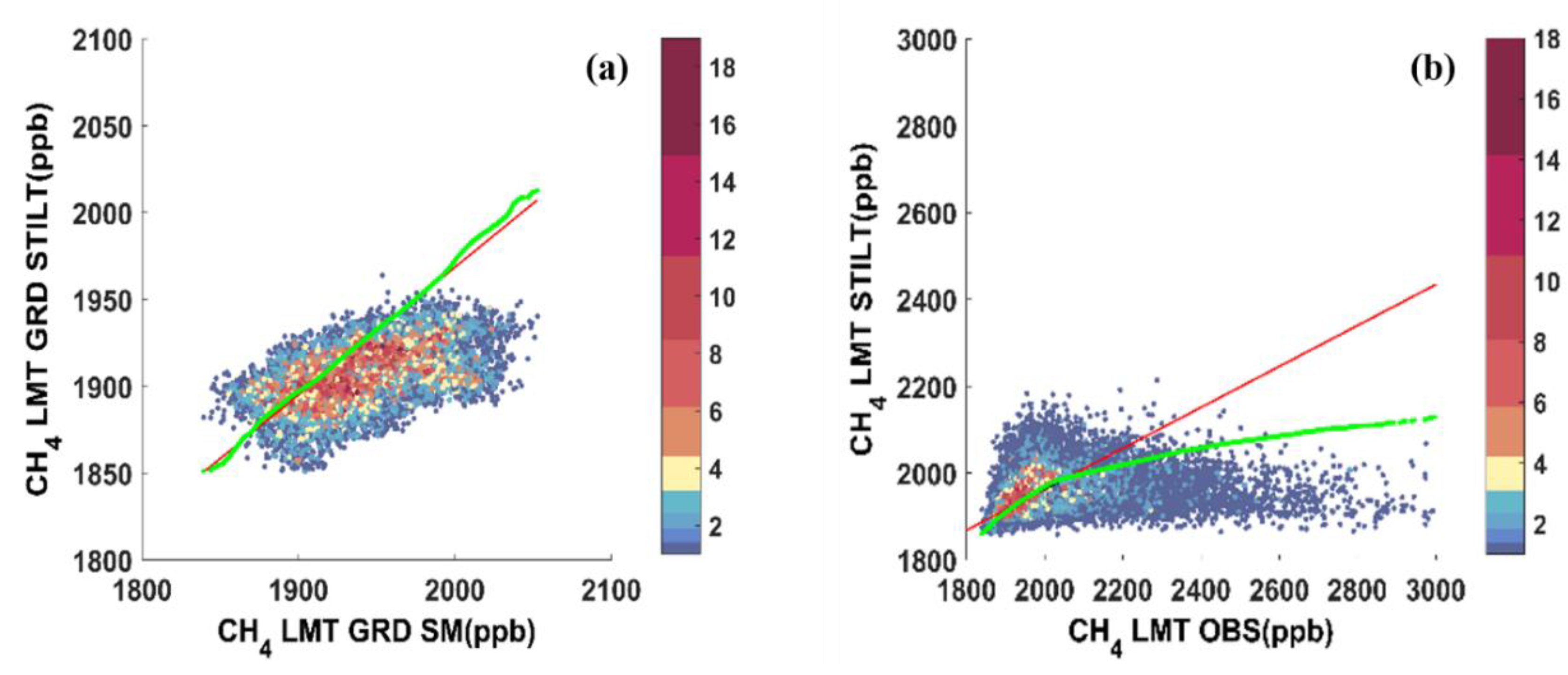
Figure 6.
Quantile–quantile plots of CO2 hourly mean values over the 2015-2023 period, between (a) LMT STILT background (GRD) (y-axis) and LMT GRD SM datasets (x-axis); (b) LMT STILT (y-axis) and complete LMT observed (OBS) datasets (x-axis); colored squares indicate the amount of data in each 0.2×0.2 bin. Green lines represent the quantile–quantile plots, and red lines the least-square best fits.
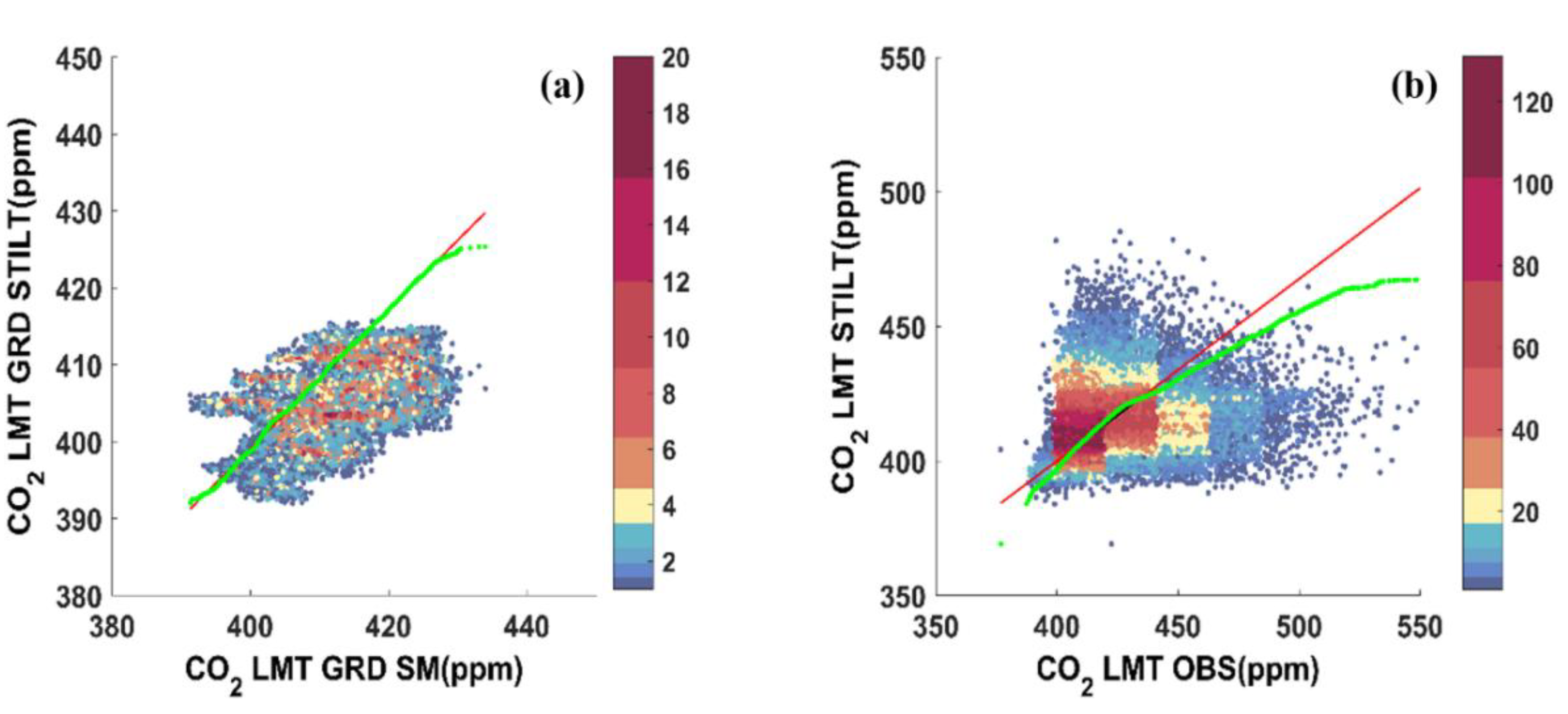
Figure 7.
Quantile–quantile plots of CH4 hourly mean values over the 2015-2022 period, between (a) CGR STILT background (GRD) (y-axis) and CGR GRD SM datasets (x-axis); (b) CGR STILT (y-axis) and complete CGR observed (OBS) datasets (x-axis); colored squares indicate the amount of data in each 0.2×0.2 bin. Green lines represent the quantile–quantile plots, and red lines the least-square best fits.
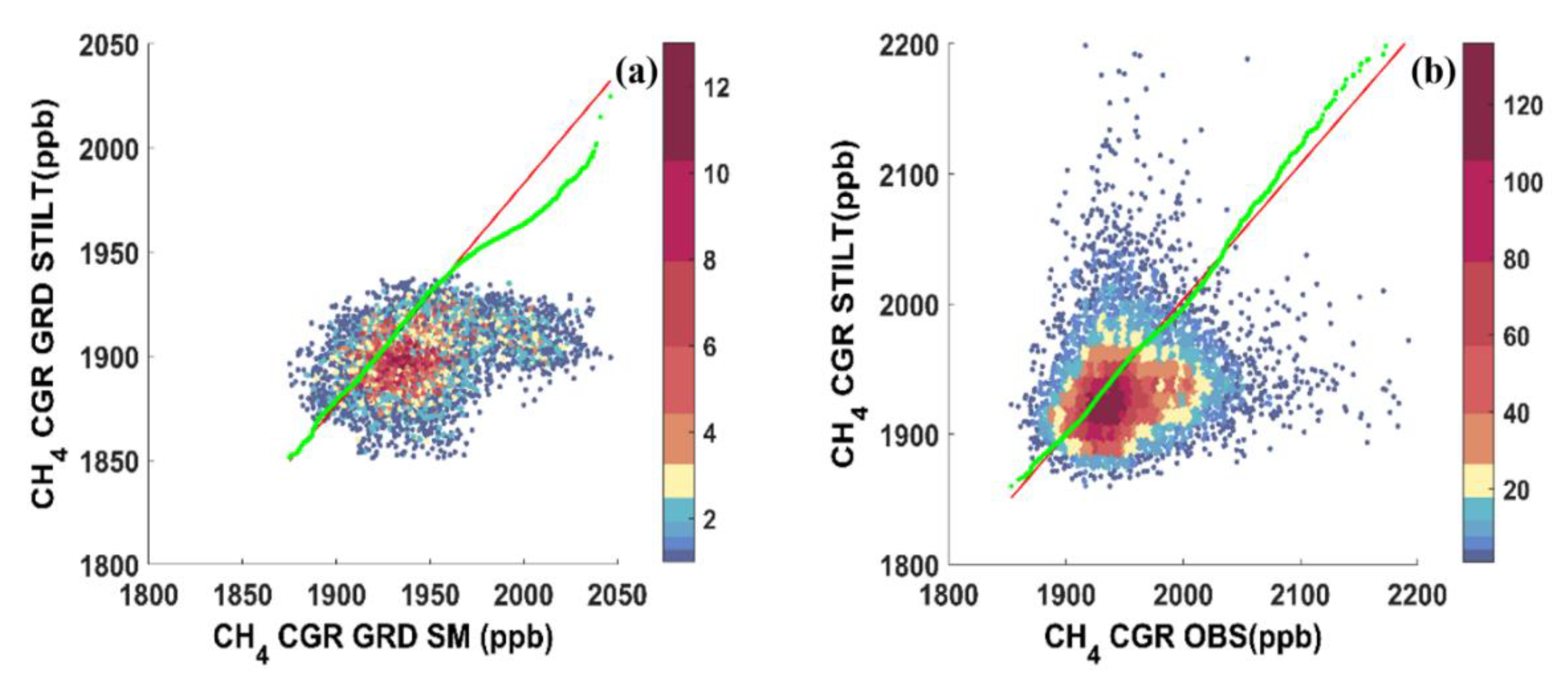
Figure 8.
Quantile–quantile plots CO2 hourly mean values over the 2015-2022 period, between (a) CGR STILT background (GRD) (y-axis) and CGR GRD SM datasets (x-axis); (b) CGR STILT (y-axis) and complete CGR observed (OBS) datasets (x-axis); colored squares indicate the amount of data in each 0.2×0.2 bin. Green lines represent the quantile–quantile plots, and red lines the least-square best fits.
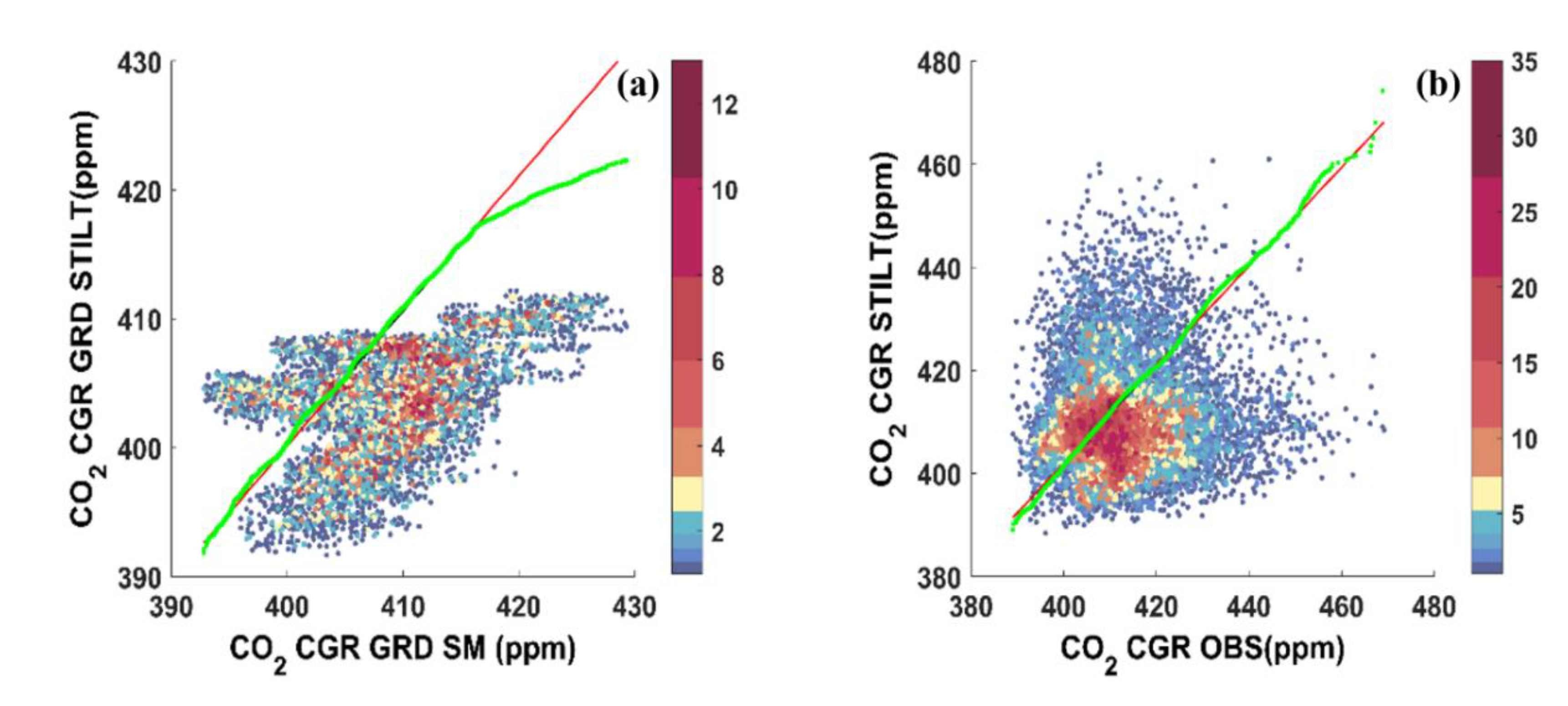
Figure 9.
Quantile–quantile plots of CH4 hourly mean values over the 2020-2024 period, between (a) LMP STILT background (GRD) (y-axis) and LMP GRD SM datasets (x-axis); (b) LMP STILT (y-axis) and complete LMP observed (OBS) datasets (x-axis); colored squares indicate the amount of data in each 0.2×0.2 bin. Green lines represent the quantile–quantile plots, and red lines the least-square best fits.
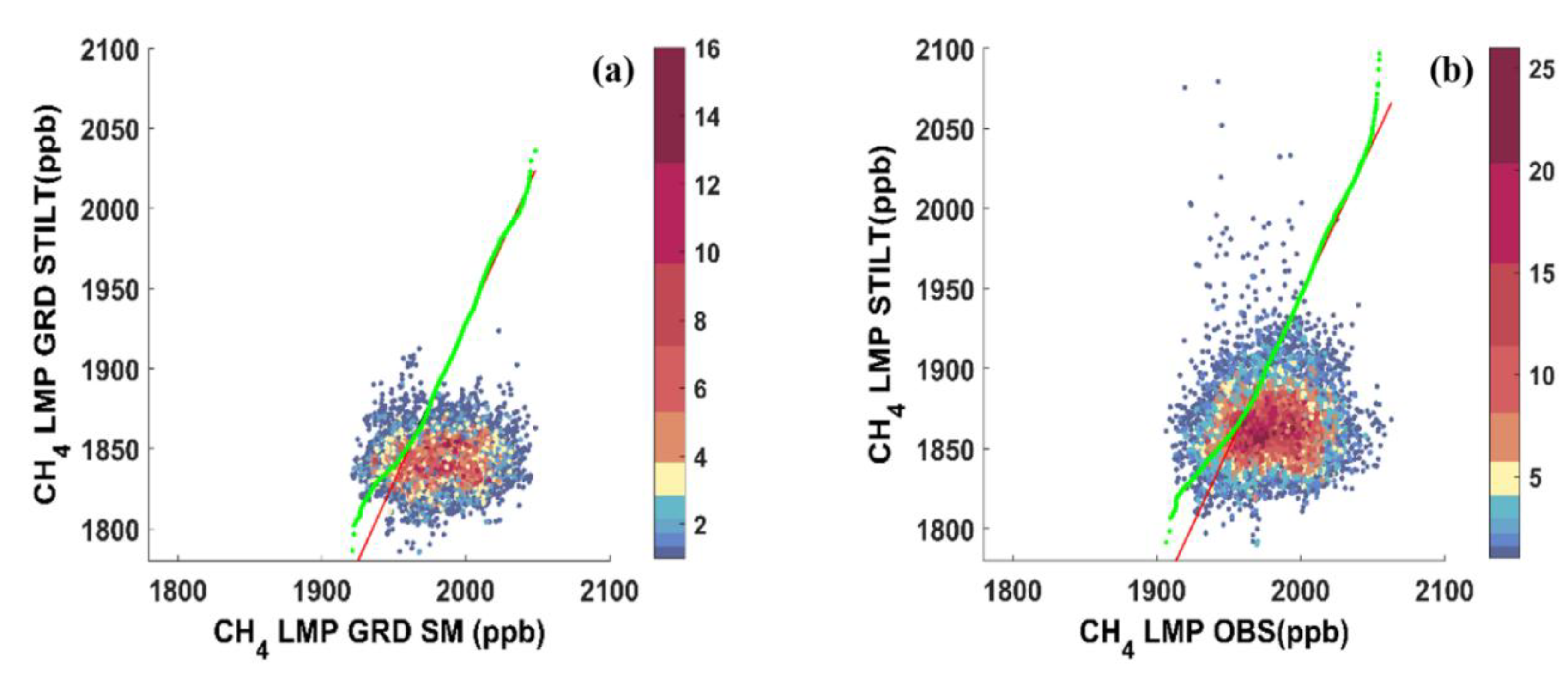
Figure 10.
Quantile–quantile plots of CO2 hourly mean values over the 2006-2024 period, between (a) LMP STILT background (GRD) (y-axis) and LMP GRD SM datasets (x-axis); (b) LMP STILT (y-axis) and complete LMP observed (OBS) datasets (x-axis); colored squares indicate the amount of data in each 0.2×0.2 bin. Green lines represent the quantile–quantile plots, and red lines the least-square best fits.
The highest RMSE values are shown in the LMT (CGR) STILT - LMT (CGR) OBS comparisons for both analyzed gases: CH4 yields 164.28 (52.18), while CO2 yields 138.84 (14.07). For CH4 and CO2, all comparisons highlight negative BIAS values, indicating an underestimation of SM background values relative to STILT background, and an underestimation of observed mole fraction values detected at three stations, relative to STILT datasets. The R2 values obtained from the comparisons reported in Table 1 do not indicate high correlations. The values are below 0.7.
The scatter index, SI, indicates the degree of discrepancy between the two distributions being compared. The smaller the value, the more similar the distributions are to each other and vice versa. Looking at the percentages of SI reported in Table 1, we can see how the values between the comparisons of the background data (GRD STILT vs GRD SM) and the no background data (STILT vs OBS), for CH4 and CO2, are very similar for CGR and LMP.
For LMT, the difference is greater (CH4 GRD: 2.42%; CH4 no GRD: 8.13%; CO2 GRD: 2.39%; CO2 no GRD: 32.41%). In relation to their position, these results are attributable to the characteristics of the individual sites.
5. Discussion
In order to verify whether the STILT simulations on background and complete datasets for LMT, CGR and LMP, are comparable with observed datasets, we report in Figure 2, Figure 3 and Figure 4 the CH4 and CO2 time series for LMT, CGR, and LMP respectively. Monthly mean values are reported here with hourly mean values as the basis. It is worth comparing the background datasets obtained by the STILT model with the background datasets attained by the SM method applied at coastal (LMT and CGR) and marine (LMP) stations datasets. This is the first work testing the SM background method implemented in Malacaria et al. (Malacaria et al., 2025) on stations with different characteristics. Notably, multi-annual tendencies for CH4 and CO2 are upward for LMT (Figure 2a,b), CGR (Figure 3a,b), and LMP (Figure 4a,b). For the three stations studied, the annual growth rate of CH4 is consistent with global measurements by the National Oceanic and Atmospheric Administration (NOAA), https://gml.noaa.gov/ccgg/trends_ch4/ (accessed on November 2024).
Consistent with the literature (Malacaria et al., 2025; Trisolino et al., 2021) and https://gml.noaa.gov/ccgg/trends/ (accessed on November 2024), there is a well-defined multi-year upward tendency for CO2. The seasonal CH4 and CO2 cycles were a combination of different contributions such as biosphere emissions, removal processes, uptake phenomena, atmospheric transport as well as agricultural fire residues (Malacaria et al., 2024) and anthropogenic emissions at different spatial and temporal scales.
In order to compare the background and the complete gases datasets for LMT, CGR, and LMP, we report in Figure 5, Figure 6, Figure 7, Figure 8, Figure 9 and Figure 10 the error metrics described in Section 3.4 to visualize the dispersion of the quantile-quantile plots related to the hourly means of CH4 and CO2.
For LMT, the quantile-quantile plots of CH4 between LMT GRD STILT vs LMT GRD SM datasets (Figure 5a) and LMT STILT vs LMT OBS (Figure 5b) showed a linear relationship coinciding with the least squares best fits in the 1850-2000 ppb range, where the highest number of measurements are located (red in bar colors). For CH4 > 2000 ppb, both comparisons show a strong drift: this is attributed to the low density of available data. Furthermore, the quantile-quantile plots of CH4 for CGR (Figure 7a,b) and for LMP (Figure 9a,b) reported a linear behavior in the range between 1900-1950 ppb and 1950-2000 ppb, respectively; a slight drift in the least-squares best fit is observed for values higher than 1950 ppb for CGR and 2000 ppb for LMP. For this last station, the comparisons in Figure 9a,b are relatable both in terms of concentration range (1800-2100 ppb) and best fit. The drift in (a) and (b) q-q plots, for CH4 concentrations > 2000 ppb is not significant due to the ground conditions at the experimental site. For LMT (CGR and LMP), the quantile-quantile plots of CO2 in Figure 6a,b (Figure 8a,b and Figure 10a,b), showed a linear relationship coinciding with the least squares best fits between 390 and 430 ppm (395-415 ppm and 400-430 ppm). For CO2 > 430 ppm (LMT and LMP) and for CO2 > 415 ppm (CGR) both comparisons in each figure show a drift. For CO2, the drifts in LMT q-q plots (Figure6a,b) against CGR and LMP are similarly pronounced.
Quantile-quantile plots are a useful way of exploring distributional analysis of gas datasets. By comparing the integrals of two probability density functions in a single plot, quantile-quantile plotting methods were able to capture the scale, location, and skewness of a dataset.
For each station, the comparisons between the STILT datasets (background and no background) and the observed datasets (SM background and no background) denote an underestimation of the observed datasets (x-axis in q-q- plots) relative to the STILT datasets (y-axis in q-q plots) because the BIAS values are negative, as reported in Table 1.
This underestimation is much more evident in LMT (see Figure 2, Figure 5 and Figure 6) compared to CGR and LMP, because LMT is more affected by events of anthropogenic nature due to its geographical location. As a marine site, LMP is more of a background monitor of gas concentrations rather than being associated with occasional events. The underestimation is also partly related to the spatial resolution grid of the model (10 km x 10 km), therefore CH₄ and CO₂ data for the three sites from the STILT model may be different from the observations.
The goodness of the implementation of the background method (SM), introduced and described by Malacaria et al. (Malacaria et al., 2025), is highlighted in this work with the search for ground data on observed datasets of CH4 and CO2 at CGR and LMP. As the latter is a marine site, the air masses come mainly from the sea and are therefore less subject to anthropogenic pollution. Therefore, comparisons with the STILT background dataset are hereby deemed the most appropriate, and the results are similar (see Figure 4a,b). With the exception of an overall underestimation in all comparisons (background and no-background), the STILT model datasets, which have been validated at the three sites, show satisfactory results and demonstrates that the model can accurately estimate the CH4 and CO2 concentrations in the Mediterranean basin.
6. Conclusion
This work describes the identification of background data using Stochastic Time Inverted Lagrangian Transport, STILT and Smoothed Minima, SM methods known from the literature on the experimental CH4 and CO2 datasets recorded at the WMO/GAW stations of Lamezia Terme (LMT), Capo Granitola (CGR) and Lampedusa (LMP) (Southern Italy).
For each station, we directly compare the background and no-background datasets of CH4 and CO2. The main results of this research will be useful to the existing information on the analysis of CH4 and CO2 variability and on the model comparison in the Mediterranean basin.
Here we present the observed CH4 and CO2 datasets registered at the LMT (between 2015 and 2023), CGR (between 2015 and 2022) and LMP (for CH4: between 2020 and 2024; for CO2: between 2006 and 2024) WMO/GAW stations.
Time-reversed Lagrangian particle dispersion modeling is an effective way to determine the atmospheric trace gas concentrations observed at ground stations. STILT has been widely used for interpretation of greenhouse gas observations. Simulations in STILT show results consistent with observed GHG datasets. The model demonstrates high fidelity simulations of hourly surface data from point measurements at CGR and LMP, with somewhat less satisfactory performance at the LMT coastal site, where anthropogenic events, such as biomass burning and anthropic sources, contribute significantly. The contribution of such events is relatively low for CGR and LMP stations. The variability of CH4 and CO2 over time at all three stations obtained by comparing the background (GRD) datasets, GRD STILT vs GRD SM, are similar, highlighting the goodness of the models (SM and STILT).
The spatial coverage of the atmospheric network needs to be extended to Southern and Western Europe by adding new continuous monitoring stations, increasing the sampling frequency of vertical profiles through the peplosphere (or planetary boundary layer, PBL) and aloft, and finally optimizing the selection of atmospheric data. In order to quantitatively link observed tracer distributions to surface emissions and to address issues of environmental concern, accurate modelling of atmospheric transport is essential. In conclusion, our study shows that the high resolution STILT model is able to provide very detailed information on trace gases from three different stations.
Author Contributions
Conceptualization, Luana Malacaria and Teresa Lo Feudo; Formal analysis, Luana Malacaria and Teresa Lo Feudo; Investigation, Luana Malacaria, Teresa Lo Feudo and Claudia Roberta Calidonna; Data curation, Luana Malacaria, Giorgia De Benedetto, Salvatore Sinopoli, Teresa Lo Feudo, Salvatore Piacentino, Paolo Cristofanelli, Maurizio Busetto, Alcide Giorgio di Sarra and Claudia Roberta Calidonna; Writing—original draft, Luana Malacaria, Teresa Lo Feudo, and Claudia Roberta Calidonna; Writing review & editing, Luana Malacaria, Giorgia De Benedetto, Salvatore Sinopoli, Teresa Lo Feudo, Ivano Ammoscato, Daniel Gullì, Francesco D’Amico and Claudia Roberta Calidonna; Supervision, Claudia Roberta Calidonna; Code developer, Giorgia De Benedetto. All authors have read and agreed to the published version of the manuscript.
Funding
This research was funded by AIR0000032 – ITINERIS (MUR PNRR MISS. 4, COMP. 2, INV. 3.1), the Italian Integrated Environmental Research Infrastructures System (D.D. n. 130/2022 - CUP B53C22002150006) under the EU - Next Generation EU PNRR - Mission 4 “Education and Research” - Component 2: “From research to business” - Investment 3.1: “Fund for the realization of an integrated system of research and innovation infrastructures”, and was partly developed under PIR01_0019 PRO-ICOS-MED and CIR0019 PRO-ICOS-MED Project (MUR PON R&I 2014-2020).
Data Availability Statement
Data are accessible, through CNR-ISAC data policy and registration at https://adc.isac.cnr.it/, and other useful links https://data.icos-cp.eu/portal/#%7B%22filterCategories%22:%7B%22station%22:%5B%22iAS_LMP%22%5D%7D%7D.
Acknowledgements
ICOS activities were supported by Joint Research Unit ICOS Italy, funded by Ministry of University and Researches, throughout CNR-DSSTTA and PRO ICOS MED Strengthening the ICOS-Italy observation network in the Mediterranean - Strengthening Human Capital PIR01_00019/CIR01_00019.
Conflicts of Interest
The authors declare no competing interests. The authors declare that they have no known competing financial interests or personal relationships that could have appeared to influence the work reported in this paper.
References
- Aksoy, H.; Kurt, I.; Eris, E. : Filtered smoothed minima baseflow separation method. Journal of Hydrology 2009, 372, 94–101. [Google Scholar] [CrossRef]
- Artuso, F.; Chamard, P.; Piacentino, S.; Sferlazzo, D.M.; De Silvestri, L.; di Sarra, A.; Meloni, D.; Monteleone, F. : Influence of transport and trends in atmospheric CO2 at Lampedusa. Atmospheric Environment 2009, 43, 3044–3051. [Google Scholar] [CrossRef]
- Artuso, F.; Chamard, P.; Piacentino, S.; di Sarra, A.; Meloni, D.; Monteleone, F.; Sferlazzo, D.M.; Thiery, F. : Atmospheric methane in the Mediterranean: Analysis of measurements at the island of Lampedusa during 1995–2005. Atmospheric Environment 2007, 41, 3877–3888. [Google Scholar] [CrossRef]
- Batesa, J.T.; Pennington, A.F.; Zhaia, X.; Friberg, M.D.; Metcalf, F.; Darrow, L.; Strickland, M.; Mulholland, J.; Russell, A. : Application and evaluation of two model fusion approaches to obtain ambient air pollutant concentrations at a fine spatial resolution (250m) in Atlanta. Environmental Modelling and Software 2018. [Google Scholar] [CrossRef]
- Calidonna, C.R.; Avolio, E.; Gullì, D.; Ammoscato, I.; De Pino, M.; Donateo, A.; Lo Feudo, T. : Five years of dust episodes at the Southern Italy GAW Regional Coastal Mediterranean Observatory: Multisensors and modeling analysis. Atmosphere 2020, 11(5), 456. [Google Scholar] [CrossRef]
- Canadell, J.G.; Le Que´ re, C.; Raupach, M.R.; Field, C.B.; Buitenhuis, E.T.; Ciais, P.; Conway, T.J.; Gillett, N.P.; Houghton, R.A.; Marland, G. : Contributions to accelerating atmospheric CO2 growth from economic activity, carbon intensity, and efficiency of natural sinks. Proceedings of the National Academy of Sciences of the USA 2007, 104(47), 18866–18870. [Google Scholar] [CrossRef]
- Chamard, P.; Thiery, F.; di Sarra, A.; Ciattaglia, L.; DE Silvestri, L.; Grigioni, P.; Monteleone, F.; Piacentino, S. : Interannual variability of atmospheric CO2 in the Mediterranean: measurements at the island of Lampedusa. Tellus 2003, 55B, 83–93. [Google Scholar] [CrossRef]
- Conway, T.J.; Tans, P.P.; Waterman, L.S.; Thoning, K.W. : Evidence for the interannual variability of the carbon cycle from the national oceanic and atmospheric Administration/Climate monitoring and Diagnostics laboratory global air sampling network. Journal of Geophysical Research 1994, 99(D11), 22831–22855. [Google Scholar] [CrossRef]
- Cristofanelli, P.; Busetto, M.; Calzolari, F.; Ammoscato, I.; Gullì, D.; Dinoi, A.; Calidonna, C.R.; Contini, D.; Sferlazzo, D.; Di Iorio, T.; Piacentino, S. : Investigation of reactive gases and methane variability in the coastal boundary layer of the central Mediterranean basin. Elem. Sci. Anth 2017, 5, 12. [Google Scholar] [CrossRef]
- D’Amico, F.; Ammoscato, I.; Gullì, D.; Avolio, E.; Lo Feudo, T.; De Pino, M.; Cristofanelli, P.; Malacaria, L.; Parise, D.; Sinopoli, S.; De Benedetto, G.; Calidonna, C.R. : Integrated analysis of methane cycles and trends at the WMO/GAW station of Lamezia Terme (Calabria, Southern Italy). Atmosphere 2024, 15(8), 946. [Google Scholar] [CrossRef]
- D’Amico, F.; Ammoscato, I.; Gullì, D.; Avolio, E.; Lo Feudo, T.; De Pino, M.; Cristofanelli, P.; Malacaria, L.; Parise, D.; Sinopoli, S.; De Benedetto, G.; Calidonna, C.R. : Anthropic-Induced Variability of Greenhouse Gasses and Aerosols at the WMO/GAW Coastal Site of Lamezia Terme (Calabria, Southern Italy): Towards a New Method to Assess the Weekly Distribution of Gathered Data. Sustainability 16(18), 8175. [CrossRef]
- D’Amico, F.; Ammoscato, I.; Gullì, D.; Avolio, E.; Lo Feudo, T.; De Pino, M.; Cristofanelli, P.; Malacaria, L.; Parise, D.; Sinopoli, S.; De Benedetto, G. : Trends in CO, CO2, CH4, BC, and NOx during the First 2020 COVID-19 Lockdown: Source Insights from the WMO/GAW Station of Lamezia Terme (Calabria, Southern Italy). Sustainability 16(18), 8229. [CrossRef]
- D’Amico, F.; Gullì, D.; Lo Feudo, T.; Ammoscato, I.; Avolio, E.; De Pino, M.; Cristofanelli, P.; Busetto, M.; Malacaria, L.; Parise, D.; Sinopoli, S.; De Benedetto, G.; Calidonna, C. : Cyclic and Multi-Year Characterization of Surface Ozone at the WMO/GAW Coastal Station of Lamezia Terme (Calabria, Southern Italy): Implications for Local Environment, Cultural Heritage, and Human Health. Environments 11(10), 227. [CrossRef]
- D’Amico, F.; Calidonna, C.R.; Ammoscato, I.; Gullì, D.; Malacaria, L.; Sinopoli, S.; De Benedetto, G.; Lo Feudo, T. : Peplospheric influences on local greenhouse gas and aerosol variability at the Lamezia Terme WMO/GAW regional station in Calabria, Southern Italy: a multiparameter investigation. Sustainability 2024, 16(23), 10175. [Google Scholar] [CrossRef]
- Donateo, A.; Lo Feudo, T.; Marinoni, A.; Dinoi, A.; Avolio, E.; Merico, E.; Calidonna, C.R.; Contini, D.; Bonasoni, P. : Characterization of in situ aerosol optical properties at three observatories in the Central Mediterranean. Atmosphere 2018, 9(10), 369. [Google Scholar] [CrossRef]
- Donateo, A.; Lo Feudo, T.; Marinoni, A.; Calidonna, C.R.; Contini, D.; Bonasoni, P. : Long-term observations of aerosol optical properties at three GAW regional sites in the Central Mediterranean. Atmospheric Research 2020, 241, 104976. [Google Scholar] [CrossRef]
- Duncan, B.N.; West, J.J.; Yoshida, Y.; Fiore, A.M.; Ziemke, J.R. : The influence of European pollution on ozone in the Near East and northern Africa. Atmos. Chem. Phys. 2008, 8, 2267–2283. [Google Scholar] [CrossRef]
- European Environment Agency. The impact of international shipping on European air quality and climate forcing, Technical report 4/2013. 2013. [Google Scholar]
- Etheridge, D.M.; Steele, L.P.; Francey, R.J.; Langenfelds, R.L. : Atmospheric methane between 1000 A.D. and present: Evidence of anthropogenic emissions and climatic variability. J. Geophys. Res. Atmos. 103, 15979–15993. [CrossRef]
- Farquhar, G.D.; von Caemmerer, S.; Berry, J.A. : A biochemical model of photosynthetic CO2 assimilation in leaves of C3 species. Planta 1980, 149, 78–90. [Google Scholar] [CrossRef]
- Farquhar, G.D.; Ehleringer, J.R.; Hubick, K.T. : Carbon Isotope Discrimination and Photosynthesis. Annual Review of Plant Physiology and Plant Molecular Biology 1989, 40, 503–537. [Google Scholar] [CrossRef]
- Federico, S.; Pasqualoni, L.; De Leo, L.; Bellecci, C. : A study of the breeze circulation during summer and fall 2008 in Calabria, Italy. Atmos. Res. 2010, 97, 1–13. [Google Scholar] [CrossRef]
- Federico, S.; Pasqualoni, L.; Sempreviva, A.M.; De Leo, L.; Avolio, E.; Calidonna, C.R.; Bellecci, C. : The seasonal characteristics of the breeze circulation at a coastal Mediterranean site in South Italy. Adv. Sci. Res. 4, 47–56. [CrossRef]
- Ferretti, D.F.; Miller, J.B.; White, J.W.C.; Etheridge, D.M.; Lassey, K.R.; Lowe, D.C.; Macfarling Meure, C.M.; Dreier, M.F.; Trudinger, C.M.; Van Ommen, T.D. : Unexpected changes to the global methane budget over the past 2000 years. Science 2005, 309, 1714–1717. [Google Scholar] [CrossRef]
- Forster, P.; Ramaswamy, V.; Artaxo, P.; Berntsen, T.; Betts, R.; Fahey, D.W.; Haywood, J.; Lean, J.; Lowe, D.C.; Myhre, G.; Jnganga, G.; Prinn, R.; Raga, G.; Schulz, M.; Van Dorland, R. : Intergovernmental Panel on Climate Change (IPCC), Contribution of Working Group I to the Fourth Assessment Report 2007, Changes in atmospheric constituents and in radiative forcing. In Climate Change: The Physical Science Basis; Solomon, S., Ed.; Cambridge Univ. Press: Cambridge, UK, 2007. [Google Scholar]
- Friedlingstein, P.; O'Sullivan, M.; Jones, M.W.; Andrew, R.M.; Bakker, D.C.E.; Hauck, J.; Landschützer, P.; Le Quéré, C.; Luijkx, I.T.; Peters, G.P.; et al. Global Carbon Budget 2023 Earth Syst. Sci. Data 15, 5301–5369.
- Gao, S.; Yang, W.; Zhang, H.; Sun, Y.; Mao, J.; Ma, Z.; Cong, Z.; Zhang, X.; Tiana, S.; Azzi, M.; Chen, L.; Bai, Z. : Estimating representative background PM2.5 concentration in heavily polluted areas using baseline separation technique and chemical mass balance model. Atmospheric Environment 2018, 174, 180–187. [Google Scholar] [CrossRef]
- Gerbig, C.; Lin, J.C.; Wofsy, S.C.; Daube, B.C.; Andrews, A.E.; Stephens, B.B.; Bakwin, P.S.; Grainger, C.A. : Toward constraining regional-scale fluxes of CO2 with atmospheric observations over a continent: 2. Analysis of COBRA data using a receptor-oriented framework. Journal of Geophysical Research Atmospheres 2003. [Google Scholar] [CrossRef]
- Giorgi, F.; Lionello, P. : Climate change projections for the Mediterranean region. Glob Planet Chang 2008, 63, 90–104. [Google Scholar] [CrossRef]
- Hall, B.D.; Crotwell, A.M.; Kitzis, D.R.; Mefford, T.; Miller, B.R.; Schibig, M.F.; Tans, P.P. : Revision of the World Meteorological Organization Global Atmosphere Watch (WMO/GAW) CO2 calibration scale. Atmos. Meas. Tech. 14, 3015–3032. [CrossRef]
- Henne, S.; Furger, M.; Nyeki, S.; Steinbacher, M.; Neininger, B.; de Wekker, S.F.J.; Dommen, J.; Spichtinger, N.; Stohl, A.; Prévôt, A. : Quantification of topographic venting of boundary layer air to the free troposphere. Atmos. Chem. Phys. 4, 497–509. [CrossRef]
- Keeling, C.D.; Bacastow, R.B.; Bainbridge, A.E.; Ekdahl, C.A.; Guenther, P.R.; Waterman, L.S.; Chin. J.F.S.: Atmospheric carbon dioxide variations at Mauna Loa observatory. Hawaii, Tellus 1976, 28(6), 538–551. [Google Scholar] [CrossRef]
- Keeling, C.D.; Mook, W.G.; Tans, P.P. : Recent trends in the 13C/12C ratio of atmospheric carbon dioxide. Nature 1979, 277, 121–123. [Google Scholar] [CrossRef]
- Keeling, C.D. : The Suess effect: 13Carbon-14Carbon interrelations. Environ Int. 1979, 2(4-6), 229–300. [Google Scholar] [CrossRef]
- Keeling, C.D.; Whorf, T.P.; Wahlen, M.; Van der Plicht, J. : Interannual extremes in the rate of rise of atmospheric carbon dioxide since 1980. Nature 1995, 375, 666–670. [Google Scholar] [CrossRef]
- Keeling, R.F. : Recording earth’s vital signs. Science 2008, 319, 1771–1772. [Google Scholar] [CrossRef] [PubMed]
- Kenea, S.T.; Lee, H.; Joo, S.; Belorid, M.; Li, S.; Labzovskii, L.D.; Park, S. : Characteristics of STILT footprints driven by KIM model simulated meteorological felds: implication for developing near real-time footprints. Asian Journal of Atmospheric Environment 2023, 17, 14. [Google Scholar] [CrossRef]
- Laughner, J.L.; Neu, J.L.; Schimel, D.; Wennberg, P.O.; Barsanti, K.; Bowman, K.W.; Chatterjee, A.; Croes, B.E.; Fitzmaurice, H.L.; Henze, D.K. : Societal shifts due to COVID-19 reveal large-scale complexities and feedbacks between atmospheric chemistry and climate change. Proc. Natl. Acad. Sci. USA 2021, 118, e2109481118. [Google Scholar] [CrossRef]
- Lee, H.; Calvin, K.; Dasgupta, D.; Krinmer, G.; Mukherji, A.; Thorne, P.; Trisos, C.; Romero, J.; Aldunce, P.; Barret, K.; Blanco, G. : Synthesis report of the IPCC Sixth Assessment Report (AR6), Longer report. IPCC. 2023. Available online: https://mural.maynoothuniversity.ie/id/eprint/17733.
- Lelieveld, J.; Berresheim, H.; Borrmann, S.; Crutzen, P.J.; Dentener, F.J.; Fischer, H.; Feichter, J.; Flatau, P.J.; Heland, J.; Holzinger, R.; Korrmann, R.; Lawrence, M.G.; Levin, Z.; Markowicz, K.M.; Mihalopoulos, N.; Minikin, A.; Ramanathan, V.; Reus, M.D.; Roelofs, G.J.; Scheeren, H.A.; Sciare, J.; Schlager, H.; Schultz, M.; Siegmund, P.; Steil, B.; Stephanou, E.G.; Stier, P.; Traub, M.; Warneke, C.; Williams, J.; Ziereis, H. : Global Air Pollution Crossroads over the Mediterranean. Science 2002, 298, 794–799. [Google Scholar] [CrossRef]
- Lin, J.C.; Gerbig, C.; Wofsy, S.C.; Andrews, A.E.; Daube, B.C.; Davis, K.J.; Grainger, C.A. : A near-field tool for simulating the upstream influence of atmospheric observations: The Stochastic Time-Inverted Lagrangian Transport (STILT) model. Journal of Geophysical Research Atmospheres 2003. [Google Scholar] [CrossRef]
- Mahadevan, P.; Wofsy, S.C.; Matross, D.M.; Xiao, X.; Dunn, A.L.; Lin, J.C.; Gerbig, C.; Munger, J.W.; Chow, V.Y.; Gottlieb, E.W. : A satellite-based biosphere parameterization for net ecosystem CO2 exchange: Vegetation Photosynthesis and Respiration Model (VPRM). Global Biogeochemical Cycles 2008. [Google Scholar] [CrossRef]
- Malacaria, L.; Parise, D.; Lo Feudo, T.; Avolio, E.; Ammoscato, I.; Gullì, D.; Sinopoli, S.; Cristofanelli, P.; De Pino, M.; D’Amico, F.; Calidonna, C. : Multiparameter Detection of Summer Open Fire Emissions: The Case Study of GAW Regional Observatory of Lamezia Terme (Southern Italy). Fire 7(6), 198. [CrossRef]
- Malacaria, L.; Sinopoli, S.; Lo Feudo, T.; De Benedetto, G.; D’Amico, F.; Ammoscato, I.; Cristofanelli, P.; De Pino, M.; Gullì, D.; Calidonna, C.R. : Methodology for selecting near-surface CH4, CO, and CO2 observations reflecting atmospheric background conditions at the WMO/GAW station in Lamezia Terme, Italy. Atmospheric Pollution Research 2025, 16(Issue 7), 102515. [Google Scholar] [CrossRef]
- Mallet, M.; Dubovik, O.; Nabat, P.; Dulac, F.; Kahn, R.; Sciare, J.; Paronis, D.; Léon, J.F. : Absorption properties of Mediterranean aerosols obtained from multi-year ground-based remote sensing observations. Atmos Chem Phys. 2013, 13, 9195–9210. [Google Scholar] [CrossRef]
- Monks, P.S. : Atmospheric composition change – global and regional air quality. Atmos. Environ. 2009, 43(33), 5268–5350. [Google Scholar] [CrossRef]
- Myhre, G.; Shindell, D.; Bréon, F.M.; Collins, W.; Fuglestvedt, J.; Huang, J.; Koch, D.; Lamarque, J.F.; Lee, D.; Mendoza, B. : Anthropogenic and Natural Radiative Forcing. In Climate Change 2013: The Physical Science Basis, Contribution of Working Group I to the Fifth Assessment Report of the Intergovernmental Panel on Climate Change; Intergovernmental Panel on Climate Change: Cambridge, UK; New York, NY, USA, 2013. [Google Scholar]
- Nisbet, E.G.; Manning, M.R.; Dlugokencky, E.J.; Fisher, R.E.; Lowry, D.; Michel, S.E.; Lund Myhre, C.; Platt, S.M.; Allen, G.; Bousquet, P. : Very Strong Atmospheric Methane Growth in the 4 Years 2014–2017: Implications for the Paris Agreement. Glob. Biogeochem. Cycles 2019, 33, 318–342. [Google Scholar] [CrossRef]
- Peng, S.; Lin, X.; Thompson, R.L.; Xi, Y.; Liu, G.; Hauglustaine, D.; Lan, X.; Poulter, B.; Ramonet, M.; Saunois, M. : Wetland emission and atmospheric sink changes explain methane growth in 2020. Nature 2022, 612, 477–482. [Google Scholar] [CrossRef]
- Querol, X.; Alastuey, A.; Pey, J.; Cusack, M.; Pérez, N. : Variability in regional background aerosols within the Mediterranean. Atmos. Chem. Phys. 2009, 9, 4575–4591. [Google Scholar] [CrossRef]
- Rayner, P.J.; Law, R.M. : The interannual variability of the global carbon cycle. Tellus 1999, 51B, 210–212. [Google Scholar] [CrossRef]
- Sand, M.; Skeie, R.B.; Sandstad, M.; Krishnan, S.; Myhre, G.; Bryant, H.; Derwent, R.; Hauglustaine, D.; Paulot, F.; Prather, M. : A multi-model assessment of the Global Warming Potential of hydrogen. Nat. Commun. 2023, 4, 203. [Google Scholar] [CrossRef]
- Seinfeld, J.H.; Pandis, S.N. Atmospheric chemistry and physics: from air pollution to climate change; Wiley Interscience: New York, USA, 1998; p. 1326 pp. [Google Scholar]
- Servadio, J.L.; Lawal, A.S.; Davis, T.; Bates, J.; Russell, A.G.; Ramaswami, A.; Convertino, M.; Botchwey, N. : Demographic Inequities in Health Outcomes and Air Pollution Exposure in the Atlanta Area and its Relationship to Urban Infrastructure. J. Urban Health 2019, 96(2), 219–234. [Google Scholar] [CrossRef] [PubMed]
- Tans, P.P.; Conway, T.J.; Nakazawa, T. : Latitudinal distribution of the sources and sinks of atmospheric carbon dioxide derived from surface observations and an atmospheric transport model. Journal of Geophysical Research 1989, 94(D4), 5151–5172. [Google Scholar] [CrossRef]
- Trisolino, P.; di Sarra, A.; Sferlazzo, D.; Piacentino, S.; Monteleone, F.; Di Iorio, T.; Apadula, F.; Heltai, D.; Lanza, A.; Vocino, A.; Caracciolo di Torchiarolo, L.; Bonasoni, P.; Calzolari, F.; Busetto, M.; Cristofanelli, P. : Application of a Common Methodology to Select in Situ CO2 Observations Representative of the Atmospheric Background to an Italian Collaborative Network. Atmosphere 2021, 12, 246. [Google Scholar] [CrossRef]
- Turquety, S.; Menut, L.; Bessagnet, B.; Anav, A.; Viovy, N.; Maignan, F.; Wooster, M. : APIFLAME v1.0: high-resolution fire emission model and application to the Euro-Mediterranean region. Geos Mod Dev. 2014, 7, 587–612. [Google Scholar] [CrossRef]
- Vardag, S.N.; Gerbig, C.; Janssens-Maenhout, G.; Levin, I. : Estimation of continuous anthropogenic CO2: model-based evaluation of CO2, CO, δ13C(CO2) and Δ14C(CO2) tracer methods. Atmospheric Chemistry and Physics 2015, 15, 12705–12729. [Google Scholar] [CrossRef]
- Wilmot, T.Y.; Lin, J.C.; Wu, D.; Oda, T.; Kort, E.A. : Toward a satellite-based monitoring system for urban CO2 emissions in support of global collective climate mitigation actions. Environ. Res. Lett. 19 084029, 2024. [CrossRef]
- World Meteorological Organization Global Atmosphere Watch No. 168. Report of the 13th WMO/IAEA Meeting of Experts on CO2 concentration and related tracers measurement techniques. Boulder, Colorado, USA, 19–22 September; 2005.
Figure 1.
CNR-ISAC, LMT WMO/GAW Calabria regional site, marked by a purple dot, (38.8°N 16.2°E, 6 meters above sea level), CGR (37.6°N 12.6°E, 5 meters above sea level) marked by a yellow dot and ENEA, LMP (33.5°N 12.6°E) marked by a blue dot, in the geographical context of the Mediterranean Sea. (Google Earth 2024).
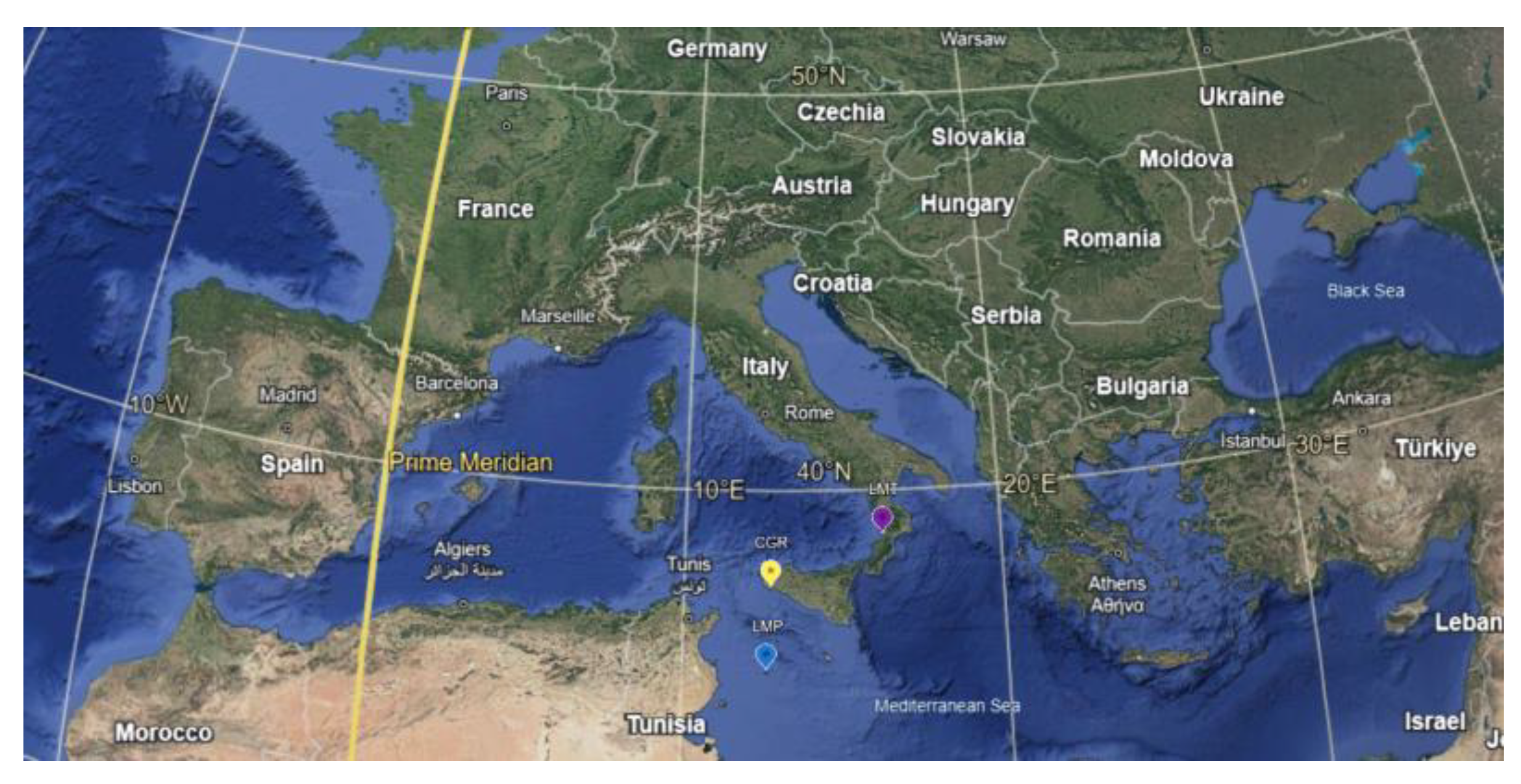
Figure 2.
CH4 (a) and CO2 (b) variability - reporting of monthly mean values of the complete Lamezia Terme (LMT) observed (LMT OBS) datasets (red line), the complete LMT STILT datasets (blue line), the LMT background SM datasets (yellow line) and the LMT background STILT datasets (purple line).
Figure 2.
CH4 (a) and CO2 (b) variability - reporting of monthly mean values of the complete Lamezia Terme (LMT) observed (LMT OBS) datasets (red line), the complete LMT STILT datasets (blue line), the LMT background SM datasets (yellow line) and the LMT background STILT datasets (purple line).
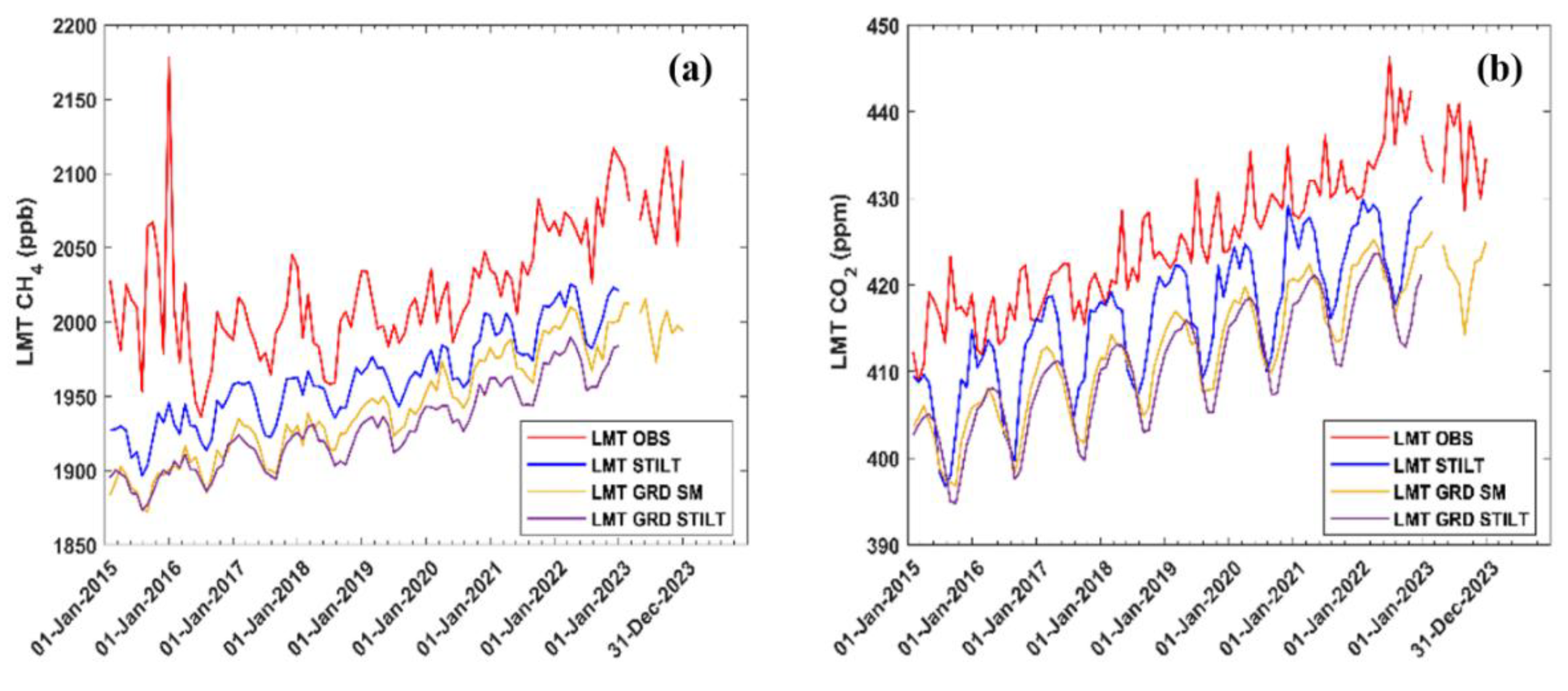
Figure 3.
CH4 (a) and CO2 (b) variability - reporting of monthly mean values of the complete Capo Granitola (CGR) observed (CGR OBS) datasets (red line), the complete CGR STILT datasets (blue line), the CGR background SM datasets (yellow line) and the CGR background STILT datasets (purple line).
Figure 3.
CH4 (a) and CO2 (b) variability - reporting of monthly mean values of the complete Capo Granitola (CGR) observed (CGR OBS) datasets (red line), the complete CGR STILT datasets (blue line), the CGR background SM datasets (yellow line) and the CGR background STILT datasets (purple line).
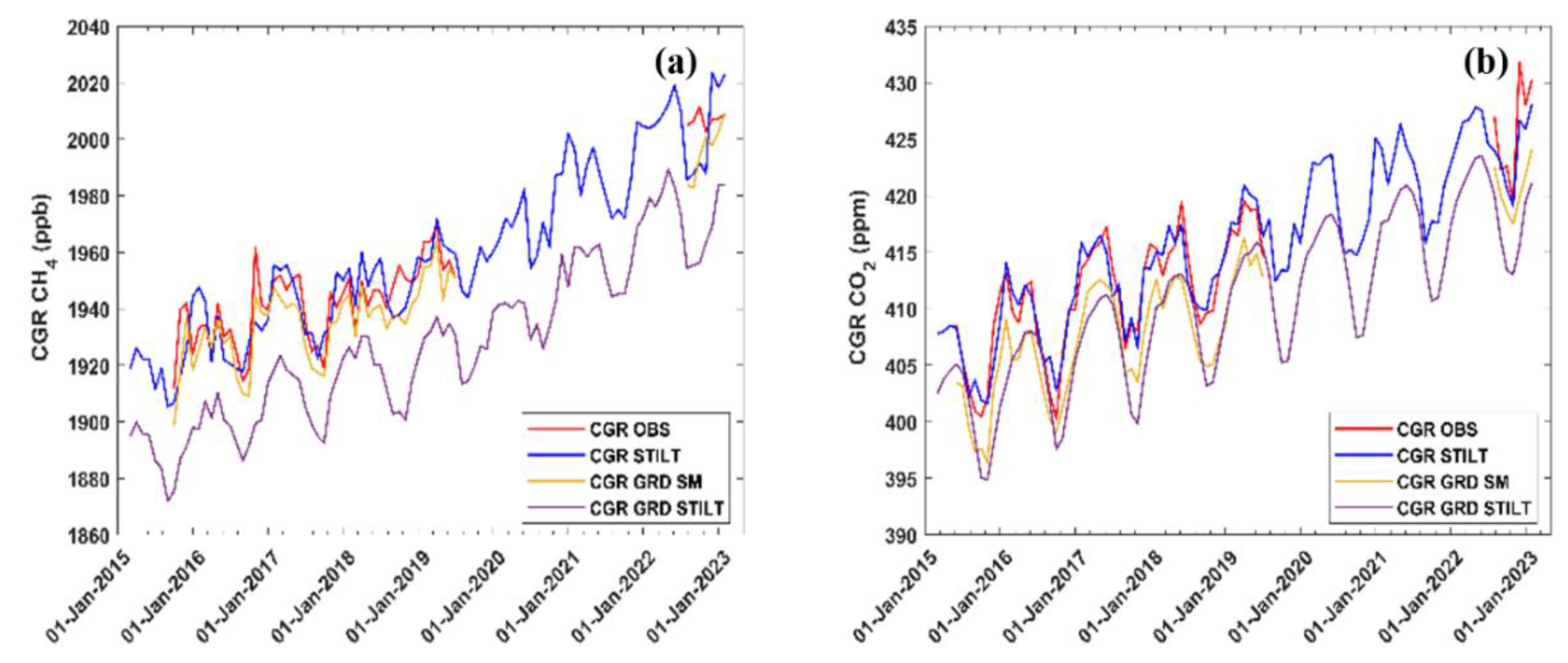
Figure 4.
CH4 (a) and CO2 (b) variability - reporting of monthly mean values of the complete Lampedusa (LMP) observed (LMP OBS) datasets (red line), the complete LMP STILT datasets (blue line), the LMP background SM datasets (yellow line) and the LMP background STILT datasets (purple line).
Figure 4.
CH4 (a) and CO2 (b) variability - reporting of monthly mean values of the complete Lampedusa (LMP) observed (LMP OBS) datasets (red line), the complete LMP STILT datasets (blue line), the LMP background SM datasets (yellow line) and the LMP background STILT datasets (purple line).
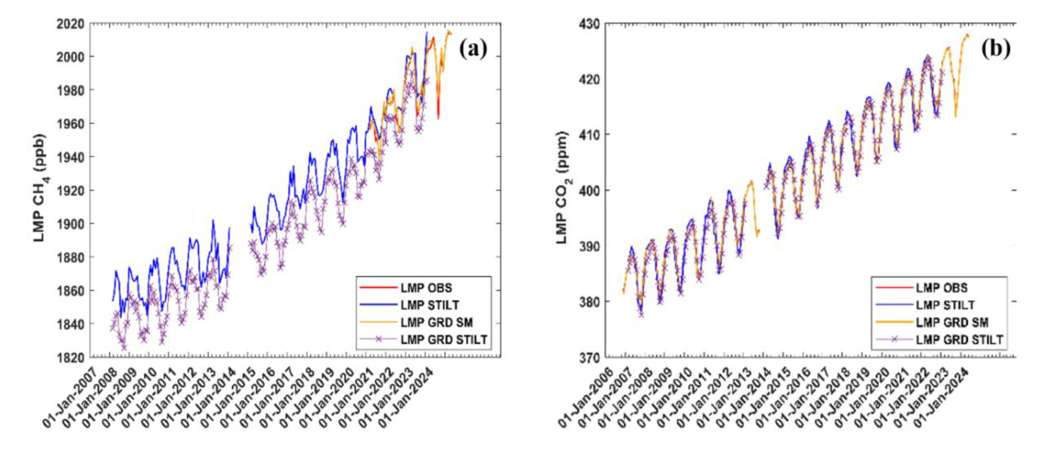

Table 1.
The error metrics used for the STILT and SM models as well as the LMT, CGR, and LMP datasets of CH4 and CO2 over the time periods studied: the Root Mean Square Error (RMSE), the arithmetic mean value of the errors (BIAS), the correlation coefficient (R2), and the Scatter Index (SI) (%).
Table 1.
The error metrics used for the STILT and SM models as well as the LMT, CGR, and LMP datasets of CH4 and CO2 over the time periods studied: the Root Mean Square Error (RMSE), the arithmetic mean value of the errors (BIAS), the correlation coefficient (R2), and the Scatter Index (SI) (%).
| Station | Time period observed | Gas | Available observed Data % | Comparison | RMSE | BIAS | R2 | SI % |
| LMT | 2015-2023 | CH4 | 91.5 | GRD STILT vs GRD SM | 46.94 | -33.77 | 0.28 | 2.42 |
| STILT vs OBS | 164.28 | -57.51 | 0.01 | 8.13 | ||||
| CO2 | GRD STILT vs GRD SM | 9.86 | -6.93 | 0.21 | 2.39 | |||
| STILT vs OBS | 138.84 | -12.15 | 0.003 | 32.41 | ||||
| CGR | 2015-2022 | CH4 | 42.8 | GRD STILT vs GRD SM | 51.63 | -44.22 | 0.10 | 2.66 |
| STILT vs OBS | 52.18 | -15.84 | 0.03 | 2.68 | ||||
| CO2 | 48.9 | GRD STILT vs GRD SM | 7.91 | -5.37 | 0.23 | 1.94 | ||
| STILT vs OBS | 14.07 | -2.46 | 0.003 | 3.41 | ||||
| LMP | 2020-2024 | CH4 | 74.7 | GRD STILT vs GRD SM | 141.78 | -139.22 | 0.006 | 7.15 |
| STILT vs OBS | 118.77 | -114.45 | 0.004 | 6.00 | ||||
| 2006-2024 | CO2 | 67.9 | GRD STILT vs GRD SM | 12.16 | -9.55 | 0.67 | 3.00 | |
| STILT vs OBS | 21.03 | -20.11 | 0.46 | 5.10 |
Disclaimer/Publisher’s Note: The statements, opinions and data contained in all publications are solely those of the individual author(s) and contributor(s) and not of MDPI and/or the editor(s). MDPI and/or the editor(s) disclaim responsibility for any injury to people or property resulting from any ideas, methods, instructions or products referred to in the content. |
© 2025 by the authors. Licensee MDPI, Basel, Switzerland. This article is an open access article distributed under the terms and conditions of the Creative Commons Attribution (CC BY) license (http://creativecommons.org/licenses/by/4.0/).
Copyright: This open access article is published under a Creative Commons CC BY 4.0 license, which permit the free download, distribution, and reuse, provided that the author and preprint are cited in any reuse.


