
Submitted:
28 March 2025
Posted:
31 March 2025
You are already at the latest version
Abstract
The Po Valley is depicted in literature as a region with one of the most severe air pollution profiles in Europe, frequently exceeding the permitted statutory concentration limits for several air pollutants. The aim of this paper is to present an assessment of the air quality over the Po Valley for the year 2022 as reported by ground-based air quality monitoring stations of the region and assess chemical transport modelling simulations which can enhance the spatiotemporal reporting in air quality levels which cannot be achieved by the sparse in situ monitoring stations coverage. To achieve this, the concentration levels of two significant chemical compounds, namely ozone (O3) and nitrogen dioxide (NO2), are studied here. Measurements include the surface concentrations of in-situ measurements from 28 stations reporting to the European Environment Agency (EEA), while chemical transport simulations from the LOng Term Ozone Simulation – European Operational Smog (LOTOS-EUROS) are employed for a comparative analysis of the relative levels observed in each of the two monitoring methods for air quality. The analysis of the EEA stations reports that, for year 2022, all selected monitoring stations exceeded the EU O3 level limit for a minimum of 33 days and the World Health Organization (WHO) limit for a minimum of 78 days. The concentrations of surface O₃ and NO₂ studied by both the measurements as well as the simulations exhibit a close correlation with the documented diurnal, monthly and seasonal variability, as previously reported in the literature. The LOTOS-EUROS CTM ozone simulations demonstrate a strong correlation with the EEA measurements, with a monthly correlation coefficient of R > 0.98 and a diurnal correlation coefficient of R > 0.83, indicating that the model is highly effective at capturing the diverse spatiotemporal patterns. The co-variability between ozone and nitrogen dioxide surface levels reported by the EEA in situ measurements reports high R values from -0.76 to -0.88 while the CTM, due to the spatial resolution of the simulations which disable the identification of local effects, reports higher correlations of -0.96 to -0.99. The CTM simulations are hence shown to be able to close the spatial gaps of the in situ measurements and provide a dependable auxiliary tool for air quality monitoring across Europe.
Keywords:
ozone
; nitrogen dioxide
; air pollution
; EEA
; LOTOS‐EUROS
; Po Valley
1. Introduction
In the post-industrial revolution times, air pollution has emerged as a dominant environmental concern, pervading numerous regions across the globe. The deterioration of air quality is primarily attributed to population growth, which has resulted in increased energy consumption and industrial production, leading to the release of considerable quantities of deleterious pollutants into the atmosphere. Such pollutants not only impair the air quality, but also have an adverse effect on ecosystems, climate and the overall quality of life [1]. It is therefore imperative to monitor air quality not only to assess immediate health risks but also to gain insight into long-term environmental impacts and to develop a more sustainable future.
In this study, the levels of two tropospheric compounds: ozone (O3) and nitrogen dioxide (NO2), are used to investigate the air-quality over the Po Valley. Tropospheric O3 is a secondary pollutant that can be transferred from the stratosphere by downward transport to the troposphere [2] and long-range transport [3] but is mainly formed when sunlight interacts with nitrogen oxides (NOx=NO2+NO), which influence the production and destruction of O3 [4], as well as with volatile organic compounds (VOCs). Similarly, the generation of O3 at the surface (ground-level O3) is also the result of the same photochemical processes as tropospheric ozone. Its variability depends on the combined effects of chemistry, transport, deposition processes [5] and the local meteorological conditions prevailing over a given region [6]. The emissions of NOx in the atmosphere originate from natural processes, primarily as a result of microbial activities in soils and lightning discharges. However, human activities, including the combustion of fossil fuels, biomass burning and the use of fertilizers, have been identified as the predominant source of NOx emissions [7].
Tropospheric ozone has a short lifetime in locations where its precursors have maximum levels, of a few hours, and up to a few weeks elsewhere, rendering it a short-lived climate gas [8,9]. The lifetime of NO2 [10,57] is also constrained to a local scale in relation to its source location and both these facts necessitate the analysis of in situ measurements in addition to the utilization modelling simulations that facilitate investigate the spatial and temporal distribution of the two compounds. Both species demonstrate a discernible diurnal pattern with O3 showing an early morning onset, a peak in the afternoon and subsequent decline in evening ozone levels. At nighttime ozone surface concentrations are measurable due to the prevalence of mechanisms that outpace ozone destruction, resulting in sustained or even elevated ozone levels. This phenomenon occurs concurrently with the cessation of photochemical production due to the absence of sunlight. The initial mechanism is the chemical reaction whereby, during nocturnal hours, specific compounds, such as peroxyacetyl nitrate (PAN), can undergo a gradual decomposition, resulting in the release of NO₂ which, in turn, reacts with O3 precursors [44]. Subsequently, NO₂ also reacts with O3 to form nitrate (NO₃) radicals, which can react with VOCs or aldehydes, forming organic nitrates that help to stabilize ozone levels [45]. Additionally, the reactions of biogenic volatile organic compounds (BVOCs), such as isoprene or terpenes, with NO₃ radicals can result in the generation of secondary organic aerosols (SOAs) and other O3 precursors [46]. Other mechanisms that contribute to the enhancement of surface ozone levels include turbulent mixing, which facilitates the transport of ozone from higher atmospheric layers to the surface [47], the mixing of O3 from the residual layer, which persists from daytime production to the surface under conditions of stable nocturnal conditions, and the horizontal transport of ozone-rich air from neighboring regions [48]. which is typically a few hours, and that of NO2 [10], which is constrained to a local scale in relation to its source location, necessitates the analysis of in situ measurements that provide data dependent on the spatiotemporal resolution, in addition to the utilization modelling simulations that facilitate the spatial and temporal distribution of the two compounds. These complex intertwined photochemical and transport processes necessitate their in tandem analysis of both these major air quality hindering species.
The study area in this work is the Po Valley, a densely inhabited region of Northern Italy, with a population of over 16 million, [11] frequently documented in the literature as one of the most significant hotspots, exceeding the air quality limit values for numerous pollutants [12,13]. The EU has adopted policies on air quality in order to decrease the exceedances for most air pollutants [14]. In particular, with regard to ozone, the Directive 2008/50/EC establishes a long-term target value of 120 μg/m³ and the WHO air quality guideline of 100 μg/m³ measured as maximum daily 8-hour running average [15].
The Po Valley has been studied in the past due to its known high air pollution levels, particularly ozone and PM10 (e.g [16]). Ozone concentrations in 1998 often exceeded in the past international regulations, with peaks reaching up to 200 ppb downwind of Milan [17]. A study examining the budget of pollutants near the surface of the Po Valley [20] concluded that, for half the year, external sources surpassed local contributions. Although local sources predominated at ground level, external contribution excess was observed 15% of the time. Given the Po Valley's topography, vertical mixing and entrainment at the boundary layer top were found to prevail over advection at low levels. The study also noted that less reactive species like CO and PM10 behaved similarly to passive tracers, while more reactive species (NO2, O3) showed pronounced seasonal and diurnal cycles due to photochemical reactivity. Long-term measurements in Modena between 1998–2010 showed that ozone concentrations have remained relatively constant despite decreasing NO levels, while PM10 exhibits strong seasonal variability with higher winter concentrations [18]. [54] investigated ozone production in the Po Valley, revealing that urban areas exhibited strongly VOC-sensitive ozone production, while rural areas showed both VOC and NOx sensitivity. Their one-dimensional Lagrangian Harvard Photochemical Trajectory Model (PTM) calculations indicated that surface-level ozone production tends to be more VOC-sensitive than the average in the mixed layer. Research also suggests an unidentified non-photochemical ground-level source of formaldehyde in the Po Valley, likely from agricultural emissions, which may contribute to ozone production [19]. While air quality modeling systems have been implemented in the past to support policy-makers [22], further improvements in emission inventories and meteorological pre-processing are needed, particularly for PM10 predictions [16].
The main aim of this paper is to assess the recent air quality situation in the Po Valley by utilizing both measurements and simulations of O₃ and NO₂, while simultaneously examining the capability of the model simulations to bridge the spatial gap of the in situ air quality measurements. The surface concentration of both pollutants is evaluated using in situ air quality measurements from European Environmental Agency (EEA) stations as well as the LOTOS-EUROS Chemical Transport Model (CTM) simulations.
The study is structured as follows. In Section 2, the area of interest and all the involved datasets are described in detail, and the methodology is presented. Section 3.1 discusses the surface air quality obtained from in situ EEA stations and LOTOS-EUROS simulations. Finally, section 4 provides a summary of the key findings of the study.
2. Data and Methodology
2.1. Area of the Po Valley
The Po Valley is considered as an approximate to a megacity in Northern Italy (Figure 1), situated on an area of about 48,000 km² [13] surrounded by the Alps to the north and the Apennines to the south, a topography which creates a microclimate that often traps pollutants [24]. The combination of urban and industrial emissions with the prevailing adverse meteorological conditions results in the accumulation of primary pollutants, such as NOx, and the formation of secondary pollutants (such as O3) in a shallow layer near the surface [23,53]. Specifically, the local atmospheric circulation features, which are dominated by calm and weak winds and the frequent temperature inversions that reduce vertical dispersion and ventilation into the free troposphere, all contribute to the development of critical pollution episodes [25].
Several studies on air pollution have been conducted over the Po Valley, with the aim of measuring the concentrations of significant pollutants. A study on the evaluation of the extent and effects of air pollution and mitigation strategies in Mestre-Venice, a large city of the Po Valley, for the period 2000-2013, revealed that CO, SO2 and benzene levels remained comparatively low and EC limit values were not exceeded, while annual average NO2 levels exceeded the EC limit in 2003 [26]. Conversely, ozone and PM10 were identified as critical pollutants, with alert thresholds and limit/objective values frequently exceeded. Another study [27] presented the long-term trend, weekly variability and cluster analysis for PM10 concentration timeseries in the Po Valley in 2014. The analysis demonstrated that PM10 concentration exhibited geographically-based differences among sites, with the main metropolitan areas being clustered along with the surrounding sites, irrespective of the station type. Finally, a three-year investigation of NO₂ pollution in the Po Valley was performed between 2018 and 2021, to analyze the impact of the lockdown on air pollution [28]. A strong correlation was identified between satellite and in situ observations of NO₂ in the Po Valley, with the majority of NO₂ pollution concentrated in the cities of Milan, Bergamo, and Brescia.
2.2. European Environment Agency Air Quality Monitoring
The database utilized for the evaluation of surface air quality is provided by the EEA. The European air quality database (https://eeadmz1-downloads-webapp.azurewebsites.net/, last accessed 20.12.2024) compiles and processes hourly measurements of several pollutants drawn from national monitoring networks across Europe and other cooperating countries.
In this study, the concentrations of O₃ and NO₂ were obtained from 28 ground-based monitoring stations distributed across the Po Valley region in northern Italy (Figure 1). The selection of the stations was based on the objective of obtaining a representative distribution of data across different zones and environments within the Po Valley, which allows the comparison of air quality across various regions. Table A1 provides additional information on the station types used herein, which have been categorized by the EEA database as follows: 19 as background urban, 3 as background suburban, one as traffic urban, two as industrial suburban and 3 as industrial rural.
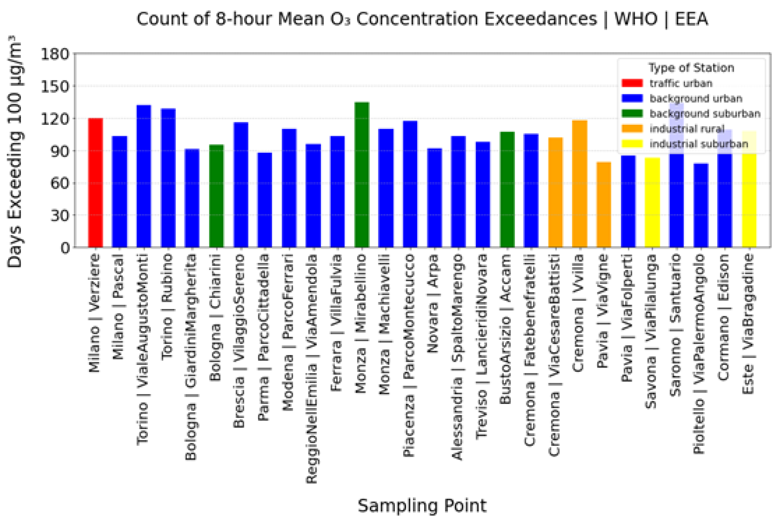
One of the key objectives of the EEA air quality database is to produce assessments that will assist the European Commission to implement EU environmental legislation in EU Member States, as well as inform European citizens about the state and outlook of Europe's air quality. In this study, the prevalence of O₃ exceedances was investigated in relation to the EU limit, as well as to the WHO Air Quality Guidelines. The results demonstrate that all selected monitoring stations exceeded the EU limit for over 33 days within the year 2022 (see Figure B1). The background urban and suburban stations demonstrate the highest frequency of exceedances, with Mirabellino station in Monza exhibiting the highest number of exceedances, surpassing 100 days. By contrast, Via Vigne station in Pavia (industrial rural) and Via Pilalunga in Este city (industrial suburban) exhibit the lowest exceedance rates, at approximately 30 days, while other stations show moderate exceedance rates. It is noteworthy that larger cities with a greater number of emission sources, such as Milano and Torino, have a higher incidence of exceedances, however the most severe cases remain in suburban areas. It is also observed that all stations exceeded the WHO limit for a minimum of 78 days within the 2022 monitoring period (see Figure B2). A study conducted in the Veneto region (North-East Italy, part of the Po Valley) over a seven-year period (2008-2014), demonstrated the existence of strong spatial gradients seasonal and diurnal trends of air pollutants (O₃, NOx) and showed that the EC long-term target value and the WHO air quality guideline were also frequently exceeded at almost all the sites [13].
2.3. LOTOS-EUROS Chemical Transport Modelling System
LOTOS-EUROS is a Eulerian 3D Chemistry Transport Model (CTM) that simulates distinct components (e.g. oxidants, primary and secondary aerosols, heavy metals) in the lower troposphere [29]. It is one of the eleven state-of-the-art models used in the Copernicus Atmospheric Monitoring Service (CAMS, http://www.copernicusatmosphere.eu, last accessed: 20.12.2024) that provides air quality forecasts of main air pollutants (ozone, NOX, PMs, SOX), affecting air quality over Europe, to a broad range of users [30]. The model has been utilized in various air quality studies, mainly for the estimation of air pollutant abundances in the lower troposphere and its performance has been extensively validated. In particular, the performance of the model has been evaluated over Greece with ground-based measurements and space-borne observations [31]. The authors demonstrated that the model reasonably reproduces the surface NO₂ concentrations in major Greek cities (R~0.8), with a mild underestimation during daytime (~11%). Moreover, modelled tropospheric NO2 columns compare well to Multi-AXis Differential Optical Absorption Spectroscopy (MAX-DOAS) measurements and TROPOspheric Monitoring Instrument (TROPOMI) observations over urban and rural areas, capturing the diurnal patterns and the spatial variability, with a small underestimation (~18%) in winter. The study [32] employed LOTOS-EUROS simulations and TROPOMI observations to derive NO2 surface concentrations over central Europe. It is found that the model performs better over background and rural areas (bias of ~20% and R > 0.65), when compared to EEA in situ measurements, but shows a difficulty in representing the sharp gradients over traffic areas (R < 0.4 and a bias > 55%). An analysis of summertime O3 over urban and rural locations in Madrid showed that LOTOS-EUROS accurately reproduced O3 surface concentrations (R~0.8 and a mean bias of ~7%) when compared to in situ measurements reporting to the local network, by incorporating high resolution meteorological data and more vertical levels in the model configuration [33]. Finally, [34] improved ozone forecasts over Europe by assimilating in situ measurements in the LOTOS-EUROS model, reporting a strong agreement (R~0.82) with ground-based measurements.
In this work, the LOTOS-EUROS v2.02.002 open-source version (https://airqualitymodeling.tno.nl/lotos-euros/open-source-version/, last accessed: 20.12.2024) is used over Northern Italy. Specifically, simulations of O3 and NO2 tropospheric surface concentrations are carried out to test the model skill over the heavily polluted Po valley. A nesting approach is configured to maximize the smooth transition of dynamics between a coarser European model run (from 15° W to 45° E and from 30° N to 60° N) with a horizontal resolution of 0.25° × 0.25° and an inner Mediterranean run (from 2° E to 35° E and from 35° N to 55° N) with a resolution of 0.1° × 0.1°. Boundary and initial conditions of the coarser European run are obtained from the CAMS global near-real time (NRT) service with a spatial resolution of 35 km × 35 km and a temporal resolution of three hours. A third nested run, centered around the Po Valley (from 6° E to 13° E and from 45° N to 50° N) with a resolution of 0.05° × 0.1° (latitude × longitude), is configured using as boundary conditions the 3-D concentration fields of the inner Mediterranean run. The model simulations are driven by operational meteorological data from the European Centre for Medium-Range Weather Forecasts (ECMWF) with a horizontal resolution of 7 km × 7 km [35]. CAMS-REG v6.1 anthropogenic emissions [36,37] for 2022, with a horizontal resolution of 0.05° × 0.1°, are ingested in the model to carry out the simulations over the Po Valley. More information on the model driving chemical and physical processes can be found at [30]. O3 and NO2 surface abundances are examined for the model pixels representative of the selected ground-based stations from the EEA network.
2.5. Methodology
The analysis commences with an assessment of surface air quality, comprising an autonomous and comparative examination of the O3 and NO2 concentrations derived from the EEA quality stations and the corresponding LOTOS-EUROS model simulations.
The initial phase of this work involves the appropriate choice of EEA-reporting air quality monitoring stations, so that they are well-distributed (geographically) across a variety of locations in the Po Valley, as well as a proper representation of different station types (see Section 2.2. for more details) that were in continuous operation throughout the year 2022. LOTOS-EUROS pixels corresponding to the locations of the final 28 air quality stations were chosen for the one-to-one comparisons shown below. In the case of the visualization of North Italy, the region bounds used for latitude were (44°N, 47°N) and longitude (7°E, 13°E), respectively.
The methodology involves the grouping of the stations based on their formal EEA classification, enabling the computation of mathematical operations and the determination of statistical values for each of the five station types: background urban, background suburban, traffic urban, industrial suburban, and industrial rural. To calculate the hourly mean, the hourly data are grouped directly by hour of the day for the entirety of 2022. This permitted then the calculation of the 8h mean levels so as to enumerate the days with exceedances for the different official limits. To calculate the daily mean, the hourly concentrations are aggregated for each calendar day while to compute the monthly averages, the daily mean concentrations are grouped by month and averaged to determine broader temporal patterns and seasonal influences throughout the year. To assess the seasonal diurnal variability, the corresponding averages are calculated by considering the mean of hourly averages within each season. The 1-sigma standard deviations (STDs) follow the calculation of the different temporal resolution averages.
3. Results
In the following sub-sections, the surface EEA air quality measurements and LOTOS-EUROS CTM simulations of O3 and NO2 over the Po Valley are first presented (section 3.1) and afterwards their co-variability is examined (section 3.1.1). The overall capacity of the CTM simulations to capture the spatiotemporal variability of ground observations is discussed throughout this section.
3.1. Surface Air Quality Assessment
In Figure 2, the annual cycle of the hourly (grey) and monthly (blue) EEA measurements for two different types of monitoring stations, traffic urban ((a), (b) panels) and industrial suburban ((c), (d) panels), are presented for ozone (a), (c), and nitrogen dioxide (b), (d). The EEA surface ozone timeseries reveal a pronounced seasonality with high levels and high variability in warmer months consistent with expectations based on photochemical processes, when solar radiation is at its highest and atmospheric photochemistry is most active [51][52]. The annual mean levels for all types of stations are presented in Table 1, left, where it is reported that the industrial suburban stations deviate from the average levels, reporting not only the highest annual mean levels, but also the highest minimum monthly mean level, pointing to a build-up of near surface ozone levels close the industrial sources.
The seasonal trend observed in the NO₂ timeseries, Figure 2, (b), (d), is notably different from that seen in ozone. This behavior is attributed to the fact that NO₂ is predominantly a byproduct of combustion processes (such as vehicle emissions and heating), which tend to be more prevalent in winter. Furthermore, photochemical reactions in the summer months facilitate the breakdown of NO₂, leading to a reduction in its concentrations during warmer periods [43]. The monthly mean corroborates the above seasonality; however, the error bars in this case show enhanced variability during the winter months due to fluctuations in emissions as well as weaker photochemically processes (e.g., heating demand or weather conditions affecting dispersion). The highest reported NO₂ concentrations, shown in Table 1, right, refer to the traffic urban stations, which also hold the highest minimum monthly mean value, pointing to a build-up of the pollutant near its source. These results are well in line with the work of [13] who examined key air pollutants (CO, NO, NO2, O3, SO2, PM10 and PM2.5) measured between 2008 and 2014 across 43 sites in the Veneto Region. They investigated seasonal and diurnal cycles and concluded that the effect of primary sources in populated areas is evident throughout the region driving similar patterns for most pollutants, while road traffic appears as the predominant potential source shaping the daily cycles. It is also worth mentioning that the data-depth classification analysis of [13] revealed a poor categorization among urban, traffic and industrial sites: weather and urban planning factors may cause a general homogeneity of air pollution within cities driving this poor classification.
Another approach to investigate air quality in the Po Valley region is to examine the O3 and NO2 surface concentrations derived from the LOTOS-EUROS simulations which offers enhanced temporal and spatial coverage, presented in Figure 3. The locations of the stations chosen in this work, as well as major coal & gas power plants, are also shown. Surface ozone concentrations are typically reduced during the winter (a) months and increased during summer (c) especially at the geographical location of the Po Valley with concentrations between ~80 and 100 μg/m3. Regarding NO₂, during winter, (b) in Figure 3, higher levels of concentrations are recorded when there are increased emissions from sources such as heating and traffic, and when atmospheric dispersion is reduced. It is important to note that, in comparison to neighboring regions, the roadside locations of the stations exhibit a higher concentrations of NO₂, for both winter and summer. The elevated concentrations observed in the vicinity of specific coal and gas power plant locations indicate the presence of localized emissions from these sources, which could potentially contribute to the deterioration of air quality, particularly in the surroundings of industrial and urban areas.
3.1.1. Monthly Mean Comparisons
In Figure 4, the monthly mean surface concentrations from the EEA in situ measurements (blue) and the LOTOS-EUROS model simulations (red) are presented for the traffic urban (a) and industrial suburban (b) stations. The data demonstrate that both lines exhibit a common seasonal variability However, quantitative analysis reveals that LOTOS-EUROS consistently overestimates ozone concentrations in winter and more specifically in the months of October and November. Additionally, the EEA dataset (blue shading) exhibits a broader range of variability compared to the LOTOS-EUROS dataset (red shading), particularly during the warmer months. This indicates that actual measurements display greater variability than the model predictions. The scatter plot comparison of the monthly mean in situ measurements and LOTOS-EUROS simulations is presented in Figure 5 for all station types. All correlation coefficients are consistently high (R > 0.98), indicating that the LOTOS-EUROS model is highly effective at capturing the temporal patterns and overall seasonal trends of ozone concentrations as already documented in [13]. The high R-values ascribe a remarkably strong agreement with the recorded concentrations by the ground-based stations. The model is highly effective in representing the measured ozone concentrations on a monthly basis and can be a reliable tool for predicting or estimating ozone concentrations, as they closely track the actual measurement.
3.1.2. Seasonal and Diurnal Comparisons
After assessing the seasonal variability, the diurnal variability per season, is examined in this subsection before proceeding to a direct comparison between surface observations and simulations.
The diurnal variability of traffic urban (a), (b) and industrial suburban (c), (d) stations is shown on a seasonal basis in Figure 6 for the EEA O3 (a), (c) and NO2 (b), (d) measurements. A pronounced diurnal variation in surface O₃ is seen with the highest levels appearing during summer months, followed by spring, autumn, and finally winter, when ozone formation is significantly reduced. The highest concentration of ozone falls within the range of ~120-140 µg/m³ and it is observed at midday, between 13:00 and 14:00 UTC, when the strength of sunlight is greatest. On the other hand, the lowest concentration ranging between ~4 and14 µg/m³ is recorded between 4:00 and 6:00 UTC. A comparative analysis of the various station types indicates that the industrial suburban stations exhibit the highest peaks and lows in ozone concentrations during the colder seasons, specifically winter (peak=44.23 μg/m3, minimum=18.04 μg/m3) and autumn (peak=70.64 μg/m3, minimum=27.45 μg/m3). A relevant study on the analysis of air pollution and climate at a background site in the Po Valley [44] showed comparable diurnal patterns for O₃ and implied that the summer diurnal pattern is significantly influenced by the enhanced dispersion induced by the warm summer weather that is typical of the Po Valley.
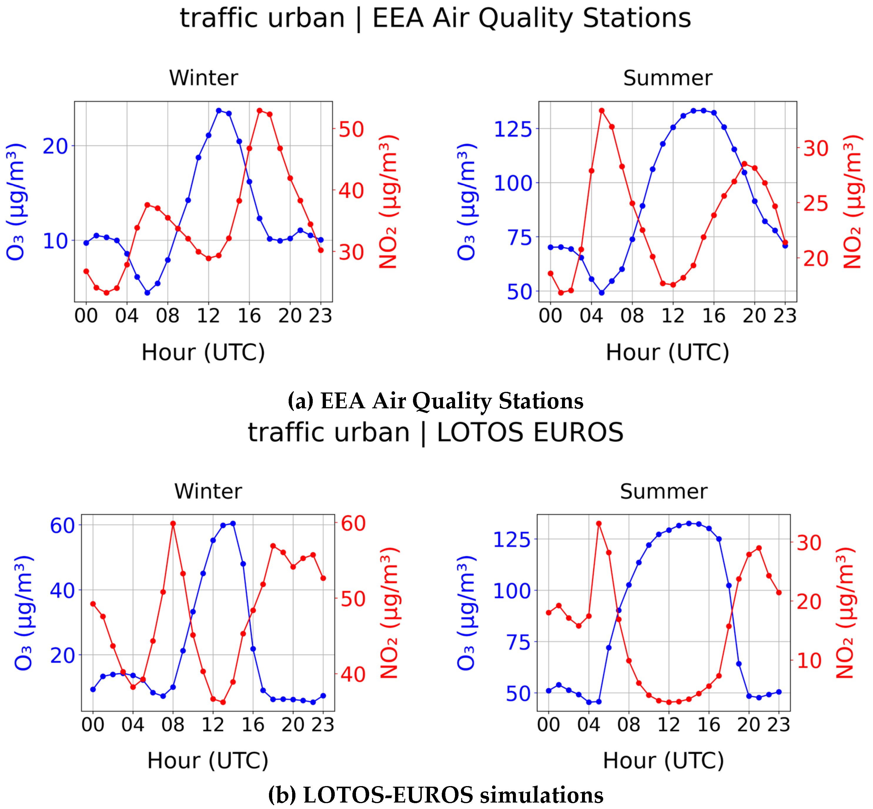
A distinct diurnal pattern is observed for NO₂ levels over the traffic urban station (Figure 6b), with two peaks in NO₂ concentration: one in the morning, occurring around 5:00 to 6:00 UTC and the other during the evening rush hour, between 18:00 and 19:00 UTC, indicating that traffic emissions have a significant impact during these times. It is noteworthy that the summertime peak occurs earlier in the morning than it does during the winter months. This phenomenon is attributed to the onset of photochemistry, which commences at an earlier time due to the earlier rising of the sun. The identified NO₂ behavior is observed in all five types of stations across all seasons examined in this study, including the industrial suburban case (Figure 6d). The industrial rural stations (not shown here) are the exception, exhibiting less pronounced diurnal fluctuations, implying that industrial zones tend to have more consistent emissions than the pulsed traffic emissions observed in urban areas. The traffic urban station exhibits the most pronounced peaks for NO₂ overall, displaying peak and minimum concentrations approximately 1.5 to 2 times larger than those observed at other station types for all seasons. In particular, during the winter season levels reach ~50 µg/m³ at 07:00 UTC (early morning) and ~60 µg/m³ at 18:00 UTC (late afternoon). Conversely, in the winter period the background suburban stations exhibit the lowest minimum value (~3 μg/m³), in stark contrast to the other station types, which display low values within the range of ~18-35 μg/m³. The presented NO₂ diurnal cycle is well in line with the findings of [18], which conclude that the double-peaked pattern observed in winter is due to traffic emissions during the rush hour periods, with the evening peak extended longer than the morning peak partly due to the higher night-time atmospheric stability as well as the decreased photochemical destruction due to insufficient sunlight.
Τhe corresponding seasonal diurnal timeseries, derived from the LOTOS-EUROS simulations, are presented in Figure 7 and reveal a discernible seasonal trend for ozone (a&c), analogous to that observed in Figure 6. The highest O3 concentrations, around 125-132 μg/m3, are observed during the summer months (red line), here reaching their peak at ~14:00 UTC, while the lowest concentrations (~5-32 μg/m3) are observed in wintertime (blue). It is noteworthy that the industrial suburban stations exhibit the highest minimum concentrations, which are approximately two to three times higher than those observed at other station types across all seasons. On the contrary, the traffic urban station consistently exhibits the lowest minimum concentrations. A review of the NO₂ diurnal variability (Figure 7b,d) reveals a similar distinct seasonal pattern across all station types to that observed in the EEA NO₂ case study. The highest concentrations are observed during winter (~30-59 μg/m³) at ~ 7:00 UTC and the lowest concentration levels are observed at ~ 13:00 UTC, throughout the summer within the range of ~1-3 μg/m³. Among station types, it is found that the traffic urban station shows the greatest peak and minimum concentrations of NO₂, reaching levels up to twice that observed in other stations. In contrast, the industrial suburban stations exhibit the lowest diurnal variability (Figure 7d).
The correlation between the seasonal urban variability measured by the insitu stations and the LE simulations datasets is highly significant, with correlation coefficients ranging between 0.83 and 0.98 and p-values near zero (Table 2) while the diurnal cycle is accurately represented by the model. Even though the winter-time correlations are the highest for all types of stations, the LE simulations result in higher morning peaks for both O3 and NO2. This fact merits further investigation since it was established that the surface levels were not influenced by probable intrusions from the free troposphere into the planetary boundary layer, which might have possibly enhanced the surface concentrations. In summary, the LOTOS-EUROS model simulations show a remarkable ability to capture the diurnal cycles of ozone across different station types and seasons and agrees well with the in situ measurements.
3.1.3. Co-Variability of Ozone and Nitrogen Dioxide Levels
This sub-section aims to provide an extensive analysis of the co-variability between O3 and NO2. In all station types for the EEA measurements, there is an inverse relationship between ozone and nitrogen dioxide, particularly during daylight hours. The measurements of the traffic urban station (Figure 9,(a)) exhibit the greatest diurnal fluctuations in NO₂ concentrations due to traffic-related emissions, while industrial and background stations (not shown here) report more uniform pollutants levels throughout the day. The LOTOS-EUROS simulations also demonstrate an inverse correlation between O₃ and NO₂, which is most pronounced during summer midday (Figure 9, (b)). The inverse relationship between O₃ and NO₂ follows a study conducted in the urban background atmosphere of Nanjing, East China [49], which demonstrated that during the summer months, the increased intensity of sunlight and elevated temperatures result in elevated rates of NO₂ photolysis, consequently leading to a more pronounced formation of ozone. This is attributed to the elevated midday O₃ levels observed during the summer season in comparison to other seasons. In winter, the reduction in sunlight and temperatures result in a decrease in photochemical activity, leading to lower ozone levels and higher NO₂ concentrations. The conditions are more favorable for the decreased photolytic breakdown of NO₂ in winter. Furthermore, [49] emphasized the pivotal role of nitrogen oxide (NO) in reducing ozone levels through the titration effect, whereby NO reacts with O₃ to form NO₂, thereby depleting ozone. This effect is particularly evident during the early morning and late evening hours, when NO concentrations are elevated due to traffic emissions and reduced photolytic activity. Consequently, lower O₃ levels are observed during these periods.
Figure 8.
Winter and summer diurnal mean surface O3 (blue) and NO2 (red) concentration (μg/m3) for the traffic urban station from EEA measurements (a) and LOTOS-EUROS simulations (b) in central Milan.
Figure 8.
Winter and summer diurnal mean surface O3 (blue) and NO2 (red) concentration (μg/m3) for the traffic urban station from EEA measurements (a) and LOTOS-EUROS simulations (b) in central Milan.
To further investigate their correlation, Figure 10 presents a scatterplot of monthly mean O3 and NO2 for all station types. As can be seen, the EEA measurements (Figure 10, (a)) exhibit a pervasive negative correlation (R) across all station types, with R values ranging from -0.76 to -0.88. The LOTOS-EUROS simulations (Figure 10, (b)) demonstrate also an inverse relationship between O3 and NO2, albeit with higher correlation coefficients (R > -0.96), indicating a stronger covariance of the simulations. This is to be expected given that the model's spatial resolution is inherently limited by the resolution of the meteorological and emissions input data. This constraint is particularly evident in traffic urban stations, where the model struggles to capture sharp concentration gradients and localized emission dynamics. Consequently, the simulated O3 and NO2 fields appear more smoothed, resulting in a stronger inverse linear relationship compared to the measured data
4. Discussion and Conclusions
Air quality assessment, at a European scale, is traditionally performed using the in situ air quality monitoring measurements reported officially to the EEA database. In recent years, chemical transport modelling has emerged as a dependable alternative which can bridge the spatial locations that the deployment of in situ stations cannot cover and hence leaving a large part of Europe under-represented in the annual reviews on the state of European air quality. In this study, the air quality over the Po Valley in northern Italy for the year 2022 was investigated using the surface concentrations of O3 and NO2 as air quality indicators. For this purpose, ground-based in situ measurements from EEA air quality stations as well as chemical transport simulations from the LOTOS-EUROS CTM were utilized. The in situ measurements are analyzed in detail in this work, to act as the “ground truth” for the assessment of the capability of the CTM to describe accurately the air quality levels of the region. In that respect, in this work we have demonstrated that:
- LOTOS-EUROS CTM simulations showed a strong correlation with EEA measurements (R > 0.98) on a monthly mean basis and R values between 0.83 and 0.98 on a seasonal diurnal temporal scale, indicating that the LOTOS-EUROS model is highly effective at capturing the spatiotemporal temporal patterns and overall seasonal trends of ozone concentrations.
- The inverse correlation between ozone and nitrogen dioxide surface levels reported by the EEA in situ measurements reports high R values from -0.76 to -0.88 while the CTM, due to the spatial resolution of the simulations which disable the identification of local effects, reports higher correlations of -0.96 to -0.99.
- The consistent overestimation of ozone concentrations during its morning peak levels in January and February 2022 identified in this work remains a point for further investigation.
With respect to the ozone-related air quality assessment based on the EEA in situ stations, it was shown that all 28 stations studied in this work exceeded the EU ozone limit for an 8h average of 120 μg/m³ for over 33 days and the WHO limit of 100 μg/m³ for more than 78 days, with the highest exceedances occurring in urban and suburban areas (Figure 10a). Displaying a similar spatial pattern, albeit in some cases with higher number of days reporting exceedances, the LOTOS-EUROS CTM simulations (Figure 10b) can provide a suitable addition to the assessment of air quality in the region.
In summary, the results of the EEA measurements and LOTOS-EUROS simulations were consistent with the seasonal variation and diurnal patterns documented in the literature for O3 and NO2. The model effectively mirrors the EEA observed ozone concentrations on a monthly scale, and its simulations may serve as a trustworthy tool for forecasting or estimating ozone levels, as they align closely with the ground-based in situ measurements.
Author Contributions
Conceptualization, M-E. K., A. G. and D. B.; methodology, M-E. K. and A. P.; software, S. M.; validation, S. M. and A. P.; formal analysis, S. M.; data curation, S. M. and A. P.; visualization, S. M. ; writing—original draft preparation, S. M., A. P. and M-E. K. ; writing—review and editing, all authors; supervision, A. G. and D. B. All authors have read and agreed to the published version of the manuscript.
Funding
This research received no external funding.
Data Availability Statement
The European Environment Agency (EEA) air quality monitoring station dataset are publicly available from https://eeadmz1-downloads-webapp.azurewebsites.net/, last access: 20.12.2024. The LOTOS-EUROS v2.3 is an open-source chemical transport model (CTM) available from https://airqualitymodeling.tno.nl/lotos-euros/open-source-version/, last access: 20.12.2024. The LOTOS-EUROS simulations shown in this article are available upon request from A.P.
Acknowledgments
Results presented in this work have been produced using the Aristotle University of Thessaloniki (AUTh) High Performance Computing Infrastructure and Resources. The authors would like to acknowledge the support provided by the IT Center of the Aristotle University of Thessaloniki (AUTh) throughout the progress of this research work.
Conflicts of Interest
The authors declare no conflicts of interest.
Appendix A

Table A1.
Selected EEA air quality monitoring stations.
| Sampling Point | Name/Locality | City | Station Type |
|---|---|---|---|
| SPO.IT0705A | Verziere | Milano | Traffic urban |
| SPO.IT0706A | Via Palermo Angolo | Pioltello | Background urban |
| SPO.IT0804A | Parco Cittadella | Parma | Background urban |
| SPO.IT0842A | V. villa | Cremona | Industrial rural |
| SPO.IT0892A | Giardini Margherita | Bologna | Background urban |
| SPO.IT0912A | Via Folperti | Pavia | Background urban |
| SPO.IT0940A | Via Amendola | Reggio N. Emilia | Background urban |
| SPO.IT1144A | Via Pilalunga | Savona | Industrial suburban |
| SPO.IT1459A | Accam | Busto Arsizio | Background suburban |
| SPO.IT1590A | Lancieridi Novara | Treviso | Background urban |
| SPO.IT1650A | Santuario | Saronno | Background urban |
| SPO.IT1692A | Pascal | Milan | Background urban |
| SPO.IT1737A | Vilaggio Sereno | Brescia | Background urban |
| SPO.IT1739A | Fatebene fratelli | Cremona | Background urban |
| SPO.IT1743A | Machiavelli | Monza | Background urban |
| SPO.IT1746A | Via Vigne | Pavia | Industrial rural |
| SPO.IT1771A | Parco Ferrari | Modena | Background urban |
| SPO.IT1830A | Spalto Marengo | Alessandria | Background urban |
| SPO.IT1871A | Via Bragadine | Este | Industrial suburban |
| SPO.IT1877A | Rubino | Torino | Background urban |
| SPO.IT1918A | Villa Fulvia | Ferrara | Background urban |
| SPO.IT1975A | Parco Montecucco | Piacenza | Background urban |
| SPO.IT2063A | Via Cesare Battisti | Cremona | Industrial rural |
| SPO.IT2075A | Chiarini | Bologna | Background suburban |
| SPO.IT2098A | Mirabellino | Monza | Background suburban |
| SPO.IT2168A | Viale Augusto Monti | Torino | Background urban |
| SPO.IT2232A | Edison | Cormano | Background urban |
| SPO.IT2282A | Arpa | Novara | Background urban |
Appendix B
Figure B1.
Days exceeding the EU Air Quality Standards for max 8-hour mean ozone concentration by city population.
Figure B1.
Days exceeding the EU Air Quality Standards for max 8-hour mean ozone concentration by city population.
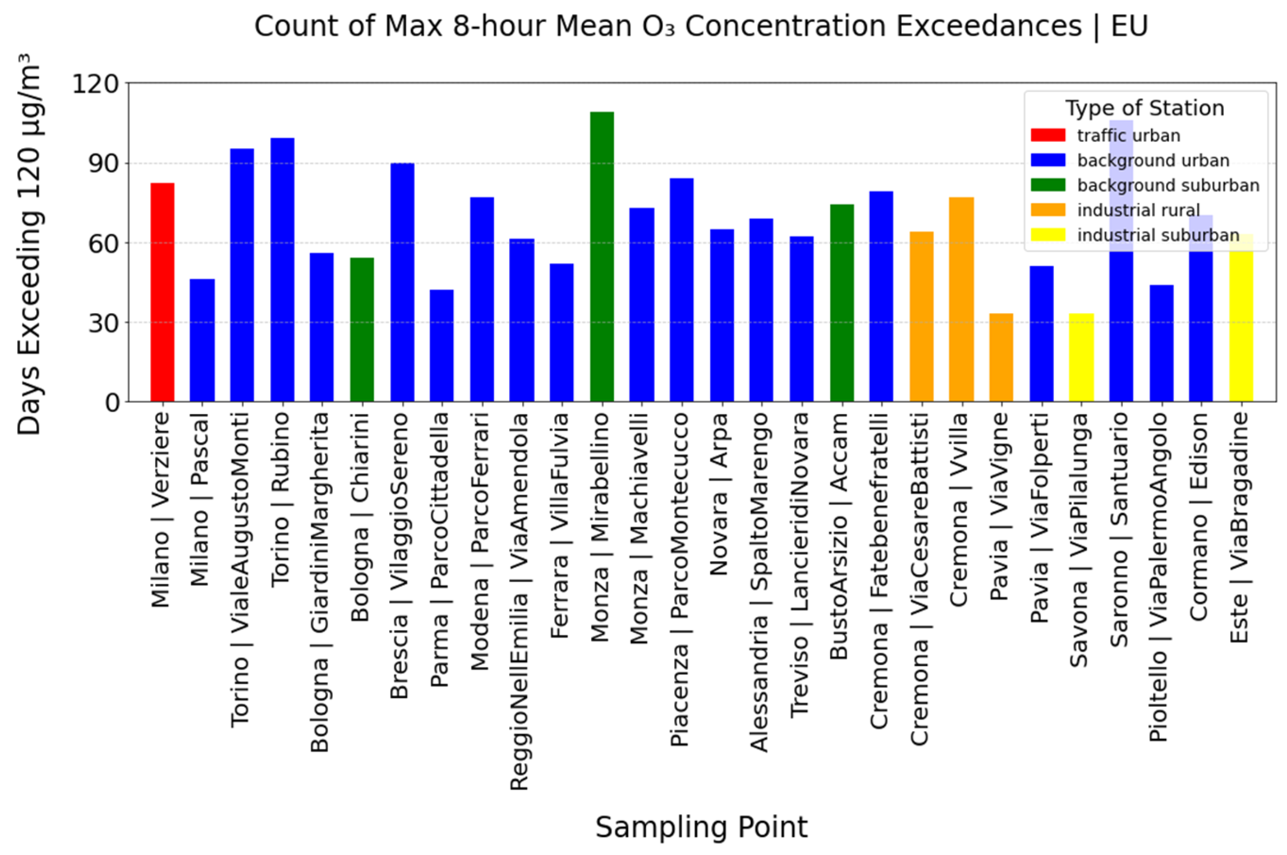
Figure B2.
Days exceeding the WHO Air Quality Guideline for 8-hour mean ozone concentration by city population.
Figure B2.
Days exceeding the WHO Air Quality Guideline for 8-hour mean ozone concentration by city population.
References
- Sharma, A.K., Sharma, M., Sharma, A.K., Sharma, M. and Sharma, M. (2023). Mapping the impact of environmental pollutants on human health and environment: A systematic review and meta-analysis. Journal of Geochemical Exploration, 255, pp.107325–107325. [CrossRef]
- Husain, L., Coffey, P.E., Meyers, R.E. and Cederwall, R.T. (1977). Ozone transport from stratosphere to troposphere. Geophysical Research Letters, 4(9), pp.363–365. [CrossRef]
- Stohl, A. and Trickl, T. (2006). Long-Range Transport of Ozone from the North American Boundary Layer to Europe: Observations and Model Results. Kluwer Academic Publishers eBooks, [online] pp.257–266. [CrossRef]
- Crutzen, P.J. (1979). The Role of NO and NO2 in the Chemistry of the Troposphere and Stratosphere. Annual Review of Earth and Planetary Sciences, 7(1), pp.443–472. [CrossRef]
- Jiang, X., Cheng, X., Liu, J., Chen, Z., Wang, H., Deng, H., Hu, J., Jiang, Y., Yang, M., Gai, C. and Cheng, Z. (2024). Comparison of Surface Ozone Variability in Mountainous Forest Areas and Lowland Urban Areas in Southeast China. Atmosphere, [online] 15(5), pp.519–519. [CrossRef]
- Lakshmi, K.A.K., Nishanth, T., Kumar, S. and Valsaraj, K.T. (2024). A Comprehensive Review of Surface Ozone Variations in Several Indian Hotspots. Atmosphere, [online] 15(7), pp.852–852. [CrossRef]
- O. Badr and S.D. Probert (1993). Oxides of nitrogen in the Earth’s atmosphere: Trends, sources, sinks and environmental impacts. Applied Energy, 46(1), pp.1–67. [CrossRef]
- Monks, P.S, A.T. Archibald, A. Colette, O. Cooper, M. Coyle, R. Derwent, D. Fowler, C. Granier, K.S. Law, G.E. Mills, D.S. Stevenson, O. Tarasova, V. Thouret, E. von Schneidemesser, R. Sommariva, O. Wild and M.L. Williams (2015). Tropospheric ozone and its precursors from the urban to the global scale from air quality to short-lived climate forcer. Atmospheric Chemistry and Physics, [online] 15(15), pp.8889–8973. [CrossRef]
- Jiang, X., Cheng, X., Liu, J., Chen, Z., Wang, H., Deng, H., Hu, J., Jiang, Y., Yang, M., Gai, C. and Cheng, Z. (2024). Comparison of Surface Ozone Variability in Mountainous Forest Areas and Lowland Urban Areas in Southeast China. Atmosphere, [online] 15(5), pp.519–519. [CrossRef]
- Koukouli, M.-E., Pseftogkas, A., Karagkiozidis, D., Skoulidou, I., Drosoglou, T., Balis, D., Bais, A.F., Melas, D. and Hatzianastassiou, N. (2022). Air Quality in Two Northern Greek Cities Revealed by Their Tropospheric NO2 Levels. 13(5), pp.840–840. [CrossRef]
- Po Valley. [online] Available at: https://geography.name/po-valley/.
- Pivato, A., Pegoraro, L., Masiol, M., Bortolazzo, E., Bonato, T., Formenton, G., Cappai, G., Beggio, G. and Giancristofaro, R.A. (2023). Long time series analysis of air quality data in the Veneto region (Northern Italy) to support environmental policies. Atmospheric Environment, [online] 298, p.119610. [CrossRef]
- Masiol, M., Squizzato, S., Formenton, G., Harrison, R.M. and Agostinelli, C. (2017). Air quality across a European hotspot: Spatial gradients, seasonality, diurnal cycles and trends in the Veneto region, NE Italy. Science of The Total Environment, 576, pp.210–224. [CrossRef]
- European Commission (n.d.). Air Quality. [online] environment.ec.europa.eu. Available at: https://environment.ec.europa.eu/topics/air/air-quality_en.
- World Health Organization (2021). What are the WHO Air quality guidelines? [online] World Health Organization. Available at: https://www.who.int/news-room/feature-stories/detail/what-are-the-who-air-quality-guidelines.
- Benassi, A., Dalan, F., Alessandro Gnocchi, Maffeis, G., Giampiero Malvasi, Liguori, F., Pernigotti, D., Pillon, S., Sansone, M. and Susanetti, L. (2011). A one-year application of the Veneto air quality modelling system: regional concentrations and deposition on Venice lagoon. International Journal of Environment and Pollution, 44(1/2/3/4), pp.32–32. [CrossRef]
- Martilli, A., A. Neftel, G. Favaro, F. Kirchner, S. Sillman, and A. Clappier, Simulation of the ozone formation in the northern part of the Po Valley, J. Geophys. Res., 107(D22), 8195, 2002. [CrossRef]
- Bigi, A., Ghermandi, G. and Harrison, R.M. (2012). Analysis of the air pollution climate at a background site in the Po valley. J. Environ. Monit., 14(2), pp.552–563. [CrossRef]
- Kaiser, J., Wolfe, G. M., Bohn, B., Broch, S., Fuchs, H., Ganzeveld, L. N., Gomm, S., Häseler, R., Hofzumahaus, A., Holland, F., Jäger, J., Li, X., Lohse, I., Lu, K., Prévôt, A. S. H., Rohrer, F., Wegener, R., Wolf, R., Mentel, T. F., Kiendler-Scharr, A., Wahner, A., and Keutsch, F. N.: Evidence for an unidentified non-photochemical ground-level source of formaldehyde in the Po Valley with potential implications for ozone production, Atmos. Chem. Phys., 15, 1289–1298, 2015. [CrossRef]
- Maurizi, A., Russo, F. and Tampieri, F. (2013). Local vs. external contribution to the budget of pollutants in the Po Valley (Italy) hot spot. Science of The Total Environment, 458-460, pp.459–465. [CrossRef]
- Lonati, G. and Riva, F. (2021). Regional Scale Impact of the COVID-19 Lockdown on Air Quality: Gaseous Pollutants in the Po Valley, Northern Italy. Atmosphere, 12(2), p.264. [CrossRef]
- Thunis, P., Triacchini, G., White, L., Maffeis, G. and Volta, M. (2009). Air pollution and emission reductions over the Po-valley: Air quality modelling and integrated assessment. [online] 18th World IMACS / MODSIM. Available at: https://mssanz.org.au/modsim09/F10/thunis.pdf [Accessed 15 Dec. 2024].
- Zhu, T., Melamed, M.L., Parrish, D., Gllardo Klenner, L., Lawrence, M., Konare, A. and Liousse, C. (eds) (2012) WMO/IGAC Impacts of Megacities on Air Pollution and Climate. Geneva: World Meteorological Organization, ISBN: 978-0-9882867-0-2, pp.299.
- Topographic-map.com (2024). Po Valley topographic map, elevation, terrain. [online] Topographic maps. Available at: https://en-us.topographic-map.com/map-6ffntf/Po-Valley/ [Accessed 15 Dec. 2024].
- Caserini, S., Giani, P., Cacciamani, C., Ozgen, S. and Lonati, G. (2017). Influence of climate change on the frequency of daytime temperature inversions and stagnation events in the Po Valley: historical trend and future projections. Atmospheric Research, 184, pp.15–23. [CrossRef]
- Masiol, M., Agostinelli, C., Formenton, G., Tarabotti, E. and Pavoni, B. (2014). Thirteen years of air pollution hourly monitoring in a large city: Potential sources, trends, cycles and effects of car-free days. Science of The Total Environment, 494-495, pp.84–96. [CrossRef]
- Bigi, A. and Ghermandi, G. (2014). Long-term trend and variability of atmospheric PM10 concentration in the Po Valley. Atmospheric Chemistry and Physics, 14(10), pp.4895–4907. [CrossRef]
- Serio, C., Masiello, G. and Cersosimo, A. (2022). NO2 pollution over selected cities in the Po valley in 2018–2021 and its possible effects on boosting COVID-19 deaths. Heliyon, 8(8), p.e09978. [CrossRef]
- Schaap, M., Timmermans, R.M.A., Roemer, M., Boersen, G.A.C., Builtjes, P.J.H., Sauter, F.J., Velders, G.J.M. and Beck, J.P. (2008). The LOTOS–EUROS model: description, validation and latest developments. International Journal of Environment and Pollution, 32(2), pp.270–290.
- Manders, A.M.M., Builtjes, P.J.H., Curier, L., Denier van der Gon, H.A.C., Hendriks, C., Jonkers, S., Kranenburg, R., Kuenen, J.J.P., Segers, A.J., Timmermans, R.M.A., Visschedijk, A.J.H., Wichink Kruit, R.J., van Pul, W.A.J., Sauter, F.J., van der Swaluw, E., Swart, D.P.J., Douros, J., Eskes, H., van Meijgaard, E. and van Ulft, B. (2017). Curriculum vitae of the LOTOS–EUROS (v2.0) chemistry transport model. Geoscientific Model Development, [online] 10(11), pp.4145–4173. [CrossRef]
- Skoulidou, I., Koukouli, M.-E., Manders, A., Segers, A., Karagkiozidis, D., Gratsea, M., Balis, D., Bais, A., Gerasopoulos, E., Stavrakou, T., Geffen, J. van, Eskes, H. and Richter, A. (2021). Evaluation of the LOTOS-EUROS NO2 simulations using ground-based measurements and S5P/TROPOMI observations over Greece. Atmospheric Chemistry and Physics, 21(7), pp.5269–5288. [CrossRef]
- Pseftogkas, A., Koukouli, M.-E., Segers, A., Manders, A., Geffen, J. van, Balis, D., Meleti, C., Stavrakou, T. and Eskes, H. (2022). Comparison of S5P/TROPOMI Inferred NO2 Surface Concentrations with In Situ Measurements over Central Europe. Remote Sensing, 14(19), p.4886. [CrossRef]
- Escudero, M., Segers, A., Kranenburg, R., Querol, X., Alastuey, A., Borge, R., de la Paz, D., Gangoiti, G. and Schaap, M. (2019). Analysis of summer O3 in the Madrid air basin with the LOTOS-EUROS chemical transport model. Atmospheric Chemistry and Physics, [online] 19(22), pp.14211–14232. [CrossRef]
- Curier, R.L., Timmermans, R., Calabretta-Jongen, S., Eskes, H., Segers, A., Swart, D. and Schaap, M. (2012). Improving ozone forecasts over Europe by synergistic use of the LOTOS-EUROS chemical transport model and in-situ measurements. Atmospheric environment, 60, pp.217–226. [CrossRef]
- Hersbach, H., Bell, B., Berrisford, P., Hirahara, S., Horányi, A., Muñoz-Sabater, J., Nicolas, J., Peubey, C., Radu, R., Schepers, D., Simmons, A., Soci, C., Abdalla, S., Abellan, X., Balsamo, G., Bechtold, P., Biavati, G., Bidlot, J., Bonavita, M. and Chiara, G. (2020). The ERA5 global reanalysis. Quarterly Journal of the Royal Meteorological Society, 146(730). [CrossRef]
- Kuenen, J., Dellaert, S., Visschedijk, A., Jalkanen, J.-P., Super, I. and Denier van der Gon, H. (2022). CAMS-REG-v4: a state-of-the-art high-resolution European emission inventory for air quality modelling. Earth System Science Data, [online] 14(2), pp.491–515. [CrossRef]
- Copernicus, E. (2023). Copernicus Atmosphere CAMS2_61 -Global and European emission inventories Documentation of CAMS emission inventory products. [online]. [CrossRef]
- www.eumetsat.int. (2020). Metop Series | EUMETSAT Website. [online] Available at: https://www.eumetsat.int/our-satellites/metop-series.
- Aeris-data.fr. (2024). IASI – aeris. [online] Available at: https://www.aeris-data.fr/en/projects/iasi-2/ [Accessed 15 Dec. 2024].
- Hurtmans, D., Coheur, P.-F., Wespes, C., Clarisse, L., Scharf, O., Clerbaux, C., Hadji-Lazaro, J., George, M. and Solène Turquety (2012). FORLI radiative transfer and retrieval code for IASI. Journal of Quantitative Spectroscopy & Radiative Transfer, 113(11), pp.1391–1408. [CrossRef]
- Acsaf.org. (2024). AC SAF - IASI information. [online] Available at: https://acsaf.org/iasi.php [Accessed 15 Dec. 2024].
- Boynard, A., Hurtmans, D., Garane, K., Goutail, F., Hadji-Lazaro, J., Koukouli, M. E., Wespes, C., Vigouroux, C., Keppens, A., Pommereau, J.-P., Pazmino, A., Balis, D., Loyola, D., Valks, P., Sussmann, R., Smale, D., Coheur, P.-F., and Clerbaux, C.: Validation of the IASI FORLI/EUMETSAT ozone products using satellite (GOME-2), ground-based (Brewer–Dobson, SAOZ, FTIR) and ozonesonde measurements, Atmos. Meas. Tech., 11, 5125–5152, 2018. [CrossRef]
- Wang, X., Zhou, L., Liu, Y., Zhang, K. and Xiu, G. (2020). Investigating the photolysis of NO2 and influencing factors by using a DFT/TD-DFT method. Atmospheric Environment, 230, p.117559. [CrossRef]
- Jenkin, M.E. and Clemitshaw, K.C. (2002). Chapter 11 Ozone and other secondary photochemical pollutants: chemical processes governing their formation in the planetary boundary layer. Developments in Environmental Science, pp.285–338. [CrossRef]
- Wayne, R.P., Barnes, I., Biggs, P., Burrows, J.P., Canosa-Mas, C.E., Hjorth, J., Le Bras, G., Moortgat, G.K., Perner, D., Poulet, G., Restelli, G. and Sidebottom, H. (1991). The nitrate radical: Physics, chemistry, and the atmosphere. Atmospheric Environment. Part A. General Topics, 25(1), pp.1–203. [CrossRef]
- Atkinson, R. and Arey, J. (2003). Gas-phase tropospheric chemistry of biogenic volatile organic compounds: a review. Atmospheric Environment, 37, pp.197–219. [CrossRef]
- Stull, R.B. (2009). An introduction to boundary layer meteorology. New York: Springer.
- Jacob, D.J. (1999). Introduction to atmospheric chemistry. Princeton, New Jersey: Princeton University Press.
- Jia, M., Zhao, T., Cheng, X., Gong, S., Zhang, X., Tang, L., Liu, D., Wu, X., Wang, L. and Chen, Y. (2017). Inverse Relations of PM2.5 and O3 in Air Compound Pollution between Cold and Hot Seasons over an Urban Area of East China. Atmosphere, 8(12), p.59. [CrossRef]
- Strode, S.A., Ziemke, J.R., Oman, L.D., Lamsal, L.N., Olsen, M.A. and Liu, J. (2019). Global changes in the diurnal cycle of surface ozone. Atmospheric Environment, 199, pp.323–333. [CrossRef]
- Lu, X., Zhang, L. and Shen, L. (2019). Meteorology and Climate Influences on Tropospheric Ozone: a Review of Natural Sources, Chemistry, and Transport Patterns. Current Pollution Reports, 5(4), pp.238–260. [CrossRef]
- Sullivan, J.T., Apituley, A., Mettig, N., Kreher, K., Knowland, K.E., Allaart, M., Piters, A., Van Roozendael, M., Veefkind, P., Ziemke, J.R., Kramarova, N., Weber, M., Rozanov, A., Twigg, L., Sumnicht, G. and McGee, T.J. (2022). Tropospheric and stratospheric ozone profiles during the 2019 TROpomi vaLIdation eXperiment (TROLIX-19). Atmospheric Chemistry and Physics, [online] 22(17), pp.11137–11153. [CrossRef]
- Hakim, Z.M., Archer-Nicholls, S., Beig, G., Folberth, G.A., Sudo, K., Abraham, N.L., Ghude, S.D., Henze, D.K. and Archibald, A.T. (2019). Evaluation of tropospheric ozone and ozone precursors in simulations from the HTAPII and CCMI model intercomparisons – a focus on the Indian subcontinent. Atmospheric Chemistry and Physics, 19(9), pp.6437–6458. [CrossRef]
- Spirig, C., A. Neftel, L. I. Kleinman, and J. Hjorth, NOx versus VOC limitation of O3 production in the Po valley: Local and integrated view based on observations, J. Geophys. Res., 107(D22), 8191, 2002. [CrossRef]
- Clerbaux, C., Hadji-Lazaro, J., Solène Turquety, George, M., Boynard, A., Pommier, M., Safieddine, S., Pierre-François Coheur, Hurtmans, D., Lieven Clarisse and Martin Van Damme (2015). Tracking pollutants from space: Eight years of IASI satellite observation. Comptes Rendus Geoscience, 347(3), pp.134–144. [CrossRef]
- Keppens, A., Compernolle, S., Verhoelst, T., Hubert, D., and Lambert, J.-C.: Harmonization and comparison of vertically resolved atmospheric state observations: methods, effects, and uncertainty budget, Atmos. Meas. Tech., 12, 4379–4391, 2019. [CrossRef]
- Beirle, S., Platt, U., Wenig, M., and Wagner, T.: Weekly cycle of NO2 by GOME measurements: a signature of anthropogenic sources, Atmos. Chem. Phys., 3, 2225–2232, 2003. [CrossRef]
Figure 1.
Power plants and selected stations in Northern Italy. EEA stations are shown as colored boxes and power plants are shown as triangles.
Figure 1.
Power plants and selected stations in Northern Italy. EEA stations are shown as colored boxes and power plants are shown as triangles.
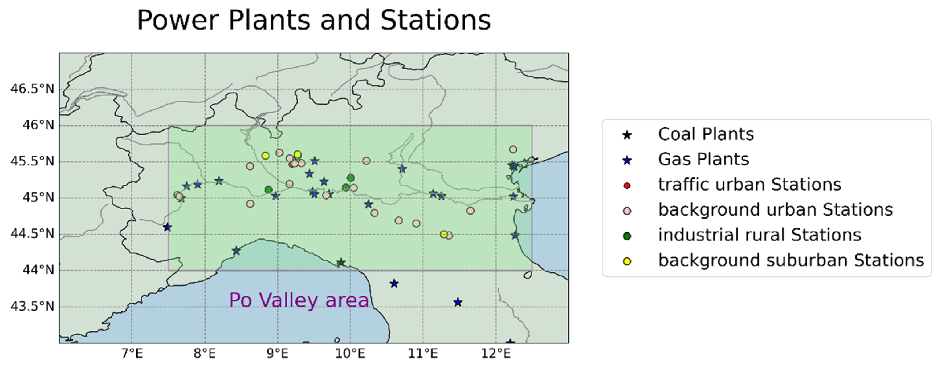
Figure 2.
Hourly (grey) and monthly (blue) mean EEA surface ozone (a), (c) and nitrogen dioxide (b), (d) concentrations (μg/m3) for the traffic urban and two industrial suburban stations over the Po Valley. The red line represents the 1-sigma error for the monthly mean concentration.
Figure 2.
Hourly (grey) and monthly (blue) mean EEA surface ozone (a), (c) and nitrogen dioxide (b), (d) concentrations (μg/m3) for the traffic urban and two industrial suburban stations over the Po Valley. The red line represents the 1-sigma error for the monthly mean concentration.
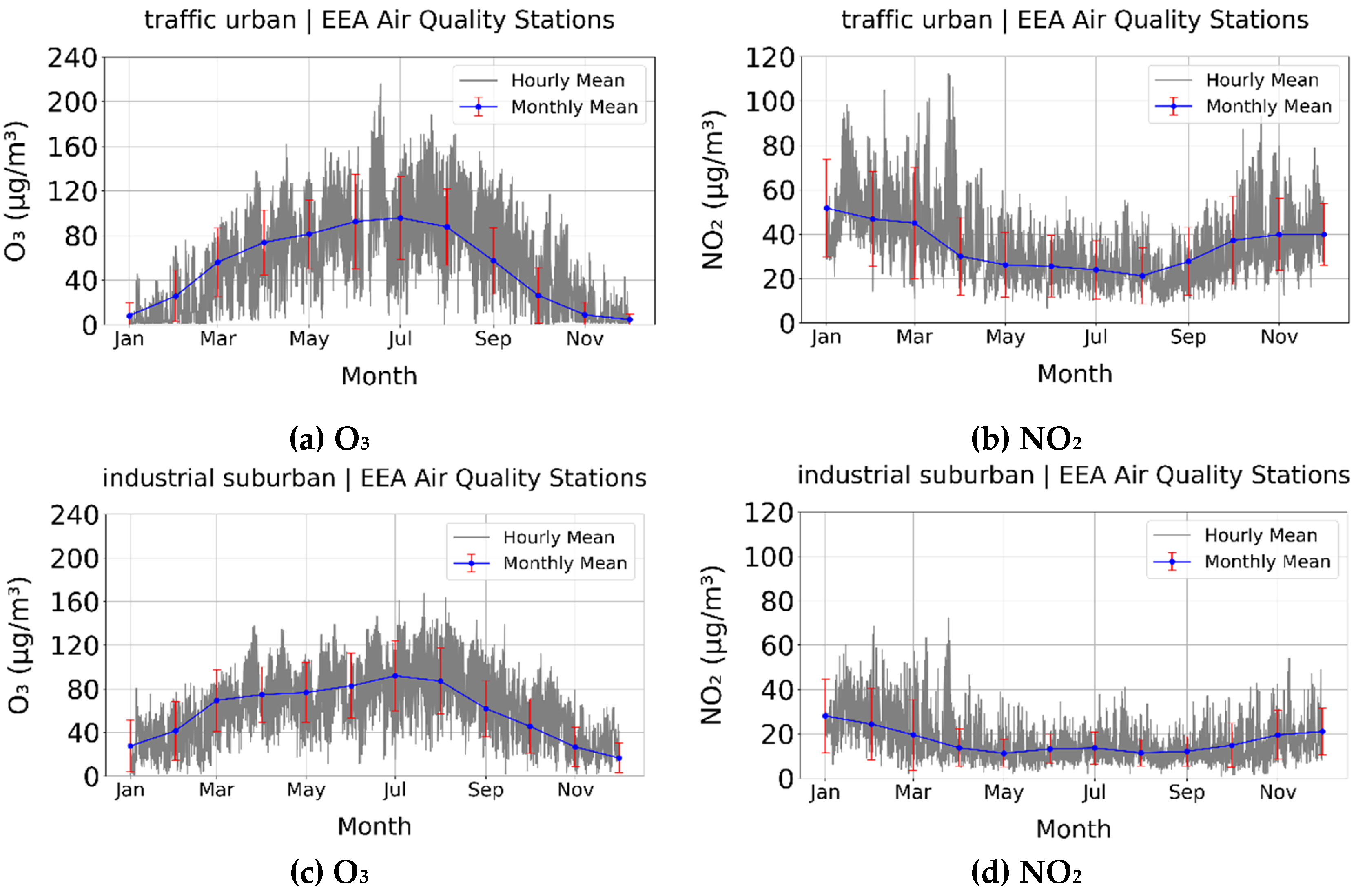
Figure 3.
Monthly mean LOTOS-EUROS surface concentrations of O3 in (a) Winter, (c) Summer and NO2 in (b) Winter, (d) Summer over North Italy. The locations of the EEA stations are given as yellow boxes and the coal and gas plants as purple triangles.
Figure 3.
Monthly mean LOTOS-EUROS surface concentrations of O3 in (a) Winter, (c) Summer and NO2 in (b) Winter, (d) Summer over North Italy. The locations of the EEA stations are given as yellow boxes and the coal and gas plants as purple triangles.
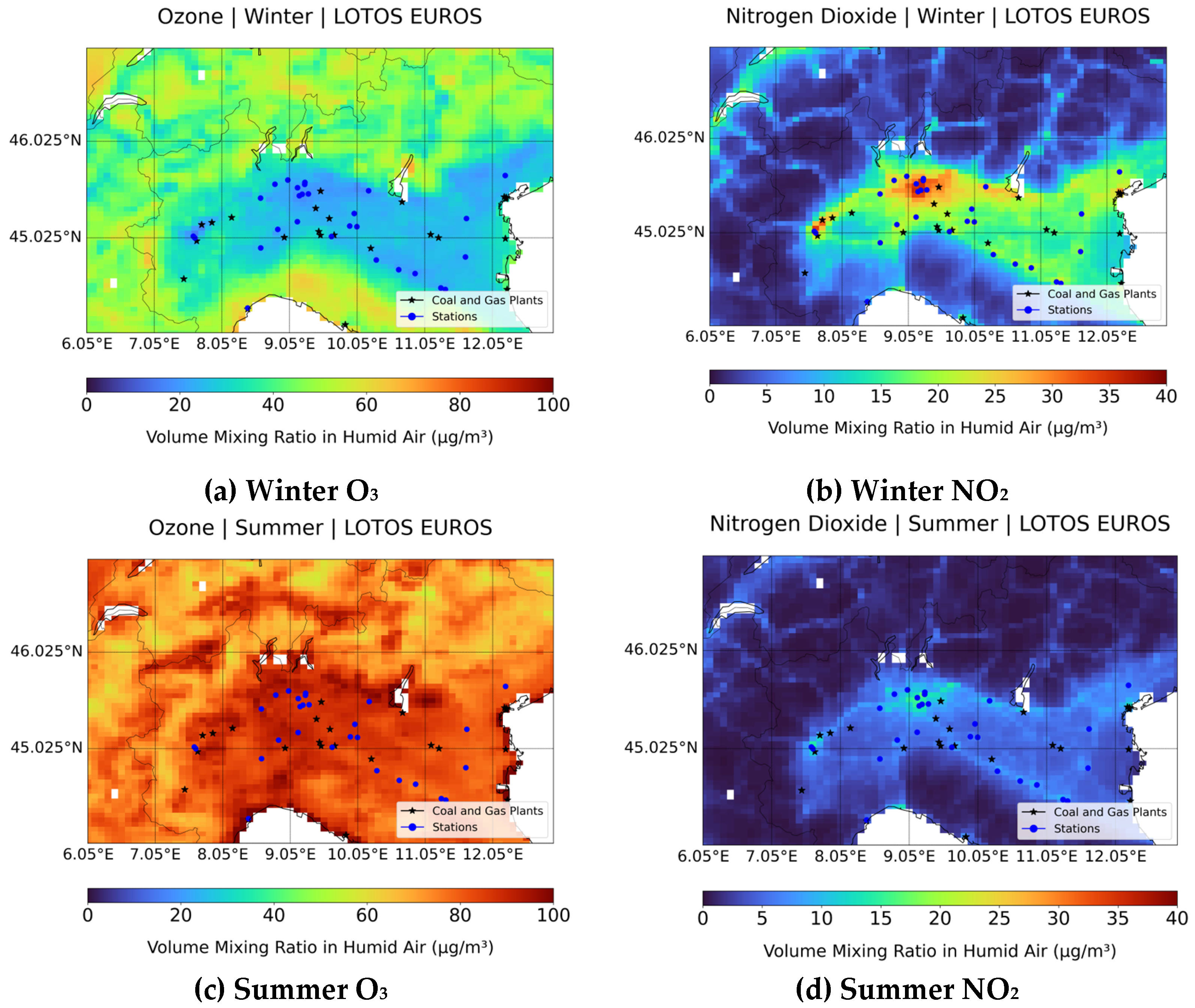
Figure 4.
Monthly mean surface EEA (blue) and LOTOS-EUROS (red) ozone concentrations (μg/m3) for the traffic urban and two industrial suburban stations over the Po Valley. The shaded areas represent the standard deviation of the monthly mean.
Figure 4.
Monthly mean surface EEA (blue) and LOTOS-EUROS (red) ozone concentrations (μg/m3) for the traffic urban and two industrial suburban stations over the Po Valley. The shaded areas represent the standard deviation of the monthly mean.
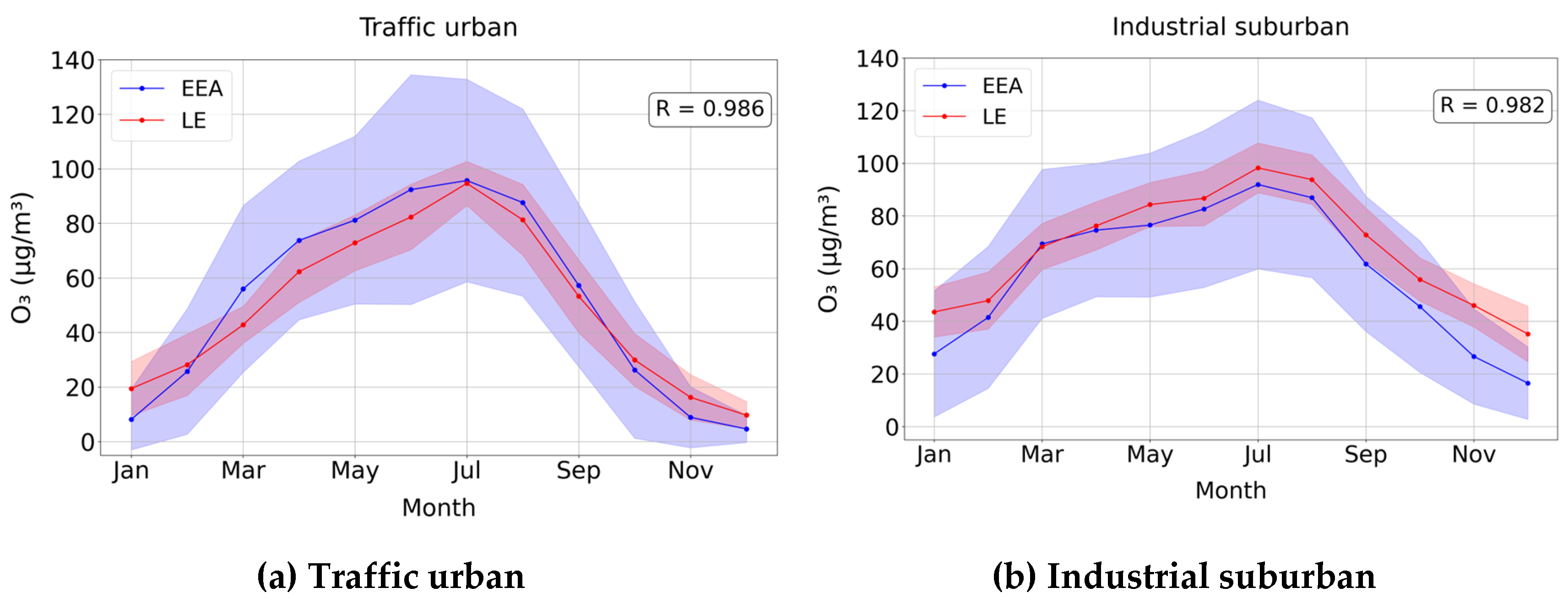
Figure 5.
Scatterplot of monthly mean surface EEA (x-axis) and LOTOS-EUROS (y-axis) ozone concentration (μg/m3) for all station types over the Po Valley.
Figure 5.
Scatterplot of monthly mean surface EEA (x-axis) and LOTOS-EUROS (y-axis) ozone concentration (μg/m3) for all station types over the Po Valley.
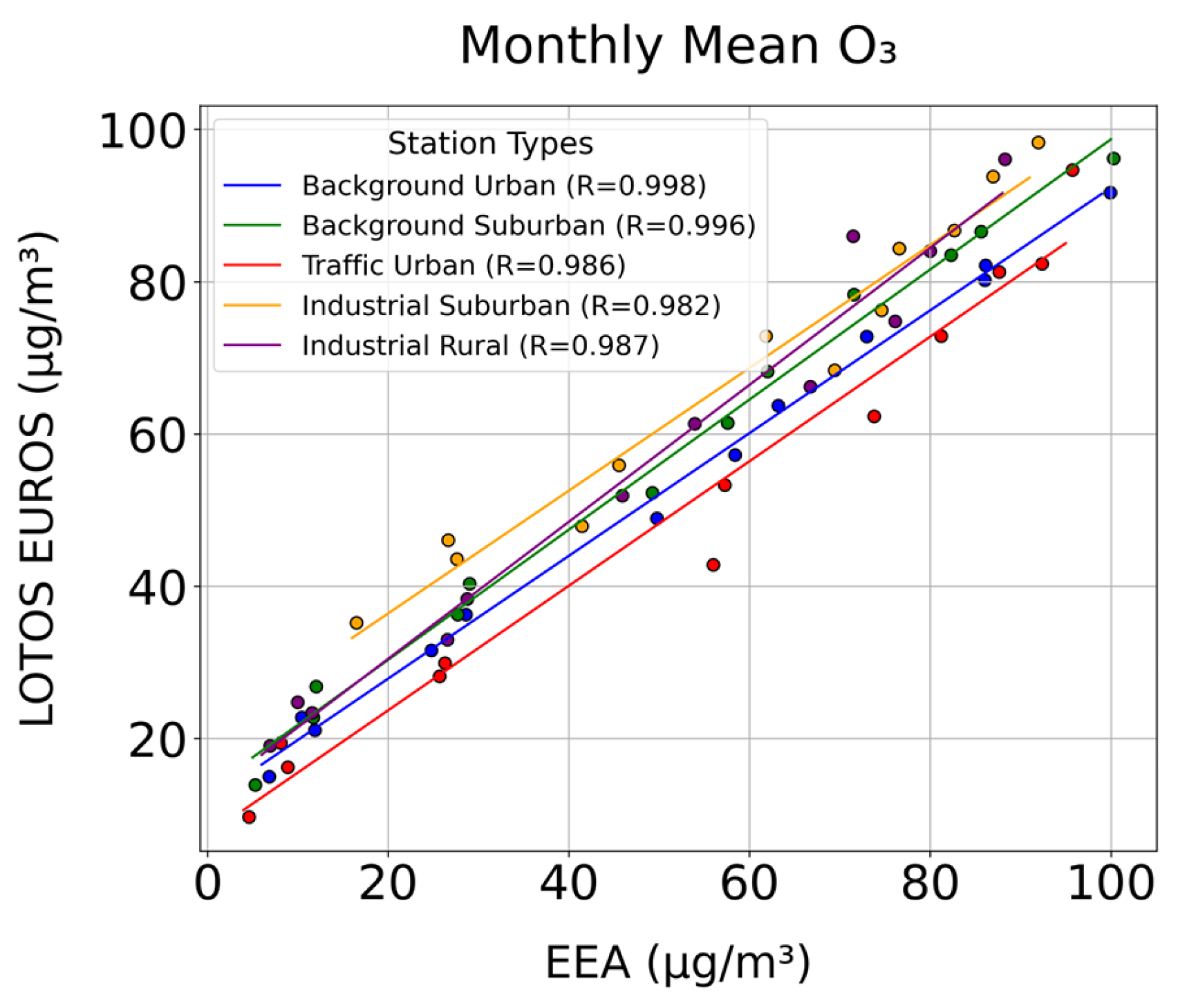
Figure 6.
Seasonal diurnal variability of EEA surface (a), (c) ozone and (b), (d) nitrogen dioxide concentrations (μg/m3) for one traffic urban and two industrial suburban stations over the Po Valley. The shaded areas represent the standard deviation of the hourly mean.
Figure 6.
Seasonal diurnal variability of EEA surface (a), (c) ozone and (b), (d) nitrogen dioxide concentrations (μg/m3) for one traffic urban and two industrial suburban stations over the Po Valley. The shaded areas represent the standard deviation of the hourly mean.
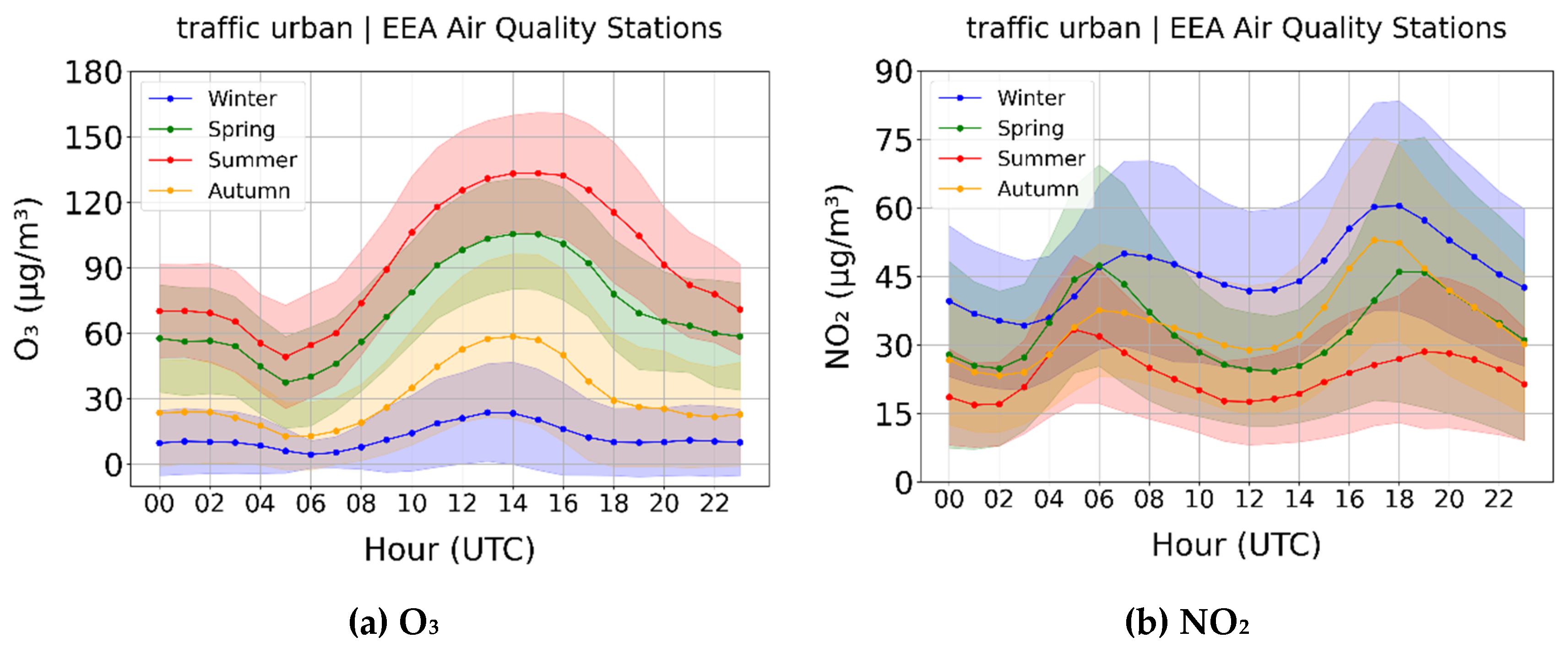
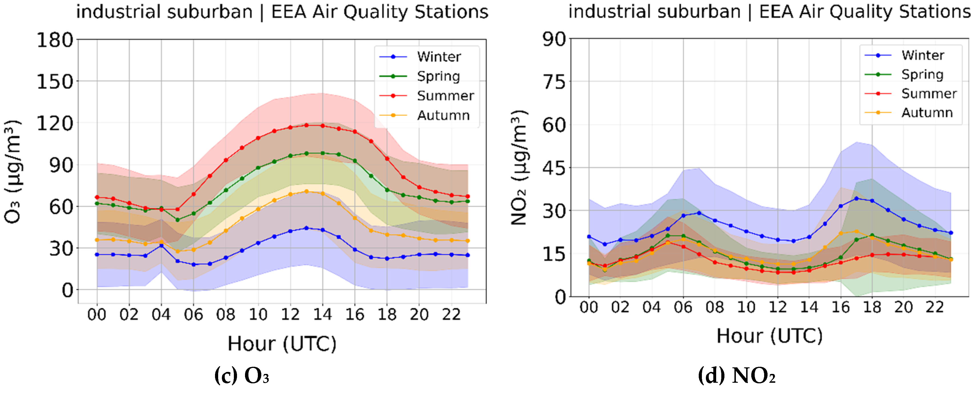
Figure 7.
Seasonal diurnal mean LOTOS-EUROS surface (a), (c) ozone and (b), (d) nitrogen dioxide concentration (μg/m3) for one traffic urban and two industrial suburban stations over the Po Valley.
Figure 7.
Seasonal diurnal mean LOTOS-EUROS surface (a), (c) ozone and (b), (d) nitrogen dioxide concentration (μg/m3) for one traffic urban and two industrial suburban stations over the Po Valley.
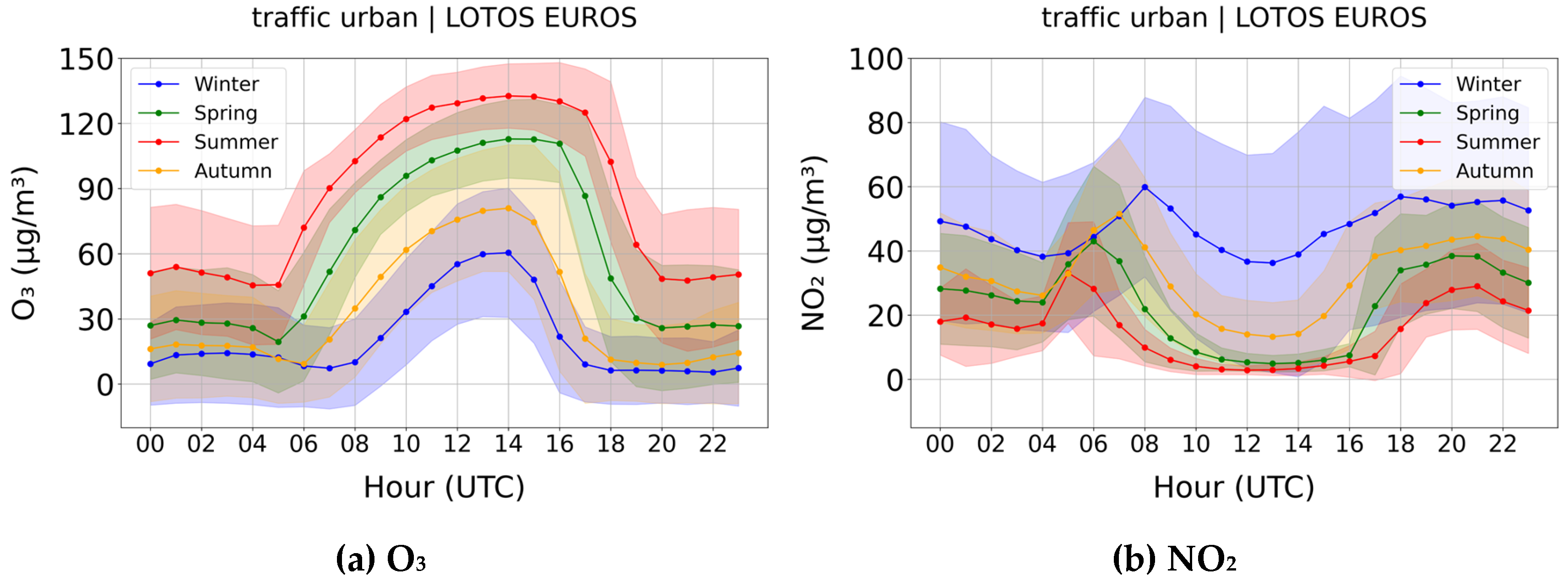
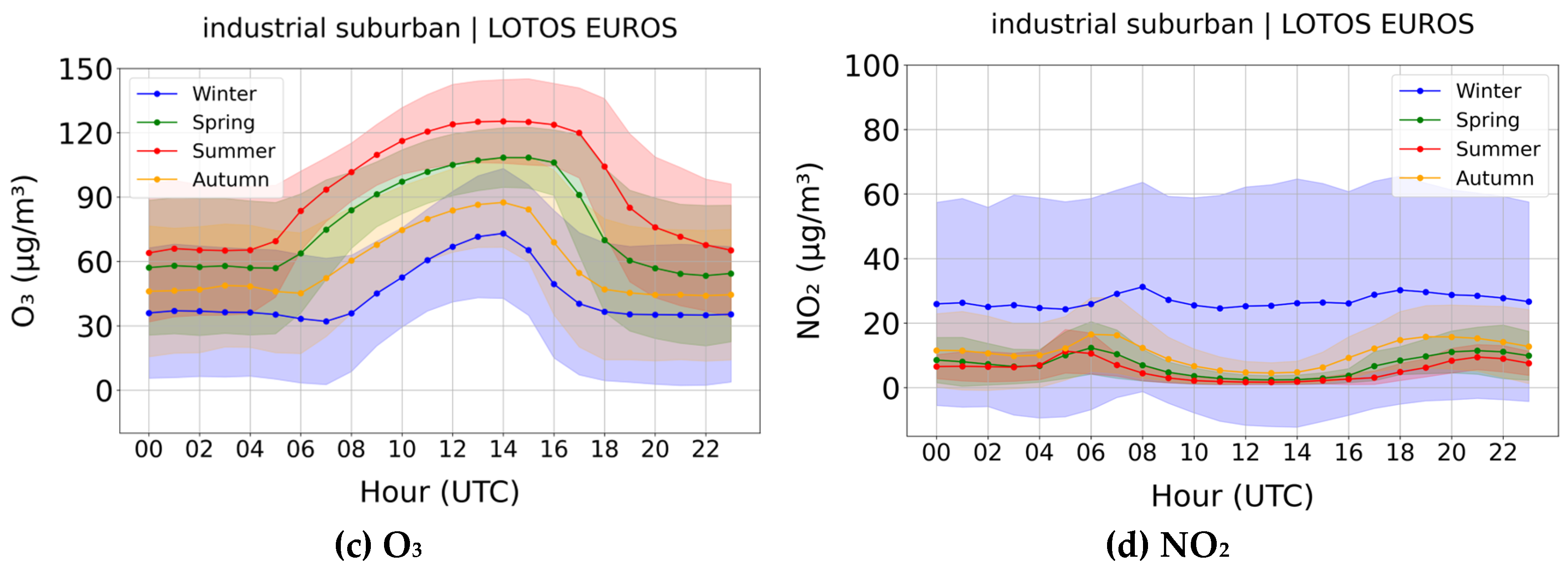
Figure 9.
Scatterplot of monthly mean surface ozone and nitrogen dioxide concentration (μg/m3) for all station types from (a) EEA stations and (b) LOTOS-EUROS simulations over the Po Valley.
Figure 9.
Scatterplot of monthly mean surface ozone and nitrogen dioxide concentration (μg/m3) for all station types from (a) EEA stations and (b) LOTOS-EUROS simulations over the Po Valley.
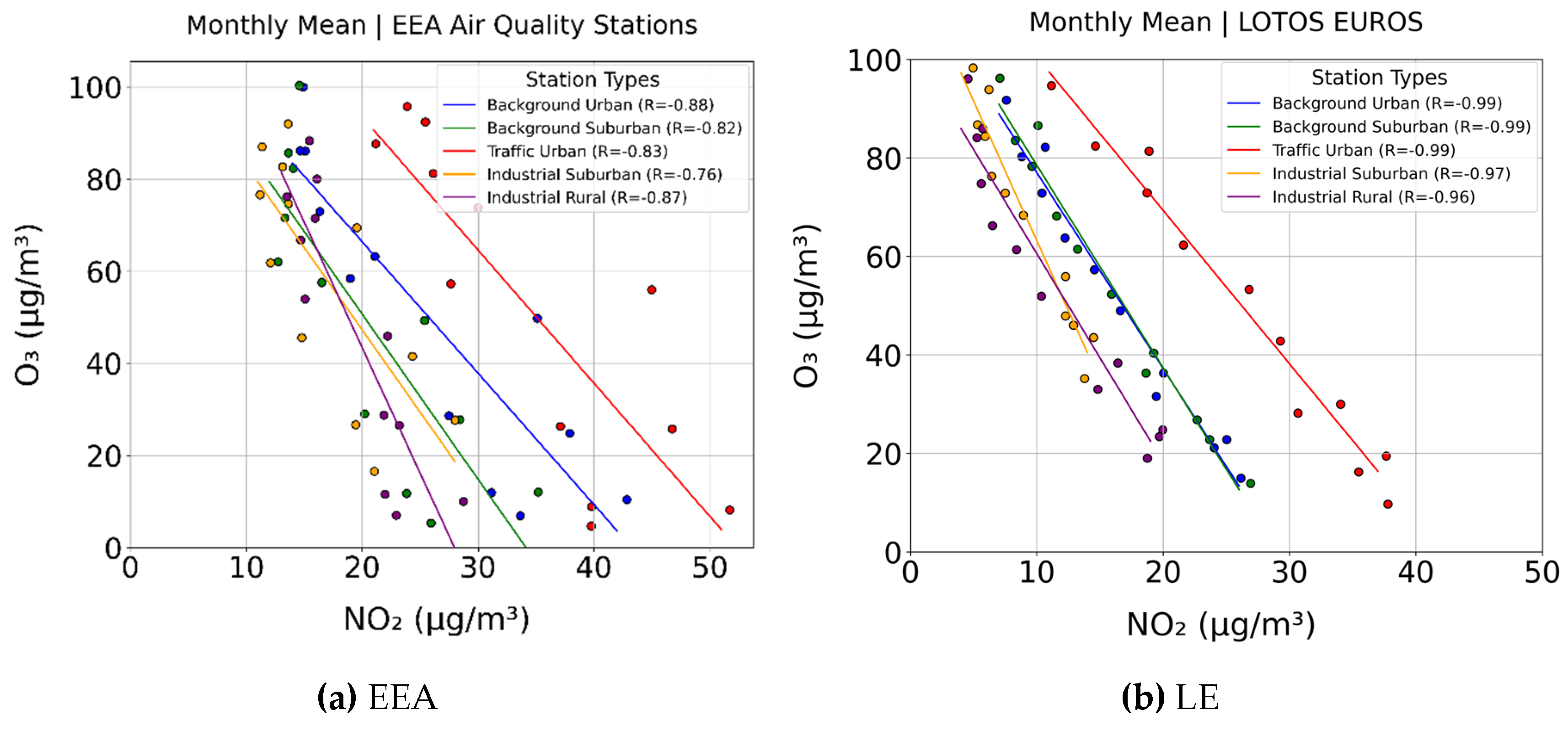
Figure 10.
Number of days exceeding the EU ozone 8h limit for the locations of EEA in situ stations as reported by the ground-based measurements (a) and the LOTOS-EUROS simulations (b).
Figure 10.
Number of days exceeding the EU ozone 8h limit for the locations of EEA in situ stations as reported by the ground-based measurements (a) and the LOTOS-EUROS simulations (b).
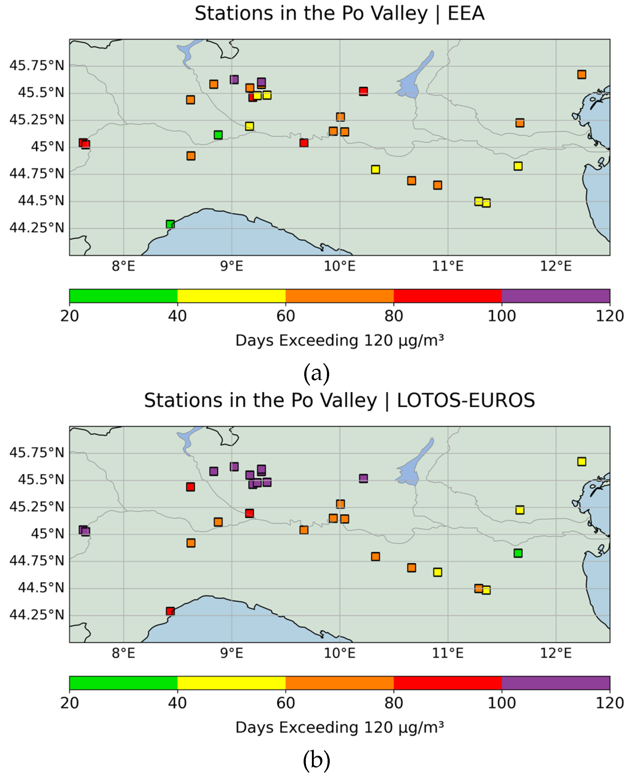
Table 1.
Annual mean O₃ and NO₂ concentrations (μg/m³) and the min & max monthly mean levels reported per different type of station.
Table 1.
Annual mean O₃ and NO₂ concentrations (μg/m³) and the min & max monthly mean levels reported per different type of station.
| Station Type | Annual O₃ | Monthly O₃ | Annual NO2 | Monthly NO2 | ||
|---|---|---|---|---|---|---|
| (mean ± 1σ) | max | min | (mean ± 1σ) | max | min | |
| Background urban | 49.90 ± 32.82 | 99.94 | 6.82 | 25.76 ± 10.14 | 42.84 | 14.65 |
| Background suburban | 49.52 ± 32.12 | 100.27 | 5.27 | 20.31 ± 7.35 | 35.18 | 12.74 |
| Traffic urban | 51.46 ± 35.11 | 95.72 | 4.61 | 34.53 ± 10.13 | 51.71 | 21.16 |
| Industrial suburban | 58.47 ± 25.97 | 91.96 | 16.50 | 16.85 ± 5.52 | 28.01 | 11.19 |
| Industrial rural | 47.18 ± 29.64 | 88.28 | 6.93 | 19.30 ± 4.76 | 28.73 | 13.50 |
Table 2.
Seasonal urban correlation coefficients for all types of stations (pvalue<< 0).
| R Value | |||||
|---|---|---|---|---|---|
| Station Type | Winter | Spring | Summer | Autumn | |
| Background urban | 0.98 | 0.96 | 0.94 | 0.97 | |
| Background suburban | 0.98 | 0.95 | 0.94 | 0.95 | |
| Traffic urban | 0.93 | 0.87 | 0.83 | 0.87 | |
| Industrial suburban | 0.93 | 0.95 | 0.98 | 0.97 | |
| Industrial rural | 0.94 | 0.96 | 0.96 | 0.97 | |
Disclaimer/Publisher’s Note: The statements, opinions and data contained in all publications are solely those of the individual author(s) and contributor(s) and not of MDPI and/or the editor(s). MDPI and/or the editor(s) disclaim responsibility for any injury to people or property resulting from any ideas, methods, instructions or products referred to in the content. |
© 2025 by the authors. Licensee MDPI, Basel, Switzerland. This article is an open access article distributed under the terms and conditions of the Creative Commons Attribution (CC BY) license (http://creativecommons.org/licenses/by/4.0/).
Copyright: This open access article is published under a Creative Commons CC BY 4.0 license, which permit the free download, distribution, and reuse, provided that the author and preprint are cited in any reuse.


