Submitted:
06 November 2025
Posted:
06 November 2025
You are already at the latest version
Abstract
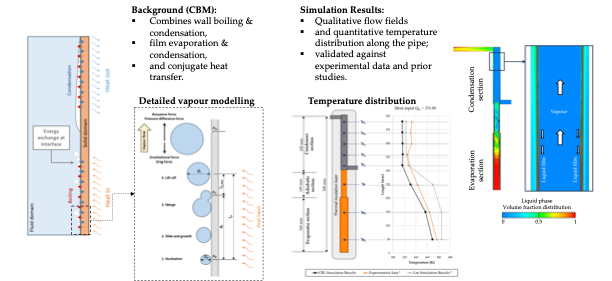
Predicting phase-change heat transfer in heat pipes represents a significant challenge owing to the complex interaction of boiling, condensation, and conjugate heat transfer mechanisms. This study presents a numerical investigation of a closed two-phase ther-mosyphon using the Combined Boiling Model (CBM) within a conjugate heat transfer (CHT) framework. The model combines wall boiling, film condensation, and bulk phase-change processes in an Euler–Euler multiphase formulation. Simulations were performed for heat loads ranging from 173 W to 376 W. The results were validated against experimental measurements and compared with predictions obtained using the VOF–Lee model. The CBM accurately reproduced key flow features, including vapour generation, vapour-pocket dynamics, and thin-film condensation, while reducing temperature de-viations typically below 3% in the evaporator and adiabatic sections and about 2 to 5% in the condenser. The results confirm that the CBM provides a physically consistent and computationally efficient approach for predicting evaporation–condensation phenomena in heat pipes.
Keywords:
heat pipe
; thermosyphon
; multiphase
; conjugate heat transfer
; Combined Boiling Model (CBM)
; Euler-Euler
1. Introduction
Cooling systems used in modern applications are becoming increasingly complex, reflecting the growing sophistication of the components they serve. Adequate and efficient heat dissipation is essential for ensuring the reliable operation of devices such as electric motors, hydrogen fuel cells, control units, and motherboards, batteries [1,2], particularly in industries like automotive and aerospace. As the demand for compact and powerful electronic systems rises, traditional single-phase cooling approaches are no longer sufficient. Instead, modern thermal management relies on processes that combine heat transfer with phase-change phenomena.
Among these, heat pipes have been studied extensively due to their ability to transfer large heat loads with minimal temperature gradients. First investigated in the 19th century [3] and formalized by Grover in 1963 [4], heat pipes exploit evaporation and condensation to achieve exceptionally high effective thermal conductivity. Predicting their thermal–fluid behaviour, however, is challenging due to the interplay of multiphase flow, compressibility, and conjugate heat transfer.
Early analytical models treated heat pipes as one-dimensional conduction systems with simplified assumptions for fluid transport [5], but modern studies increasingly employ computational fluid dynamics (CFD) to resolve vapour flow, liquid film dynamics, and interfacial phase change [6].
In its simplest form, a heat pipe is a closed thermosiphon as shown in Figure 1.
Despite their apparent simplicity as closed thermosiphons, accurate simulations must account for nucleate boiling, condensation, and evaporation processes. Operation in the nucleate boiling regime is desirable for high heat transfer, yet the narrow temperature window (e.g., ΔT ≈ 1–30 °C for water at atmospheric pressure) imposes strict modelling requirements [7,8].
Various CFD studies on subcooled wall boiling have been reported in the literature [9,10,11]. These reviews indicate that researchers primarily employ interfacial surface tracking methods, such as Volume-of-Fluid (VOF), or the Euler–Euler framework to model boiling phenomena. VOF enables detailed bubble- and droplet-scale studies but is computationally expensive [12,13,14,15] , whereas Euler–Euler, based on averaged field equations, allows for coarser grids and larger time steps, making it computationally more efficient and thus more suitable for practical engineering applications.
Within the latter, the widely used RPI wall-boiling model [16] often requires empirical recalibration and may under predict flow boiling [17,18,19,20]. Improvements are needed, particularly for heat pipes where circulation arises from combined pressure and gravity effects.
Evaporation and condensation models are also essential for capturing vapour transport, with Lee’s approach [13,21,22,23,24] showing strong agreement with experiments [8]. For realistic systems, conjugate heat transfer (CHT) between fluid and solid domains must be included, though only a few studies have addressed multiphase CHT comprehensively [11,25].
In previous work, we proposed the Combined Boiling Model (CBM) and validated it in a simplified CHT case [26]. Here, we extend its application to heat pipes, focusing on phase-change heat transfer under realistic operating conditions.
2. Model Description
2.1. Background
The CBM model was developed and preliminary validation on a simplified case employed in our previous study [26] . That case represented an open system with a velocity inlet and a pressure outlet boundary condition, consisting of two domains: the fluid region and a solid heating plate. A detailed grid-independence and time-step sensitivity analysis was performed, from which the optimal numerical parameters were established. These parameters were subsequently applied to the more complex heat pipe model investigated in the present work.
In contrast to the Robinson-type duct of the previous study, the present model represents a closed vertical heat pipe filled with working fluid. It comprises three main components: the fluid domain of the pipe, the solid copper casing, and the coolant region at the condenser side Figure 2.
Geometrically, this configuration is not significantly more complex than the Robinson test duct; however, from a numerical perspective it is considerably more challenging. In particular, the closed domain requires consideration of vapour compressibility. Furthermore, bubble dynamics are no longer dictated by inlet velocity, but instead result from buoyancy forces, pressure gradients, and bubble drag within the flow, all of which must be explicitly resolved.
In addition, heat pipe simulations must account for condensation processes. For this reason, a simplified film-condensation model has been incorporated into the CBM. The key extensions relative to the original analysis are summarized as follows:
- closed system,
- weakly compressible vapour flow,
- inclusion of condensation,
- three interacting domains: the solid domain (single-phase, energy equation), the heat pipe fluid domain (multiphase), and the coolant domain (single-phase flow).
2.2. Governing Equations
The Euler–Euler multi-fluid framework treats each phase as an interpenetrating continuum, with interphase exchange terms added to the conservation laws [27]. Ensemble averaging removes microscopic interfaces and yields macroscopic equations analogous to single-phase flow, extended by phase volume fractions and interfacial transfer terms [28,29,30]. Based on the formulation of Drew and Passman [31], the governing equations are:
Continuity equation (phase k):
with the compatibility condition
Momentum equation (phasek):
where f includes gravity and inertial forces. Pressure is assumed equal for all phases:
2.3. Interfacial Momentum Exchange
The interfacial momentum source term accounts for drag, turbulent dispersion, lift, and wall lubrication:
The drag contribution is given by
where vr = vd - vc.
In AVL FIRE™, the latest Gas-Liquid System 3 [27,32] is used. It blends bubbly and droplet drag correlations based on dispersed-phase volume fraction, using Schiller–Naumann [33] or Tomiyama [34] models depending on bubble size and Eötvös number. Turbulent dispersion accounts for vapour diffusion in mixing flows.
2.4. Wall Boiling Model
The near-wall heat transfer is modelled using the RPI framework of Kurul and Podowski [16], extended for forced convective boiling following Gilman [19], with further simplifications by Shi and Zhang [20]. The complete formulation, including detailed derivations, was presented in our previous work [26], therefore only the governing partitioning and key correlations will be presented in this section .
The total wall heat flux is expressed as:
The evaporative component is:
with bubble departure frequency f [35], nucleation site density Nw [36], and departure diameter Dl [37] obtained from standard correlations.
The convective contribution is:
Stationary and sliding bubble quenching fluxes are:
where hquen is the transient conduction coefficient [38].
The sliding bubble model accounts for bubble nucleation, growth, sliding, merging, and eventual lift-off along the heated wall (Figure 3).
Bubble motion is governed by the balance of buoyancy, pressure-difference, gravitational, and drag forces. Nucleated bubbles first grow and slide along the wall, during which they exchange heat with the liquid and contribute to the sliding heat flux. As they move, bubbles may coalesce with neighbouring bubbles at a distance defined by the nucleation site spacing gs, leading to accelerated growth. The sliding distance lsl therefore depends on the number of merged bubbles nnr and the remaining distance before lift-off [19,20].
Lift-off occurs once the bubble reaches the departure diameter Dl, determined by buoyancy–drag balance and surface tension constraints. The corresponding sliding velocity is obtained iteratively since the drag coefficient Cd depends on the bubble Reynolds number. In this way, the model explicitly captures the four key stages of bubble dynamics: (1) nucleation, (2) sliding and growth, (3) coalescence, and (4) lift-off.
2.5. Film Condensation Model
A simplified film condensation model based on Nusselt theory for laminar condensation on vertical walls [39] was applied in the present investigation. The model assumes: Tw < Tsat, a liquid film is always present, liquid velocity is negligible, and all wall heat flux is converted into condensation.
The film thickness is approximated as:
where αl is the liquid volume fraction, VP is the cell volume, and Ab is the cell wall area exposed to condensation.
The temperature gradient across the film is:
The wall heat flux is:
where kl is the liquid thermal conductivity.
The corresponding cell condensation rate is:
where hfg is the latent heat of vaporization.
2.6. Flow Evaporation and Condensation
2.7. Fluid–Solid Conjugate Heat Transfer
Conjugate heat transfer (CHT) between solid and fluid domains is modelled using an interfacial diffusion coefficient. The coefficient is derived from the heat flux , obtained from the modified RPI model, and the interface temperature difference :
where A is the heated surface area and cp,l the liquid specific heat capacity.
The computed diffusion coefficient is assigned to the fluid domain to evaluate the local heat transfer coefficient. This is then imposed as a boundary condition on the solid domain, where the wall temperature Tw is recalculated. The updated Tw is in turn enforced at the fluid side, ensuring coupled exchange. The process is repeated iteratively within each time step until thermal equilibrium is achieved.
3. Computational Model
The updated Combined Boiling Model (CBM) simulations were compared against experimental data reported by Fadhl, Wrobel, and Jouhara [12] and detailed in Fadhl’s dissertation [8]. The dataset provides thermal conditions in a closed thermosyphon at various power inputs; in the present study, two representative operating conditions were selected. The experimental setup is shown schematically in Figure 4.
Eight thermocouples were mounted along the outer wall of the heat pipe, with measurement positions distributed from the condenser to the evaporator section.
3.1. Computational Mesh and Time-Step
Based on the test rig geometry, a multi-domain block-structured mesh was created, comprising 161.280 cells (Figure 5).
The fluid domain contained 56.000 cells (blue), the solid copper domain 59,200 cells (orange), and the coolant domain 46.080 cells (grey).
A full mesh/time-step sensitivity study was not repeated here, as this was performed in earlier work [26]. That study showed that meshes finer than 1 mm adequately resolved vapour distribution, with interface temperature deviations within ±5 percentage of experiments. Wall resolution yielded low y+ values (8–20), which, although below the values often suggested for Euler–Euler boiling simulations (y+ > 40 [43]), ensured consistent temperature prediction. A 1.0 mm mesh with Δt = 0.005 s was identified as the optimal configuration.
In the present work, these settings were adopted with additional near-wall refinement (0.4 mm boundary layer and five solid layers of 0.18 mm each) to capture condensation films without artificial breakup in the Euler–Euler framework.
3.2. Numerical Settings
All simulations were performed in transient mode using the Euler–Euler framework with the models described above. Three computational domains were considered: fluid, solid, and coolant. In the solid domain, only the energy equation was solved, while the fluid domain included continuity, momentum, turbulence, energy, and volume fraction equations. The Combined Boiling Model (CBM) was applied to capture near-wall phase change. Key simulation parameters for the multiphase fluid domain are summarized in Table 1.
The interfacial exchange models (Table 2) employed the CBM for mass and energy transfer, “Gas–Liquid System 3” for momentum exchange, Tomiyama’s correlation for bubbles (1 mm) and Schiller–Naumann for droplets (0.5 mm).
A sensitivity study on bubble and droplet departure parameters, was not conducted in present study those the default values provided by AVL FIRE™ were retained.
Water properties were taken from the software database; vapour was modelled as a weakly compressible ideal gas. Phase change was restricted to the saturation temperature, with vapour pressure following the standard saturation curve (Figure 6).
Solver stability and accuracy were maintained using the SIMPLE algorithm for pressure–velocity coupling. Convergence criteria were set to 1 × 10⁻⁴ for continuity, energy, and volume fraction, and 5 × 10⁻⁴ for momentum and turbulence. The MINMOD differencing scheme with 40% upwind blending [44] was used on momentum, volume fraction and energy. Using these settings, the number of iterations fluctuated between 5 and 20 per time step, with higher values occurring during boiling or condensation onset.
3.3. Initial and Boundary Conditions
Boundary conditions were specified for all three computational domains. In the condenser heat exchanger domain, a water inlet mass flow rate of 0.003 kg/s at 293.75 K was imposed, while the outlet was set to ambient pressure (Figure 5). The external walls were treated as adiabatic. The solid domain was defined as copper, and a prescribed heat rate boundary condition was applied at the evaporator section (Figure 5). Two heat load cases were investigated, 173 W and 376 W. The heat pipe fluid domain was initialized with a mixture of liquid water and water vapour, with the evaporator section fully filled with liquid water, corresponding to a filling ratio of 1, and the upper region filled with water vapour.
4. Results and Discussion
4.1. Initial Flow Simulation
The simulations were conducted in two stages. In the first stage, the coolant flow field was solved until a quasi-steady state was reached. This solution was subsequently used to initialize the full conjugate heat transfer (CHT) model, thereby ensuring a physically consistent start-up condition for the coupled phase-change simulation.
The computed coolant velocity field is illustrated in Figure 7 (a), where the colour contours represent the velocity magnitude and the streamlines indicate the flow direction. The coolant flow simulation was performed for a total duration of 60 s; however, a quasi-steady state was reached after approximately 30 s, as confirmed by the outlet mass flow rate presented in Figure 7 (b).
This preliminary step provided a stable and realistic hydrodynamic field for the subsequent CHT simulations, minimizing numerical transients during model initialization.
4.2. CHT Full-Model Simulation
In current preliminary validation study five CHT simulations were performed and analysed, of which three were compared directly with available experimental and numerical data [12]. The coupled vapour–liquid flow dynamics developed primarily during the initial transient period, while the overall thermal response required a longer time to stabilize.
The transient development of the liquid and vapour phases is best observed for the 100% filling ratio, in which the entire evaporator section was initially filled with liquid water, and the remaining adiabatic and condenser sections contained pure vapour. The evolution of the liquid volume fraction for two representative heat loads (173 W and 376 W) is shown in Figure 8.
At the beginning of the simulation, a rapid evaporation rate was observed in both cases, stabilizing after approximately 10 s. The larger vapour generation at higher heat input (376 W) became evident after this period. The formation of large vapour pockets was observed in the adiabatic section before collapsing into the condenser region. Within the condenser, the simulations consistently predicted the formation of a thin liquid film on the upper wall surface, as illustrated in Figure 9.
The fluid flow in this region clearly show vapour transport toward the upper condensation surface, followed by flow reversal and downward liquid-film drainage. This behaviour is consistent with experimental observations and confirms that the present model is capable of capturing the essential evaporation–condensation mechanisms occurring within the heat pipe.
4.3. Preliminary Model Validation
Experimental validation data were available for a 50% fill ratio [8], corresponding to half of the evaporator section being initially filled with liquid water , while the remaining volume contained vapour. Three heat-input cases were investigated: 173 W, 225 W, and 376 W.
Due to the low amount of liquid phase, the closed thermosyphon exhibited slightly different behaviour compared to the 100% fill-ratio case discussed earlier. The flow evolution during the initial transient period for the two representative heat inputs (173 W and 376 W) is illustrated in Figure 10.
At start-up (up to approximately 8 s), both cases showed similar evaporation patterns within the evaporator section. However, after a longer time (approximately 30 s), the 376 W case displayed significantly less residual liquid in the evaporator section and a noticeably thicker condensate film in the condenser section. The stronger evaporation and higher vapour production observed at 376 W are consistent with the expected temperature increase under higher thermal loading. The influence of heat input on the overall temperature distribution is shown in Figure 11.
The temperature gradients within the heat pipe are clearly visible, with the highest temperatures occurring in the evaporator section at 376 W. A slight flow asymmetry was observed, resulting from the lower position of the coolant inlet. The colder coolant entered from the bottom, absorbed heat as it travelled through the condenser, and gradually increased in temperature before exiting from the opposite upper side.
Quantitative comparisons further support the validity of the proposed CBM (Combined Boiling Model) approach. The results show improved agreement with experimental measurements and with previous numerical studies using the VOF–Lee model [8]. Temperatures were monitored at eight locations, as shown in Figure 4, and the computed values were compared with both experimental data and Lee model predictions.
4.3.1. Heat Input: 173 W
At 173 W, deviations in the condenser remained below 3.5%, despite the use of a simplified condensation model. The largest improvement compared to the Lee results occurred in the evaporator, where deviations were reduced to 1.27% and 1.79%, compared with 9.42% and 12.14% in the previous model. In the adiabatic section, the deviation decreased from 10.68% (Lee) to 3.13% (CBM).
4.3.2. Heat Input: 225 W
At 225 W, the Lee model achieved slightly better agreement in the condenser (errors typically below 1%), whereas the CBM model exhibited deviations between 2–4% in this region. However, the CBM model significantly outperformed the Lee model in the evaporator and adiabatic sections, where deviations were reduced to 2.30%, 1.66%, and 3.38%, compared with 2.72%, 10.49%, and 10.32% for the Lee model.
4.3.3. Heat Input: 376 W
4.4. Overall Model Performance
The overall performance of the model, together with its comparison against experimental data and the Lee model results, is presented in Figure 12. Although detailed deviations from the experimental measurements were provided in the previous tables, the overall agreement can be more clearly visualized by examining the trend line curves. The markers in the figure correspond to the individual measurement points, while the solid lines represent the fitted trend lines. From these results, it can be concluded that the proposed Combined Boiling Model (CBM) provides a markedly improved prediction of the thermal behaviour of the analysed heat pipe across all investigated heat loads.
While the condensation sub-model integrated within the CBM framework remains simplified, the achieved level of agreement with experimental data indicates that the CBM approach successfully captures the dominant physical mechanisms governing evaporation–condensation interactions. Further refinement of the condensation treatment is expected to reduce residual deviations, particularly under varying thermal loads and transient operating conditions.
In summary, the proposed model demonstrates robust predictive capability for coupled phase-change dynamics in heat pipes and provides a solid foundation for the future development of high-fidelity, physics-based phase-change models in CFD.
5. Conclusions
A comprehensive numerical investigation of a closed two-phase thermosyphon (basic heat pipe) was performed using the Combined Boiling Model (CBM) [26] within a conjugate heat transfer (CHT) framework. The study focused on the preliminary validation of the model against experimental data and previously published numerical results for different heat loads ranging from 173 W to 376 W. The main conclusions can be summarized as follows:
- Numerical stability and initialization:
The two-stage simulation strategy—first solving for steady coolant flow and then initializing the CHT model—provided a stable and physically consistent start-up condition, reducing numerical transients and improving convergence of the coupled phase-change solution.
- Prediction of flow and phase distribution:
The CBM model successfully reproduced the key flow features of the thermosyphon, including vapour generation in the evaporator, vapour-pocket formation and subsequent collapse in the adiabatic section, and thin-film condensation along the upper condenser wall. The predicted flow reversal and liquid-film drainage showed strong agreement with theoretical expectations and experimental observations, confirming that the model accurately reproduces the essential evaporation–condensation mechanisms.
- Validation against experimental data:
Across all investigated heat loads, the CBM model shows close agreement with measurements, with the strongest accuracy in the evaporator and adiabatic regions. Compared with a traditional VOF-Lee formulation, temperature deviations are markedly lower, in some cases by up to an order of magnitude, which highlights the improved predictive performance of the proposed approach. A key practical advantage is efficiency: CBM attains these results with time steps about ten times larger and with coarser meshes than VOF Lee, which leads to substantially shorter runtimes. The two approaches however target different use cases. CBM is well suited for fast, system scale simulations of engineering devices where overall thermal behaviour is the priority, whereas VOF-Lee remains preferable for interface resolved, microscale phenomena such as geyser boiling where an explicitly captured vapour liquid interface is required.
- Influence of fill ratio and heat load:
The simulations accurately captured the sensitivity of thermosyphon operation to the initial liquid inventory. Higher heat inputs led to stronger evaporation, larger vapour volumes, and thicker condensate films, consistent with experimental trends.
- Model limitations and future work:
While the current condensation sub-model remains simplified, the achieved level of accuracy indicates that the CBM framework effectively captures the dominant heat and mass transfer mechanisms. The present work represents only a preliminary validation study and a demonstration of the feasibility of applying the CBM model to heat pipe simulations. Further, more extensive validation under a wider range of operating conditions and with various working fluids is required to extend the model’s applicability and reliability.
These findings highlight the potential of the CBM framework as a reliable and computationally efficient tool for modelling two-phase heat transfer in advanced thermal management systems. This represents the best agreement with experimental data currently reported in the literature for such simulations problems.
Author Contributions
Conceptualization, J.S. and M.Z.; methodology, J.S. and M.Z.; software, J.S.; validation, J.S.; formal analysis, J.S.; investigation, J.S.; resources, J.S. and M.Z.; data curation, J.S. and M.Z.; writing—original draft preparation, J.S., M.Z. and J.M.; writing—review and editing, J.S., M.Z. and J.M; visualization, J.S.; supervision, M.Z. and J.M.; project administration, M.Z.; funding acquisition, M.Z. and J.M. All authors have read and agreed to the published version of the manuscript.
Funding
This research received no external funding
Data Availability Statement
Data are available on reasonable request from the corresponding author. Portions of the dataset are subject to third-party intellectual-property and confidentiality obligations and cannot be disclosed. Only materials cleared for release (non-confidential and non-proprietary) can be shared.
Acknowledgments
The study was undertaken under the guidance and support of the Faculty of Mechanical Engineering, University of Maribor (Chair of Power, Process, and Environmental Engineering). The authors further acknowledge the technical support of AVL-AST d.o.o.
Conflicts of Interest
The authors declare no conflicts of interest.
Abbreviations
The following abbreviations are used in this manuscript:
| CBM | Combined Boiling Model |
| CHT | Conjugate Heat Transfer |
| CFD | Computational Fluid Dynamics |
| VOF | Volume of Fluid |
| RPI | (Kurul–Podowski) wall-boiling model, commonly called the RPI model |
| SIMPLE | Semi-Implicit Method for Pressure-Linked Equations (pressure–velocity coupling) |
| k–ε–ζ–f | Turbulence model (k-epsilon-zeta-f) |
| y+ | Dimensionless wall distance (near-wall mesh metric) |
References
- Zhao, C.; Zhang, B.; Zheng, Y.; Huang, S.; Yan, T.; Liu, X. Hybrid Battery Thermal Management System in Electrical Vehicles: A Review. Energies 2020, 13, 6257. [Google Scholar] [CrossRef]
- Wang, X.; Liu, S.; Zhang, Y.; Lv, S.; Ni, H.; Deng, Y.; Yuan, Y. A Review of the Power Battery Thermal Management System with Different Cooling, Heating and Coupling System. Energies 2022, 15, 1963. [Google Scholar] [CrossRef]
- D. A. Reay, P. A. Kew, and R. McGlen, Heat Pipes : Theory, Design and Applications. Oxford: Butterworth-Heinemann (in English), 2013.
- G. M. Grover, "Evaporation-condensation heat transfer device," ed:. Google Patents 1966.
- J. G. Collier and J. R. Thome, "Convective boiling and condensation - Third edition," ed. Switzerland, Europe: Oxford University Press (Oxford), 1994.
- Kharangate, C.R.; Mudawar, I. Review of computational studies on boiling and condensation. Int. J. Heat Mass Transf. 2017, 108, 1164–1196. [Google Scholar] [CrossRef]
- T. L. Bergman, A. Lavine, F. P. Incropera, and D. P. DeWitt, Fundamentals of heat and mass transfer, 7th ed. ed. John Wiley & Sons (in English), 2011.
- B. Fadhl, "Modelling of the thermal behaviour of a two-phase closed thermosyphon," Ph.D., Brunel University (United Kingdom), 2016.
- Petersen, K.; Rahbarimanesh, S.; Brinkerhoff, J. Progress in physical modelling and numerical simulation of phase transitions in cryogenic pool boiling and cavitation. Appl. Math. Model. 2022, 116, 327–349. [Google Scholar] [CrossRef]
- Devahdhanush, V.; Lei, Y.; Chen, Z.; Mudawar, I. Assessing advantages and disadvantages of macro- and micro-channel flow boiling for high-heat-flux thermal management using computational and theoretical/empirical methods. Int. J. Heat Mass Transf. 2021, 169. [Google Scholar] [CrossRef]
- Han, J.; He, W.; Liu, Y.; Gao, D.; Zhao, C.; Bo, H. Numerical investigation of flow boiling characteristics in narrow rectangular channels using two-fluid Eulerian CFD model covering a wide range of pressures. Appl. Therm. Eng. 2024, 255. [Google Scholar] [CrossRef]
- Fadhl, B.; Wrobel, L.C. and Jouhara, H. Numerical modeling of the temperature distribution in a two-phase closed ther-mosyphon. Appl. Therm. Eng. 2013, 60, 122–131. [Google Scholar] [CrossRef]
- Wang, Z.; Turan, A.; Craft, T. Numerical Investigation of the Two-Phase Closed Thermosyphon Operating with Non-Uniform Heat Flux Profiles. Energies 2023, 16, 5141. [Google Scholar] [CrossRef]
- Edelbauer, W. Numerical simulation of cavitating injector flow and liquid spray break-up by combination of Eulerian–Eulerian and Volume-of-Fluid methods. Comput. Fluids 2017, 144, 19–33. [Google Scholar] [CrossRef]
- Edelbauer, W.; Birkhold, F.; Rankel, T.; Pavlović, Z.; Kolar, P. Simulation of the liquid break-up at an AdBlue injector with the volume-of-fluid method followed by off-line coupled Lagrangian particle tracking. Comput. Fluids 2017, 157, 294–311. [Google Scholar] [CrossRef]
- Kurul, N.; Podowski, M.Z. "Multidimensional effects in force convection subcooled boiling," in: Proceedings of the Ninth International Heat Transfer Conference, Jerusalem, Israel, 1990, pp. 21-26.
- Setoodeh, H.; Ding, W.; Lucas, D.; Hampel, U. Modelling and simulation of flow boiling with an Eulerian-Eulerian approach and integrated models for bubble dynamics and temperature-dependent heat partitioning. Int. J. Therm. Sci. 2021, 161, 106709. [Google Scholar] [CrossRef]
- Vlček, D.; Sato, Y. Sensitivity analysis for subcooled flow boiling using Eulerian CFD approach. Nucl. Eng. Des. 2023, 405, 112194. [Google Scholar] [CrossRef]
- L. A. Gilman, "Development of a General Purpose Subgrid Wall Boiling Model from Improved Physical Understanding for Use in Computational Fluid Dynamics," Ph.D., Department of Nuclear Science and Engineering, Massachusetts Institute of Technology, USA: Massachusetts, 2014.
- Shi, J.; Zhang, R.; Zhu, Z.; Ren, T.; Yan, C. A modified wall boiling model considering sliding bubbles based on the RPI wall boiling model. Int. J. Heat Mass Transf. 2020, 154, 119776. [Google Scholar] [CrossRef]
- Jouhara, H.; Fadhl, B.; Wrobel, L.C. Three-dimensional CFD simulation of geyser boiling in a two-phase closed thermosyphon. Int. J. Hydrogen Energy 2016, 41, 16463–16476. [Google Scholar] [CrossRef]
- Sadeghi, K.; Kahani, M.; Ahmadi, M.H.; Zamen, M. CFD Modelling and Visual Analysis of Heat Transfer and Flow Pattern in a Vertical Two-Phase Closed Thermosyphon for Moderate-Temperature Application. Energies 2022, 15, 8955. [Google Scholar] [CrossRef]
- Yang, D.; Bu, Z.; Jiao, B.; Wang, B.; Gan, Z. Numerical Study of Heat Transfer and Fluid Flow Characteristics of a Hydrogen Pulsating Heat Pipe with Medium Filling Ratio. Energies 2024, 17, 2697. [Google Scholar] [CrossRef]
- Cheng, Y.; Yu, H.; Zhang, Y.; Zhang, S.; Shi, Z.; Xie, J.; Zhang, S.; Liu, C. Heat Transfer Mechanism Study of an Embedded Heat Pipe for New Energy Consumption System Enhancement. Energies 2024, 17, 6162. [Google Scholar] [CrossRef]
- Godino, D.M.; Corzo, S.F.; Ramajo, D.E. CFD simulation of conjugated heat transfer with full boiling in OpenFOAM(R). Appl. Therm. Eng. 2022, 213, 118627. [Google Scholar] [CrossRef]
- Štrucl, J.; Marn, J.; Zadravec, M. Numerical modelling of conjugate heat transfer in force convective flow environment using a combined boiling model (CBM). Results Eng. 2025, 26. [Google Scholar] [CrossRef]
- FIRE, A. Version v2018, User's Manual. Graz, 2018.
- Greif, D.; Strucl, J. Numerical Study of Transient Multi Component Fuel Injection. SAE International Journal of Passenger Cars - Mechanical Systems, vol. 2013, p. 2550. [Google Scholar] [CrossRef]
- M. Ishii, "Thermo-fluid dynamic theory of two-phase flow," NASA STI/Recon Technical Report A, vol. 75, p. 29657, , 1975 1975. 01 January.
- R. T. Lahey and D. A. Drew, "AN ANALYSIS OF TWO-PHASE FLOW AND HEAT TRANSFER USING A MULTIDIMENSIONAL, MULTI-FIELD, TWO-FLUID COMPUTATIONAL FLUID DYNAMICS (CFD) MODEL," 2000.
- D. A. Drew and S. L. Passman, "Theory of Multicomponent Fluids," 1998.
- S. Mimouni, R. S. Mimouni, R. Denèfle, S. Gouénard - Fleau, and S. Vincent, "Multifield Approach and Interface Locating Method for Two-Phase Flows in Nuclear Power Plant," 2016, pp. 483-500.
- L. Schiller and Z. Naumann, "Über die Grundlegenden Berechnungen bei der Schwerkraftaufbereitung," Z.~Ver.~Dtsch.~Ing., vol. 77, pp. 318-320, 01/01 1933.
- Tomiyama, A.; Kataoka, I.; Zun, I.; Sakaguchi, T. Drag Coefficients of Single Bubbles under Normal and Micro Gravity Conditions. JSME Int. J. Ser. B 1998, 41, 472–479. [Google Scholar] [CrossRef]
- Cole, R. A photographic study of pool boiling in the region of the critical heat flux. AIChE J. 1960, 6, 533–538. [Google Scholar] [CrossRef]
- M. Lemmert and L. M. Chawla, "Influence of flow velocity on surface boiling heat transfer coefficient in Heat Transfer Boiling," E. Hahne and U. Grigull, Eds., ed. New York: Academic Press and Hemisphere, 1977, pp. 237-247.
- Tolubinski, V.I.; Kostanchuk, D.M. Vapour bubbles growth rate and heat transfer intensity at subcooled water boiling. In Proceedings of the 4th International Heat Transfer Conference, Paris-Versailles, France; 1970; pp. 1–11. [Google Scholar]
- Basu, N.; Warrier, G.R.; Dhir, V.K. Wall Heat Flux Partitioning During Subcooled Flow Boiling: Part 1—Model Development. J. Heat Transf. 2005, 127, 131–140. [Google Scholar] [CrossRef]
- W. Nusselt, Die Oberflächenkondensation des Wasserdampfes. VDI, 1916.
- W. H. Lee, PRESSURE ITERATION SCHEME FOR TWO-PHASE FLOW MODELING. 1980, pp. 407-431.
- Wu, H.; Peng, X.; Ye, P.; Gong, Y.E. Simulation of refrigerant flow boiling in serpentine tubes. Int. J. Heat Mass Transf. 2007, 50, 1186–1195. [Google Scholar] [CrossRef]
- De Schepper, S.C.; Heynderickx, G.J.; Marin, G.B. Modeling the evaporation of a hydrocarbon feedstock in the convection section of a steam cracker. Comput. Chem. Eng. 2009, 33, 122–132. [Google Scholar] [CrossRef]
- Vadlamudi, S.R.G.; Nayak, A.K. CFD simulation of Departure from Nucleate Boiling in vertical tubes under high pressure and high flow conditions. Nucl. Eng. Des. 2019, 352. [Google Scholar] [CrossRef]
- Sweby, P.K. High Resolution Schemes Using Flux Limiters for Hyperbolic Conservation Laws. SIAM J. Numer. Anal. 1984, 21, 995–1011. [Google Scholar] [CrossRef]
Figure 1.
Schematic of the complete thermosiphon cycle.
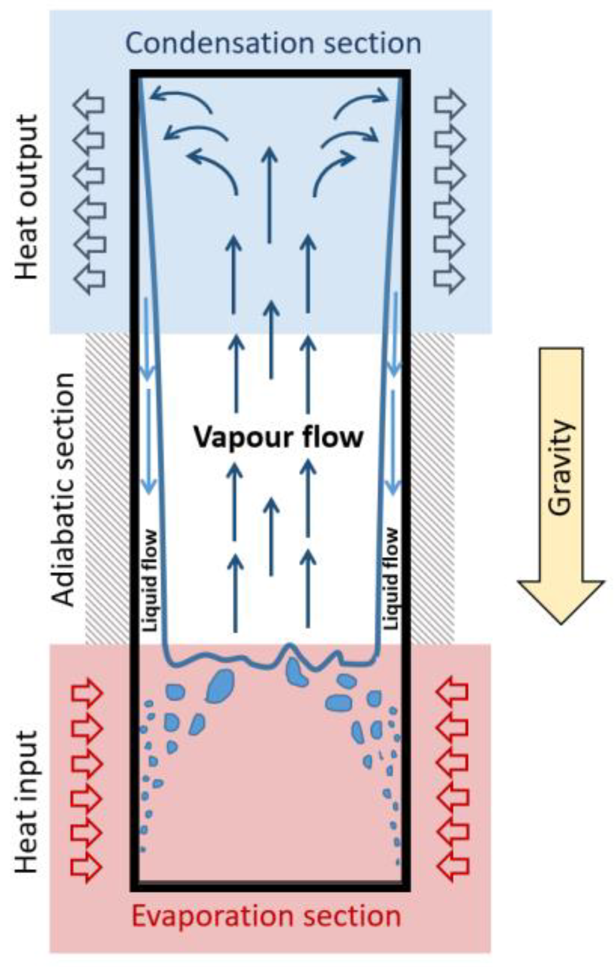
Figure 2.
Model components (computational domains).
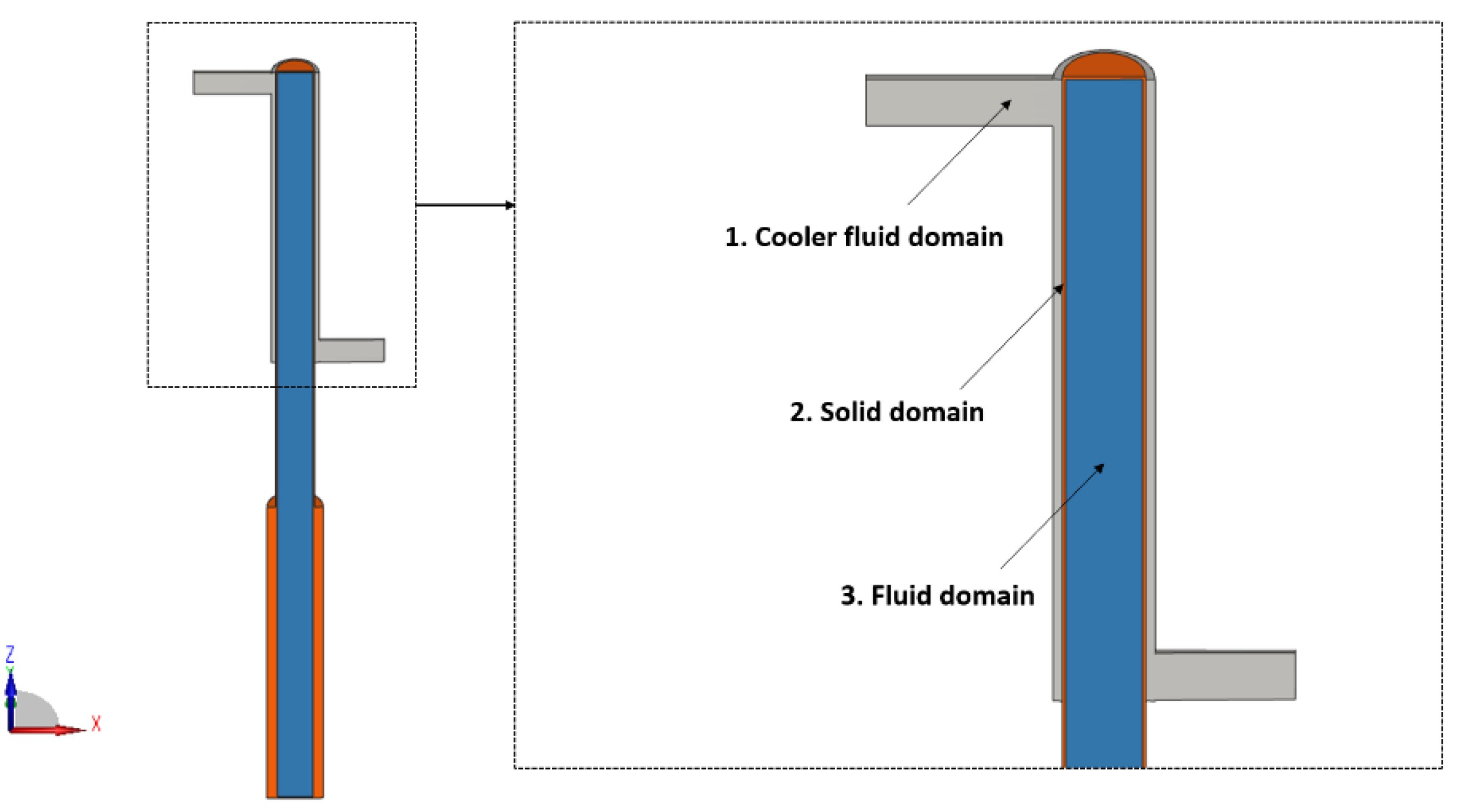
Figure 3.
Sliding bubble.
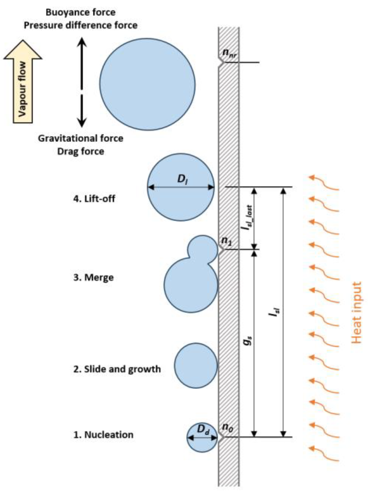
Figure 4.
Schematic representation of test rig.
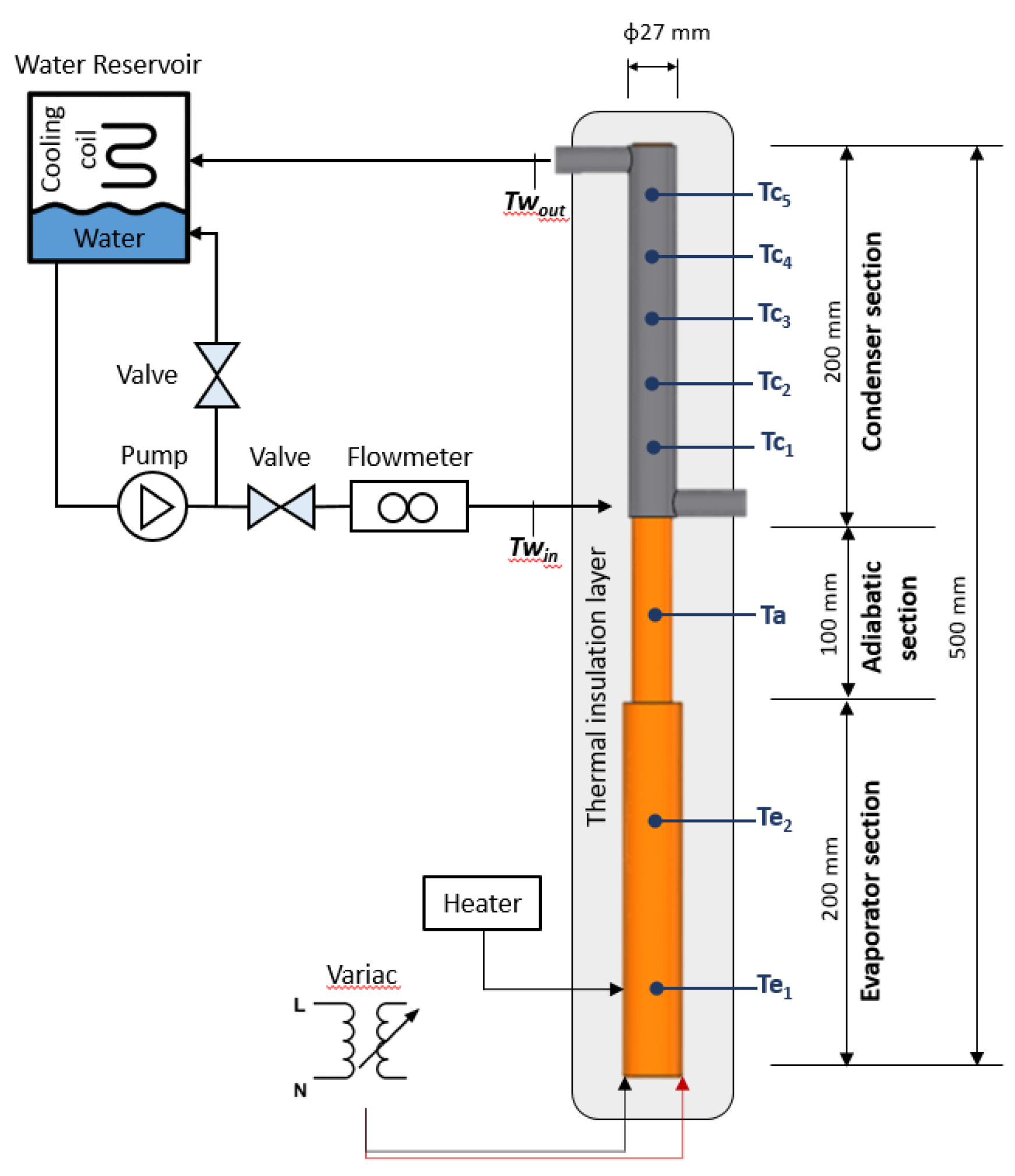
Figure 5.
CFD Block-structured mesh and boundary conditions.
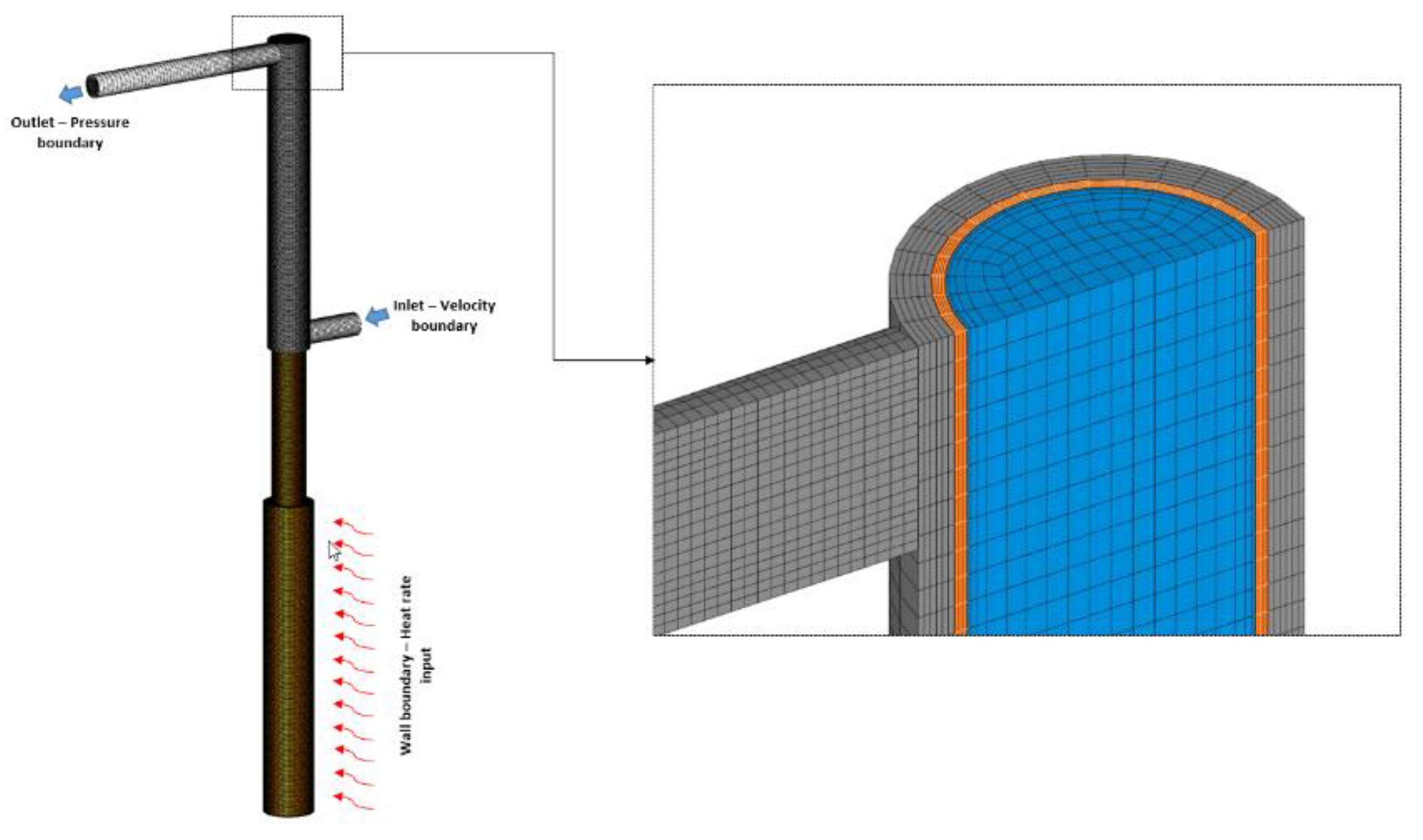
Figure 6.
Vapour pressure curve.
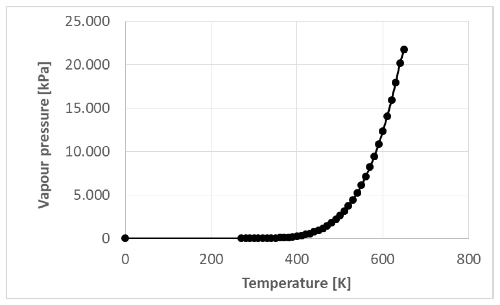
Figure 7.
(a) Steady coolant flow; (b) Outlet mass flow rate.
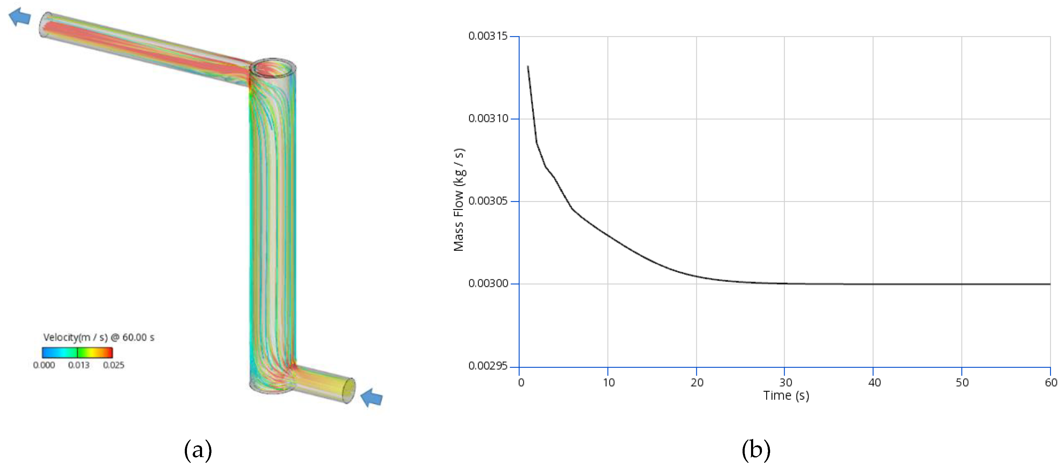
Figure 8.
(a) Water Volume Fraction distribution at 0 s, 2 s, 4 s, 8 s and 10 s for 173 W; (b) Water Volume Fraction distribution at 0 s, 2 s, 4 s, 8 s and 10 s for 376 W.
Figure 8.
(a) Water Volume Fraction distribution at 0 s, 2 s, 4 s, 8 s and 10 s for 173 W; (b) Water Volume Fraction distribution at 0 s, 2 s, 4 s, 8 s and 10 s for 376 W.
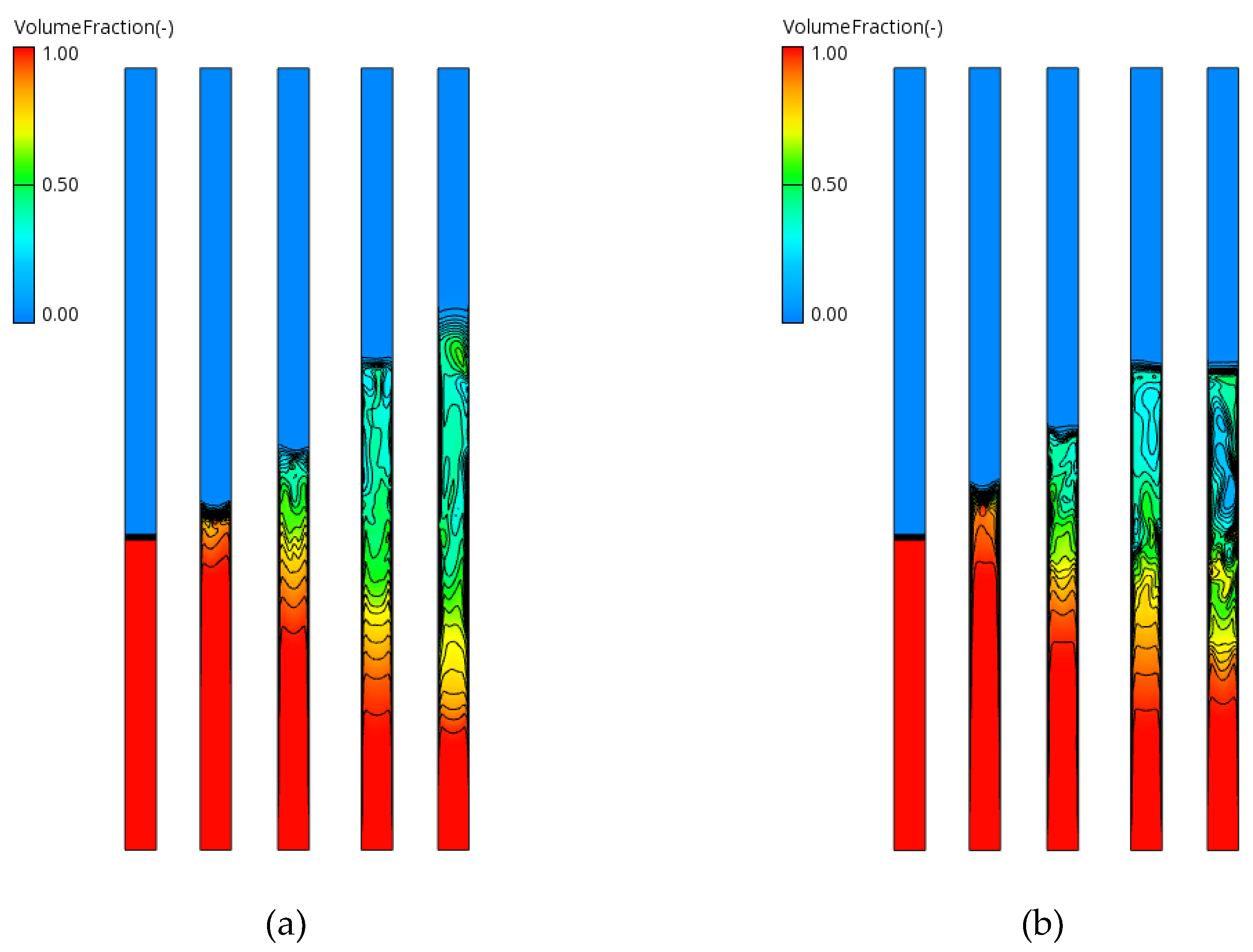
Figure 9.
Predicted condensing film formation.
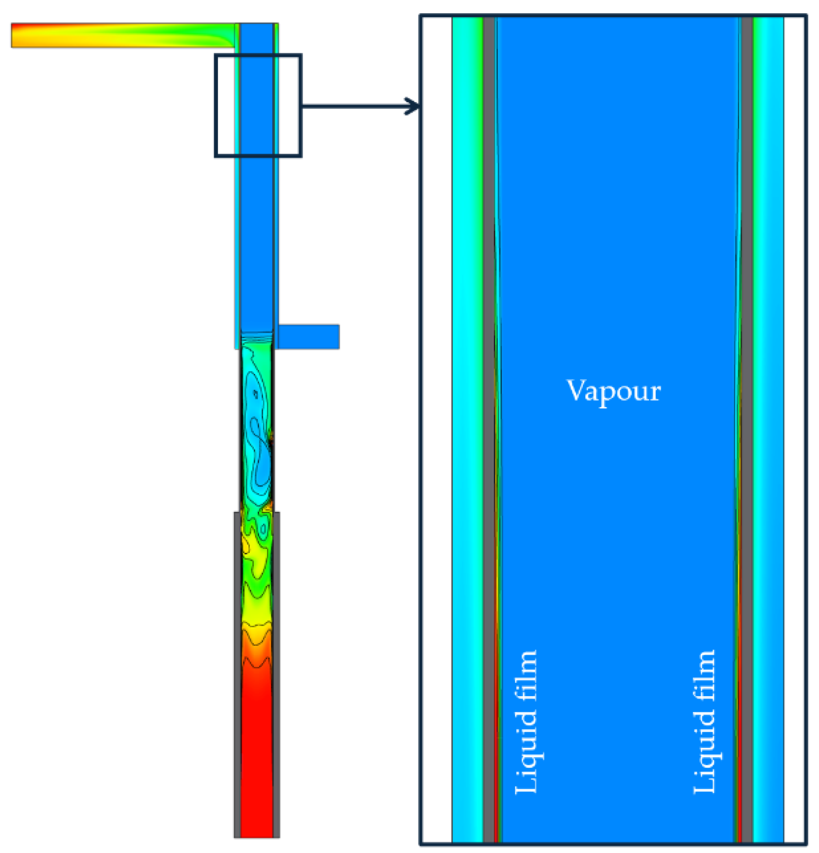
Figure 10.
(a) Heat load 173 W - Water Volume Fraction distribution at 0 s, 2 s, 4 s, 8 s and 30s; (b) Heat load 376 W - Water Volume Fraction distribution at 0 s, 2 s, 4 s, 8 s and 30 s.
Figure 10.
(a) Heat load 173 W - Water Volume Fraction distribution at 0 s, 2 s, 4 s, 8 s and 30s; (b) Heat load 376 W - Water Volume Fraction distribution at 0 s, 2 s, 4 s, 8 s and 30 s.
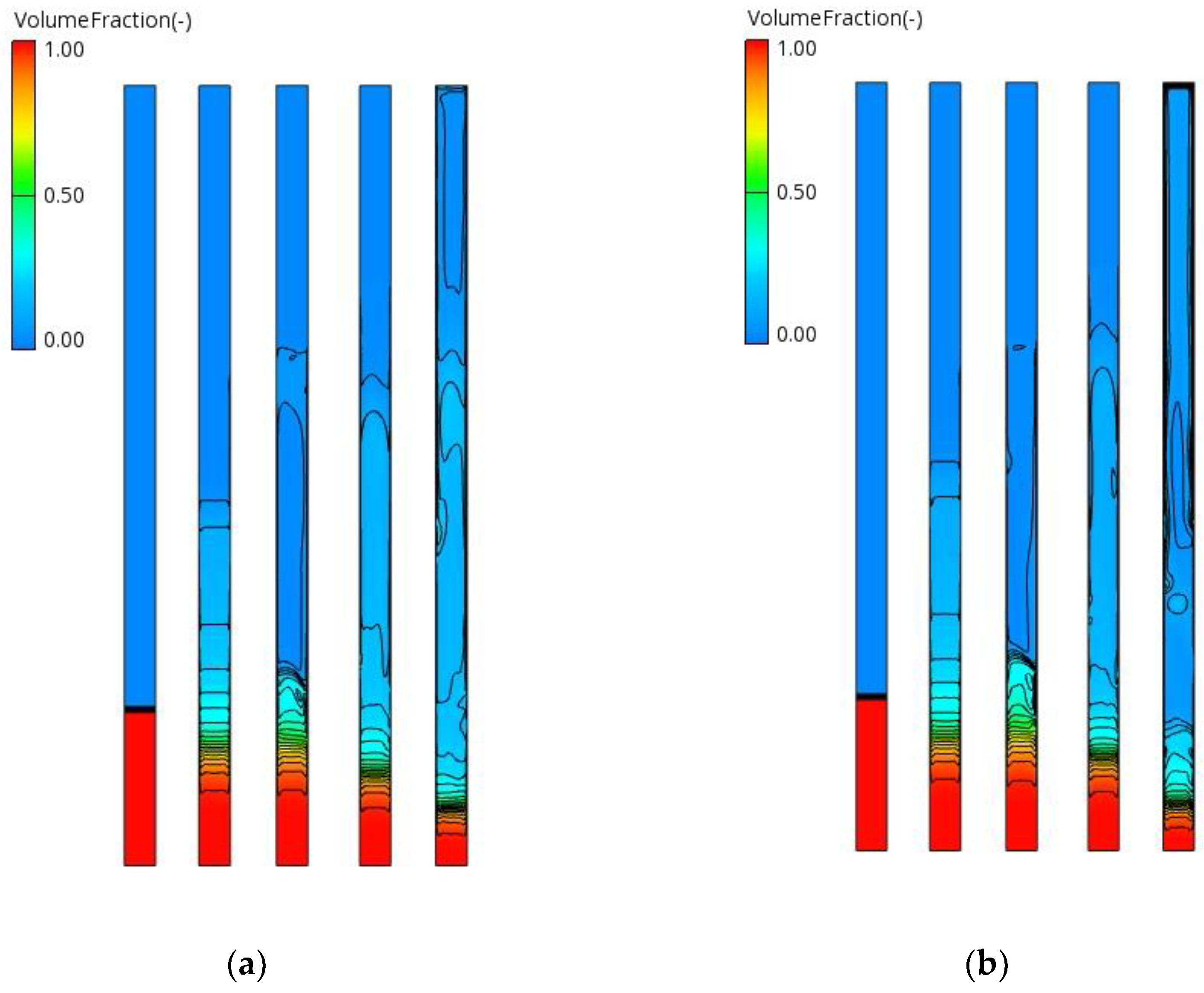
Figure 11.
Temperature distribution at various heat inputs.
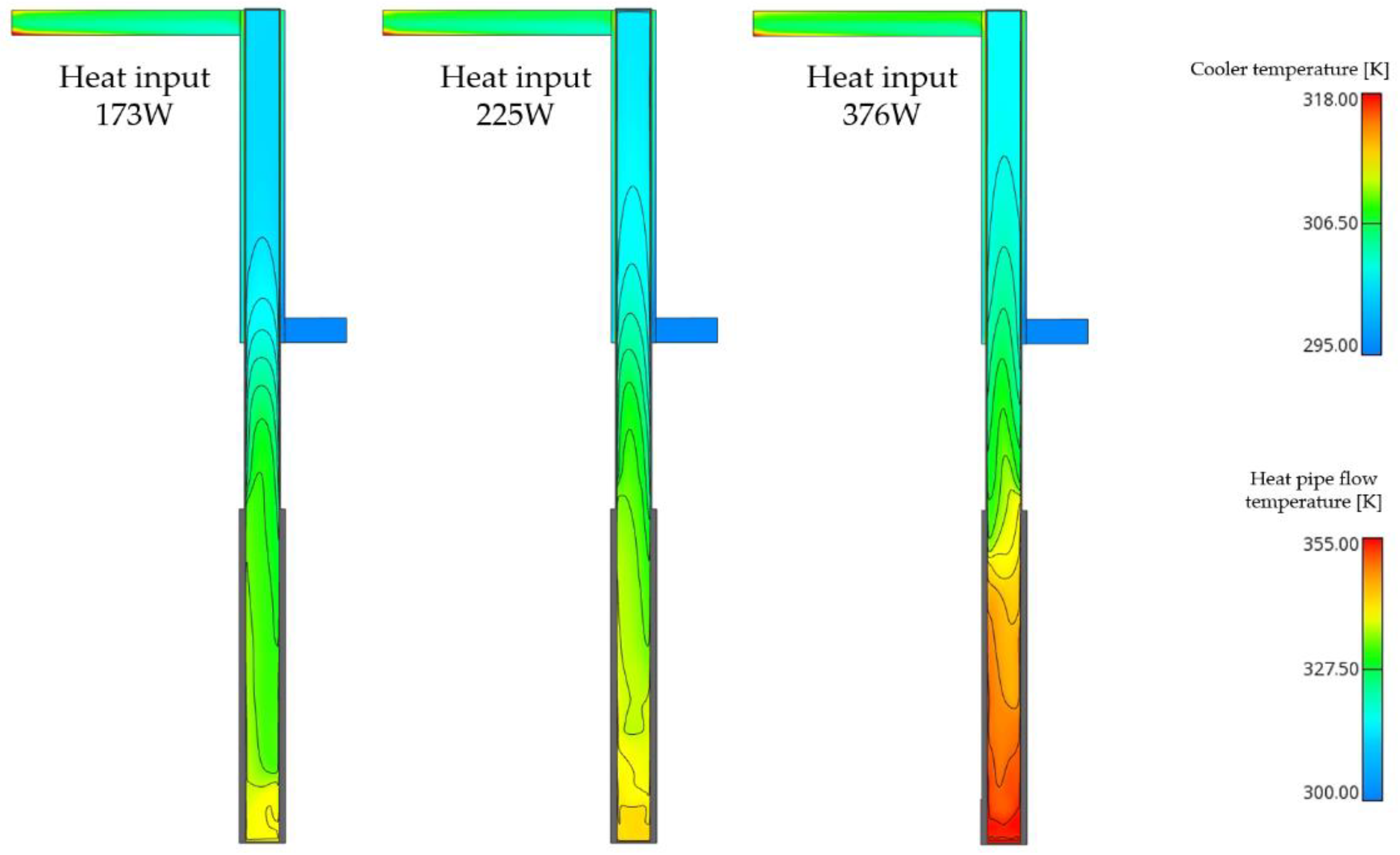
Figure 12.
Comparison of temperature distributions at various heat inputs.
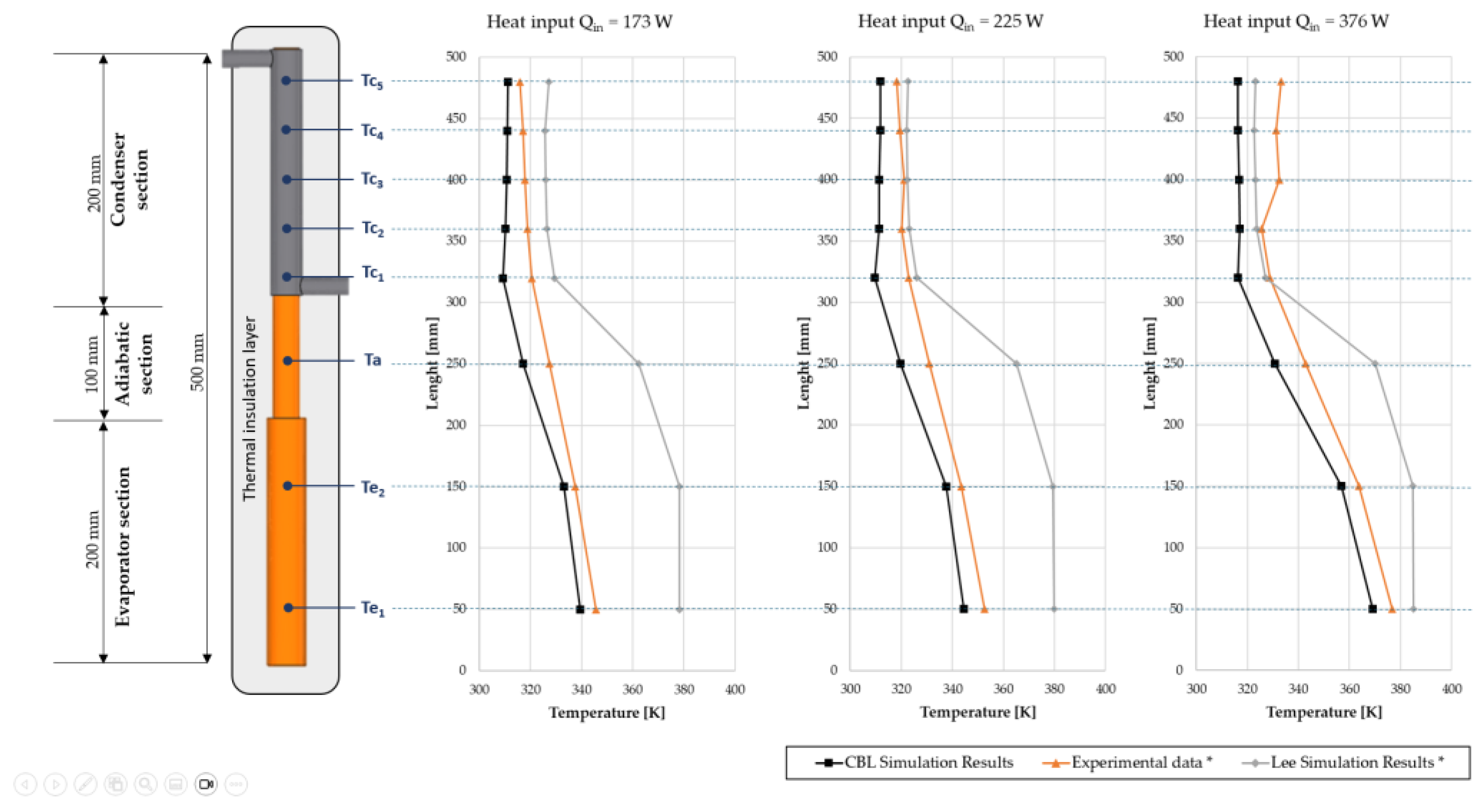

Table 1.
Transient Simulation Settings – Multiphase Fluid Domain Settings.
| System Settings | ||
| Run mode | Transient | Time step: 0.005 s |
| Number Of Iterations | Minimum: 5, Maximum 80 | |
| Module | Multiphase: | Two phases |
| Material | Liquid phase: | Gas phase: |
| Water | Vapour (ideal gas) | |
| Activate Equations | Turbulence model: | k-ε-ζ –f |
| Turbulence Wall model: | Hybrid | |
| Energy: | Static enthalpy | |
| Wall model: | Standard | |
| Additional terms | Gravity: | 9.81 m/s |
Table 2.
Multiphase interfacial exchange settings used in the simulations.
| Multiphase interfacial exchanges | CBM model |
| Momentum Interfacial exchange | “Gas Liquid System 3” Gas (c) – Liq (d): Bubble Diameter = 1 mm (Tomiyama) Drop Diameter = 0.5 mm (Schiller-Naumann) |
| Mass and Energy Interfacial exchange |
CBM model |
Table 3.
Comparison between experimental data, previous numerical results, and current CFD predictions for 173 W (50% fill ratio).
Table 3.
Comparison between experimental data, previous numerical results, and current CFD predictions for 173 W (50% fill ratio).
| Section | Monitoring position | TEXP | TCFD Lee model |
Dev Lee model |
TCFD CBL model |
Dev CBL model |
|---|---|---|---|---|---|---|
| Evaporator | Te1 | 345.75 | 378.33 | 9.42 | 339.57 | 1.79 |
| Te2 | 337.45 | 378.40 | 12.14 | 333.16 | 1.27 | |
| Adiabatic | Ta | 327.45 | 362.41 | 10.68 | 317.20 | 3.13 |
| Condenser | Tc1 | 320.55 | 329.54 | 2.80 | 309.33 | 3.50 |
| Tc2 | 318.85 | 326.54 | 2.41 | 310.26 | 2.69 | |
| Tc3 | 317.95 | 325.95 | 2.52 | 310.63 | 2.30 | |
| Tc4 | 317.09 | 325.64 | 2.71 | 310.95 | 1.94 | |
| Tc5 | 315.95 | 327.13 | 3.54 | 311.17 | 1.51 |
* Experimental data and CFD Lee model simulation results from Fadhl [8].
Table 4.
Comparison between experimental data, previous numerical results, and current CFD predictions for 225 W (50% fill ratio).
Table 4.
Comparison between experimental data, previous numerical results, and current CFD predictions for 225 W (50% fill ratio).
| Section | Monitoring position | TEXP | TCFD Lee model |
Dev Lee model |
TCFD CBL model |
Dev CBL model |
|---|---|---|---|---|---|---|
| Evaporator | Te1 | 352.68 | 379.91 | 2.72 | 344.57 | 2.30 |
| Te2 | 343.41 | 379.44 | 10.49 | 337.7 | 1.66 | |
| Adiabatic | Ta | 330.98 | 365.13 | 10.32 | 319.79 | 3.38 |
| Condenser | Tc1 | 322.93 | 326.01 | 0.95 | 309.72 | 4.09 |
| Tc2 | 320.24 | 323.15 | 0.91 | 311.38 | 2.77 | |
| Tc3 | 321.22 | 322.44 | 0.38 | 311.33 | 3.08 | |
| Tc4 | 319.51 | 322.20 | 0.84 | 311.73 | 2.43 | |
| Tc5 | 318.29 | 322.67 | 1.38 | 311.82 | 2.03 |
* Experimental data and CFD Lee model simulation results from Fadhl [8].
Table 5.
Comparison between experimental data, previous numerical results, and current CFD predictions for 376 W (50% fill ratio).
Table 5.
Comparison between experimental data, previous numerical results, and current CFD predictions for 376 W (50% fill ratio).
| Section | Monitoring position | TEXP | TCFD Lee model |
Dev Lee model |
TCFD CBL model |
Dev CBL model |
|---|---|---|---|---|---|---|
| Evaporator | Te1 | 376.75 | 385.14 | 2.23 | 369.02 | 2.05 |
| Te2 | 363.65 | 384.97 | 5.86 | 356.73 | 1.90 | |
| Adiabatic | Ta | 342.75 | 370.11 | 7.98 | 330.74 | 3.50 |
| Condenser | Tc1 | 328.95 | 327.12 | 0.56 | 316.34 | 3.83 |
| Tc2 | 325.55 | 323.66 | 0.58 | 317.00 | 2.63 | |
| Tc3 | 332.45 | 323.15 | 2.80 | 316.73 | 4.73 | |
| Tc4 | 331.35 | 322.70 | 2.61 | 316.18 | 4.58 | |
| Tc5 | 333.35 | 323.17 | 3.05 | 316.37 | 5.09 |
* Experimental data and CFD Lee model simulation results from Fadhl [8].
Disclaimer/Publisher’s Note: The statements, opinions and data contained in all publications are solely those of the individual author(s) and contributor(s) and not of MDPI and/or the editor(s). MDPI and/or the editor(s) disclaim responsibility for any injury to people or property resulting from any ideas, methods, instructions or products referred to in the content. |
© 2025 by the authors. Licensee MDPI, Basel, Switzerland. This article is an open access article distributed under the terms and conditions of the Creative Commons Attribution (CC BY) license (http://creativecommons.org/licenses/by/4.0/).
Copyright: This open access article is published under a Creative Commons CC BY 4.0 license, which permit the free download, distribution, and reuse, provided that the author and preprint are cited in any reuse.


