
Submitted:
04 November 2025
Posted:
05 November 2025
You are already at the latest version
Abstract
Leveraged exchange traded funds (LETFs) magnifying popular index daily returns by up to +/- 3.0x are often assumed to belong in the domain of sophisticated traders with short-term horizons. Despite this, eight of the top ten performing funds over the last 10 years are LETFs. This study shows why the standard method used to calculate LETF long-run expected returns relative to an underlying index produces estimates that significantly deviate from realized returns given a particular index return and standard deviation. A statistically exact equation is derived which demonstrates how current methods lead to underestimating LETF expected returns by over one hundred percentage points annually for bullish LETFs during high return/high volatility environments and equally overstate bearish LETFs performance during negative return/low volatility environments. This new method is then applied to monthly and quarterly reset LETFs showing they outperform daily LETFs in average to high volatility environments while daily LETFs tend to outperform in high return low volatility environments.
Keywords:
leveraged exchange traded funds
; long-run performance
; projecting LETF returns
; volatility correction
1. Introduction
ProShares introduced the first leveraged exchange-traded fund (LETF) in 2006 although the concept of multiplying an index’s return goes back to at least 1993 with Rydex’s 1.5x mutual fund RYNVX. However, it is within the ETF market where LETFs exploded in popularity now boasting over 170+ funds with more than $100 billion in assets multiplying a variety of underlying indexes and even individual stock returns on U.S. markets. Most of these funds multiply the underlying index’s daily return by up to +/- 3.0x although AXS Investments through Tradr introduced weekly, monthly, and quarterly return multiples in 2024. On the London Stock Exchange, there are funds that multiply daily returns up to 5.0x. On the U.S. markets, newly introduced LETFs are now limited to +/- 2.0x due to the Securities and Exchange Commission’s 2020 Derivative rule although BMO listed an exchange traded note (SPYU) with 4.0x daily leverage in December of 2023.
LETFs by their very nature magnify both the return and volatility on an underlying index by their respective leverage ratios. Over an extended holding period, LETFs experience leverage drift which is usually negative, meaning a 2.0x daily LETF will provide less than a 2.0x return beyond a day. The funds warn about these effects and highlight that these instruments are for short-term holdings. The Financial Industry Regulatory Authority (FINRA) issued a warning in June 2009 (Regulatory Notice 09-31) that “inverse and leveraged ETFs that are reset daily typically are unsuitable for retail investors who plan to hold them for longer than one trading session, particularly in volatile markets.” Some studies even suggest LETFs “converge to zero” which is generally true for inverse LETFs as they decline in value due the general upward trend of most indexes and through volatility decay, (Carver, 2009). Despite this headwind, several studies have partially dispelled the idea LETFs are only for short-term traders, (Trainor, 2011; Scott & Watson, 2013; Trainor, Chhachhi, Brown, 2020).
Although leverage decay is usually the norm, it is not a foregone conclusion if the underlying index has enough positive trend to offset leverage decay due to volatility. The projected return to a LETF relative to its underlying index is given by:
where LRT is the return to the leveraged fund, XRT is the underlying index return, β is the leverage ratio, and is the variance over the time interval T, (Cheng & Madhaven, 2009; Avellaneda & Zhang, 2010). This is the model LETF prospectuses use and is only relatively accurate for moderate return/volatility assumptions over an extended period.
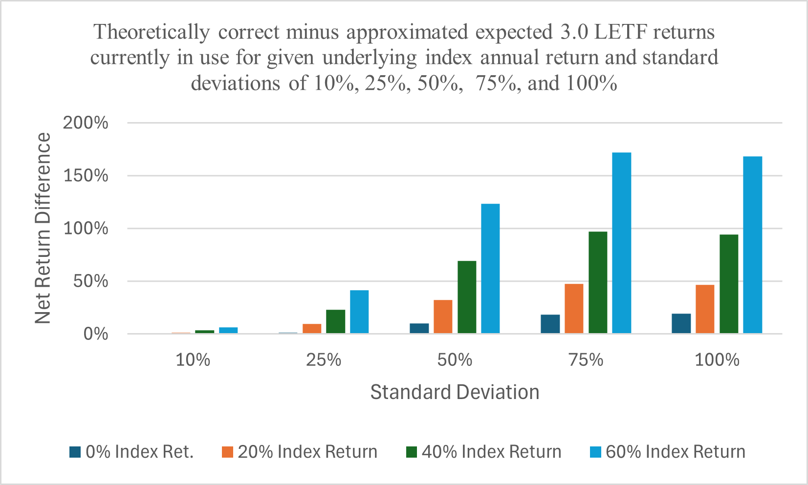
The equation’s approximation deviates from actual results because it uses an assumed variance and applies the annualized approximation method to incorrectly back out the daily variance associated with the annualized value when projecting a LETF return. Figure 1 demonstrates how large the differences are from using a statistically exact formulation relative to a derivation where approximations are used for inputs. The magnitude of this error, especially for longer holding periods, is misleading and biases the argument in favor of short-term holdings. Figure 1 shows these errors can reach up to 100% for 2.0x LETF.
Academic studies and theoretical projections aside, nothing compares to the empirical evidence many of these funds have experienced with LETFs having eight of the top ten performing funds over the last 10 years even after experiencing severe losses during one crisis or another, see Table 1. This is not unique for 2025 as LETFs often hold the top spots for 10-year returns. The extraordinary long-term gains for many of these LETFs are hard to ignore, especially for long-term buy-and-hold investors who can stomach losses of 80%+ in short periods of time. As an example, Direxion and ProShares 3.0x S&P 500 is up 1,046% and 1,043% respectively relative to SPY (291%) for an effective leverage ratio of 3.6x while Proshare’s 3.0x QQQ is up 2,516% relative to QQQ (511%) for an effective leverage ratio of 4.9x. The top performing fund is a 2.0x semi-conductor fund up 6,805%.
This study demonstrates that the current method being used to project LETF returns relative to an underlying index produces estimates that can deviate from their statistically correct values by up to +/-100% or more within a year under extreme return/volatility assumptions. The returns generated by the new method derived in this study are confirmed by Monte Carlo simulation and realized empirical results. As an additional application, comparisons are then made for daily, monthly, and quarterly reset calendar LETFs (the latter two recently introduced in 2024) showing the longer reset LETFs outperform during periods of average to high volatility and daily LETFs will outperform in periods of high trend and low volatility.
2. Statistical Approximations
2.1. Arithmetic to Geometric Mean Approximation
The current model used to estimate LETF expected returns over extended holding periods make use of the approximation methods to convert (1) an arithmetic mean into a geometric mean, and (2) conversion of a daily variance into an annualized variance.
To convert an arithmetic mean into a geometric mean, the following approximation method is used:
where is the geometric mean and is the arithmetic mean. This calculation always understates the true geometric mean although the error becomes small as the number of periods (N) approaches infinity, (McCulloch, 2003). The exact formulation is:
Figure 2 highlights the error for monthly returns based on a 1% monthly return and 5% standard deviation. For daily returns, the approximation is relatively accurate even by a month as N is large, but this is not the case for the longer reset monthly and quarterly rebalanced LETFs.
2.1. Annualizing Standard Deviation Approximation
The annualized standard deviation approximation is given by the following:
where σt is the standard deviation of period t usually specified in days or months, and N is the number of periods in a year. This is only approximately correct as the standard deviation is also a function of the return, (Tobin, 1965; Kaplan, 2012; Weber, 2017). The correct formulation is:
where μt is the expected value of the return period. The approximating formula overstates the standard deviation when the return is negative and understates when the return is positive.
Figure 3 shows how large this error can be by using the S&P 500 average daily standard deviation which is 1%. Using the approximation method, deviations from the statistically correct values range from 7% too high for a negative average daily return of -0.25% (-47% annualized…but only approximately) to 14% too low for a 0.25% daily return (88% annualized, approximately).
This is especially relevant to LETFs as they magnify both the daily return and standard deviation by their leverage ratio. Relative to any underlying index, LETF’s annual standard deviation over time is not just leverage times the annual standard deviation of the index, but the leverage times the underlying index’s daily mean and standard deviation (week, month, or quarter for the new calendar LETFs) within Equation (5). The correct formulation where L is the leverage ratio is shown in Equation (6):
Both issues above are exaggerated for LETFs. Thus, when one poses the question of how would a 3.0x LETF perform over a year when the underlying index experiences a 50% annual return with a 40% standard deviation, the approximation formula should not be used to (1) back out the index daily return and standard deviation, then (2) calculate the LETF’s daily return and standard deviation, to then (3) calculate a geometric return, and then (4) annualize once again using an approximation formula. The larger the mean and standard deviation assumed, the greater the deviation from the statistically exact value.
In practice, with the underlying index returns deviating from normality, serial dependence, tracking error, expense ratios, financing costs, etc., there will be deviations from any theoretical exact value attained. However, a correct derivation is necessary for investors making long-term investment decisions involving the use of LETFs. This theoretically correct formulation reduces the evidence to some degree against longer-term holdings of LETFs.
3. Calculating LETF Expected Returns Relative to Underlying Index
3.1. The Approximation Method for LETF Expected Returns
The current method used to approximate expected returns for LETFs for an annual holding period inputs an assumed underlying annualized index return and standard deviation. For daily rebalanced LETFs, the underlying index geometric daily return is calculated based on Equation (7):
where RA is the annual return and N is assumed to be 252 for trading days in a year. Using the approximation in Equation (7), the arithmetic mean return (μt) is found by adding where the daily standard deviation is approximated using Equation (4) by solving for . This is necessary as the daily arithmetic mean must exceed the daily geometric return to attain the original annual return. The annualized LETF return RL can now be calculated as shown below:
This replicates typical tables found in the prospectuses of daily LETF providers with minor differences of less than 0.1% even at the higher annualized index return and volatility assumptions. The various prospectuses themselves apply Equation (1) which was derived under a continuous time setting that also uses the approximations in Equations (2) and (4) for its derivation. The calculations from Equations (1) or (8) give the same basic results, (see Direxion (2025, GraniteShares (2025), or Proshares (2025) prospectuses, but all LETF fund providers use this method to create their long-run return tables).
However, when using the above method, the realized annual return and standard deviation of an underlying index is significantly different from the assumed annual return and standard deviation for the more extreme return/volatility assumptions. Table 2 shows the assumed underlying index annual return/volatility pairs and the numerical Monte Carlo (100,000) simulated volatility that is realized.
At low levels of volatility, the numerical results align functionally well with the approximations except for the biased volatility. However, with a standard deviation of 50%, the results begin to significantly deteriorate with higher returns such as the assumed 40%/50% return/volatility pair which numerically results in a 59% mean return and 84% volatility. It should be noted that the median returns are exact as they are not affected by the erroneous standard deviations.
However, this is not helpful as the standard deviation is the primary factor that erodes LETF returns over time relative to an underlying index. With an assumed annual return of 60% and volatility of 100%, the actual mean/volatility pair using the approximation method is 163% and 339% respectively. Thus, this method’s calculations are going to significantly deviate from using a statistically exact formulation for estimating LETF returns where the deviation will increase with greater leverage, higher absolute return/volatility assumptions, and time.
3.2. Statistically Exact Formulation for LETF Expected Return
To calculate statistically correct values for LETFs, the exact daily arithmetic mean and daily standard deviation for the underlying index can be calculated by solving for in Equation (5). This gives the following:
This value can then be substituted into Equation (3) resulting in Equation (10):
There is no closed form solution for the daily arithmetic index return but it can be solved for iteratively until a given assumed is found. This is then substituted back into Equation (9) to calculate . These are theoretically exact values for the daily return and standard deviation that will give the exact annual standard deviation that is originally assumed. For large t, from Equation (9) could be inserted into Equation (2) to simplify but would still need to be solved for iteratively.
It should be noted that the initially assumed annual return will not equal the annualized geometric return since compounded returns are not normally but lognormally distributed. By (1) starting out with an assumed annual mean and standard deviation, then (2) finding the daily arithmetic mean and standard deviation that results in a daily geometric mean (given a daily standard deviation), that can then (3) be annualized to reattain the originally given annual return and standard deviation is not the same as the realized annual mean given volatility around the geometric mean. The daily returns will be normally distributed using the above, but after compounding to reacquire an annualized return results in a lognormal distribution with a realized mean greater than the original.
However, the median will be exactly the original annual return value and thus, armed with the correct standard deviation, an exact estimate of the central tendency for LETFs returns can be made. The LETF daily return/volatility values are simply the daily leverage times the mean and standard deviation found from Equations (9) and (10) which can be inserted in Equations (3) and (5) where Lμt and Lσt are substituted in place of μt and σt to calculate the annual LETF return and standard deviation. Theoretical results are verified using 100,000 Monte Carlo simulations per return/volatility pair.
Table 3 Panel A shows a typical table found in the prospectus of multiple fund providers for a 2.0x daily LETF over a year for a given underlying index return and volatility. Panel A shows the approximation method (Equation 1) while Panel B shows the results from the exact method. The shaded cells are those returns that are less than 2.0x times the index which occurs in high volatility environments due to compounding drag associated with these funds.
The approximation works relatively well for extreme negative returns regardless of the volatility, but deviations from the statistically exact method become quite large the higher the assumed annual return and standard deviation. This is especially obvious when comparing the last rows of Panels A and B with a 50% or greater volatility where the deviation reaches over 100% for the 60%/100% return/volatility assumption. All values in Table 3 are confirmed using Monte Carlo methods with differences of less than 1.0% even at extremes. Although the calculated daily returns using the approximation or theoretically exact method do not substantially differ, it is the use of the approximation formula to calculate the standard deviation which is the culprit for most of the dispersion.
To demonstrate how leverage affects the results, Table 4 shows the comparison values for a 3.0x with shaded cells showing when the return is less than 3.0x the index. The difference between the two methods becomes large even when assuming a moderate 25% volatility at the higher return levels. Because the approximation method overestimates the daily standard deviation to such an extent with high return assumptions, the expectation using the approximation method at the 60%/75% return/volatility results in a -24.2% return instead of the statistically correct value of 147.6%. Increasing the time horizon would further distort these values as evidenced by the historical returns to these funds.
To give an empirical example, ProShares USD was the top performing fund over the last 10 years with its latest one-year return ending 10/31/2025 earning 90.4%% while the DJ U.S. Semi-conductor index increased 58.4%, see Table 5. Assuming zero costs, a perfect daily 2.0x should have earned 108.2%. The differences are trading costs, financing costs, expense ratio, and tracking error. The index’s daily return and standard deviation was 0.22% and 2.72% respectively over this year and based on statistically exact annualization an annual standard deviation of 78.7% is calculated reaffirmed using Monte Carlo simulation.
The approximation method using 58.4%/78.7% return/volatility inputs predicts this annual return to be 35% while the statistically correct method predicts 109.8%, almost exactly the result from a perfect 2.0x daily return over this period. For a -2.0x, the approximation method calculates a -94% loss for a -2.0x while the exact method calculates -77.5% which is exactly what occurred both for a perfect daily -2.0x (-77.5%) and what ProShares (-74%) basically provided.
The year ending 10/31/2024 tells the same story while the last column of Table 5 uses year ending 12/29/22 when the index was down 39.43%. Results are as expected where the approximation method significantly deviates from both the statistically exact method and empirical results, the latter two aligning almost perfectly. In this case, the approximation significantly overestimates (projected 100.1%) to what a perfect -2.0x attains (46.8%).
One final note should be made, Equation (1) works quite well ex-post, meaning that if one inputs the realized daily average return and daily standard deviation, the predicted LETF returns are quite accurate for extended holding periods. The error occurs when one starts with an assumed annual return and standard deviation and attempts to predict what would occur with those inputs. The approximations used to calculate the daily return and daily standard deviation from these inputs and then used by Equation (1) leads to significant errors when these inputs are relatively large.
3.3. Statistically Exact Formulation for Inverse LETF Expected Return
Expected returns for inverse funds are significantly overestimated for yearly periods for declining markets (by over 200% in some cases), but with market trends generally up, long-term holdings of these funds are not advised even for the most bearish investor. One of the issues is that declining markets are generally accompanied by high volatility which mitigates expected gains from LETFs. Since leverage is required even for -1.0x funds, calculations using the approximation method deviate from statistically exact values even at this level. Table 6 shows the approximation and statistically exact method for expected 2.0x LETF returns with greater deviations occurring for high negative returns regardless of volatility.
3.4. Statistically Exact Method for Daily, Monthly, & Quarterly LETF Expected Returns
Daily vs monthly vs quarterly reset LETFs can now be directly compared for any time horizon. For a year, simply set t = 252, 12, or 4 respectively in equations (9) and (10). Table 7, Panels A, B, and C display the results using the statistically exact method for all three 2.0x LETFs. For low levels of volatility, the daily LETFs marginally outperform the monthly but as volatility increases, the monthly LETFs outperform unless the trend is high enough to offset the higher volatility. After 50% volatility, the trend would need to be even higher than 60% to outperform the monthly LETFs.
The same types of results occur for quarterly reset LETFs. For low levels of volatility and high trend, the daily and monthly LETFs outperform but quarterly LETFs outperform at high volatility levels regardless of the trend as can be seen in the last two columns. As there are currently no monthly or quarterly reset inverse LETFs, those results are not reported.
4. Discussion
LETFs have slowly moved into the mainstream with now more than 170+ funds containing $100 billion plus in assets. Originally recommended only to sophisticated investors with short-term holding periods, historical results suggest this recommendation may be too conservative as these funds are often at the top of 10-year performance winners. However, these funds do have significant risk as large losses can occur very quickly, especially at higher leverage ratios. For those wanting to accept this risk, there has been generous compensation over the last ten years for many of the most popular indexes.
The current method used by LETF providers in their prospectuses to show expected returns for theoretical annual holding periods of LETFs relative to an underlying index underestimates the long-run returns of these funds biasing evidence towards concluding LETFs should be mainly limited to short-term holdings. Deviations from statistically exact values are significant (greater than 100% in cases) for high return/volatile environments with semi-conductors being a prime example. This study derives statistically correct expected returns for given annual return/volatility assumption showing that bullish LETF returns are underestimated in high return/volatility environments while inverse LETF returns are overestimated in extreme negative/low volatility environments when using approximation methods.
Using statistically exact formulations, this study goes on to show how the recently introduced monthly and quarterly rebalance LETFs significantly outperform daily LETFs during higher volatility environments while daily LETFs outperform in high trend/low volatility environments. The use of the model derived in this study improves long-term LETF investor’s information set when determining the suitability of the various LETF funds available.
Funding
This research received no external funding.
Institutional Review Board Statement
Not applicable.
Informed Consent Statement
Not applicable.
Data Availability Statement
Return data used is available from finance.yahoo.com, ETFvest.com, Proshares.com for NAV data, and SPglobal.com.
Conflicts of Interest
The author declares no conflicts of interest.
Abbreviations
The following abbreviations are used in this manuscript:
| LETF | Leverage Exchange Traded Fund |
| FINRA | Financial Industry Regulatory Authority |
References
- Avellaneda, M.; Zhang, S. Path-dependence of Leverage ETF returns. Society for Industrial and Applied Mathematics 2010, 1, 586–603. [Google Scholar]
- Carver, A. Do leveraged and inverse ETFs converge to zero? Institutional Investor Journals, ETFs and Indexing 2009, 1, 144–149. [Google Scholar]
- Cheng, M.; Madhavan, A.A. The dynamics of leveraged and inverse exchange-traded funds. Journal of Investment Management 2009, 7, 43–62. [Google Scholar]
- Direxion Prospectus. Available online: https://connect.rightprospectus.com/Direxion/TVT/25461H101/P (accessed on 12 June 2025).
- Graniteshares Prospectus. Available online: https://graniteshares.com/media/w2llat0w/graniteshares-etf-trust-s-l-single-stock-etfs-prospectus.pdf?hsCtaAttrib=193774651499 (accessed on 24 October 2025).
- Kaplan, D. What’s wrong with multiplying by the square root of twelve. Journal of Performance Measurement 2012, 17, 16–24. [Google Scholar]
- McCulloch, B. Geometric return and portfolio analysis. New Zealand Treasury, 2003.
- Proshares Prospectus. Available online: https://www.proshares.com/regulatory-document-viewer-page?ticker=SSO&document-label=statutory-prospectus (accessed on 26 September 2025).
- Scott, J.; Watson, J. The floor-leverage rule for retirement. Financial Analysts Journal 2013, 69, 45–60. [Google Scholar] [CrossRef]
- Tobin, J. The theory of portfolio selection. In The Theory of Interest Rates; Hahn, F., Brechling, F., Eds.; Macmillan Publishing: London, 1965. [Google Scholar]
- Trainor, W. Solving the leveraged ETF compounding problem. Journal of Index Investing 2011, 1, 66–74. [Google Scholar] [CrossRef]
- Trainor, W.; Chhachhi, I.; Brown, C. A portfolio of leveraged ETFs. Financial Services Review 2020, 28, 35–48. [Google Scholar] [CrossRef]
- Weber, A. Annual risk measures and related statistics. Ortec Finance Research Center, Applied paper No. 2017-01, 1-19. (Davison, 1623/2019) Davison, T. E. (2019). Title of the book chapter. In A. A. Editor (Ed.), Title of the book: Subtitle (pp. Firstpage–Lastpage). Publisher Name. (Original work published 1623) (Optional) 2017.
Figure 1.
2.0x LETF One Year Theoretically Correct Minus Approximate Return for Given Index Return and Standard Deviation.
Figure 1.
2.0x LETF One Year Theoretically Correct Minus Approximate Return for Given Index Return and Standard Deviation.
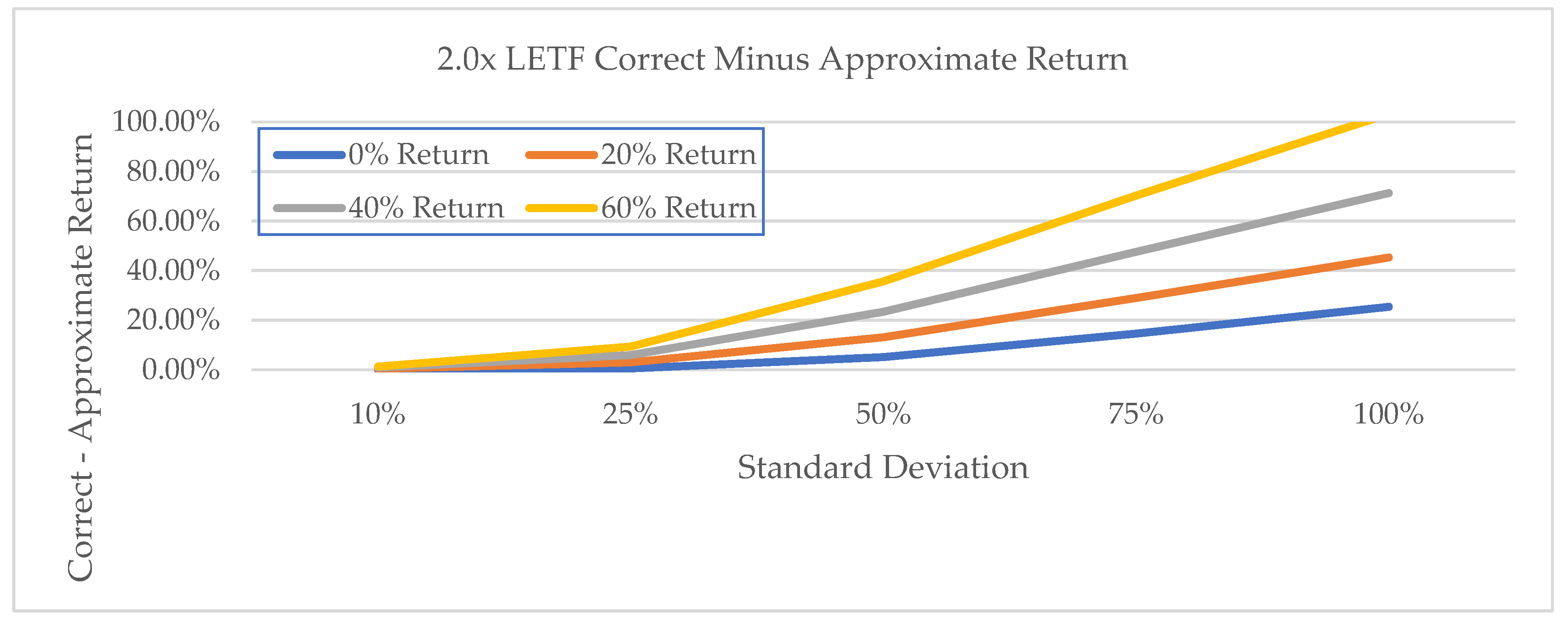
Figure 2.
Theoretical and Approximate Geometric Returns for a 1% Monthly Mean Return with 5% standard deviation.
Figure 2.
Theoretical and Approximate Geometric Returns for a 1% Monthly Mean Return with 5% standard deviation.
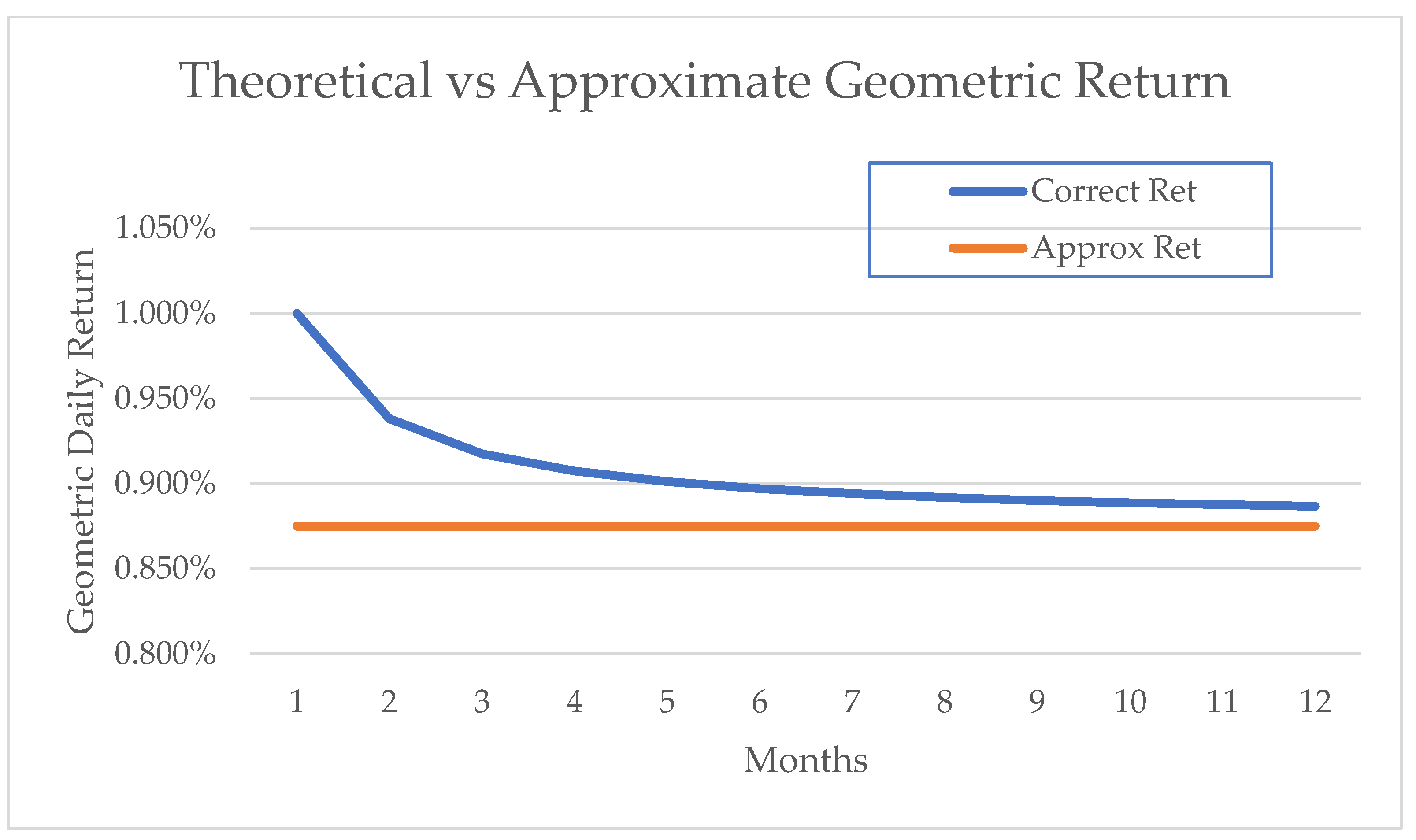
Figure 3.
Theoretical and Approximate Annualized Standard Deviation Relative to Daily Mean Return with 1% standard deviation.
Figure 3.
Theoretical and Approximate Annualized Standard Deviation Relative to Daily Mean Return with 1% standard deviation.
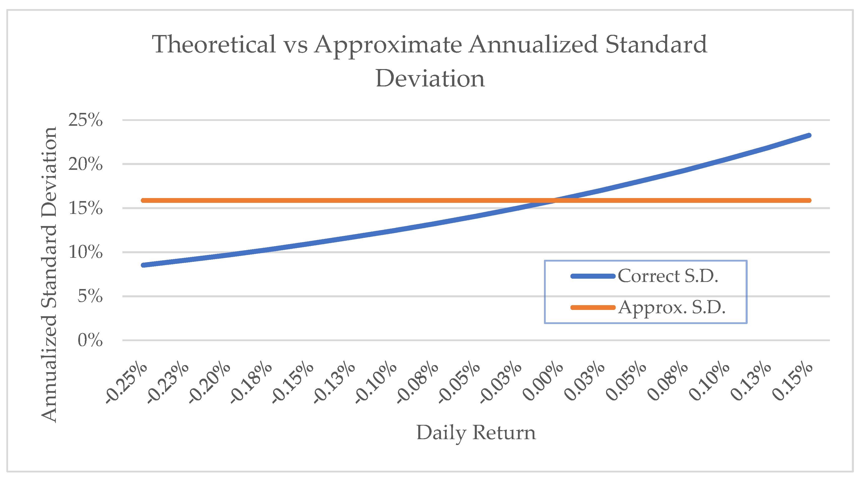

Table 1.
Top ETF Performers 10-years ending 10/17/2025.
| Ticker | Fund | Leverage | 10-year return, 10/17/2025 |
| USD | ProShares Semiconductors | 2x | 6,805% |
| TECL | Direxion Technology 3x ETF | 3x | 3,829% |
| SOXL | Direxion Semiconductor 3x ETF | 3x | 2,734% |
| TQQQ | ProShares QQQ 3x ETF | 3x | 2,516% |
| ROM | ProShares Technology 2x ETF | 2x | 1,968% |
| QLD | ProShares QQQ 2x ETF | 2x | 1,474% |
| SMH | VanEck Semiconductor ETF | 1x | 1,367% |
| SPXL | Direxion S&P 500 3x ETF | 3x | 1,046% |
| UPRO | ProShares S&P 500 3x ETF | 3x | 1,043% |
| SOXX | iShares Semiconductor ETF | 1x | 1,025% |
Source: ETFvest.com.
Table 2.
Selected annual return/volatility pairs and realized results using Monte Carlo simulation based on approximation methods for calculating the daily return and volatility.
Table 2.
Selected annual return/volatility pairs and realized results using Monte Carlo simulation based on approximation methods for calculating the daily return and volatility.
| Assumed Volatility | |||||
| Assumed Index Return |
10% | 25% | 50% | 75% | 100% |
| -60% | 60%, 4% | -59%, 11% | -55%, 24% | -47%, 46% | -34%, 86% |
| -40% | -40%, 6% | -38%, 16% | -32%, 36% | -20%, 69% | -1%, 129% |
| -20% | -20%, 8% | -17%, 21% | -9%, 48% | 6%, 93% | 32%, 175% |
| 0% | 0%, 10% | 3%, 26% | 13%, 60% | 32%, 114% | 64%, 212% |
| 20% | 21%, 12% | 24%, 31% | 36%, 72% | 60%, 139% | 97%, 254% |
| 40% | 41%, 14% | 44%, 36% | 59%, 84% | 86%, 160% | 128%, 292% |
| 60% | 61%, 16% | 65%, 42% | 81%, 96% | 112%, 181% | 163%, 339% |
Table 3.
Expected returns over a year for a 2.0x LETF with a given underlying index annual return and standard deviation.
Table 3.
Expected returns over a year for a 2.0x LETF with a given underlying index annual return and standard deviation.
| Panel A: Approximation Method | ||||||||||
| Index Return / Volatility | 10% | 25% | 50% | 75% | 100% | |||||
| -60% | -84.2% | -85.0% | -87.5% | -90.9% | -94.1% | |||||
| -40% | -64.4% | -66.2% | -72.0% | -79.5% | -86.8% | |||||
| -20% | -36.6% | -39.9% | -50.2% | -63.5% | -76.5% | |||||
| 0% | -1.0% | -6.1% | -22.1% | -43.0% | -63.2% | |||||
| 20% | 42.6% | 35.3% | 12.1% | -18.0% | -47.0% | |||||
| 40% | 94.0% | 84.1% | 52.6% | 11.7% | -27.9% | |||||
| 60% | 153.5% | 140.5% | 99.4% | 45.9% | -5.8% | |||||
| Panel B: Exact Method | ||||||||||
| Index Return / Volatility | 10% | 25% | 50% | 75% | 100% | |||||
| -60% | -84.9% | -87.7% | -91.3% | -93.4% | -94.7% | |||||
| -40% | -65.0% | -68.8% | -75.5% | -80.4% | -83.8% | |||||
| -20% | -37.0% | -41.3% | -50.7% | -58.9% | -65.1% | |||||
| 0% | -1.0% | -5.5% | -17.0% | -28.4% | -37.8% | |||||
| 20% | 43.0% | 38.3% | 25.3% | 11.0% | -1.7% | |||||
| 40% | 94.9% | 90.1% | 76.0% | 59.3% | 43.4% | |||||
| 60% | 154.8% | 149.9% | 135.0% | 116.2% | 97.4% | |||||
Table 4.
Expected returns over a year for a 3.0x LETF with a given underlying index annual return and standard deviation.
Table 4.
Expected returns over a year for a 3.0x LETF with a given underlying index annual return and standard deviation.
| Panel A: Approximation Method | ||||||||||
| Index Return / Volatility | 10% | 25% | 50% | 75% | 100% | |||||
| -60% | -93.8% | -94.7% | -97.0% | -98.8% | -99.7% | |||||
| -40% | -79.0% | -82.1% | -89.8% | -96.0% | -98.9% | |||||
| -20% | -50.3% | -57.6% | -75.8% | -90.5% | -97.5% | |||||
| 0% | -3.0% | -17.1% | -52.8% | -81.5% | -95.0% | |||||
| 20% | 67.7% | 43.3% | -18.4% | -68.0% | -91.4% | |||||
| 40% | 166.3% | 127.5% | 29.6% | -49.2% | -86.3% | |||||
| 60% | 297.5% | 239.6% | 93.5% | -24.2% | -79.6% | |||||
| Panel B: Exact Method | ||||||||||
| Index Return / Volatility | 10% | 25% | 50% | 75% | 100% | |||||
| -60% | -94.7% | -97.1% | -99.0% | -99.5% | -99.8% | |||||
| -40% | -80.1% | -85.9% | -93.2% | -96.5% | -98.0% | |||||
| -20% | -51.1% | -60.4% | -76.6% | -86.3% | -91.6% | |||||
| 0% | -2.9% | -15.7% | -42.8% | -63.1% | -75.7% | |||||
| 20% | 69.2% | 53.0% | 13.9% | -20.5% | -44.6% | |||||
| 40% | 170.0% | 150.4% | 98.9% | 47.8% | 8.2% | |||||
| 60% | 303.9% | 281.0% | 217.1% | 147.6% | 88.9% | |||||
Table 5.
Comparison of approximate and exact expected returns for semi-conductor +/-2.0x LETFs.
| Year ending: | 10/31/2025 | 10/31/2024 | 12/29/2022 |
| DJ Semi-Conductor Index Return | 58.4% | 115.2% | -39.4% |
| Perfect Daily 2.0x | 108.2% | 293.7% | -70.1% |
| ProShares USD 2.0x | 90.4% | 267.1% | -71.5% |
| Approximation 2.0x Method | 35.2% | 81.0% | -66.9% |
| Exact 2.0x Method | 109.8% | 295.0% | -70.2% |
| Perfect Daily -2.0x | -77.5% | -86.8% | 46.8% |
| ProShares SSG -2.0x | -71.4% | -85.9% | 50.8% |
| Approximation -2.0x Method | -93.9% | -98.7% | 100.1% |
| Exact -2.0x Method | -77.5% | -86.8% | 47.5% |
Table 6.
Expected returns over a year for a -2.0x LETF with a given underlying index annual return and standard deviation.
Table 6.
Expected returns over a year for a -2.0x LETF with a given underlying index annual return and standard deviation.
| Panel A: Approximation Method | ||||||||||
| Index Return / Volatility | 10% | 25% | 50% | 75% | 100% | |||||
| -60% | 506.5% | 418.1% | 195.2% | 15.6% | -68.9% | |||||
| -40% | 169.6% | 130.3% | 31.2% | -48.6% | -86.2% | |||||
| -20% | 51.6% | 29.5% | -26.2% | -71.1% | -92.2% | |||||
| 0% | -3.0% | -17.1% | -52.8% | -81.5% | -95.0% | |||||
| 20% | -32.6% | -42.4% | -67.2% | -87.2% | -96.5% | |||||
| 40% | -50.5% | -57.7% | -75.9% | -90.6% | -97.5% | |||||
| 60% | -62.1% | -67.6% | -81.5% | -92.8% | -98.1% | |||||
| Panel B: Exact Method | ||||||||||
| Index Return / Volatility | 10% | 25% | 50% | 75% | 100% | |||||
| -60% | 422.9% | 185.8% | 1.6% | -55.6% | -77.1% | |||||
| -40% | 155.9% | 82.7% | -12.0% | -55.2% | -74.8% | |||||
| -20% | 49.2% | 20.9% | -28.6% | -58.8% | -75.0% | |||||
| 0% | -2.9% | -15.8% | -43.1% | -63.6% | -76.4% | |||||
| 20% | -32.0% | -38.6% | -54.5% | -68.5% | -78.3% | |||||
| 40% | -49.8% | -53.5% | -63.2% | -72.9% | -80.4% | |||||
| 60% | -61.5% | -63.7% | -69.9% | -76.7% | -82.4% | |||||
Table 7.
Exact expected returns for daily, monthly, and quarterly reset LETF over a year for 2.0x LETFs with a given underlying index annual return and standard deviation.
Table 7.
Exact expected returns for daily, monthly, and quarterly reset LETF over a year for 2.0x LETFs with a given underlying index annual return and standard deviation.
| Panel A: Daily 2.0x Leverage | ||||||||||
| Index Return / Volatility | 10% | 25% | 50% | 75% | 100% | |||||
| -60% | -84.9% | -87.7% | -91.3% | -93.4% | -94.7% | |||||
| -40% | -65.0% | -68.8% | -75.5% | -80.4% | -83.8% | |||||
| -20% | -37.0% | -41.3% | -50.7% | -58.9% | -65.1% | |||||
| 0% | -1.0% | -5.5% | -17.0% | -28.4% | -37.8% | |||||
| 20% | 43.0% | 38.3% | 25.3% | 11.0% | -1.7% | |||||
| 40% | 94.9% | 90.1% | 76.0% | 59.3% | 43.4% | |||||
| 60% | 154.8% | 149.9% | 135.0% | 116.2% | 97.4% | |||||
| Panel B: Monthly 2.0x Leverage | ||||||||||
| Index Return / Volatility | 10% | 25% | 50% | 75% | 100% | |||||
| -60% | -86.1% | -88.8% | -91.6% | -92.9%* | -93.7%* | |||||
| -40% | -65.8% | -69.4% | -75.3%* | -79.0%* | -81.3%* | |||||
| -20% | -37.2% | -41.2%* | -49.5%* | -56.1%* | -60.6%* | |||||
| 0% | -0.9%* | -5.0%* | -15.0%* | -24.2%* | -31.4%* | |||||
| 20% | 42.7% | 38.6%* | 27.6%* | 16.2%* | 6.5%* | |||||
| 40% | 93.4% | 89.3% | 77.7%* | 64.5%* | 52.5%* | |||||
| 60% | 150.7% | 146.7% | 134.9%* | 120.4%* | 106.3%* | |||||
| Panel C: Quarterly 2.0x Leverage | ||||||||||
| Index Return / Volatility | 10% | 25% | 50% | 75% | 100% | |||||
| -60% | -88.9% | -91.1% | -92.3% | -92.4%* | -92.1%* | |||||
| -40% | -67.6% | -70.9% | -74.9%* | -76.5%* | -77.0%* | |||||
| -20% | -37.7% | -41.1%* | -47.3%* | -51.1%* | -53.1%* | |||||
| 0% | -0.7%* | -4.0%* | -11.3%* | -17.1%* | -20.8%* | |||||
| 20% | 42.2% | 39.2%* | 31.6%* | 24.3%* | 19.0%* | |||||
| 40% | 90.4% | 87.6% | 80.0%* | 71.9%* | 65.1%* | |||||
| 60% | 143.1% | 140.6% | 133.2%* | 124.6%* | 116.8%* | |||||
*Greater than daily LETF return.
Disclaimer/Publisher’s Note: The statements, opinions and data contained in all publications are solely those of the individual author(s) and contributor(s) and not of MDPI and/or the editor(s). MDPI and/or the editor(s) disclaim responsibility for any injury to people or property resulting from any ideas, methods, instructions or products referred to in the content. |
© 2025 by the authors. Licensee MDPI, Basel, Switzerland. This article is an open access article distributed under the terms and conditions of the Creative Commons Attribution (CC BY) license (http://creativecommons.org/licenses/by/4.0/).
Copyright: This open access article is published under a Creative Commons CC BY 4.0 license, which permit the free download, distribution, and reuse, provided that the author and preprint are cited in any reuse.


