
Submitted:
04 September 2024
Posted:
04 September 2024
You are already at the latest version
Abstract
Recent algorithmic-based research in the stock market has predominantly focused on ultra-high-frequency trading and index estimation. We developed an improved algorithm to address the need for a low-frequency, real-world trading model to build on the existing high hit-ratio and low maximum drawdown. We utilized established price indicators, Stochastic and Williams %R, and introduced a volume factor to increase the model's safety to enhance the model's performance. This improved algorithm demonstrated superior returns while maintaining high hit-ratio and low maximum drawdown. Specifically, we leveraged the existing algorithm to trade using 2X and 3X signals, incorporating volume data, the 52-week average, standard deviation, and other factors. The data set comprised SPY ETF price and volume from 2010 to 2023, covering over 13 years. Our enhanced algorithmic trading model outperformed both the benchmark and previous results, achieving a hit rate of over 90%, a maximum drawdown of less than 1%, an average of 1.5 trades per year, a total return of +519.3%, and an annualized return (AnnR) of +15.1%. The analysis demonstrates that the model's simplicity, ease of application, and comprehensibility can assist investors in making informed investment decisions albeit the past performance does not guarantee future returns.
Keywords:
investment
; trading
; algorithm trading
; market timing
; ETF
; S&P 500
; low-frequency trading
; hit ratio
; volume
; oversold
1. Introduction
Identifying the bottom of the stock market can significantly enhance the likelihood of investment success. The recent surge in stock markets, gold prices, and cryptocurrency valuations is atypical, with rising stock prices accompanied by heightened volatility, stretching investors to their limits. Several factors contribute to this increased volatility, including geopolitical risks in Ukraine, the Middle East, and other regions; political uncertainty, such as changes in U.S. presidential candidates and the emergence of radical political leaders; and concerns about a potential recession. Additionally, the historically strong correlation between bonds and stocks has weakened, complicating asset allocation through traditional portfolio strategies. These dynamics have resulted in declines exceeding 10% in major global indices within a span of just two to three days. Investors now face the critical challenge of determining whether the market has reached a bottom or remains in an oversold condition.
During market downturns, many investors tend to panic, uncertain whether the decline will persist or if a reversal is imminent. The ability to accurately assess when and to what extent the stock market is oversold can significantly aid investors in portfolio construction and decision-making. This is particularly beneficial when the assessment method is intuitive and easy for investors to apply. To achieve this, estimating the exponent related to market movements is essential. Various studies have been conducted to examine the directionality of market indices. However, investors seek to go beyond merely understanding the direction of the index to identify precise trading points. The estimation of the U.S. S&P 500 index utilizes various methodologies, including econometric models such as ARIMA (Tsay, 2010), machine learning techniques like LSTM networks (Fischer & Krauss, 2018), and hybrid models that integrate macroeconomic variables with technical indicators (Chen et al., 2019), thereby enhancing predictive accuracy and robustness. However, investors want to look beyond the direction of the index to find market timing for trading.
Recent studies have advanced the understanding of market timing strategies in stock markets, emphasizing their potential to enhance portfolio returns (Davis, 2023; Kim et al., 2023; Lopez and Wang, 2023; Zhang, 2023). Those research have explored the efficacy of timing models based on macroeconomic indicators and technical analysis. These findings underscore the strategic value of precise market entry and exit points. This paper builds on these insights by evaluating the performance of market timing strategies across diverse market conditions. However, economic indicators used to gauge trade timing are limited due to their lagging nature relative to the stock market. Similarly, technical analysis is constrained by historical patterns that do not always predict future outcomes, underscoring the importance of stochastic methods.
Stochastic models have become essential in stock market forecasting, providing insights into price movements through probabilistic frameworks. Scholars emphasize the effectiveness of stochastic differential equations and stochastic volatility models in capturing market dynamics, thereby enhancing predictive accuracy and improving risk management (Focardi et al., 2021; Hassan et al., 2020; Liu and Xie, 2019). Once the direction of the index has been estimated and the optimal trading points have been identified, the next step involves determining the appropriate trading strategy. Due to technological advancements and increasing market capitalization, high-frequency trading (HFT) remains a focal point of research.
Scholars have investigated HFT's effects on liquidity, price discovery, and market volatility, emphasizing its dual role in enhancing efficiency while potentially exacerbating systemic risk (Chordia et al., 2021; Budish et al., 2020, Benos et al., 2019).. Despite extensive research on high-frequency trading, its application remains accessible to only a limited group of investors. This exclusivity arises from the substantial requirements associated with high-frequency trading, including access to vast amounts of information, robust computing infrastructure, advanced networks, and significant capital investment, alongside the higher transaction costs due to the increased number of trades. These factors render high-frequency trading techniques impractical for smaller institutional and retail investors. Consequently, there is a pressing need for research focused on low-frequency trading strategies.
In the stock market, the only observable factors at the time of trade are price and volume, which is why volume has been the focus of recent studies. Recent research has increasingly acknowledged the importance of trading volume in predicting stock market indices (Brown, 2023; Johnson and Lee, 2023; Patel et al, 2023; Smith, 2022) These research have demonstrated that the integration of trading volume with traditional price-based indicators significantly improves the accuracy of market index forecasts. These studies highlight the crucial role of trading volume in understanding market dynamics and refining predictive models. This paper seeks to build upon this body of research by examining the predictive power of trading volume across various market indices and conditions. Existing studies on the stock market that utilize trading volumes have significantly contributed to index estimation. However, there is a noticeable gap in research focusing on trading strategies that employ actual stock market instruments. Given the variety of trading approaches, such as leverage and inverse investing, there is potential to enhance returns by exploring these methods. Therefore, our research aims to investigate the application of these strategies to achieve.
Despite the extensive research on stock market indices and individual stocks, there remains a notable gap in studies focused on investable instruments traded within the stock market. Research grounded in such instruments is essential to providing actionable insights for real-world capital markets and investment strategies. While numerous studies have analyzed stock market indices and individual stocks using stochastic indicators, few have incorporated additional indicators to address their inherent limitations. In this study, we extend the work of Author et al (2004) by incorporating the William %R indicator to improve the assessment of oversold conditions. Previous research has primarily focused on tracking price movements, but to estimate the depth and breadth of oversold conditions more accurately, it is crucial to consider additional factors. In the stock market, two key observable metrics are price and volume. Numerous studies have demonstrated that trading volume is instrumental in estimating market indices. Therefore, we have incorporated volume as an additional factor in our analysis to enhance the robustness of our findings.
Most research in trading has concentrated on high-frequency trading, a trend driven by the increasing presence of institutional investors and the expansion of market capitalization. This focus stems from the demands of more frequent trading, which require substantial computing power, advanced network infrastructure, and significant capital. However, high-frequency and ultra-high-frequency trading present considerable challenges for retail investors, pension funds, and smaller institutions. Consequently, there is a pressing need to develop low-frequency trading strategies tailored to these investors. While many studies have introduced investment performance indicators grounded in portfolio theory, these approaches may be less effective when the available capital is relatively small. In such cases, alternative measures, such as hit-ratio, ANNR, and PARC, become more relevant and warrant further exploration.
This study seeks to bridge the gap between the extensive body of literature and practical, applicable research in the field. By synthesizing and building upon the findings of existing studies, this research aims to generate positive outcomes that contribute meaningfully to the academic community. Additionally, it holds the potential to enhance capital market efficiency by equipping investors with essential investment information. The proposed model is designed for ease of application and is versatile enough to benefit institutional investors and smaller investors with limited access to information.
This study builds upon the results of prior research that demonstrated promising outcomes by incorporating a volume factor to assess the level of oversold conditions. To evaluate the oversold and overbought levels of an index, we utilized the stochastic oscillator, William %R, and trading volume. The parameters for each indicator were determined through grid searching. The SPY ETF, which tracks the S&P 500 and has the highest trading volume, was used as a benchmark instead of a traditional index for practical application. The analysis employed weekly data, including open, high, low, and close prices and volume, from 2010 to 2023. Data were collected from publicly available sources. The expected outcome of this study is to accurately gauge the level and depth of oversold conditions, thereby aiding in investment diversification, improving returns, and reducing risk.
Section 2 of this paper outlines the materials and methods used, including the theoretical background, the framework of our algorithm, and the performance measurement criteria. Section 3 presents the trading results generated by our algorithm, compared with those from previous research. Section 4 provides a comprehensive evaluation and analysis of the test results from our ETF simulation trading on the U.S. stock market. Section 5 concludes with a summary of our findings and their implications for the stock market. The study successfully achieves its objectives, demonstrating low-frequency trading with reduced maximum drawdown and robust positive trading results. Consequently, this research contributes to advancing market timing strategies for individual investors and those engaged in low-frequency trading.
2. Materials and Methods
2.1. Basics
Recent studies emphasize that a fundamental principle of investment is the strategy of buying low and selling high (López et al., 2022; Market Realist, 2021 ; Sezer et al., 2017). Two primary methods of analysis are employed to navigate the stock market: fundamental analysis and technical analysis. Fundamental analysis involves a detailed evaluation of a company's intrinsic value by analyzing financial statements, market conditions, and economic factors to forecast future performance. Techniques such as Discounted Cash Flow (DCF) and Earnings Before Interest, Taxes, Depreciation, and Amortization (EBITDA) are commonly employed in this approach (Damodaran, 2020). On the other hand, technical analysis focuses on historical price patterns and market trends to generate buy and sell signals, offering a different perspective that complements fundamental analysis (Murphy, 2018). Recent advancements in algorithmic trading have integrated elements from both approaches, enhancing decision-making and strategy execution in dynamic market environments (Tsay, 2019).
2.2. Research Overview
First, we utilized the SPY ETF, which tracks the S&P 500 Index, as our tracking target. While benchmarks are widely utilized due to their representativeness and the convenience of accessing index data, they can sometimes result in discrepancies compared to actual investment outcomes. Studies have shown that this can lead to a misrepresentation of the true performance of an investment strategy. For instance, Cremers, Petajisto, and Zitzewitz (2012) highlight that benchmarks often fail to capture the impact of active management, leading to potential underperformance in real-world scenarios. Similarly, Dichev (2007) points out that investor returns often lag behind benchmark returns due to the timing of cash flows, further exacerbating the disparity. Finally, Elton, Gruber, and Blake (2001) argue that selecting an inappropriate benchmark can lead to incorrect assessments of investment performance, underscoring the importance of careful selection in performance evaluation. Given our objective to apply the results to actual trading, we conducted our study using the price data of the ETF that replicates the index and boasts the highest tradability and market share.
Second, the buy/sell timing analysis employed a modified algorithm that has demonstrated high performance (Author et al., 2024). This algorithm incorporated signals from the Stochastic Oscillator and Williams %R, which were optimized through grid search techniques. The modifications from previous studies included the addition of a trading volume factor and implementing a leveraged investment strategy for comparisons of standard deviation and absolute value(Davis, 2023; Kim et al., 2023; Lopez and Wang, 2023; Zhang, 2023). Third, we utilized metrics such as HITR, ARM, PARC, ANNR, and Total Return to evaluate the performance of the enhanced algorithm. These results were then compared to the performance of the traditional algorithmic model and the benchmark S&P 500 Index. Finally, we adopted the impact of the extended time horizon and additional factors on the final results. This allowed us to evaluate the index's buy-and-hold strategy from an investor's perspective compared to traditional algorithmic models.
2.3. Survey Sample
The sample consists of the weekly prices of the SPY ETF, which tracks the S&P 500 Index, including opening, high, low, and closing prices. The time period spans from January 2010 to December 2023, encompassing a total of 196 weeks of data. This period is appropriate for the study as it encompasses diverse market conditions. The market can be classified into four primary states: (1) a shock scenario (e.g., COVID-19, war), (2) an uptrend market, indicative of economic expansion, (3) a downtrend market, reflective of economic contraction, and (4) a sidestep market trend. All these conditions are represented within the sample period. Given its recent nature, this timeframe is well-suited for testing our algorithm.
We sourced the data from Yahoo Finance, which we verified as comparable to Bloomberg data (https://finance.yahoo.com, accessed on June 4, 2024). Although Bloomberg Terminal Data offers comprehensive financial data, access to it requires a subscription. Therefore, we opted to use Yahoo Finance data to ensure accessibility for other researchers.
2.4. Measurement Tools
The primary and straightforward performance metric employed is a stock market index chart juxtaposed with the algorithm model throughout the investment period. A key measurement for this purpose is the Sharpe’s (1994) ratio, which facilitates the comparison of multiple investment portfolios by considering their returns and volatility. Another relevant metric is the Sortino ratio (Rollinger & Scott, 2013), which assesses the risk-adjusted return of a portfolio by distinguishing between upside and downside volatility, unlike the Sharpe ratio, which evaluates returns that fall below the expected threshold. The Treynor ratio (Van Dyk et al., 2014; Treynor & Mazuy, 1966) measures the returns over those obtainable from an investment devoid of diversifiable risk. Finally, Jensen's (1968) alpha calculates the abnormal return of a portfolio relative to the theoretically expected return.
= asset return
risk-free return
E[ expected value
standard deviation
These sophisticated performance metrics are widely employed by mutual funds and institutional investors to meet benchmark targets. However, the aforementioned performance measurement tools are often inadequate for low-frequency trading scenarios, particularly for small investors and extended investment periods. In such cases, the hit ratio, defined by Leung et al. (2000) as the ratio of wins to losses across trading periods or the entirety of trading actions (buying and selling), becomes relevant. Small investors frequently face challenges in managing the high volatility of the stock market and achieving a favorable hit ratio. Conversely, institutional investors can implement strategies that tolerate a low hit ratio while pursuing high returns, or they may exploit high-frequency trading to capitalize on market volatility (Barber and Odean, 2000; Lo, Mamaysky, and Wang, 2000; Jegadeesh and Titman, 1993; Carhart, 1997). These strategies underscore the differential impact of trading frequency and investment horizon on performance metrics and outcomes.
= number of successes
= number of fails
In the context of time-based investing, trading is subject to drawdown within an investment period. Consequently, we considered the maximum drawdown percentage over the total period (Topiwala, 2023b). Additionally, we focused on two specific measurement tools: the annual return (AnnR) to represent returns and the maximum drawdown (MaxD) to represent losses. Utilizing these metrics, we applied the ARM ratio, which is defined as AnnR/MaxD (ARMR), also known as the RoMaD (Chen, 2020). Furthermore, we introduced Co-MaxD (1 − MaxD) and PARC, defined as AnnR × (1 − MaxD), as efficient and straightforward performance measurements (Topiwala, 2023a). These two metrics have proven effective in generating reliable results and have demonstrated superiority over the Sharpe ratio (Topiwala & Dai, 2022).
ARM ratio = AnnR/MaxD
PARC = AnnR × (1 − MaxD)
From the perspective of low-frequency trading and long-term investment, the primary objectives are to maximize total return, annualized return, and hit ratio while minimizing maximum drawdown over the investment period. Furthermore, optimizing the ARM ratio and PARC enhances overall investment performance.
Total return is a comprehensive measure of an investment's performance, encompassing capital appreciation and income generated over a specific period. According to Fama and French (1992), total return provides a holistic view of an investment's profitability by accounting for dividends, interest, and other income sources alongside changes in asset prices. This measure is critical in evaluating the overall effectiveness of investment strategies and comparing different investment vehicles and portfolios (Elton and Gruber, 1997). Furthermore, total return is essential for long-term investment analysis, as it reflects the compounded effects of reinvestment and capital growth, offering a more accurate representation of an investment's true performance over time (Campbell and Shiller, 1988).
Total return represents the cumulative return over the entire investment horizon. This study compared the total return across the new algorithmic model, the old algorithmic model, and the benchmark S&P 500 index. The evaluation period for calculating the total return spans from January 1, 2010, to December 31, 2023, corresponding to the sample period.
R = return
= final price
= initial price
Annualized return, a key performance indicator in investment analysis, represents the geometric average of an investment's earnings over a one-year period, accounting for compounding effects. The annualized return provides a standardized measure, enabling comparisons across different investment horizons and asset classes (Bodie et al., 2014). This metric is particularly valuable for assessing the long-term performance of investments by smoothing out short-term volatility and fluctuations. The importance of annualized returns in portfolio management, as Elton and Gruber (1997) offer a consistent basis for evaluating the efficacy of various investment strategies over time. Furthermore, the utility of annualized return in risk-adjusted performance metrics, such as the Sharpe ratio (1994), thereby facilitating a comprehensive evaluation of an investment's risk-return profile.
R = return
N = number of periods measured
2.5. Analysis Methods
The stochastic oscillator is a recognized technical indicator in stock market trading, introduced by Lane (1985). It functions as a momentum indicator, utilizing support and resistance levels to measure the current price's position relative to its price range over a specified period (Markus and Weerasinghe, 1988). The primary purpose of the stochastic oscillator is to predict price turning points by comparing the closing price to the overall price range (Kirkpatrick and Dahlquist, 2010). We derived the equation for the stochastic oscillator and initially set the parameters for %K. Using our weekly data, we tested various values for n ranging from one to fifty-two, ultimately finding that ten was the most appropriate. For %D, the same range was tested, with six emerging as the optimal value for n. The stochastic oscillator produces values between 0 and 100, where lower values indicate a lower stock price, and higher values indicate a higher stock price. We employed a grid search methodology, adjusting parameters in increments of five units. Consequently, we utilized a ten-week period for %K and a six-week period for %D. In this model, indicator values above 80 suggest a sell point, while values below 30 indicate a buy point.
Price = the last closing price
= the lowest price in the last n periods
= the highest price in the last n periods
%D = the n − period simple moving average of %K
%D-Slow = the n − period simple moving average of %D
The Williams %R is a prominent technical indicator for identifying overbought and oversold conditions in the market, which may suggest potential reversal points (Williams, 2011). This oscillator was selected based on testing of various oscillators due to its effectiveness in filtering noise signals (Murphy, 1999). Similar to the stochastic oscillator, the Williams %R evaluates the current market price relative to its price range over a specified period (Achelis, 2001). We tested various values for the Williams %R oscillator for n, ranging from one to fifty-two, using weekly data. We identified ten as the optimal value for both the and parameters. The Williams %R indicator, which ranges from −100 to 0, reflects stock price levels, with lower values indicating a lower stock price and higher values indicating a higher stock price. Specifically, values between −100 and −75 denote the oversold range, while values between −20 and 0 indicate the overbought range.
Price = the last closing price
= the lowest price in the last n periods
= the highest price in the last n periods
Instances arise when the stochastic oscillator or Williams %R produces false signals, often referred to as noise. For example, this occurs when sequential sell signals are generated without a prior buy signal. The application of the stochastic oscillator in stock market prediction has been thoroughly examined in academic research (Mariani and Tweneboah, 2022; Davies, 2021; Neely, 2010; Bartolozzi, 2005). By combining the stochastic oscillator with Williams %R, it is possible to filter out noise and improve the accuracy of buy and sell signals, thereby enhancing the overall reliability of the trading strategy. In our analysis, we evaluated a variety of technical oscillators, including Williams %R, Bollinger Bands, MACD, Moving Averages (MA), Envelope, RSI, and Pivot points. The findings indicate that Williams %R, when used alongside the stochastic oscillator, effectively reduces noise and improves the hit ratio, thereby increasing the reliability of trading signals (Murphy, 1999; Pring, 2002; Achelis, 2001; Kirkpatrick and Dahlquist, 2010). The combined technical signal, called DeepSignal, effectively minimizes false signals (noise) and produces advantageous results. The stochastic oscillator ranges from 0 to 100, while the Williams %R ranges from -100 to 0. We tested all five modified parameters to identify the optimal settings.
Trading volume plays a critical role in the price discovery process. High volumes often indicate a consensus among investors about the value of a stock, leading to more accurate pricing. Conversely, low volumes can result in higher volatility and less reliable price signals. This is because trading volume provides valuable information about future price movements and market volatility (Karpoff, 1987). The study demonstrates a positive correlation between trading volume and the magnitude of price changes, emphasizing the role of volume in the price discovery mechanism. Additionally, liquidity is a crucial factor in asset pricing, and securities with higher trading volumes tend to have lower transaction costs, contributing to overall market efficiency (Amihud and Mendelson, 1986). Trading volume is a critical market sentiment indicator (Baker & Stein, 2004). The findings suggest that during a high trading volume period, markets are more likely to be dominated by overconfident traders, leading to trends that more informed investors can exploit.
The algorithm's trading rules were established as follows (Figure 1): 1. Buy when the stochastic oscillator is below 30 and the Williams %R is below -75; 2. Sell when the stochastic oscillator is above 80 and the Williams %R is above -20; and 3. Remain in cash under all other conditions.
The existing algorithm was followed, with additional conditions imposed on oversold buy points: (a) If the average volume for the week is 20% exceeds the 52-week moving average volume or exceeds the 1 standard deviation (1std), a 2x leverage trade is executed; (b) If both conditions—the average volume and the 1std—are met, a 3x leverage trade is executed; (c) If neither condition is met, a standard trade is performed.
= one-week average trading volume
= fifty-two weeks average trading volume
= standard deviation of fifty-two weeks average trading volume
Our study utilized a fixed rule-based trading model (Topiwala, 2023b), which provides a straightforward approach applicable to various types of investors and the degrees of freedom tested. While the previous research employed a moving average within the algorithm, we used different oscillators. Our findings demonstrate that the stochastic and Williams %R oscillators produced superior results compared to the original indices by filtering out noise signals, reducing trading frequency, and lowering maximum drawdown (Author et al., 2024). We incorporated a volume factor into the existing algorithmic trading model. Specifically, upon receiving a buy signal from two oscillators, a leveraged buy is initiated if the trading volume deviates by more than 20% from the 52-week average or exceeds one standard deviation from the 52-week average. This modification has led to additional return improvements, enhancing the performance of the existing algorithmic model.
We implemented a loss-cut rule within our investment strategy to mitigate potential future losses. This rule was designed to limit downside risk and protect the portfolio from significant drawdowns. The loss-cut rule, a critical risk management strategy, involves setting a predetermined threshold at which an investment is sold to prevent further losses. Behavioral tendency of investors to hold onto losing positions due to loss aversion (Kahneman and Tversky, 1979). By implementing a loss-cut rule, investors can mitigate emotional biases and protect their portfolios from significant downturns (Shleifer and Vishny ,1997). Both institutional and individual investors generally implement loss-cut rules that align with their specific investment objectives and the types of funds they manage. During our testing period, the S&P 500 experienced a maximum weekly drawdown of -15.1%. We applied a weekly loss-cut rule of -10% to ensure investments remained within more conservative loss thresholds.
3. Results
The developed algorithmic model has demonstrated superior performance to the benchmark algorithmic model. We improved the maximum return while maintaining the hit ratio, not increasing the number of trades, and maintaining the max drawdown. Initially designed to ascertain the relative price positioning, the original model was enhanced by incorporating a volume component. This refinement enabled the differentiation between regular, 2x leveraged, and 3x leveraged trades, facilitating a nuanced assessment of deep market discounts, which we posit contributed positively to investment outcomes. By integrating these factors, improvements were observed across various metrics, including total return, AnnR, ARM, and PARC. Notably, HITR remained unchanged, while MaxD exhibited no significant variance.
The study encompassed the complete period spanning January 2010 to December 2023. Our analysis focused on the S&P 500 index, for which we selected the SPY ETF due to its substantial trading volume and assets under management (AUM). Utilizing data derived from open, high, low, and close prices, we incorporated the Stochastic oscillator and William %R indicators. A buy signal was triggered when the Stochastic oscillator fell below 30 concurrent with a William %R value below -75. Conversely, a sell signal was initiated when the Stochastic oscillator surpassed 80, and a William %R reading exceeded -20, as below in Figure 2 and Figure 3. These criteria align with those employed in the original algorithmic model.
Ten trading signals were identified from January 2010 to December 2023, as below in Figure 4. Buying signals coincided with major events in the stock market landscape, such as the Southern European crisis, US interest rate adjustments, US-China geopolitical tensions, the COVID-19 pandemic, and the recent market correction prompted by rising interest rates. This observation underscores the efficacy of algorithmic trading models in capturing opportune moments in the market.
A distinguishing feature of this study is the incorporation of trading volume into algorithmic trading methodologies, which sets it apart from prior research. Examination of periods marked by market downturns and significant events reveals notable spikes in trading volume, as shown in Figure 5 below.
The analysis incorporated SPY's trading volume to determine the 52-week moving average and the 52-week volume with one standard deviation. Trades utilizing 2x leverage were executed when SPY's volume exceeded 20% of the absolute value of the current 52-week moving average volume at the time of the buy signal or when the sum of the 52-week moving average volume and one standard deviation volume equaled or exceeded the current 52-week moving average volume for that week, as below Figure 6 and Figure 7. Concurrent satisfaction of both conditions prompted the execution of trades leveraged at three times the standard.
During the 13-year study period, a total of 10 ETF trades were executed, resulting in 9 successes and 1 failure. The High Interval Trading Rate (HITR) achieved an impressive win rate of 90%.
According to conventional algorithmic model benchmarks, HITR reached 90%, while the Maximum Drawdown (MaxD) was minimal at -0.1%, indicating strong performance. This signifies that out of the 10 ETF trades conducted, only 1 trade resulted in a loss, with a maximum drawdown of -0.1%. The maximum gain observed was 28.7%, yielding a total return of 139.9%. The Annualized Return (AnnR) stood at 7.0%, the Annualized Return on Maximum drawdown (ARM) ratio was 70.0%, and the Positive Absolute Return Coefficient (PARC) was 0.07%.
For the SPY ETF, which mirrors the S&P 500 Index, the weekly Maximum Drawdown (MaxD) stood at -15.1%, while the maximum gain achieved was 12.1%. Over the tracking period, the total return amounted to 375.0%, with an Annualized Return (AnnR) of 11.6%. The Annualized Return on Maximum Drawdown (ARM) ratio was 0.768%, and the Positive Absolute Return Coefficient (PARC) was 0.098%.
The enhanced algorithmic model, DeepSignal+, exhibited robust performance metrics, boasting a High Interval Trading Rate (HITR) of 90% and a minimal MaxD of -0.2%. Across all trades, the maximum gain reached 86.0%, resulting in a total return of 519.3%. The AnnR was notably higher at 15.1%, the ARM ratio was 68.0%, and the PARC registered at 0.136%, as a below in Table 1.
The enhanced algorithmic trading model demonstrated superior performance across all metrics compared to index-tracking ETFs, encompassing Maximum Drawdown (MaxD), maximum gain, total return, Annualized Return (AnnR), Annualized Return on Maximum Drawdown (ARM) ratio, and Positive Absolute Return Coefficient (PARC). Notable enhancements were observed in maximum gain, total return, AnnR, and ARM ratio when contrasted with the existing algorithmic trading model.
The previous algorithmic trading model demonstrated a 90% probability of success compared to the SPY ETF. However, this model is relatively inferior to the SPY index in terms of final returns, as shown in Figure 7. While it facilitates the identification of deep discounts, this advantage comes at the expense of lower returns than the benchmark index.
Contrarily, DeepSignal+, an enhanced algorithmic trading model, successfully addresses the limitations of the original model. It retains the strengths of its predecessor, particularly its capability to identify low points in price movements. To mitigate the original model's drawbacks, we incorporated volume factors to ascertain market lows, enabling us to categorize trades into three distinct types: standard trading, 2X leverage trading, and 3X leverage trading. Consequently, we improved the return factor without compromising the hit ratio and MaxD metrics. This enhancement allowed the model to achieve higher returns than the benchmark index, thereby overcoming the original model's shortcomings, as shown in Figure 8 below.
When comparing the old and new models, the difference in final returns was 378.1% points, with a 57.3% points difference in maximum gain. The annual return (AnnR) more than doubled, increasing from 7.0% with the traditional model to 15.1% with the improved model, as shown in Figure 9 below. Ultimately, the improved model enhanced %returns while maintaining risk and volatility at similar levels. When comparing Table 2 and Table 3, although the number of trades remained constant, the DeepSignal+ model employed a leveraged approach incorporating the volume factor, enabling differentiated returns generation. This suggests that the model’s utilization of leverage, guided by volume dynamics, was a significant factor in achieving varied performance.
4. Discussion
In this study, we expanded upon our research (Author et al., 2024) by incorporating additional factors aimed at enhancing the overall performance of our algorithmic trading model. We introduced a new factor (Brown, 2023; Johnson and Lee, 2023; Patel et al, 2023; Smith, 2022; Baker & Stein, 2004; Karpoff, 1987; Amihud and Mendelson, 1986) to optimize performance and ensure accessibility for a wider audience. In the context of the stock market, stock price and volume are the consistent, observable variables on any given trading day. Our enhanced algorithmic trading model leverages trading volume's average and standard deviation to guide trade decisions. Notably, implementing this new model did not compromise the downside risk metrics, maintaining the robustness of the original strategy.
Practically, the enhanced low-frequency algorithmic trading model presented in this study is applicable to real treading. Retail investors, infrequent traders, and pension investors will benefit from a long-term investment horizon. A key advantage of this model is its reliance on freely accessible factors, in contrast to the typical high-frequency trading algorithms that are often cost-prohibitive. These conventional models usually depend on expensive data sets, making them inaccessible to retail investors, pension funds, and smaller investors. This algorithmic trading model is significant as it reduces costs and enhances accessibility. Additionally, from an academic perspective, it contributes to the existing literature and demonstrates improved performance, offering valuable insights for future research.
Previous studies have utilized two price indicators to generate buy and sell signals in the market, achieving notable success (Author et al., 2024). However, this study introduces an additional factor to enhance the effectiveness of these signals. The limitation of this research is predictability; past success does not guarantee future returns and the possibility of finding additional superior stock market factors. Therefore, future studies should aim to improve performance by incorporating readily available and easily obtainable factors on the same day, extending the time period of analysis, or testing the model on different assets.
5. Conclusions
This study aimed to refine our low-frequency algorithmic index trading model. Our previous research used the stochastic oscillator and Williams %R to identify price valuation and oversold levels for capturing trading signals. In this extended study, we introduced the volume factor to assess market oversold conditions further, leading to positive outcomes, including enhanced returns, diversification of investment strategies, and reduced risk. Over the 13 years from 2010 to 2023, our algorithmic model outperformed its benchmark, the S&P 500 Index, with a total return of +519.3% and an annualized return of +15.1%. The empirical results of this study are that the model’s simplicity, ease of application, and effectiveness in trading render it a valuable tool for a wide range of investors, from institutional to retail, in making informed investment decisions.
Author Contributions
Conceptualization, C.K.P. and J.C.; methodology, C.K.P.; software, C.K.P.; validation, C.K.P., J.C. and U.V.I.; formal analysis, C.K.P.; investigation, C.K.P.; resources, C.K.P.; data curation, C.K.P.; writing—original draft preparation, C.K.P.; writing—review and editing, J.C. and U.V.I.; visualization, C.K.P.; supervision, J.C. and U.V.I.; project administration, J.C. and U.V.I. All authors have read and agreed to the published version of the manuscript.
Funding
This research is funded by a Seoul Business School, aSSIST University
Institutional Review Board Statement
Not applicable.
Informed Consent Statement
Not applicable.
Data Availability Statement
Cited paper, finance.yahoo.com, Bloomberg.
Conflicts of Interest
The authors declare no conflicts of interest.
References
- (Ammar et al. 2020) Ammar, Imen Ben, Slaheddine Hellara, and Imen Ghadhab. High-frequency trading and stock liquidity: An intraday analysis. Research in International Business and Finance 2020, 53, 101235. [CrossRef]
- (Andersen et al. 1999) Andersen, Torben G., Hyung Jin Chung, and Bent E. Sørensen. Efficient method of moments estimation of a stochastic volatility model: A Monte Carlo study. Journal of Econometrics 1999, 91, 61–87. [CrossRef]
- (Barberis 2000) Barberis, Nicholas. Investing for the long run when returns are predictable. Journal of Finance 2000, 55, 225–264. [CrossRef]
- (Bartolozzi et al. 2005) Bartolozzi, Marco, Derek Bruce Leinweber, and Anthony William Thomas. Stochastic opinion formation in scale-free networks. Physical Review E 2005, 72, 046113.
- (Bekierman and Gribisch 2021) Bekierman, Jeremias, and Bastian Gribisch. A mixed frequency stochastic volatility model for intraday stock market returns. Journal of Financial Econometrics 2021, 19, 496–530. [CrossRef]
- (Benos et al 2019) Benos, E., Brugler, J., Hjalmarsson, E., & Zikes, F. Centralized trading, transparency, and interest rate swap market liquidity: Evidence from the implementation of the Dodd-Frank Act. Journal of Financial Economics 2019, 134, 286–306. [CrossRef]
- (Bershova and Rakhlin 2013) Bershova, Nataliya, and Dmitry Rakhlin. High-frequency trading and long-term investors: A view from the buy-side. Journal of Investment Strategies 2013, 2, 25–69.
- (Bloomberg 2023) Bloomberg. 2023. Available online: https://www.bloomberg.com/quote/SPX:IND (accessed on 1 December 2023).
- (Brown 2023) Brown, L. Enhancing Market Index Predictions Using Trading Volume Data. Journal of Quantitative Finance 2023, 19, 211–233.
- (Budish et al 2020) Budish, E., Cramton, P., & Shim, J. The high-frequency trading arms race: Frequent batch auctions as a market design response. Quarterly Journal of Economics 2020, 135, 1547–1622. [CrossRef]
- (Bustos and Pomares-Quimbaya 2020) Bustos, Oscar, and Alexandra Pomares-Quimbaya. Stock market movement forecast: A systematic review. Expert Systems with Applications 2020, 156, 113464. [Google Scholar] [CrossRef]
- (Camanho et al. 2022) Camanho, Nelson, Harald Hau, and Hélene Rey. Global portfolio rebalancing and exchange rates. The Review of Financial Studies 2022, 35, 5228–5274. [CrossRef]
- (Chang et al. 2022) Chang Liu, Huilin Shan, Zhihao Tian and Hangyu Cheng. Research on a quantitative trading strategy based on high-frequency trading. BCP Business & Management. [CrossRef]
- (ChartSchool 2022) ChartSchool. 2022. StockCharts.com. 2022. Available online: https://school.stockcharts.com/doku.php?id=chart_school&campaign=web&gclid=Cj0KCQiAnsqdBhCGARIsAAyjYjR76pMXP_XEzBWsrFjtJHzq57aLHxojITGC5m0XxW3x0Xg3EkwdYYaAk4jEALw_wcB (accessed on 15 September 2022).
- (Chen 2020) Chen, James. 2020. Return over Maximum Drawdown (RoMaD). Available online: https://www.investopedia.com/terms/r/returnover-maximum-drawdown-romad.asp (accessed on 15 September 2022).
- (Chen et al. 2016) Chen, You-Shyang, Ching-Hsue Cheng, Chiung-Lin Chiu, and Shu-Ting Huang. A study of ANFIS-based multi-factor time series models for forecasting stock index. Applied Intelligence 2016, 45, 277–292. [CrossRef]
- (Chen et al. 2019) Chen, W., Chen, L., & Yang, Z. Hybrid machine learning techniques for stock index forecasting. Journal of Finance and Data Science 2019, 5, 1–17. [CrossRef]
- (Chen and Liang 2007) Chen, Yong, and Bing Liang. Do Market Timing Hedge Funds Time the Market? Journal of Financial and Quantitative Analysis 2007, 42, 827–856. [CrossRef]
- (Chordia et al. 2021) Chordia, T., Green, T. C., & Kottimukkalur, B. High-frequency trading and market efficiency. Journal of Financial Economics 2021, 141, 560–580. [CrossRef]
- (Cremers et al. 2012) Cremers, M., Petajisto, A., & Zitzewitz, E. Should benchmark indices have alpha? Revisiting performance evaluation. Critical Finance Review 2012, 2, 1–48.
- (Dadhich et al. 2021) Dadhich, Manish, Manvinder Singh Pahwa, Vipin Jain, and Ruchi Doshi. 2021. Predictive models for stock market index using stochastic time series ARIMA modeling in emerging economy. In Advances in Mechanical Engineering: Select Proceedings of CAMSE 2020.; pp. 281–90.
- (Damodaram n.d.) Damodaram, Aswath. n.d. Dreaming the Impossible Dream? Market Timing. NYU Stern School of Business Document. Available online: https://pages.stern.nyu.edu/~adamodar/pdfiles/invphiloh/mkttiming.pdf (accessed on 30 August 2023).
- (Damodaran 2012) Damodaran, A. (2012). Investment Valuation: Tools and Techniques for Determining the Value of Any Asset (3rd ed.).
- (Davies 2021) Davies, Shaun. 2021. Index-Linked Trading and Stock Returns. Paper presented at the Paris 21 Finance Meeting EUROFIDAI-ESSEC, Paris, France, December 16. 20 December. [CrossRef]
- (Davis 2023) Davis, P. The Impact of Macroeconomic Indicators on Market Timing Strategies. Journal of Financial Economics 2023, 75, 198–220.
- (Dichev 2007) Dichev, I. D. What Are Stock Investors' Actual Historical Returns? Evidence from Dollar-Weighted Returns. American Economic Review 2007, 97, 386–401. [CrossRef]
- (Elton et al. 2014) Elton, Edwin J., Martin J. Gruber, Stephen J. Brown, and William N. Goetzmann. 2014. Modern Portfolio Theory and Investment Analysis. New York: John Wiley and Sons. 2014. Available online: https://dl.rasabourse.com/Books/Finance%20and%20Financial%20Markets/%5BEdwin_J._Elton%2C_Martin_J._Gruber%2C_Stephen_J._Brow_Modern%20Portfolio%20Theory%20and%20Investment%28rasabourse.com%29.pdf (accessed on 1 October 2023).
- (Elton et al. 2017)Elton, E. J., Gruber, M. J., & Blake, C. R. A first look at the accuracy of the CRSP mutual fund database and a comparison of the CRSP and Morningstar mutual fund databases. The Journal of Finance 2001, 56, 2415–2430.
- (Fischer and Krauss 2018) Fischer, T., & Krauss, C. Deep learning with long short-term memory networks for financial market predictions. European Journal of Operational Research 2018, 270, 654–669. [CrossRef]
- (Focardi et al. 2021) Focardi, S., Fabozzi, F. J., & Kolm, P. N.Stochastic methods in financial markets. Elsevier. 2021. 2021.
- (Fu et al. 2018) Fu, Xiaoyi, Xinqi Ren, Ole J. Mengshoel, and Xindong Wu. 2018. Stochastic optimization for market return prediction using financial knowledge graph. Paper presented at the 2018 IEEE International Conference on Big Knowledge (ICBK), Singapore, November 17–18; pp. 25–32.
- (Graham and Harvey 1994) Graham, John, and Campbell Harvey. arket timing ability and volatility implied in investment newsletters’ asset allocation recommendations. Journal of Financial Economics 1994, 42, 397–421.
- (Han et al. 2021) Han, Yufeng, Yang Liu, Guofu Zhou, and Yingzi Zhu. 2021. Technical analysis in the stock market: A review. SSRN Electronic Journal. [CrossRef]
- (Hassan 2020) Hassan, M. R., Nath, B., & Kirley, M. A fusion model of HMM, ANN and GA for stock market forecasting. Expert Systems with Applications 2020, 33, 171–180. [CrossRef]
- (Hendershott and Riordan 2011) Hendershott, Terrence, and Ryan Riordan. 2011. Algorithmic Trading and Information. Working Paper. Berkeley: University of California.
- (Henriksson and Merton 1981) Henriksson, Roy, and Robert Merton. 1981. On Market Timing and Investment Performance. II: Statistical Procedures for Evaluating Forecasting Skills. Working Paper. Cambridge: Sloane School of Management, MIT.
- (Huang and Huang 2020) Huang, Jing-Zhi, and Zhijian James Huang. Testing moving average trading strategies on ETFs. Journal of Empirical Finance 2020, 57, 16–32. [CrossRef]
- (Jensen 1969) Jensen, M. C. The performance of mutual funds in the period 1945-1964. The Journal of Finance 1968, 23, 389–416.
- (Johnson and Lee 2023) Johnson, M., & Lee, K. Volume-Price Dynamics and Index Forecasting. International Review of Financial Studies 2023, 58, 89–110.
- (Kim et al. 2023) Kim, H., Park, J., & Lee, S. Technical Analysis and Market Timing: An Empirical Study. International Journal of Finance 2023, 34, 45–67.
- (Kirkpatrick and Dahlquist 2010) Kirkpatrick, C. D., & Dahlquist, J. R. (2010). Technical Analysis: The Complete Resource for Financial Market Technicians (2nd ed.). FT Press.
- (Lane 1985) Lane, George C. Lanes stochastics: The ultimate oscillator. Journal of Technical Analysis 1985, 21, 37–42.
- (Leung 2000) Leung, Mark T., Hazem Daouk, and An-Sing Chen Forecasting stock indices: a comparison of classification and level estimation models. International Journal of forecasting 2000, 16, 173–190. [CrossRef]
- (Limongi Concetto and Ravazzolo 2019) Limongi Concetto, Chiara, and Francesco Ravazzolo. Optimism in financial markets: Stock market returns and investor sentiments. Journal of Risk and Financial Management 2019, 12, 85.
- (Liu and Xie 2019) Liu, Q., & Xie, Z. Stochastic volatility modeling of financial markets using advanced machine learning techniques. Journal of Computational Finance 2019, 23, 1–22. [CrossRef]
- (Lopez and Wang 2023) Lopez, R., & Wang, T. Market Timing and Portfolio Performance: A Comparative Analysis. Global Financial Review. 2023, 18, 89–112.
- (López et al. 2022) López Rodríguez, F. S., & Zurita López, J. M. (2022). Detection of Buy and Sell Signals Using Technical Indicators with a Prediction Model Based on Neural Networks. Springer. [CrossRef]
- (Mariani and Tweneboah 2022) Mariani, Maria, and Osei Kofi Tweneboah. Tweneboah. Modeling high frequency stock market data by using stochastic models. Stochastic Analysis and Applications 2022, 40, 573–588.
- (Market Realist 2021) Market Realist. (2021). What Are Buy and Sell Signals in the Stock Market? Market Realist. https://marketrealist.
- (Markowitz 1952) Markowitz, Harry. Portfolio Selection. Journal of Finance 1952, 7, 77–91.
- (Markus and Weerasinghe 1988) Markus, Lawrence, and A. Weerasinghe. Stochastic oscillators. Journal of Differential Equations 1988, 71, 288–314.
- (Mukerji et al. 2019) Mukerji, Purba, Christine Chung, Timothy Walsh, and Bo Xiong. The impact of algorithmic trading in a simulated asset market. Journal of Risk and Financial Management 2019, 12, 68.
- (Murphy 1999) Murphy, J. J. (1999). Technical Analysis of the Financial Markets: A Comprehensive Guide to Trading Methods and Applications. New York Institute of Finance.
- (Neely 2010) Neely, Michael J. 2010. Stock market trading via stochastic network optimization. In Proceedings of the 49th IEEE Conference on Decision and Control (CDC), Atlanta, GA, USA, 15–17 December, pp. 2777–84.
- (Patel 2023) Patel, R., Gupta, S., & Sharma, M. Trading Volume as a Predictor for Stock Market Indices: A Comprehensive Analysis. Financial Markets Review 2023, 29, 301–324.
- (Penman 2013) Penman, S. H. (2013). Financial Statement Analysis and Security Valuation (5th ed.). McGraw-Hill Education.
- (Puishuen and Suo 2022) Puishuen Ng, and Jingjing Suo. How Can Random Walk Be Applied to Analysis Stock. Academic Journal of Mathematical Sciences 2022, 3, 29–34.
- (Rollinger and Scott 2013) Rollinger, Thomas N., and Scott T. Hoffman. 2013. Sortino: A ‘sharper’ratio. Chicago, Illinois: Red Rock Capital.
- (Sezer 2017) Sezer, O. B. , Ozbayoglu, A. M., & Dogdu, E. (2017). An artificial neural network-based stock trading system using technical analysis and big data framework. ACM SE '17 Proceedings.
- (Sharpe 1975) Sharpe, William. Likely Gains from Market Timing. Financial Analysts Journal 1975, 31, 60–69. [Google Scholar] [CrossRef]
- (Sharpe 1994) Sharpe, William. The Sharpe ratio. The Journal of Portfolio Management 1994, 21, 49–58. [Google Scholar]
- (Sherlock et al. 2010) Sherlock, Chris, Paul Fearnhead, and Gareth O. Roberts. The random walk Metropolis: Linking theory and practice through a case study. Statistical Science 2010, 25, 172–190.
- (Smith 2022) Smith, J. The Impact of Trading Volume on Market Index Prediction. Journal of Financial Analysis 2022, 47, 123–145. [Google Scholar]
- (Topiwala 2023a) Topiwala, Pankaj. Surviving Black Swans II: Timing the 2020–2022 Roller Coaster. Journal of Risk and Financial Management 2023, 16, 106. [Google Scholar]
- (Topiwala 2023b) Topiwala, Pankaj. Surviving Black Swans III: Timing US Sector Funds. Journal of Risk and Financial Management 2023, 16, 275. [Google Scholar]
- (Topiwala and Dai 2022) Topiwala, Pankaj, and Wei Dai. Surviving Black Swans: The Challenge of Market Timing Systems. Journal of Risk and Financial Management 2022, 15, 280.
- (Tsay 2010) Tsay, R. S. (2010). Analysis of financial time series (Vol. 543). John Wiley & Sons.
- (Treynor and Mazuy 1966) Treynor, Jack, and Kay Mazuy. Can Mutual Funds Outguess the Market? Harvard Business Review 1966, 44, 131–136. [Google Scholar]
- (Van, Dyk; et al. 2014) Van Dyk, Francois, Gary Van Vuuren, and Andre Heymans. Hedge Fund Performance Using Scaled Sharpe and Treynor Measures. International Journal of Economics and Business Research 2014, 13, 1261–1300. [Google Scholar]
- (Williams 2011) Williams, Larry. 2011. Long-Term Secrets to Short-Term Trading. New York: John Wiley & Sons, Vol. 499, pp. 140–4.
- (Worldbank 2023) World Bank. 2023. Available online: https://data.worldbank.org/indicator/NY.GDP.MKTP.CD?locations=US. (accessed on 1 December 2023).
- (Zhang and Wang 2023) Zhang, Luwen, and Li Wang. Generalized Method of Moments Estimation of Realized Stochastic Volatility Model. Journal of Risk and Financial Management 2023, 16, 377.
- (Zhang 2023) Zhang, Y. Evaluating the Effectiveness of Market Timing in Stock Markets. Journal of Quantitative Finance 2023, 29, 325–348. [Google Scholar]
Figure 1.
Deep Signal+ Algorithm flow.
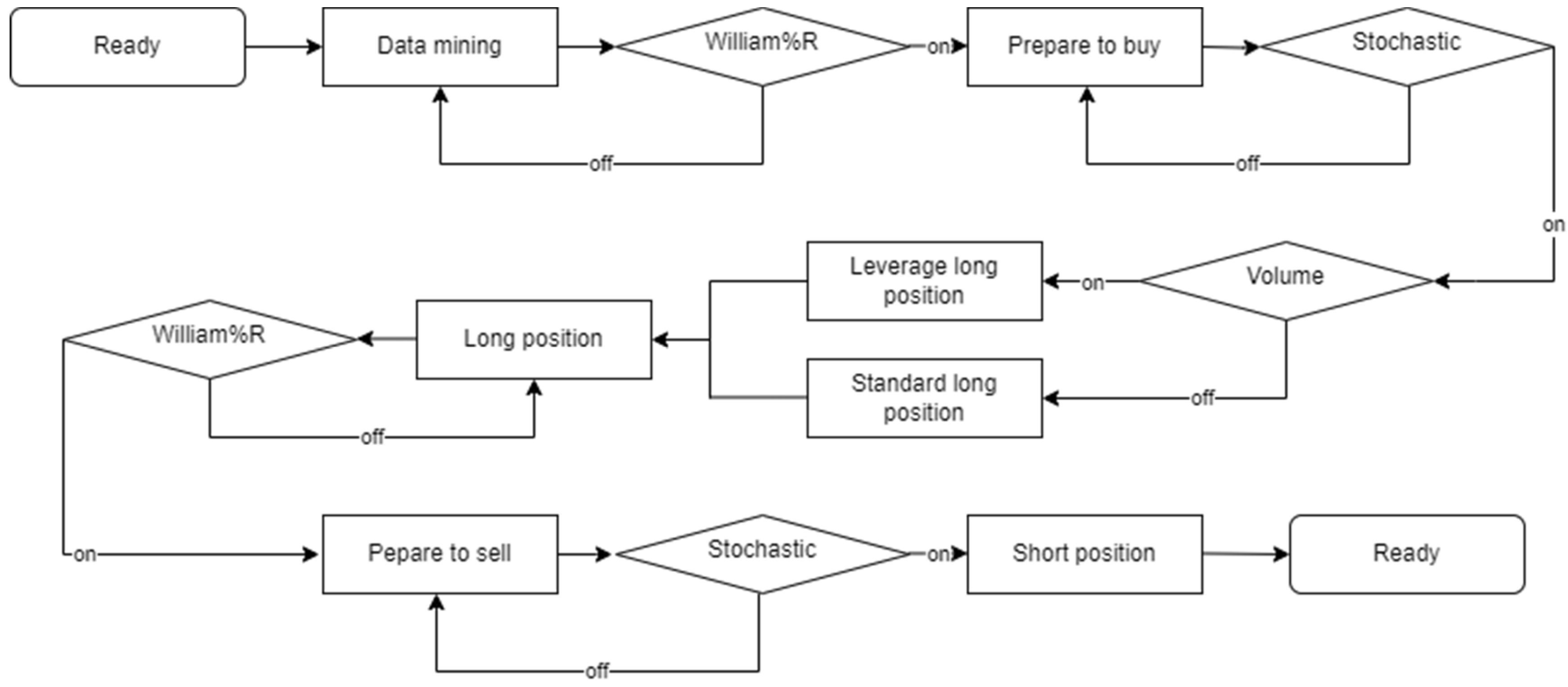
Figure 2.
SPY ETF’s combined William%R and stochastic oscillator trends.
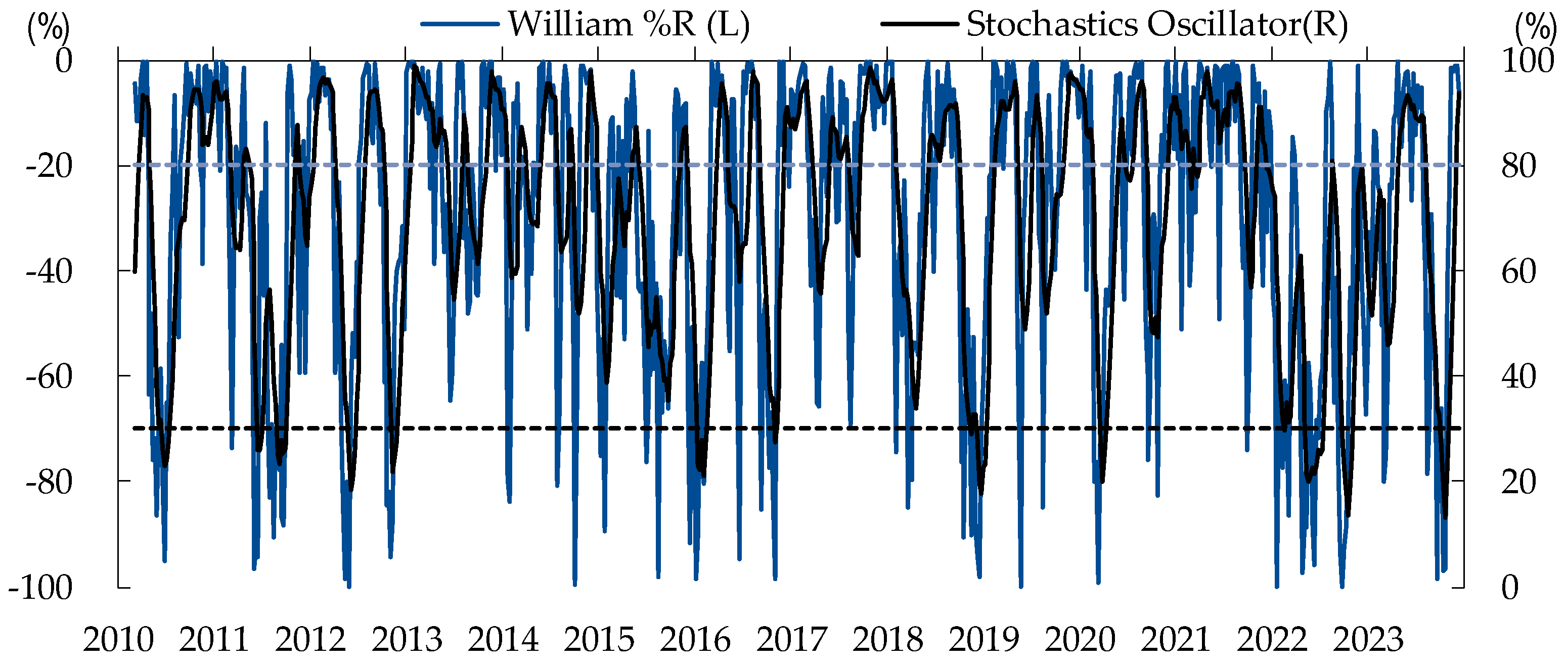
Figure 3.
SPY ETF’s separate William%R and stochastic oscillator trends.
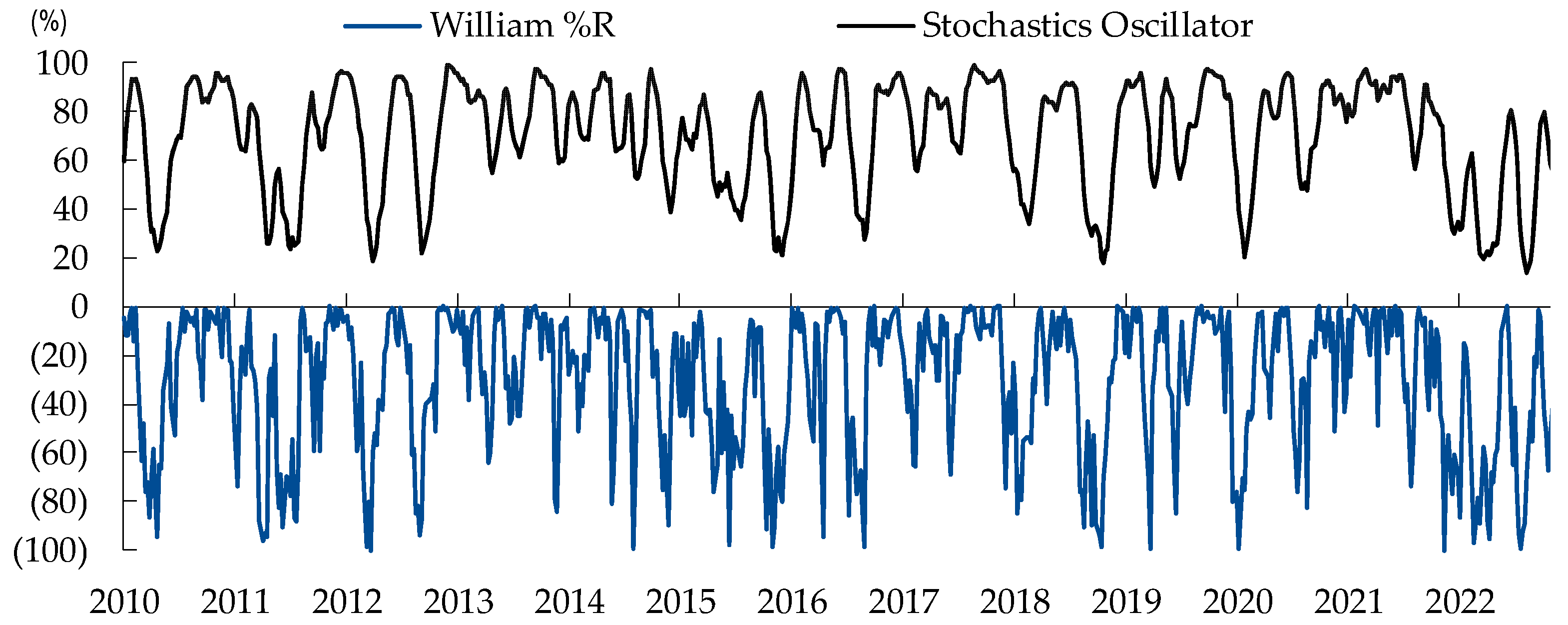
Figure 4.
SPY ETF’s buy and sell signals according to the algorithm. Black arrows indicate a buy signal, and blue arrows indicate a sell signal. Ten trading signals were generated (buy and sell).
Figure 4.
SPY ETF’s buy and sell signals according to the algorithm. Black arrows indicate a buy signal, and blue arrows indicate a sell signal. Ten trading signals were generated (buy and sell).
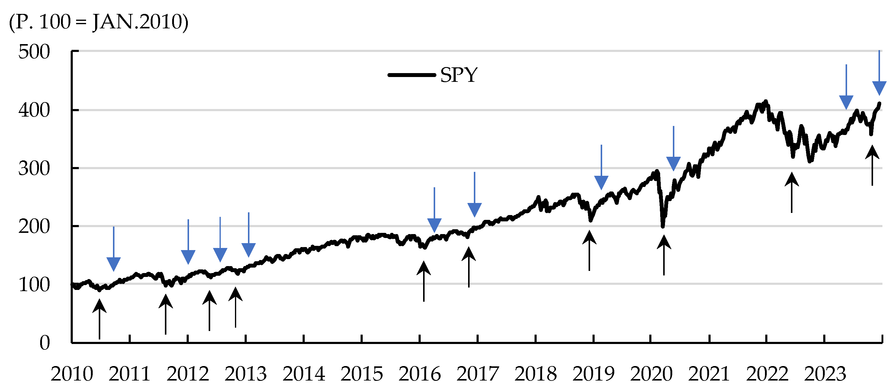
Figure 5.
SPY ETF’s price and volume trends.
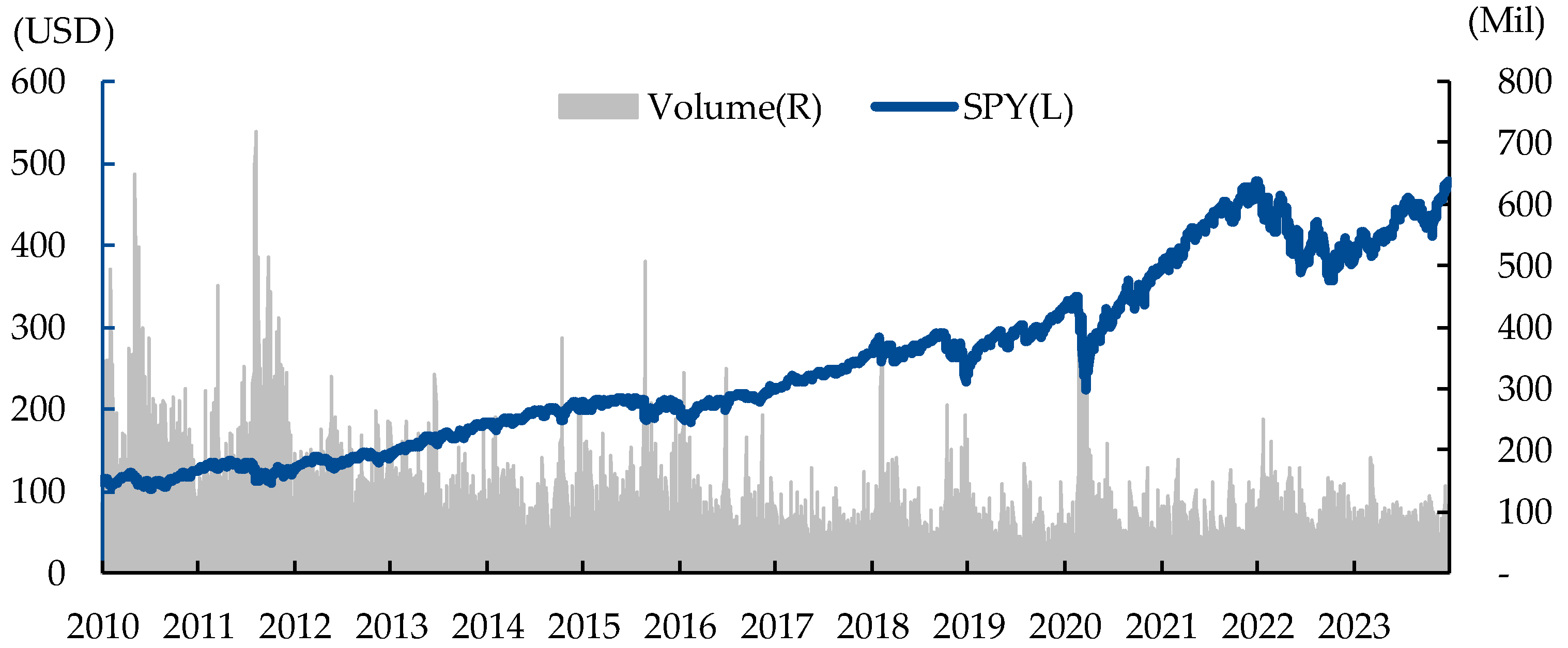
Figure 6.
SPY ETF’s one-year average volume and volume trends.
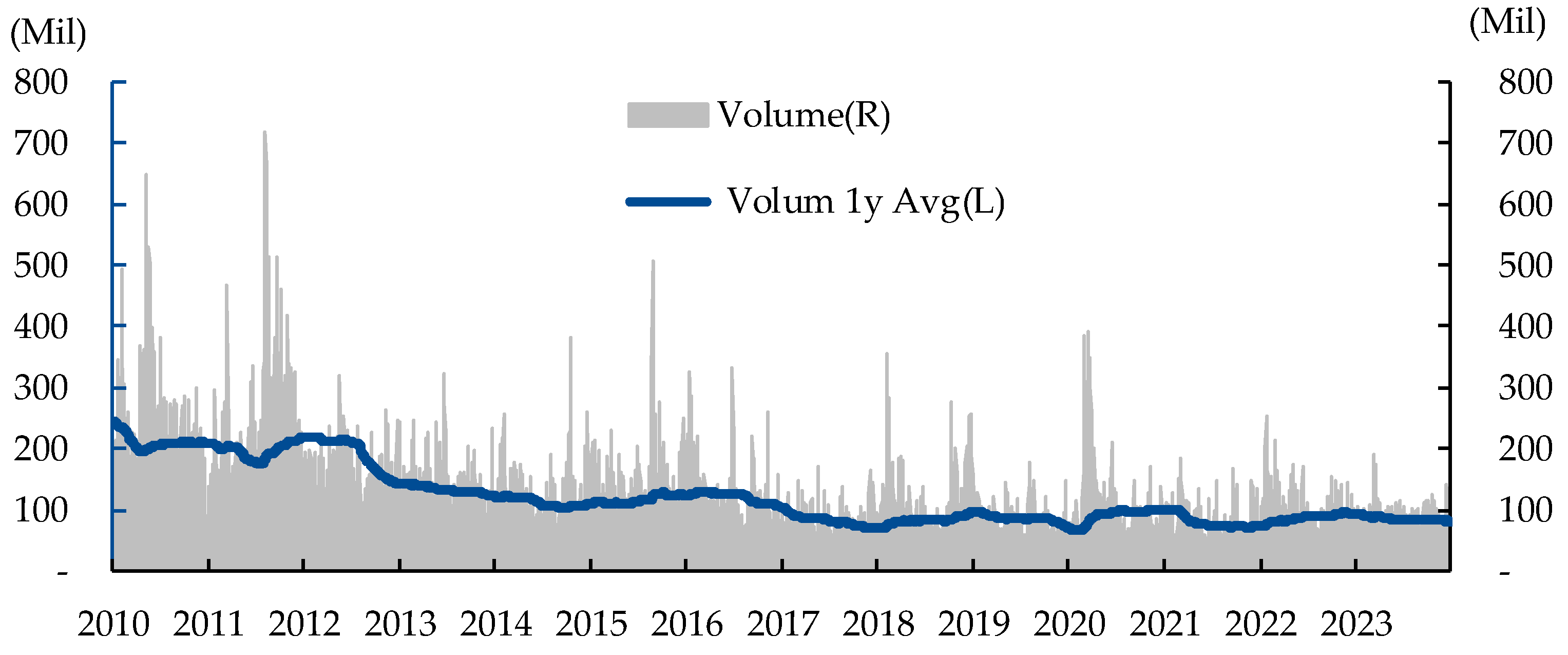
Figure 7.
SPY ETF’s one-year average volume plus one standard deviation, one-year average volume, and volume trends.
Figure 7.
SPY ETF’s one-year average volume plus one standard deviation, one-year average volume, and volume trends.
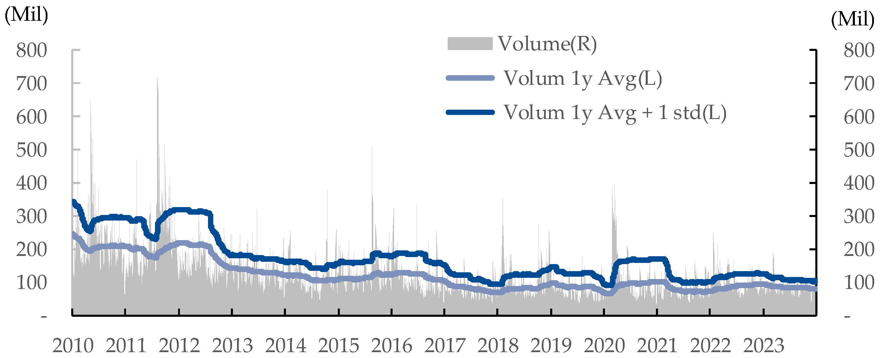
Figure 8.
SPY ETF trend, standard (×1) trading trend.
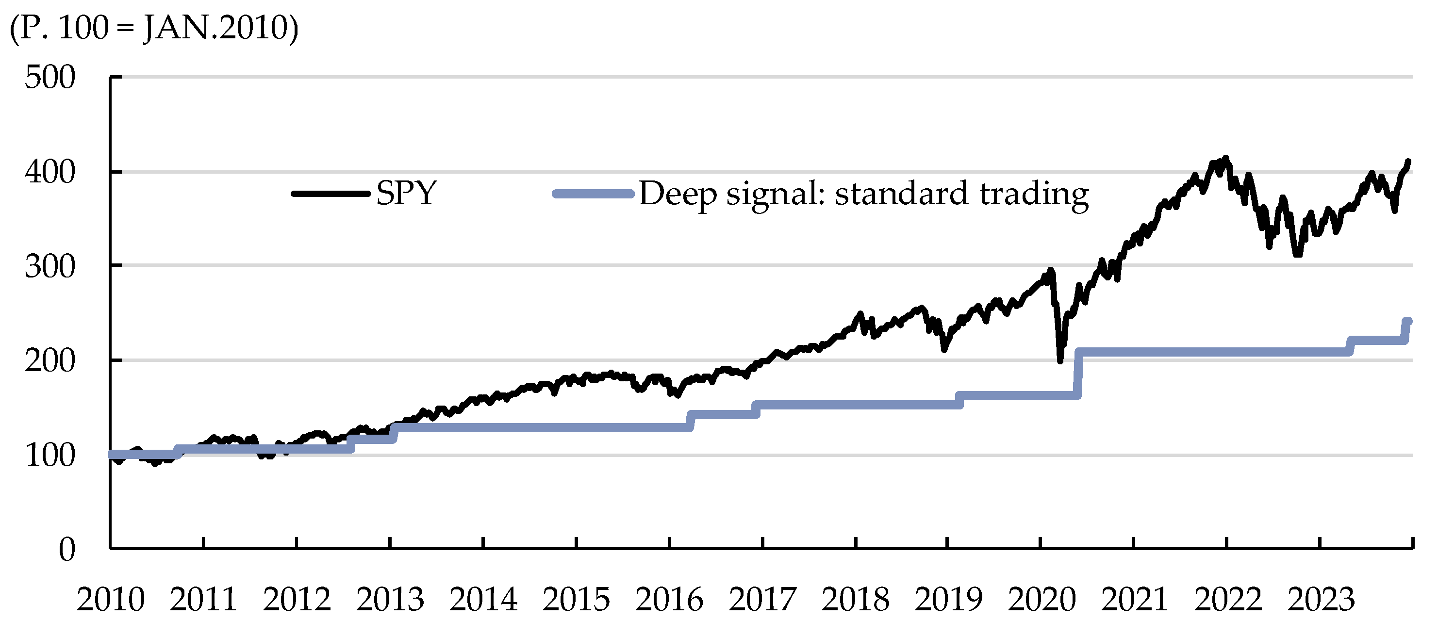
Figure 9.
SPY ETF trend, leverage trading trend.
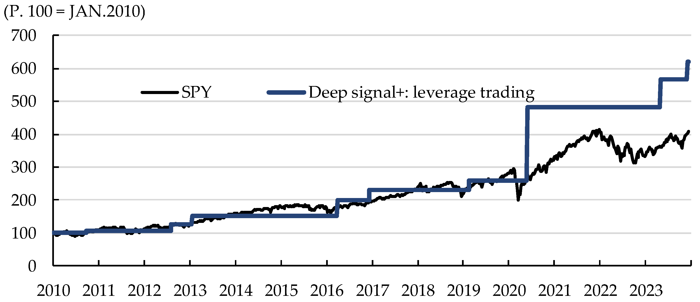
Figure 10.
SPY ETF trend, leverage trading trend.
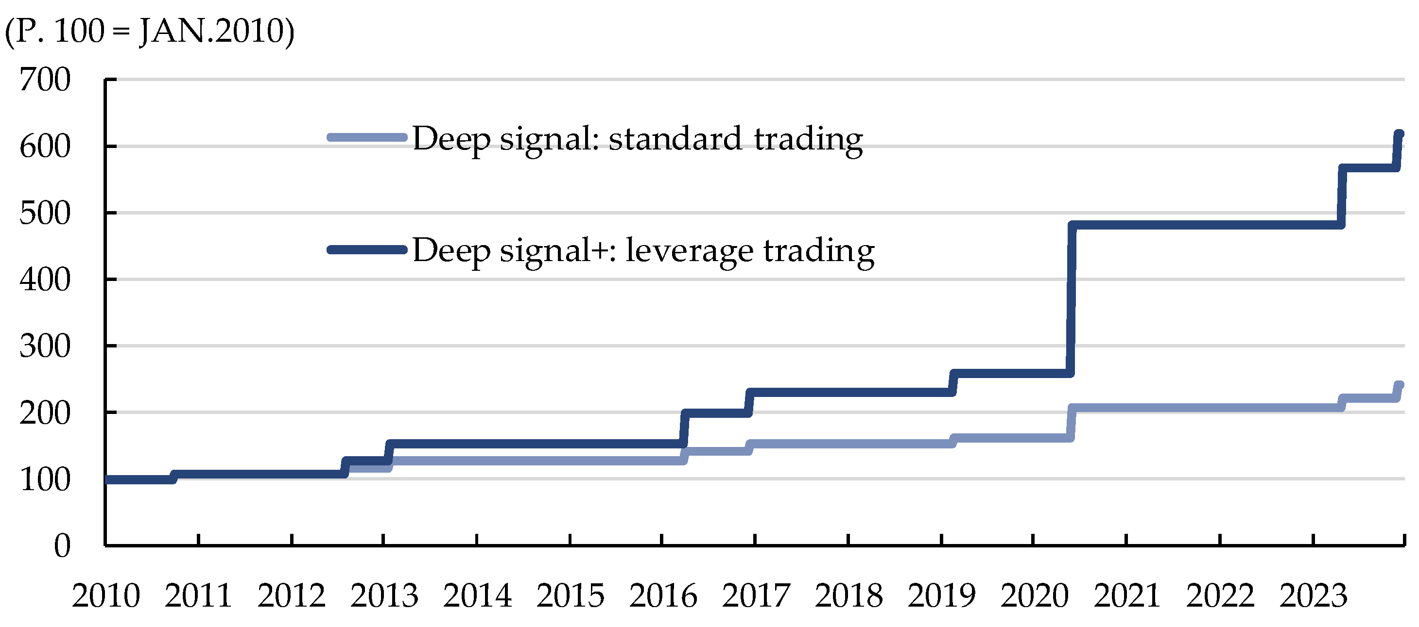

Table 1.
The core measurement numbers of SPY ETF algorithm trading.
| index | SPY results | |
|---|---|---|
| period | Jan.2010 ~ Dec.2023 | |
| trading numbers | 10 | |
| numbers of gain | 9 | |
| numbers of lose | 1 | |
| hit-ratio(%) | 90.0 | |
| DeepSiganl Model standard trading (x1) |
max drawdown(%) | -0.1 |
| max gain(%) | 28.7 | |
| total return(%) | 141.2 | |
| Annr(%) | 7.0 | |
| ARM ratio(%) | 70.0 | |
| PARC(%) | 0.07 | |
| DeepSignal+ Model leverage trading |
max drawdown(%) | -0.2 |
| max gain(%) | 86.0 | |
| total return(%) | 519.3 | |
| Annr(%) | 15.1 | |
| ARM ratio(%) | 75.5 | |
| PARC(%) | 0.151 | |
| S&P 500 index |
max drawdown(%) | -15.1 |
| max gain(%) | 12.1 | |
| total return(%) | 375.0 | |
| Annr(%) | 11.6 | |
| ARM ratio(%) | 0.768 | |
| PARC(%) | 0.098 | |
* Maximum drawdown is based on the weekly negative change rate; maximum gain is based on the weakly positive change rate; AnnR = end price/start price; ARM ratio = AnnR/MaxD; PARC = AnnR × (1 − MaxD).
Table 2.
A DeepSignal simulation trading table of the SPY (S&P 500) ETF.
| Date | SPY * | DeepSignal | Buy/Sell | Return Rate |
Stochastic | William%R |
|---|---|---|---|---|---|---|
| 4-Jan-10 | 114.6 | 100.0 | Start | |||
| 21-Jun-10 | 107.9 | 100.0 | BUY | 26.1 | −80.3 | |
| 27-Sep-10 | 114.6 | 106.2 | SELL | 6.2 | 82.3 | −10.3 |
| 20-Jun-11 | 126.8 | 106.2 | BUY | 26.0 | −94.4 | |
| 7-Nov-11 | 126.7 | 106.1 | SELL | −0.1 | 82.4 | −12.6 |
| 28-May-12 | 128.2 | 106.1 | BUY | 24.7 | −100.0 | |
| 6-Aug-12 | 140.8 | 116.6 | SELL | 9.9 | 86.1 | −0.6 |
| 12-Nov-12 | 136.4 | 116.6 | BUY | 22.0 | −87.5 | |
| 21-Jan-13 | 150.3 | 128.5 | SELL | 10.2 | 85.6 | 0.0 |
| 11-Jan-16 | 187.8 | 128.5 | BUY | 23.2 | −91.0 | |
| 28-Mar-16 | 206.9 | 141.6 | SELL | 10.2 | 85.3 | −0.8 |
| 31-Oct-16 | 208.6 | 141.6 | BUY | 27.6 | −98.4 | |
| 12-Dec-16 | 225.0 | 152.8 | SELL | 7.9 | 89.0 | −16.5 |
| 19-Nov-18 | 263.3 | 152.8 | BUY | 28.9 | −90.0 | |
| 18-Feb-19 | 279.1 | 162.0 | SELL | 6.0 | 82.5 | −0.5 |
| 30-Mar-20 | 248.2 | 162.0 | BUY | 20.1 | −75.2 | |
| 1-Jun-20 | 319.3 | 208.4 | SELL | 28.7 | 85.7 | −2.5 |
| 16-May-22 | 389.6 | 208.4 | BUY | 21.5 | −88.9 | |
| 1-May-23 | 412.6 | 220.7 | SELL | 5.9 | 86.2 | -13.5 |
| 16-Oct-23 | 421.2 | 220.7 | BUY | 19.3 | -97.0 | |
| 4-Dec-23 | 460.2 | 241.2 | SELL | 9.3 | 87.7 | -1.1 |
| 25-Dec-23 | 475.3 | 241.2 | End |
* The primary ETF price data from the Yahoo finance site.
Table 3.
A DeepSignal+ simulation trading table of the SPY (S&P 500) ETF.
| Date | SPY * | Deep Signal+ |
Stochastic | William%R | Buy/Sell | Return Rate |
Volume (k) |
52w AVG Volume(k) |
52w +1std(k) |
|---|---|---|---|---|---|---|---|---|---|
| 4-Jan-10 | 114.6 | 100.0 | Start | ||||||
| 21-Jun-10 | 107.9 | 100.0 | 26.1 | −80.3 | BUY | 213,140.7 | 204,608.1 | 84,282.4 | |
| 27-Sep-10 | 114.6 | 106.2 | 82.3 | −10.3 | SELL | 6.2 | |||
| 20-Jun-11 | 126.8 | 106.2 | 26.0 | −94.4 | BUY | 159,479.0 | 179,370.8 | 60,152.6 | |
| 7-Nov-11 | 126.7 | 106.0 | 82.4 | −12.6 | SELL | -0.2 | |||
| 28-May-12 | 128.2 | 106.0 | 24.7 | −100.0 | BUY | 152,883.5 | 214,504.6 | 99,797.0 | |
| 6-Aug-12 | 140.8 | 127.0 | 86.1 | −0.6 | SELL | 19.8 | |||
| 12-Nov-12 | 136.4 | 127.0 | 22.0 | −87.5 | BUY | 97,677.5 | 150,794.1 | 45,951.9 | |
| 21-Jan-13 | 150.3 | 152.8 | 85.6 | 0.0 | SELL | 20.4 | |||
| 11-Jan-16 | 187.8 | 152.8 | 23.2 | −91.0 | BUY | 187,941.3 | 124,275.5 | 55,937.7 | |
| 28-Mar-16 | 206.9 | 199.5 | 85.3 | −0.8 | SELL | 30.5 | |||
| 31-Oct-16 | 208.6 | 199.5 | 27.6 | −98.4 | BUY | 61,272.5 | 108,508.7 | 48,956.4 | |
| 12-Dec-16 | 225.0 | 231.0 | 89.0 | −16.5 | SELL | 15.8 | |||
| 19-Nov-18 | 263.3 | 231.0 | 28.9 | −90.0 | BUY | 103,061.7 | 90,593.1 | 45,031.4 | |
| 18-Feb-19 | 279.1 | 258.9 | 82.5 | −0.5 | SELL | 12.1 | |||
| 30-Mar-20 | 248.2 | 258.9 | 20.1 | −75.2 | BUY | 171,369.5 | 86,450.7 | 68,913.9 | |
| 1-Jun-20 | 319.3 | 481.6 | 85.7 | −2.5 | SELL | 86.0 | |||
| 16-May-22 | 389.6 | 481.6 | 21.5 | −88.9 | BUY | 78,622.4 | 85,514.8 | 36,783.2 | |
| 1-May-23 | 412.6 | 566.8 | 86.2 | -13.5 | SELL | 17.7 | |||
| 16-Oct-23 | 421.2 | 566.8 | 19.3 | -97.0 | BUY | 75,433.2 | 82,986.7 | 21,914.7 | |
| 4-Dec-23 | 460.2 | 619.3 | 87.7 | -1.1 | SELL | 9.3 | 159,479.0 | 179,370.8 | 60,152.6 |
| 25-Dec-23 | 475.3 | 619.3 | End |
* The primary ETF price data from the Yahoo finance site.
Disclaimer/Publisher’s Note: The statements, opinions and data contained in all publications are solely those of the individual author(s) and contributor(s) and not of MDPI and/or the editor(s). MDPI and/or the editor(s) disclaim responsibility for any injury to people or property resulting from any ideas, methods, instructions or products referred to in the content. |
© 2024 by the authors. Licensee MDPI, Basel, Switzerland. This article is an open access article distributed under the terms and conditions of the Creative Commons Attribution (CC BY) license (http://creativecommons.org/licenses/by/4.0/).
Copyright: This open access article is published under a Creative Commons CC BY 4.0 license, which permit the free download, distribution, and reuse, provided that the author and preprint are cited in any reuse.


