
Submitted:
04 November 2025
Posted:
05 November 2025
You are already at the latest version
Abstract
This study conducts experimental and modeling analyses to comprehend the unsteady flow phenomena within cavity gaps, with a specific focus on finding the optimal rim seal flow rate for enhancing turbine efficiency. The rim seal flow phenomenon is investigated and validated against the University of BATH's single-stage turbine experiment rig. The emphasis is on the steady-state computation of rim seal qualities using passive-scalar transport for tracer gas modeling, with limited exploration of unsteady phenomena. The LISA 1.5 stage model from Zurich University serves as a baseline for turbine efficiency studies, incorporating the rim seal configuration. The computational domain's influence, including the turbomachinery Multi-Reference Frame approach, is investigated. While the Frozen Rotor accurately predicts ingression flow fields, the no-interface model poorly predicts ingression, favoring a simplified "thin seal" model. A statistical approach is introduced for the "Orifice" model to implicitly calculate the minimum sealing flow for each rim seal configuration. Pre-swirling the rim seal demonstrates a reduction in shear forces on the rotor wall, consequently lowering friction torque on the rotor disc. However, swirling flow appears ineffective in influencing ingression and egression due to the model's long propagate distance. In addition to steady-state investigations, the harmonic balance method explores unsteady phenomena in Axial turbine configuration. Kelvin-Helmholtz instabilities within the rim seal gap are observed, acting as driving mechanisms for large-scale structures at 98% rotor speed. Incorporating wheel-space cavities in the LISA 1-stage model significantly alters flow phenomena and turbine efficiency. Rotor-stator interaction at specific times can complicate wheel space sealing, contrary to bladeless model predictions. Furthermore, an increase in rim seal flow is associated with reduced turbine isentropic efficiency.
Keywords:
single-stage axial turbine
; rim seal
; RANS analysis
; Kelvin-Helmholtz instabilities
; ingression
; turbine efficiency
1. Introduction
The efficiency of a turbine is measured by its aerodynamic performance, which compares the actual work generated to theoretical calculation. Adiabatic efficiency is the most common definition of efficiency for turbines, and it’s determined by comparing the actual work of the turbine to the theoretical isentropic work. When high enthalpy fluid enters the turbine, it’s converted into shaft power due to expansion and accelerated flow. The stage degree of reaction measures the ratio of the static enthalpy drop in the rotor to the enthalpy drop in the entire stage. The degree of reaction splits the rotor into two sides: the Reaction turbine where the degree of reaction is 1 and an impulse turbine where the degree of reaction is 0. The main difference between these two types of turbines is the pressure field across the stage. For the impulse turbine, the static pressure remains un-changed, while the reaction uses the pressure drop to create a reaction force. Adiabatic efficiency and degree of re-action determine the turbine configuration.
The losses in a turbine can be explained by the generation of entropy during the process. This can be due to the increase in entropy of the fluid or the waste of energy. Den-ton [1] identified two aerodynamic processes that lead to entropy generation: viscous friction in the boundary layers or free shear layers, and the mixing process of fluids, such as coolant flow. Heat transfer problems between different temperatures, such as the mainstream flow and coolant flow, also contribute to the loss. In turbines, viscous effect and non-equilibrium processes play a major role in entropy generation. Cavity flow to the mainstream passage is a specialty in this study, but the leakage loss [2] and the secondary or end wall losses [3,4,5,6] are among the majority losses of the turbine stage. These losses are caused by complex 3-dimensional flow phenomena resulting from the rapid com-plex mixing between fluids. The thickness of the inlet boundary layer [7,8] and the turning of the blade are also important factors that lead to the end wall loss. Using the numerical method, Dawes [9] stated that 90% of entropy generation occurs within the edge of the logarithmic zone (y+ ~30), where the velocity and temperature gradients are greatest. Dawes also noted that the passage vortex sucks the fluid out from the boundary layer and mixing with the mainstream flow, makes the downstream boundary layer thinner. Moreover, the secondary vortex attaches to the suction surface, creating high shear stress and high turbulent intensity across the blade. As a result, at the local region above the trailing edge end-wall exhibit a very high entropy fluid. The turbine is cooled by coolant fluid that bleeds from the compressor. Denton [1] stated that the entry of the cooling fluid removes the heat from the system, decreasing the entropy, thus enhances the turbine stage’s efficiency. However, the mixing process between the coolant and mainstream fluids causes an irreversible entropy increased effect in the local region. According to Shapiro [10], mixing loses depend on the stagnation pressure, temperature, mass flow rate, and the angle between two fluid streams. The worst case is when cosine is equal to 0 (90 degrees) creating the most mixing between the two fluid streams, leading to maximum missing losses. With the injection of cooling fluid, the blockage effect will enhance the end-wall losses by obstructing the flow in the mainstream [11]. As the turbine disc rotates in a stationary fluid, the centrifugal force creates a radial flow, which is offset by an axial flow [12,13,14]. With the turbine stationary and the fluid rotating, the back pressure gradient pushes the fluid toward the center [15]. The combination of a stationary and rotating disc creates a wheel-space cavity with fluid movement [16,17]. The flow structure inside the wheel space of the rotor-stator system is dependent on the on the geometry of the gap [18,19,20] and Rotational Reynolds number (Reϕ) [21]. Despite their significant contribution to losses, end-wall losses have not been fully described from a physical point of view and still depend on empirical performance.
In the context of gas turbine engineering, these are two major phenomena that induce the penetration of hot gases into the cavities, the rotationally induced ingress (RI) is caused by the motion of the rotor disc, and externally induced ingress (EI) is caused by the non-axisymmetric flow structure in the mainstream. In studies [22,23,24,25], it was emphasized that the roles of pressure, the rim-seal geometry, rotational Reynolds number and provided experimental and modeling methods for evaluating and controlling the rotationally induced ingress. Experiments showed that minimum sealing flow is influenced by geometry and Reynolds number [22], and radial seals are more effective than axial seals [23]. Unlike rotational ingress, the externally induced ingress does not depend much on the rotational Reynolds number. An experiment conducted in [26] showed that ingression can be influenced by the disturbance of the annulus. The importance of pressure gradients in the anulus, which can dominate the rotational Reynolds number was highlighted. Phake and Owen [27,28] upgraded their previous experimental rig to simulate the non-asymmetric pressure in the mainstream annulus. Both types of ingressions were observed and separated into two regimes, and the correlation between the two regimes can be expressed by the ratio of the mainstream Reynolds number and the Rotational Reynolds number. They also presented an empirical model to calculate the minimum flow rate re-quired for sealing, emphasizing the role of pressure in the EI phenomenon. The influence of mainstream flow disturbances and blade geometry on EI have been investigated in studies [29,30,31,32,33]. The presence of blades increased the circumference pressure distribution downstream of the vanes. The sealing effectiveness across the radial direction of the stator wall was also measured. Both CFD and experimental results agreed that the ingression zone at the rim seal gaps moves at half the speed of the rotor. Most recently, Sangan et al. [34,35] at the University of BATH conducted a single-stage turbine that can operate to a Rotational Reynolds number of nearly 1 million. Forming 32 stator vanes and using a NACA aero foil as a rotor blade, combined with concentration measurement and pressure tap to determine the sealing effectiveness and pressure distribution at the mainstream flow. The author also introduces a new non-dimension parameter that includes the geometry of the rim seal, the seal-ant rate, and the rotation speed. This new parameter is especially helpful for scaling the flow from the test rig to the real engine condition [36] by developing a theoretical function that will be discussed under. And most importantly, in this study will be using the stator vane model drive from this experiment. In summarize, the rotational induced ingress (RI) is the resultant of the rotor-stator system. With a fully sealed cavities got the rotating core suppressed. The pressure driven ingress (EI) prevails over the counterpart in most gas turbines engine, resulting from the unsteady flow behind the structure of the mainstream cause the pressure to be quasi-axisymmetric.
For a wide range of experiments and CFD studies the phenomena of the rim seal over the years, numerous studies have found the instability that occurred at a frequency that unrelated to the rotor speed as another key driven of ingression. Teuber et al. [36] investigated the wheel space within a rotating frame of reference using the BATH rig model, conducting both steady and unsteady computations. They found that the Multi Reference Frame (MRF) method significantly influenced the level of ingression, outperforming unsteady RANS in computational efficiency and predicting rim seal flow quality and quantity. Rotor blades had minimal impact on pressure distribution at the stator’s trailing edge. Mirza Moghadam et al. [37] studied steady RANS with a full-stage turbine, submerging the cavity in the stationary domain to eliminate rotor blade interaction via a mixing plane interface. They observed seal mixing efficiency and noted that the stator hub fillet improved sealing effective-ness, with stator wake exerting more influence on ingression than rotor wake. Liu et al. [38] conducted multiple do-main experiments on the BATH test rig, comparing results with previous studies. They found discrepancies in pressure distribution between bladeless RANS and URANS, with RANS overpredicting peak pressures but displaying faster pressure decay downstream. RANS failed to accurately predict flow near rim seal gaps due to high unsteadiness. Sealing effectiveness predictions were poor in both wheel-space domains, though non-inertia frame wheel space yielded better agreement with experimental data. Authors suggested investigating MRF interface location for optimal mainstream swirl. Rotor blades in URANS had little influence on upstream flow compared to test rig purposes. Rabs et al. [39] examined rim seal flow instabilities based on free shear flow phenomena. They described Helmholtz instabilities arising from velocity differences in parallel flows, causing vortices that disrupt flow dynamics near rim seal gaps and potentially affect ingress and mainstream flow mixing. These instabilities form a traveling wave within the rim seal gap, influencing sealing flow rate and interaction between vanes and blades. Beard et al. [40] conducted experiments on a wheel space-only rig operating at higher rotational speeds, observing less large-scale structure and increased sealing flow, with structure velocity remaining constant around 80%. Gao et al. [41] used Large-Eddy Simulation (LES) for the same rig, finding significantly more large-scale structures than experimental data, moving at 43% of rotor speed. They observed a gap recirculating zone (GRZ) vortex structure, suggesting another mode of instabilities that disappeared at high sealing flow rates. Furthermore, Gao et al. [42] observed Taylor-Couette Vortex instabilities in chute seals, with recirculation disappearing at high sealing flow rates. They noted high vorticity at stator or rotor walls, indicating Taylor vortex presence and its potential impact on seal configuration. Through LES investigation, Gao et al. [43] confirmed the presence of inertial waves, showing velocity fluctuations in phase with each other but out of phase with the pressure field, satisfying the momentum equation. They concluded that ingress and egression interference through rim seal gaps complicates flow prediction, marking a new understanding of rim seal flow structure. In summarize, the Multi Reference Frame gives the best result for a steady RANS simulation of the rim seal flow with the wheel-space submerged inside the relative frame. For an Un-steady RANS, the number of the passage per domain will influence the flow structure due to the present of the large-scale structure inside the wheel-space. Large-Eddy Simulation undertook for both full domain and simplified domain encounter the instabilities such as Kelvin-Helmholtz, Taylor Vortex…suggested to be the driven forced of the large-scale structure fluctuation within the rim seal gap.
For CFD applications, the influence of computational domain plays a significant role in the ingression and sealing effectiveness measurement. While RANS adoption shows fast and reliable computation the rim seal phenomenon but still cannot give the real insight into the already unsteady flow structure. Unsteady simulations give the insight of the flow field but are usually found to be computationally ex-pensive. The reduction of computational domain might give different large-scale structures. In the scope of this study, the harmonic balance method based on frequency domain is adopted to have the first of understanding the unsteady of the rim seal flow.
2. Geometry
2.1. Description of LISA Geometry
The turbine test facilities “LISA” at Turbomachinery Laboratory of ETH Zurich built by Behr [2] is an axial flow, low-temperature, subsonic, staggered turbine. As illustrated in Figure 1, the turbine test rig is designed to operate in a loop that opens to the ambient atmosphere. Constructed with 2 stators and 1 rotor with an addiction stator at inlet and outlet to straight out the flow making it a 1.5 stage turbine. With the maximum limits of the turbine including the expansion ratio of 1.5 and mass flow rate of 13 kg/s creating it a high-pressure turbine. Despite being a testing rig with far form realistic gas turbine, but still give LISA excellent reputation in the illustrator of the turbine phenomenon. Providing a wide range of experiment data, LISA turbine is the best suited to simulate the turbine flow philosophy. In this study, for investigating the influence of the rim seal cooling flow, a 1-stage LISA adapted from the 1.5 stages is used.
2.2. Review of BATH Cavities Experimental Rig
In this study, thanks to Sagan [31] at mechanical engineering department of University of BATH to provide public data on the experiment, conducting the computational do-main based on the experiment rig. The domain is constructed of stationery, non-staggered, 560 turning vanes and 32 NACA 0018 rotor blade. Concentration measurements inside the wheel space are used to calculate the sealing effectiveness. Static pressure tap is located at stator wall along with pitot tubes. The rim seal geometry in this thesis is based on the rim seal geometry of the BATH test rig also. With the configuration denoted Gen#1, #2 and #4 is taken into consideration. The BATH test rig is designed to rotate at a maximum speed of 4000 RPM, with the publication data including 2000, 3000 and 3500 RPM. In this study, only the 3500 RPM cased is used.
Figure 2 is a meridional view sketch of Gen #1 computational domain used. With annulus pressure measurement located Point A 2mm upstream from the rim seal edge. Sealing effectiveness measurements main data is located at non-dimensional radius r/ro = 0.958. Other miscellaneous fluid properties reference measurements like density, viscosity, etc. are located at r/ro = 0.993. The pitot tube for swirling flow measurements is located at the non-dimensional axial wheel space location of z/s = 0.25 (0 for the stator and 1 for the rotor).
In the experiments, the test rig using ambient air, laboratory conditions of 250 Celsius flow through a venturi tube at the inlet to measure the mass flow rate. The outlet flows to a volute and dumps into ambient atmosphere. To demonstrate in numerical simulations, inlet mass flow rate and pressure outlet are used with the turbulent intensity of 5%. Moreover, the sealing flow inlet in the experimental does not contain a pre-swirl nozzle for adding the rotation speed to the fluid. So, in this study, using boundary conditions can investigate both pre-swirl and non-pre-swirl cases. The pre-swirl can give the flow easier to match the spinning boundary layer on the rotor.
3. Numerical Method
3.1. Numerical and Harmonic Balance Approach
In this study, ANSYS CFX 2024 R2 was employed to solve the governing differential equations, including the continuity, Reynolds-averaged Navier-Stokes (RANS), and energy equations. CFX utilizes the finite method, which is based on an underlying finite element mesh. The spatial domain is first discretized into a mesh, from which finite volumes are constructed. Conservation laws for mass, momentum, and energy are then applied to each finite control to perform the calculations. The Shear Stress Transport based on the k−ω turbulence model is used in the validation process as it previously proves giving the best result [40÷42]. The convergence criteria are established such that the root-mean-square values for continuity, momentum, energy, turbulent kinetic energy, and specific turbulent dissipation rate are all below 1×10⁻⁴. In addition, to ensure the results of interested parameter monitored to absolutely converge. The multi reference frame (MRF) method is also used in this thesis to simulate the rotational blades. The “rotation domain” or the no inertia domain adds the tangential velocity directly to the source term of the momentum equation. Incorporating the changing interface used both Stage (Mixing-plane) and Frozen Rotor to evaluate the influence of the interface. For reduced computational resource, the size of the domain only incorporates a single passage, connected circumferentially by the rotational periodicity with GGI interface. To accommodate the tracer gas in the simulation, a passive-scalar is used to represent the transportation of the multi-gasses’ domain. An active scalar is an actual gas that has all the molecular properties and the reaction with regular air in the domain. In contrast, the passive scalar is used just for modeling the transport equation and is not heavily involved in the main fluid flow physics. This simplified the computational resources but still gives the accurate result for a tracer gas. To portrait as close as possible to the experiment, the kinematic diffusive coefficient (m2/s) is set for CO2 in the passive scalar. The diffusive coefficient represents how the fluids expended in space correlated with temperature, this coefficient can be obtained from experimental or using Chapman-Enskog theory with 8% error. For this study, a small range of temperature is used so it is benefit from using the experimental results. In every turbomachinery involving a couple of vanes and blade, exhibiting both of spatial and temporal periodic in turbomachinery, harmonic oscillations based on the fundamental frequency of the Blade Passing Frequency (BPF) or the rotor rotation speed. This behavior leads to the adoption of a frequency-domain approach to address the problem. In the Harmonic Balance method, the governing Navier-Stokes equations are transformed using a Fourier series in time, while incorporating coefficients that vary spatially. The harmonic balance method solving multiple steady state solution at difference blade angle (time plane) to archive the Fourier series for the unsteady behavior of the flow field. In this study, the Harmonic Balance method will be applied to the BATH test rig case.
3.2. Computational Domain and Theoretical Basis
3.2.1. LISA 1.5 Stage Turbine
The computational domain is conducted based on Behr experimental rig, with 36 stator vanes for S1 and S2 (stator 1 and stator 2) and 54 blades (R1). Illustrated in Figure 3, the inner hub has a radius of 330mm, and the outer shroud is 400mm. Since the tip geometry is not provided, the tip clearance is set to 1% of the blade span, matching the test rig configuration. With only one passage considered and the side surface set as a rotational periodicity interface type, with the mesh connection type selected “GGI” method. The geometry of the blades and vanes including the computational domain is constructed in CATIA and imported to the meshing application. A very important side note here is that the experiment is a 1.5 stage turbine, however, in the scope of this thesis, only 1 stage turbine is needed. That is why the author of this study calculates the problem a little bit explicitly here. Accessor to Chung [48] previous data on the LISA 1.5 stage, using nearly the same equal amount of mesh and the same domain to achieve the flow field solution. Then, using the result output as the boundary conditions for the 1 stage turbine. This approach greatly reduces computational resources but still results in great quality and quantity; the result will be discussed in the next chapter.
One thing to note for the domain considerations is the traverse plane that is used to measure experiments. Illustrated in Figure 3, the measured plane shows the position of the interface located at the traverse plane for easier measurement. And the numbering of the plane is convenient for the calculation formular subscript. However, for the rim seal add-in configuration, the traverse plane is located between vanes leading edge and blades trailing edge stay above the rim seal clearance, making it impossible to place the interface above. So, to overcome that, the domain interface is moved upstream 2 mm. This is also a convenience as the wheel-space can be submerged inside the rotating domain. The inlet is moved far away upstream two times S1 axial chord from S1 leading edge for a fully developed flow; and the outlet is moved downstream two times S2 axial chord from S2 trailing edge to avoid outlet boundary conditions error.

Table 1.
Measurement Plane and Position.
| Plane | Relative position | Location measurement |
| 1 | Upstream S1 | 40% S1 Axial Chord |
| 2 | Downstream S1 | 15% S1 Axial Chord |
| 3 | Downstream R1 | 15% R1 Axial Chord |
| 4 | Downstream S2 | 15% S2 Axial Chord |
The domain is discretized (meshed) for both the 1.5-stage turbine and the 1-stage configuration. The mesh using here is structured grid, hexahedral—shaped mesh, with mesh number of the 1.5 stage (Figure 4 and Figure 5) calculated already refined about 6.0 million mesh and for the 1 stage, 3 meshed varied from 9.5 hundred thousand to 5.7 million will be considered for the numerical derivative. The mesh elements adjacent to the rotor and rim seal walls are specified with a height of 3×10⁻⁶ meters to accurately resolve the boundary layers within the viscous sublayer region. This setup uses the k-ω SST turbulence model combined with the Kato-Launder limiter.
For validation purposes, the reliability of the numerical method, the result from CFD will be compared with the experiment test rig through non-dimensional fluid dynamics variables that commonly seen in turbomachinery.
The total-to-total efficiency of the turbine with a fitted rim seal, adapted from [43]:
This new equation is considered the addition of rim seal flow total enthalpy into the expansion cycle. The added variable here is the total pressure measured at the inner cavities pt,cav. In the experiment conducted by [43]) at ETH, static pressure within the cavities was measured at the stator wall, well away from the rim seal clearance. Meanwhile, velocity through the rim seal gap was measured in the drum beneath the wheel space, close to the inner seal. Thus, in a different rim seal geometry, the place to measure the pressure might be arbitrary. However, in a later modified experimental test rig at ETH, [44] can put the measurement probe deep into the rim seal gap to show a better output. In conclusion, it is most effective to measure pressure at the inner rim seal or near the disk radius’s end, where the flow does not penetrate the outer rim seal.
The degree of reaction, where “h” is the static enthalpy:
Pressure expansion: total-to-static for 1.5 stage, total-to-total for 1 stage.
The flow coefficient is the ratio of axial velocity through the rotor to the blade speed.
The loading coefficient represents the actual work done by the blade with the blade speed:
The pressure coefficient for both total and static is defined as:
The total pressure loss coefficient represents the total pressure drop across the vane or blade row normalized by the dynamic head at the vane or blade exit, used to quantify secondary losses.
3.2.2. BATH Cavities Experimental Rig
The domain used here contains a single passage to represent 32 vanes like the LISA approach. The Stator vanes domain was constructed with the stator inlet extended about 2 times stator axial chords for a fully developed flow. Figure 6 shows the projection view of stator mesh. The total mesh varies from 1 million to 5.3 million is taken to consider the numerical derivative.
Most importantly, is the influence of the computational domain. As using the steady state RANS method corporate with Multi Reference Frame, there are four types of computational domain to consider, illustrating in Figure 7 and Figure 8 as:
1. The wheel space cavities submerged fully in Stationary domain.
a. A “thin seal” geometry approach.
b. An original geometry.
2. The wheel space cavities submerged fully in Rotational domain.
a. Using the mixing-plane (Stage) interface.
b. Using the Frozen Rotor interface.
With The Frozen Rotor method, the rotor is held stationary in both time and space and then applied to the pressure field directly across the interface. With these settings, to fully acquire the blade passing phenomenon, the interface relative position (or the vane blade relative position) must be rotated at a specific angle, meaning that various cases must be simulated. The interface is moved upstream to reduce the interface error to the central computational region. To account for that, a bladeless rotor approach is used. According to multiple researchers, including [45] testing a very off-design condition shows a considerable effect of the blade on rim seal flow behavior. Furthermore, the rotor employed here features a symmetrical aero foil with the use of only exhausting the air before dumping it into the volute. The conclusion that the presence of rotors in this situation is needless.
In this section, for the convenience of the reader, the formula using for the rim seal is listed downs below:
Starting with the rim seal sealing effectiveness:
Mainstream Reynolds and Rotational Reynolds number:
Pressure coefficient:
Peak to through pressure differences:
Sealing flow rate:
Sealing flow parameter:
Moment coefficient on the rotor disc:
4. Results and discussion
4.1. Numerical Deviation and Validation
4.1.1. The LISA Turbine
Numerical validation for the LISA turbine including qualitative and quantitative comparison. With both 1-stage and 1.5 stage comparison for further implementation of the Rim Seal. Figure 9 shows the Yawing angle at Plane 2 for three different mesh, where the curves of Yaw angle for the medium mesh and fine mesh overlap. Table 2 listed out all the variables that were measured in experiment by [2]. With most parameters, relative error below 5% is more than acceptable for industrial applications. Except for the total pressure losses parameter at 3 positions downstream of vane/blade; giving the error of no more than 30%. This parameter is crucial for determent the pressure losses of the fluid stream through the largescale structure (vanes/blades) due to losses phenomenon. However, in the experiment itself, the author also confused the measured data having a large difference with the predicted theoretical. Summarizing in Figure 10 is the quantitative variables across the rotor entrance and exit (illustrated in Figure 2), with the experiment’s outcome of [2]. The largest difference is located primarily in the tip and hub of the channel, mostly due to the exhibit of the secondary flow. Extremely in the cases behind the second stator vanes. But still, in the range of this thesis, only 1 stage is considered so the variable is just shown for exhibition.
With the removal of the second stator, then replaced with outlet boundary conditions mapping, the model now can run fully with the baseline conditions with excellent sizing in computational resources. In the mesh refinement studies for the 1 stage turbine, the parameters of the course to the finest mesh show little fluctuation in every qualitative parameter. With only major differences in the quantitative parameters. In overall, choosing the mesh and boundary conditions can give similar result with the baseline stage.
4.1.2. BATH Experiment Rig
To validate the consistency of the stator blade and the numerical method to capture the wheel space flow, the pressure distribution at location A is utilized together with the swirling flow measured at z/s = -0.7. Additionally, the non-dimensional velocity profile within the wheel space is compared to the results reported by [46]. The significant ingress validation is the sealing effectiveness, a major quality, which will be discussed in the next subchapter, including the influence of computational domain.
A mesh independence test was performed using the SST k-ω model at Φ0 = 0.03, with mesh sizes varying from 1 million to approximately 5.4 million elements for the axial rim seal using the MRF method. And from 0.73 million to 3.9 million at Φ0 =0.043 for the Axial Thin Seal configuration. The maximum value of y+ is less than 4.7 as shown in Figure 11. The Grid Convergence Index (GCI), based on the Richardson Extrapolation method, was used in this study to assess system convergence. Introduced by [47], this technique is widely reclog.
Showing in Table 3 and Figure 12 is the GCI results for the axial rim seal MRF at sealing flow parameters = 0.03. The sealant flow chosen were low cause the investigation wants to see how mesh will affect the ingression level through the sealing effectiveness. From the output, it can clearly be seen that the sealing effectiveness is highly dependent on the meshes. With the extrapolation value is approaching the experimental measurements. However, the order of convergence for this parameter is poor, as it needs more meshes to give better results, but the mesh number will be extremely high. On the other hand, the peak-to-trough pressure, measured at stator wall gives a higher order of convergence. As this is a driven parameter for ingression flow, resulting with a great mesh dependent means the flow field can be captured at a relatively good quantity at medium mesh as a standard for verifying grid-independent solutions.
Figure 13 is the pressure difference profile at Location A. With refined mesh show oscillation at the position where the stator vane trailing edge passed through. And the medium refined mesh has great coincidence with the most refined at the slope of the profile. Furthermore, the swirl ratio measured at plane z/s = 0.25 (Figure 14) demonstrates good convergence from the inner radii across the seal region. Moving to the thin seal approach, in these cases, the solution convergence faster at any sealing flow rate as no Coriolis force is added into the source term of momentum equation. Figure 15 and Table 4 show the data output. For sealing effectiveness, the thin seal appears mesh-independent with high convergence, though extrapolated values still differ from experiments due to the computational domain (discussed later). Peak-to-trough pressure also converges quickly.
The pressure distribution coefficient is shown in Figure 16, with both no interface and measured behind interface case. The pressure distribution profile closely matches the experimental results, with peak values showing a maximum relative error of 10.34% for non-interface cases and 9.5% for interface cases. Further comparison with other authors that use the BATH rig. In Lawani cases, the author even though using steady RANS approach but with the rotor blade including and must measure 5 difference blade angles to get the average value. Moreover, in the simulation, there might be a slight difference with the Reynolds number measured in the laboratory. For this, the square root of the peak-to-trough pressure distribution at location A is plotted against the ratio of mainstream Reynolds number to rotational Reynolds number in Figure 17. The off-design test at 3500 RPM shows a relative error of 11.07% compared to the regression value. However, an off-design test conducted at 4000 RPM results show a better agreement with the regression line, with just a 0.57% error.
The swirling flow is highly dependent on computational domain configuration. The optimal setup occurs when the wheel space is fully included within the rotating domain. To test the validity of the computational method for the velocity field inside the cavities, besides the swirling flow measurement used in experiments, an additional non-dimensional velocity profile is measured at the radial position of r/r0 = 0.8. Illustrated in Figure 18, the experiments result by [46] compared with the cavities at Gen#1 and no stator vanes at Gen#2. All have good agreement with the entire domain cases. For leaving the stator on the side, the radial outflow and inflow of the cavities slightly reduce; it’s been observed that the presence of the Taylor vortex can give a blockage to the inner flow field. Overall, the simulation agreement with both experiment and theory for the swirling ratio of approximately 0.43.
The swirl ratio measured at plane z/s = -0.75 was taken from the pitot tube in the test rig. The computational results for rim seal configuration Gen#1, #2, and #4 are shown in Figure 19, with Geometry #1 corresponding to the axial rim seal configuration. The simulation greatly captures the swirling flow below the non-dimensional radius of 0.8. This is logical because in many experiments conducted for stator-rotor systems, the r/r0= 0.8 location is the superposition transition between linear or constant pressure and velocity field to highly non-linear toward the rim seal gap. For above 0.8, the simulation becomes deflected but still reasonably predicts the swirling flow toward the rim seal gap. The total integral relative error with the experiments was only about 3%.
Moving to the #2 geometry or the radial rim seal configuration shows more exciting results (Figure 20). As mentioned in the experiment, only a few pitot tubes are located at the stator wall to measure the swirling flow. In the simulation where the stator is installed, the swirling flow still has good agreement at a non-dimensional radius below 0.8—on the other hand, removing the stator results in reduced swirling flow inside the wheel space. Additionally, near the rim seal gap at the outer radii, a pronounced peak is observed where the rim seal changes direction radially. This peak is compared with the result of [41] having a slight difference in value. Let’s look at the outer radii of the cases where the stator is removed, showing no peak at all; this might suggest that this peak in swirling flow is caused by the externally induced ingression outer annulus influence on the inner rim seal. This might be the logical explanation for the difference in the peak of two different simulations, left beside the difference in the solver setup (as in [41]), first order resolution is used for advection term, and the energy equation is neglected), because of highly unsteady phenomena, the solution can difference in the result.
4.2. Influence of Computational Domain
The numerical method’s main purpose is to observe the amount of air that ingresses through the wheel space. By investigating the fourth type of domain listed above, we can identify the differences between CFD setups and determine the best configuration for accurately simulating ingression. In this sub chapter, the sealing effectiveness result will be compared between the computational domain’s difference set up.
The first domain to investigate is the one that does not utilize the Multi-Reference Frame method. The rim seal geometry chosen was the axial Gen#4 seal; modeling only the outer seal can help to reduce the computational resources. In this domain type, the ingress level is near ground zero for all sealant rates. As illustrated in Figure 21, the sealing effectiveness is remarkably high. The streamlines reveal a numerical vortex forming at the rim seal gap, which incorrectly blocks mainstream flow from entering the inner cavities, leading to inaccurate results.
To compensate for that, an extreme domain simplification is used. The gap geometry is made thinner to 1 mesh cell to reduce the gap recirculation. The simulation turns out a decent amount of prediction of the ingress level. The margin of error does not exceed 5% for the given sealant rate. In turn of quantitative measurement (Figure 22), the wheel space shows the rotating core in the meridional plane as predicted in the conventional rotational domain. The rim seal gaps flow field shows the shear layer thinner but does not fully capture the ingression phenomenon well. Compared to the MRF method, the shear layer at the rim seal gap is smaller and less intense. As shown in the contour plot of Figure 22, the MRF approach clearly visualizes a stronger shear layer, with ingression penetrating deeply into the wheel space through the rim seal gap rather than narrowing the gap. In terms of visualization of rim seal flow, the thin seal gives an adequate result compared to other domains type that will be discussed below.
Overall, the “thin seal” is a preliminary approach to overcome the domain that submerges in the stationary part. Using this type of geometry, including the Orifice model, gives an excellent prediction of the minimum sealing effectiveness (illustrated in Figure 23). Although this is a simplified domain configuration, the sealing effectiveness is the only realizable data output in this situation. A total of 5 simulation points does not come with the overall convergence of statistical data. But both theory data still predicted that 80% sealing effectiveness at half of the minimum sealing rate acquired. When solving the wheel space in the stationary frame of reference, the simulation achieved rapid convergence.
Moving on to the Multi-Reference Frame method, this section compares the Frozen Rotor and Mixing Plane approaches. With the implementation of the rotation domain, the ingressions were well observed. This is illustrated in Figure 24 with the same Gen#4 configuration. At first glance, the sealing effectiveness closely matches the experimental data. The highest error points lay at the mid-sealing flow rate. This can be explained by the fact that at low sealing flow rates, the rim seal gap flow is primarily dominated by ingression from the outer annulus, whereas at high sealing flow rates, egression flow becomes dominant. So, as a dominant flow is exhibited, the flow field becomes steady in time as a little mixing process. However, within the middle sealing flow rate, none of these flows prevail over each other. Thus, the flow field became highly unsteady and may cause errors in the steady RANS filter. This unsteady phenomenon includes the large-scale structure observed with Unsteady RANS at a lower sealing flow rate. In other words, at more insufficient sealing flow, the solver can also be false to filter the unsteady and can lead to over prediction of the sealing effectiveness. As an example, the publication by [48] states that for a single-pitch passage model, this structure does not predict correctly.
Gen#2, or the Radial seal clearance shown in Figure 25, has a significant error at a lower flow rate. As stated above, at more insufficient sealing flow, despite the steady RANS method convergence, the result still gives major errors at the end. The unsteady instabilities within the rim seal gap cause fluctuations in the solution, leading to variability when compared to actual measurements. Particularly in the radial seal, where the low sealing flow rate can leave room for the Taylor instabilities within the gap. The difference with CFD by [41] at the CFD setup, neglecting the energy equation (a major term in the transport equation) and using First order scheme give better agreement with experimental. Figure 26 illustrate the use of Orifice model to fit the data with theoretically shows a reasonable agreement between minimum sealing flow and the experiment curve itself. With only 6 data points, the statistical convergence with no error when leaving the maximum cook`s distance point.
The selected interface greatly influences pressure distribution in the annulus, which is a key driver of ingression. The Frozen Rotor’s pressure profile is applied directly to the rotation frame interface side. In conventional turbomachinery computation, the Frozen Rotor is provided as a robust method. However, since it is applied directly, the interface must move over time to capture all interactions between the rotor blades’ relative positions and the upstream flow. By removing the Rotor, the need to move the frame is not needed, as illustrated in Figure 25, that rotating the interface does not show significant data output for the Gen#2 rim seal.
Furthermore, at lower sealing flow rates, the convergence of the tracer gas transport equation is notably slow. This might be why many authors conducting numerical investigation start from the higher seal flow rate. Many authors suggest using an alternative sealing effectiveness calculation based on temperature at a lower sealant rate. However, the result still needed reliable experiment data to compare with.
The last seal to be investigated is the Axial rim seal, the most simple configuration (Gen#1). In this case, the computed sealing effectiveness vary the most at medium sealing flow as shown in Figure 27. In the radial seal configuration, pressure-driven ingress dominates the outer gaps and is blocked by the “curtain” near the inner seal, resulting in a steady flow with moderate sealing effectiveness. The fluctuation starting very early as the ingression flow mixing with the inner seal cavities. The best way to accommodate this is simply observing the upper sealing effectiveness and neglected the lower flow. However, in the investigation by [41] with including the Rotor and conducting multiple Frozen Rotor angle give the average value better agreement with the experimental result.
Using the Orifice fitted model (Figure 28), the minimum sealing effectiveness calculated little bit overshoot. However, the maximum Cook`s distance in this case tends to lies in the lower sealing flow rate. Denoted that the data have the influence to the function the most, coinciding with the CFD error at low to medium sealing flow. By removing all the lower sealing flow data, the solution to the sealing function excellent agreement with the experimental measurements (Figure 29). This might be considered when constructing a new rim seal; by investigating from the top to the bottom.
The next and final domain configuration to investigation is on the changing interface model. With the mixing plane model averaging all flow quantities circumferentially at the interface position. This gives the model shorthanded in providing a physically meaning full solution. However, the mixing plane method gives an excellent, cost-effective model for the turbomachinery application. By conducting the mixing plane interface for the non-bladed model can confirm the drawback of the mixing plane for calculating the ingression flow. As shown in Figure 30, the mixing plane significantly reduces the pressure distribution compared to the Frozen Rotor method. Consequently, this model exhibits very high sealing effectiveness across all rim seal geometries. However, the swirling ratio is still the same amount as the previous model. In conclusion, a comparison study between multiple computational domains has been conducted. Variation from the simplest domain to the simplified one to measure the accuracy of predicting the ingression to the cavities. The Frozen Rotor MRF approach with no Rotor blades shows to be an accurate and fast CFD method to visualize the sealing effective. And the implementation of the Orifice model to modeling the sealing function of the CFD result. Through this chapter, quantitative can be achieved with high levels of accuracy with steady RANS approach. The findings contribute to understanding the dynamics of rim seal flow and emphasize the need for careful consideration of modeling approaches in turbomachinery applications. Further research and refinement of computational models could enhance the accuracy of predicting sealing effectiveness in different configuration.
4.3. Effect of Pre-Swirl the Cooling Flow to the Wheel Space Rotating Core
Pre-swirling flow involves adding tangential velocity to the fluid as it enters the wheel space. This pre-swirl nozzle aims to lower the temperature and pressure of the cooling air entering the disc for blade cooling, while also introducing swirl velocity to help the fluid enter the rotating passages. However, when it comes to rim seal cooling flow, adding swirl velocity impacts the overall flow field. As the fluid gets rotational speed, it can affect the rotating core that is exhibited inside the cavities. For convenience, the computational domain will not model any pre swirling guide vane but instead adding the tangential directly to the fluid as boundary conditions; in this case, equal the rotor rotational speed of the rotor.
Indicated in Figure 31, the sealing effectiveness of both cases shows similar output. As from the “orifice” model, the swirling ratio of the inner cavities will not influence the ingression flow but will affect the velocity of the egression flow. However, at medium sealing flowrate the still behave the same and give largest error region. The orifice solution shown in Figure 32 closely matches the experimental data for non-swirling flow. Furthermore, the pressure drops at the outer annulus is very small between the two cases: with a relatively 0.03% difference in mass flow average. So as can conclude that the swirling flow does not affect the mainstream flow more than non-swirling flow. Even though in the “Orifice” model states that the egression velocity depends on the inner cavities swirling flow. However, within the narrow rim seal gaps, the fluid got heavily mixed before entering the outer annulus. The real difference might be adding a swirling nozzle near the rim seal gap.
Most importantly, swirling the cooling fluid helps reduce the velocity gradient between the fluid and the rotor disc. Since skin friction on the rotor depends on wall shear stress which is influenced by viscous friction and the velocity gradient in the boundary layer adding swirl aligns the fluid velocity more closely with the rotor’s rotation. Without swirl, stationary fluid meets the rotating surface, creating a sharp velocity gradient and skewed shear flow in the boundary layer. This skewed gradient thus increasing the wall shear of the rotor, as a result, increasing negative torque on the rotor; as windage losses.
When the flow is pre-swirled, the interaction between the boundary layer fluid and the cooling fluid improves due to a reduced velocity gradient in the circumferential direction. This smooths the velocity gradient at the rotor’s boundary layer, lowering wall shear. As shown in Figure 33, the moment coefficient on the rotor wall rises with increasing cooling flow in the no-swirl cases, reaching the free disc empirical value at λT = 0.24. The result compared with Lalwani shows a different position of sealant rate matching the free disc value might be caused by energy transfer to the form of heat due to frictional forces. But in general, the moment coefficient increases as the sealant flow increases.
When pre-swirling the coolant fluid, it is clearly seen that the moment coefficient decreases moderately. At lower sealant rate, the fluid entering the cavities is moderate and does not contribute much to the general flow field. As the cooling flow increases, the incoming fluid displaces a larger portion of the rotor’s boundary layer fluid. Compared with the non-swirling flow, the moment coefficient reduced about 35%, that will contribute directly to the turbine work output. Furthermore, the entrain flow still supplied the rotating core mass flow rate, and thus suppressing the Rotational Induced Ingress but not the rotating core itself. Increasing the flow raises the pressure inside the cavities, which helps block the incoming pressure-driven ingression.
The pre swirling flow on the Radial Rim Seal (Gen#2) acts the same way as the Axial rim seal. The moment coefficient on the rotor wall decreases as fluid with rotational velocity enters the cavities (Figure 34). However, this reduction is only about 17% at the maximum sealing flow rate, possibly due to the increased surface area at the overlap gaps. As the overlaps region will mostly block the ingression cause by pressure difference. As then the outer gap will be occurring the mixing with highly unsteady flow phenomenon. Seeing from Figure 35, the wall shear stress at the gap is much higher than the inner cavities. As the highest region is the ingression from the vanes wake hitting the rotor wall (occur in both Axial and Radial). Following by the mixing region within the gap results in multiple high shear stress regions. This region shown is not to be suppressed but split into many zones with increased wall shear amplitude. In the axial seal, the swirling fluid suppressed all the way to the inner rim seal gaps. In the case of the radial rim seal, however, the overlap section operates independently of the swirling flow and therefore contributes little to the reduction of the moment coefficient. On the compact explanation that the. Final compact explanation that the” true” disk radii is much shorter than the Axial seal thus the region swirling flow affect is smaller.
In conclusion, the pre-swirl nozzle installed at the sealing flow inlet significantly influences the flow field within the cavities, particularly sustaining the rotating core in the lower wheel space. While it does not suppress this rotating structure, it also does not degrade sealing effectiveness, which remains consistent with experimental results for non-swirling flow. However, due to the long radial distance between the inner and outer regions, the pre-swirl has minimal impact on the flow behavior near the rim seal gap and its interaction with the outer mainstream.
4.4. Time Dependent Rim Seal Flow Structure
In this section, the investigation of unsteady phenomenon in a Radial Rim seal and Axial Gen#4 Rim seal configuration with harmonic balance method will be discussed. With the Harmonic selected in both cases is 3 (7 time-planes in total). The solution is considered convergence by measuring the pressure at points x/r0=0.956 show a periodic value about 3 times. And the time simulation is considering a blade passing time. The simulation runs about 15 solar days till it gets a periodic pressure monitor. Interestingly, in the Radial configuration, even with reduces local time step and using under relaxation, the solution going divergence after about 1500 iterations for both energy field and scalar field. This phenomenon is encountered by [49], simulation and suggested that the unsteady phenomenon overshoot (also known as the Gibbs effect) in the harmonic function with small number of harmonics (< 5) will destabilize the solution but in a higher harmonic, the turbulence harmonic is unstable and destabilize the solution. In order to bypass this problem, using the technique by Lalwani to neglect the energy equation and conducting at low harmonic (3) results in very good convergence of pressure after 3000 iterations.
In the Axial Gen#4 configuration the sealing effectiveness calculated at Φ0 = 0.109 having relative error with experimental of only 7%. The Fast Fourier Transform conducted at the middle point between the inner and outer gaps for pressure and velocity components variable.
The development of Kelvin-Helmholtz instabilities [50] is observed within the rim seal gap region. With multiple length scale of shear vortex exhibit and the smaller vortex is oversized by the larger ones, as shows in Figure 36. This phenomenon as its named is unstable and tends to form and dissipated multiple times over one blade passing, and in the figure is captured at approx. 71% blade passing time. In figure where the sealing effectiveness is plotted, it is clearly seen that there are presents of a multiple small shear vortex that will be merged into a larger one. Within a Kelvin-Helmholtz vortex, a formulation of a low/high pressure region in the measuring plane. Interestingly, this time-plane captured a large-scale structure standing below a high-pressure region in the annulus. As the Kelvin-Helmholtz mechanism creates a lower pressure region that is supposed to be the egression region (indicated as high sealing effectiveness region) that blocked by the higher pressure at the annulus. This leads to the formation of a “choke” region, which increases the cavity pressure and results in the development of 32 large-scale vortex structures (or “bubbles”).
Noticeable that this phenomenon happens inside the wheel-space cavities having a periodic cycle as others turbomachinery effect. Using the Discrete Fourier Transformation to turn the variable in the time domain to the frequency domain plotted in Figure 37. The frequency is non-dimensional using the rotor rotational frequency of 2133 Hz as the reference. The pressure variable having a peak magnitude of 98 percent means this large-scale structure rotational speed of 98% rotor speed. A higher frequency signifies fluctuations originating from the mixing process at the rim seal gap, which propagates inward into the wheel space.
The sealing effectiveness component, plotted in the frequency domain and normalized by the rotor frequency, is shown at the mid-point of the rim seal gap in Figure 38. Showing the peak frequency is about 0.87 times the rotor frequency indicates that the ingress region moves as 87% of the rotor speed. The small perturbation at higher frequency represents the fluid fluctuation between a blade passing frequency. The fluid exhibits strong fluctuations caused by the formation of large-scale structures driven by the Kelvin–Helmholtz instability mechanism. The fluctuation will create more mixing losses within the rim seal gap and thus might reduce the turbine efficiency significantly. Moreover, the instabilities cause the rim seal flow harder to predict. However, numerous studies indicate that at higher sealing flow rates, these instabilities are suppressed. While the presence of such instabilities significantly influences rim seal performance and overall turbine efficiency, the impact on turbine efficiency from unsteady phenomena is beyond the scope of this study.
4.5. Effect of Wheel-Space Cavities on Turbine Performance
In this sub section, the implementation of Axial Rim Seal configuration into the LISA turbine will be discussed. In this thesis, due to lack of time and computational resources to calculate every Frozen rotor blade angle and sealant flow rate parameter. In Figure 39, the result was only given with 2 Frozen Rotor angles for each case (0 angle and Haft Blade Angle π/27 radian) and the sealant rate of 0.025 and 0.05 percentage of mainstream flow. The result will be average for the number of Frozen Rotor blade angles. Table 5 showing the turbine parameters with the cavity. Including the wheel space does not change the quality of the model, in further consideration, this model will be the baseline configuration for rim seal model.
In terms of quantitative analysis, two velocity streamlines are examined: the red streamline originates from the outer rim seal gap, while the lighter streamline originates from the inner rim seal gap. At the 0-degree model having the fluid entering the cavities in the high-pressure region zone as predicted, and the egression fluid pulled out the mainstream in the low-pressure region. The egressing fluid travels between the blades and merges with the secondary flow further downstream. Take note of the fact that, in the 0-degree angle, the red streamline travels into the rim seal gap but does not penetrate further into the cavities but curves back into the mainstream. The key factor is the rotor-stator interaction, particularly the trailing end-wall vortex formed at the stator’s trailing edge. In Figure 40, the velocity vector of the surface 10% span is plotted with the normalized pressure at the rotor hub. In the Half degree angle (3.3 degrees), the trailing vortex stream hit the incoming rotor directly at the leading edge. This makes a very high stagnation pressure region over the rotor near the end-wall that propagates upstream to the rim seal gap. And thus, creating a driven force that pulls the “already travel through” fluid to came back toward the upstream rim seal making a large ingression region. Satisfying the continuity equation, the egression flow must increase with an expansion of the low-pressure region. Furthermore, the trailing vortex impacts the rotor leading edge, merges with the egress flow, and ultimately ends up in the adjacent rotor suction side end-wall secondary flow.
At a reference angle of 0 degrees, the stagnation points at the rotor’s leading edge are formed by the preceding counter-rotating stator. That means the main That means the “in-line” stator trailing vortex streamline just slip through, resulting in a very smooth streamline of the ingress and egression. With the normalized pressure distribution is less intense than the half degree angle. The egression still occurs between two adjacent rotors and ends up in the suction side secondary flow. Further observation to the ingression flow streamline, in both cases, the streamline that marked in different color travelling differently. The ingression flow that curves back into the egression flow indicates the gaps recirculating zone. This phenomenon in this situation can be explained by the high swirling velocity of the mainstream flow. As the ingression meets the rotor wall that already a pressure driven egression region (due to high tangential velocity). This explanation somehow agrees with the “orifice” model that the outer swirling flow reduces ingression that many author shows is negligible.
The total pressure losses with the baseline stage as reference is plotted in Figure 41. With the major contribution to the end-wall secondary losses obviously at the 0-degree angle cases. Where the flow between the rotor including the upstream vane trailing vortex and the fluid pulled out from the rim seal. This drawn egress fluid thickens the rotor inlet boundary layer, consequently increasing secondary losses. In contrast, the half rotor angle having a high stagnation region at the rotor inlet thus flushes out the boundary layer and makes it thinner and thus reduces the secondary flow losses. However, the average value of the two Frozen Rotor angles is relatively the same as the baseline stage. In general, only by adding the wheel space cavities already having influence on the “pseudo time” flow field at different blade angle; with the qualitative parameters still the same as the baseline stage.
With the inner cavities now introduced with the cooling flow at 325K with about 0,025 and 0,05 percent of the mainstream flow. The flow field now becomes harder to solve using the steady state solver. With a very high mixing progress at the rim seal gap makes the flow highly unsteady and even coupled with the rotor-stator interaction. The vector-contour and streamline traveling backward from the rotor blade shows interesting observations. With the 3.3-degree model having spoiled high pressure region that “compress” the egression fluid region to merge into the secondary vortex right after leaving the rim seal gap. For the 0-degree angle, the up-stream vortex path travelled through the egression region but does not suppress it but merged the egression fluid with the vortex and thickened the boundary layer as a resultant, just like the cases without sealing flow. The vortex hit the rotor then split to either adjacent or local suction side.
Consider the sealing effectiveness of two available cases here. The average value is way off from the BATH experimental rig (difference geometry of course). The 0-degree blade angle contributes highest to the sealing efficiency. As the stagnation point is stronger at the 3.3-degree angle, the fluid strongly drives into the seal gaps thus reducing efficiency. As shown in the pressure contour in Figure 42, the high-pressure region penetrates deeper into the gaps compared to the 0-degree case.
With implementation of the pre-swirled cooling flow into the wheel-space. The turbine experiences a decrease in isentropic efficiency. With increasing mixing region with increasing the sealing flow, the efficiency of turbine does not suddenly drop as expected but a very small gradient. However, this result is not fully clear as stated above, the cavities are harder to fully seal at higher sealing flow rate, by then the reduction in efficiency will be greater.
5. Conclusions
This study employs numerical methods using the commercial solver CFX with passive scalar transport to simulate and analyze the flow structure and sealing effectiveness of various rim seal configurations. It also incorporates the theoretical “Orifice” model to predict sealing effectiveness. Validation is performed against experimental data from the University of BATH test rig, with additional investigations on the LISA turbine configuration from Zurich University. The final concentration result includes: The validation of sealing effectiveness using Steady-RANS CFD solver with MRF turns into a good agreement to capture the tendency of the sealing function at a reasonable error rate. With the used of Frozen Rotor and non-Bladed domain significantly reduces the computational resources but still giving good result; Pre-swirling the rim seal flow can reduce the moment caused by friction drag on the rotor disc and showing no signs of affecting the mainstream flow. The statistical “Orifice” model can be used to predict the minimum sealing effectiveness for a given rim seal configuration. The result can be used to scale the real engine. The Harmonic Balance method captured the flow instabilities including a large-scale structure. The inclusion of wheel-space cavities in the turbine configuration significantly alters the mainstream flow structure, and the rim seal flow reduces the turbine’s isentropic efficiency.
Author Contributions
Conceptualization, Tuong Linh Nha. and Cong Truong Dinh.; methodology, Tuong Linh Nha.; software, Cong Truong Dinh., Duc Anh Nguyen; validation, Phan Anh Trinh., Gia Diem Pham. and Cong Truong Dinh.; formal analysis, Tuong Linh Nha.; investigation, Duc Anh Nguyen., Phan Anh Trinh.; resources, Cong Truong Dinh.; data curation, Duc Anh Nguyen.; writing—original draft preparation, Duc Anh Nguyen.; Cong Truong Dinh.; writing—review and editing, Tuong Linh Nha.; Duc Anh Pham.; visualization, Tuong Linh Nha.; Gia Diem Pham.; supervision, Tuong Linh Nha.; Cong Truong Dinh.; project administration, Tuong Linh Nha.; funding acquisition, Tuong Linh Nha.
Acknowledgments
This research is funded by Hanoi University of Science and Technology (HUST) under project number T2023-PC-019.
Abbreviations
| EI | External-Induced Ingress |
| RI | Rotational-Induced Ingress |
| CFD | Computational Fluid Dynamic |
| SST | Shear Stress Transport |
| GCI | Grid Convergence Index |
| GGI | Generalize Grid Interface |
| RANS | Reynolds Average Navier-Stokes |
| MRF | Multi-Reference Frame |
| GRZ | Gap Recirculation Zone |
| Symbols | |
| c | Concentration of tracer (kg/ m3) |
| Cp | Pressure Coefficient / Constant pressure heat capacity (J kmol-1K) |
| Cw | Non-dimensional flow rate |
| Cm | Moment coefficient |
| ε | Sealing effectiveness |
| h | Enthalpy (J) |
| Mass flow rate (kg/s) | |
| M | Mach number/Torque (nM) |
| R0 | Degree of Reaction |
| RΦ | Rotational Reynolds number |
| Rw | Mainstream Reynolds number |
| T | Temperature (K) |
| r0 | Inner platform radius (mm) |
| p | Static pressure (Pa) |
| Average local static pressure (Pa) | |
| Gc | Nondimensional rim seal parameter |
| ω | Rotor angular speed (rad s-1) |
| ρ | Air density (kg m-3) |
| μ | Air/Dynamic viscosity (kg m-1s-1) |
| U | Blade speed (m s-1) |
| Vz | Axial velocity component (m s-1) |
| γ | Pressure losses coefficient |
| η | Efficiency |
References
- Denton, J.D. Loss Mechanism in Turbomachines. J. Turbomachine, 1993, 115, 621–656. [Google Scholar] [CrossRef]
- Behr, T. Control of Rotor Tip Leakage and Secondary Flow by Casing Air Injection in Unshrouded Axial. Turbine. Thesis, for Dr.sc. Swiss federal institute of technology Zurich, Zurich, 2007. [Google Scholar] [CrossRef]
- Sharma, O.P.; Butler, T.L. Predictions of Endwall Losses and Secondary Flow in Turbine Cascade. J. Turbomach, 1987, 109, 229–236. [Google Scholar] [CrossRef]
- Langston, L.S. Secondary Flow in Axial Turbine—A Review. Heat Transfer in Gas Turbine Systems, 2001, 934, 11–26. [Google Scholar] [CrossRef] [PubMed]
- AinLey, D.G.; Mathieson, G.C.R. An Examination of the Flow and Pressure Losses in Blade Rows of Axial-Flow Turbines. Aeronautical research council reports and memoranda 1995. Available online: https://reports.aerade.cranfield.ac.uk/handle/1826.2/3451.
- Herzig, Z.; Hansen, A.G.; Costello, G.R. A visualization study of secondary flow in cascades. National advisory committee of aeronautics, 1954. [Google Scholar]
- Turner, J.R. An Investigation of the End-Wall Boundary Layer of a Turbine Nozzle Cascade. Trans. ASME, 1957, 79, 1801–1805. [Google Scholar] [CrossRef]
- Armstrong, W. The Secondary Flow in a Cascade Turbine Blades. Aeronautical research council report and memoranda 1955. Available online: https://reports.aerade.cranfield.ac.uk/handle/1826.2/3545.
- Dawes, W.N. A Comparison of Zero and One Equation Turbulence Modelling for Turbomachinery Calculations. In Proceedings of the ASME 1990 International Gas Turbine and Aeroengine Congress and Exposition. Turbomachinery., V001T01A093. ASME, 1, 11–14. Brussels, Belgium; 1990. [Google Scholar] [CrossRef]
- Shapiro, A. The Dynamics and Thermodynamics of Compressible Fluid Flow; Wiley, 1953. [Google Scholar] [CrossRef]
- Reid, K.; Denton, J.; Pullan, G.; Curtis, E.; Longley, J. The effect of stator-rotor hub sealing flow on the mainstream. In Proceedings of the ASME Turbo Expo 2006: Power for Land, Sea, and Air: Turbomachinery, Parts A and B, Barcelona, Spain; pp. 789–798. [CrossRef]
- Owen, J.M.; Rogers, R.H. Flow and Heat Transfer in Rotating-Disc Systems. Rotor—Stator Systems. Wiley. Journal of Fluid Mechanics, 1989, 241, 724–725. [Google Scholar] [CrossRef]
- Theodorsen, T.; Regier, A. Experiments on drag of revolving disks, cylinders, and streamline rods at high speeds; NASA, Langley Aeronautical Lab: Langley, Virginia, 1944. [Google Scholar]
- Karman, V. Uber laminare und turbulente Reibung (On Laminar and Turbulent fiction). Journal of Applied Mathematics and Mechanics. 1921, 1, 233–252. [Google Scholar] [CrossRef]
- Gruschwitz, V.E. Turbulente Reibungsschichten mit Sekundärströmung. Applied Mechanics, 1933, 4, 355–363. [Google Scholar] [CrossRef]
- Batchelor, G.K. (1951). Note on a class of solutions of the Navier-Stokes equations representing steady rotationally symmetric flow. The Quarterly Journal of Mechanics and Applied Mathematics, 1951, 4, 29–41. [Google Scholar] [CrossRef]
- Stewartson, K. On the flow between two rotating coaxial disks. Mathematical Proceedings of the Cambridge Philosophical Society, 1953, 49, 333–341. [Google Scholar] [CrossRef]
- Owen, J.M. and Roger, R. H. Flow and Heat Transfer in Rotating-Disc Systems. Volume1: Rotor—Stator Systems, Journal of Fluid Mechanics, 1989, 1, 724–725. [Google Scholar] [CrossRef]
- Daily, J.W.; Ernst, W.D.; Asbedian, V.V. Enclosed rotating disks with superposed throughflow: mean steady and periodic unsteady characteristic of induced flow; Army research office (Durham), 1964; Available online: https://hdl.handle.net/1721.1/142983.
- Poncet, S.; Chauve, M.P.; Schiestel, R. Batchelor versus Stewartson flow structures in a rotor-stator cavity with throughflow. Marseille: Physics of Fluids 2005, 17. [Google Scholar] [CrossRef]
- Daily, J. W.; Nece, R.E. Chamber Dimension Effects on Induced Flow and Frictional Resistance of Enclosed Rotating Disks. Journal of Basic Engineering 1960, 82, 217–230. [Google Scholar] [CrossRef]
- Bayley, F. J.; Owen, J.M. The Fluids Dynamics of a Shrouded Disk System with a Radial Outflow. Journal of Engineering Power 1970, 93, 335–241. [Google Scholar] [CrossRef]
- Phadke, U.P.; Owen, J.M. An Investigation of Ingress for an Air-Cooled Shrouded Rotating Disk System with Radial-Clearance Seals. Journal of Engineering for Power, 1983, 105, 178–182. [Google Scholar] [CrossRef]
- Abe, T.; Kikuchi, J.; Takeuchi, H. An investigation of turbine disc cooling (Experimental investigation and observation of hot gas flow into a wheel space). In International Congress on Combustion Engines, Vienna, GT-30,1979.
- Phadke, U.P.; Owen, J.M. Aerodynamic aspects of the sealing of gas turbine rotor-stator systems. —Part 1: The behavior of simple shrouded rotating-disk systems in quiescent environment, Journal Heat and Fluid Flow, 1988, 9, 106–112. [Google Scholar] [CrossRef]
- Hamabe, K.; Ishida, K. Rim Seal Experiments and Analysis of a Rotor-Stator System with Non axisymmetric Main Flow. In Proceedings of the ASME 1992 International Gas Turbine and Aeroengine Congress and Exposition. 1: Turbomachinery, Cologne, Germany; 2012. [Google Scholar] [CrossRef]
- Green, T.; Tunner, A. B. Ingestion Into the Upstream Wheel Space of an Axial Gas Turbine Stage. In Proceedings of the ASME 1992 International Gas Turbine and Aeroengine Congress and Exposition. 1: Turbomachinery, Cologne, Germany; 1992. [Google Scholar] [CrossRef]
- Dieter, B.; Erik, J.; Uwe, K. Experimental and numerical: investigations of aerodynamic aspects of hot gas ingestion in rotor-stator systems with superimposed cooling mass flow. International Gas Turbine and Aeroengine Congress and Exposition, Texas; 1995. [Google Scholar] [CrossRef]
- Dieter, B.; Bernd, R.; Norbert, S.; Wolfgang, G. Experimental and numerical investigation of the in-fluence of rotor blades on hot gas ingestion into the upstream cavity of an axial turbine stage. ASME Turbo Expo 2000: Power for Land, Sea, and Air, Munich, Germany; 2000; 3. [Google Scholar] [CrossRef]
- Sangan, C.M.; Pountney, O.J.; Zhou, K.; Wilson, M.; Owen, J.M.; Lock, G.D. (2013). Experimental Measurements of Ingestion Through Turbine Rim Seals. Part II: Externally Induced Ingress. Journal of Turbomachinery, 2013, 135, 021013. [Google Scholar] [CrossRef]
- Roy, T.; Yan, S.L.; John, M.; Michael, W.; Gary, D.L.; Micheal, O. Computational extrapolation of turbine sealing effectiveness from test rig to engine condition. Proceedings of the Institution of Mechanical Engineers, Part A: Journal of Power and Energy 2012, 227, 167–178. [Google Scholar] [CrossRef]
- Mirzamoghadam, A.V.; Heitland, G.; Morris, M.C.; Smoke, J.; Malak, M. 3D CFD ingestion evaluation of a high pressure turbine rim seal disk cavity. In Proceedings of the ASME Turbo Expo 2008: Power for Land, Sea, and Air. 4: Heat Transfer, Parts A and B, Berlin, Germany; 2008; 4, pp. 1443–1452. [Google Scholar] [CrossRef]
- Liu, J.; Weaver, A.; Shih, I.P.; Sangan, C.M.; Lock, G.D. Modelling and Simulation of Ingress into the Rim Seal and Wheel space of a Gas-Turbine Rotor-Stator Configuration. 53rd AIAA Aerospace Sciences Meeting (AIAA SciTech 2015); Kissmimmee, Florida, 2015. [Google Scholar] [CrossRef]
- Rabs, M.; Benra, F.K.; Dohmen, H.J.; Schneider, O. Investigation of flow instabilities near the rim cavity of a 1.5 stage gas turbine. In Proceedings of the ASME Turbo Expo 2009: Power for Land, Sea, and Air. 3: Heat Transfer, Parts A and B, Orlando, Florida, USA; 2009; 3, pp. 1263–1272. [Google Scholar] [CrossRef]
- Beard, P.F.; Gao, F.; Chana, K.S.; Chew, J. Unsteady Flow Phenomena in Turbine Rim Seals. Journal of Engineering for Gas Turbines and Power 2017, 139, 10. [Google Scholar] [CrossRef]
- Gao, F.; Chew, J.W.; Beard, P.; Amirate, D.; Hills, N.J. Large-eddy simulation of unsteady turbine rim sealing flows. Heat and Fluid Flow, 2018, 70, 160–170. [Google Scholar] [CrossRef]
- Gao, F.; Chew, J.W.; Poujol, N.; Beard, P. Advanced Numerical Simulation of Turbine Rim Seal Flow and Consideration for Rans Turbulence Modelling. In Proceedings of the ASME Turbo Expo 2018: Turbomachinery Technical Conference and Exposition. 5B: Heat Transfer, V05BT15A005. Oslo, Norway; 2018. [Google Scholar] [CrossRef]
- Gao, F.; Chew, J.W. Inertial waves in turbine rim seal flows. Physical Review Fluids 2020, 5. [Google Scholar] [CrossRef]
- Menter, F.R. Two-Equation Eddy-Viscosity Turbulence Models for Engineering Applications. AIA A Journal, 1994, 32, 1598–1605. [Google Scholar] [CrossRef]
- Lalwani, Y. Computational Modelling of Ingestion through Turbine Rim Seals. Doctoral Thesis, University of BATH, Claverton Down, Bath BA2 7AY, 2014. [Google Scholar]
- Chung, D.H. Numerical simulation of the LISA 1.5-stage turbine and mesh study using the Grid Convergence Index (GCI) method. Bachelor thesis, Hanoi University of Science and Technology, 2022. [Google Scholar]
- Schupbach, P. Influence of Rim Seal Purge Flow on the Performance of an End Wall-Profiled Axial Turbine. Journal of Turbomachinery, Zurich, 2011, 133, 021011. [Google Scholar] [CrossRef]
- Jenny, P. Interaction mechanisms between rim seal purge flow and profiled end walls in a low-pressure turbine. Doctoral Thesis, ETH Zurich, Zurich, 2012. [Google Scholar] [CrossRef]
- Scobie, J.A.; Sangan, C.M.; Teuber, R.; Pountney, O.J.; Owen, J.M.; Wilson, M. Experimental Measurements of Ingestion through Turbine Rim Seals. Part 4: Off-Design Conditions. In Proceedings of the ASME Turbo Expo 2013: Turbine Technical Conference and Exposition. 3A: Heat Transfer, 3A. V03AT15A002. San Antonio, Texas, USA; 2013. [Google Scholar] [CrossRef]
- Chen, J.X.; Gan, X.; Owen, J.M. Heat Transfer in an Air-Cooled Rotor-Stator System. ASME. J. Turbomach, 1996, 118, 444–451. [Google Scholar] [CrossRef]
- Celik, I.; Karatekin, O. Numerical experiments on application of Richardson extrapolation with non-uniform grids. Journal of Fluid Engineer, 1997, 119, 584–590. [Google Scholar] [CrossRef]
- Zhou, K.; Wilson, M.; Owen, J.M.; Lock, G.D. Computation of ingestion through gas turbine rim seals. Journal of Aerospace and Engineering 2013, 227, 1101–1113. [Google Scholar] [CrossRef]
- Horwood, J. Computation of Flow Instabilities in Turbine Rim Seals. Doctoral Thesis, Department of Mechanical Engineering, University of Bath, Bath, UK, 2019. [Google Scholar]
- Lugt, H.J. (1979). Vortex Flow in Nature and Technology (Wirbelströmung in Natur und Technik). Journal of Fluid Mechanics, 1984, 143, 468–470. [Google Scholar] [CrossRef]
Figure 1.
LISA Turbine’s test section facility [2].
Figure 1.
LISA Turbine’s test section facility [2].
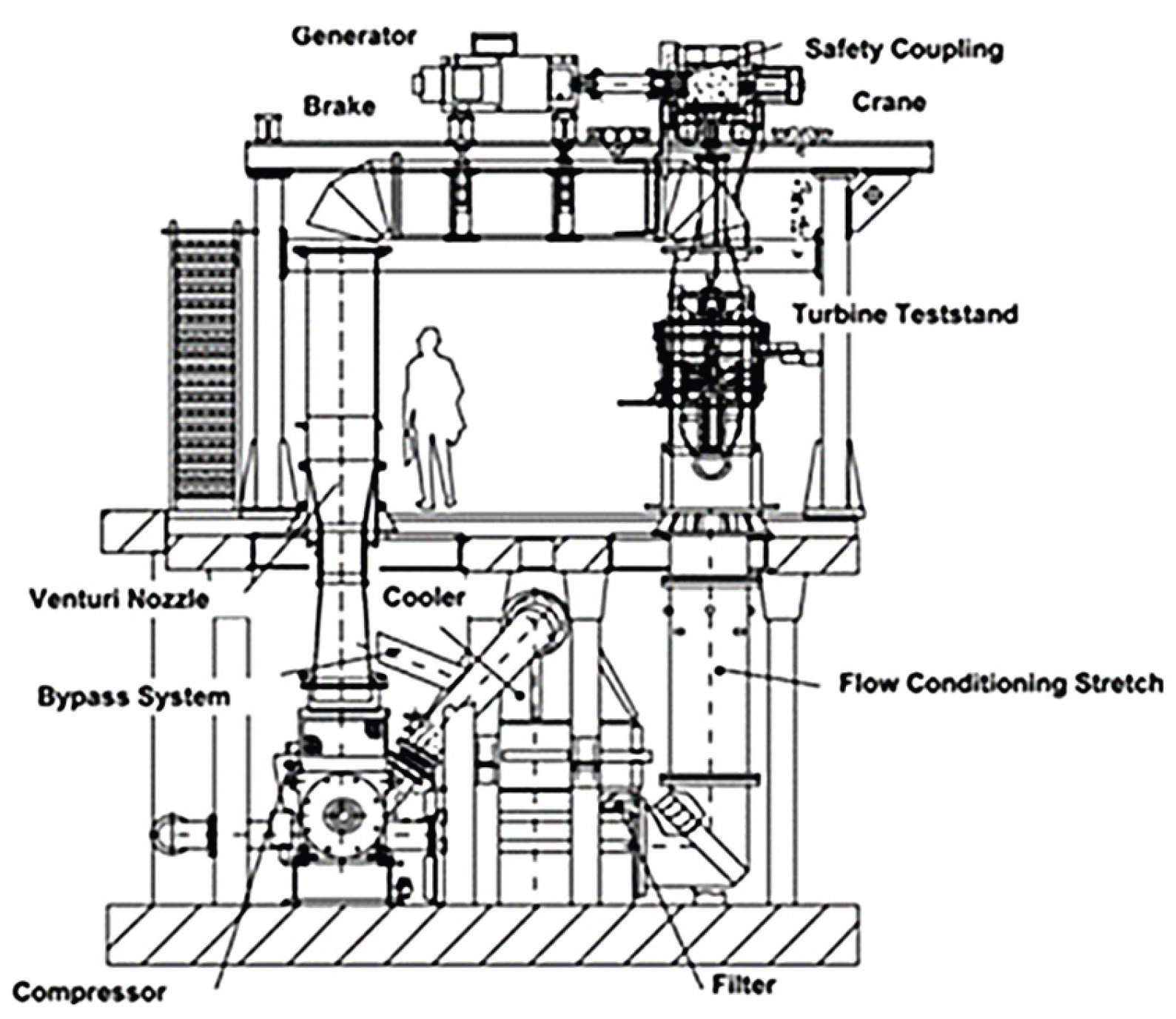
Figure 2.
Sketch of Axial Seal and data measurement’s locations.
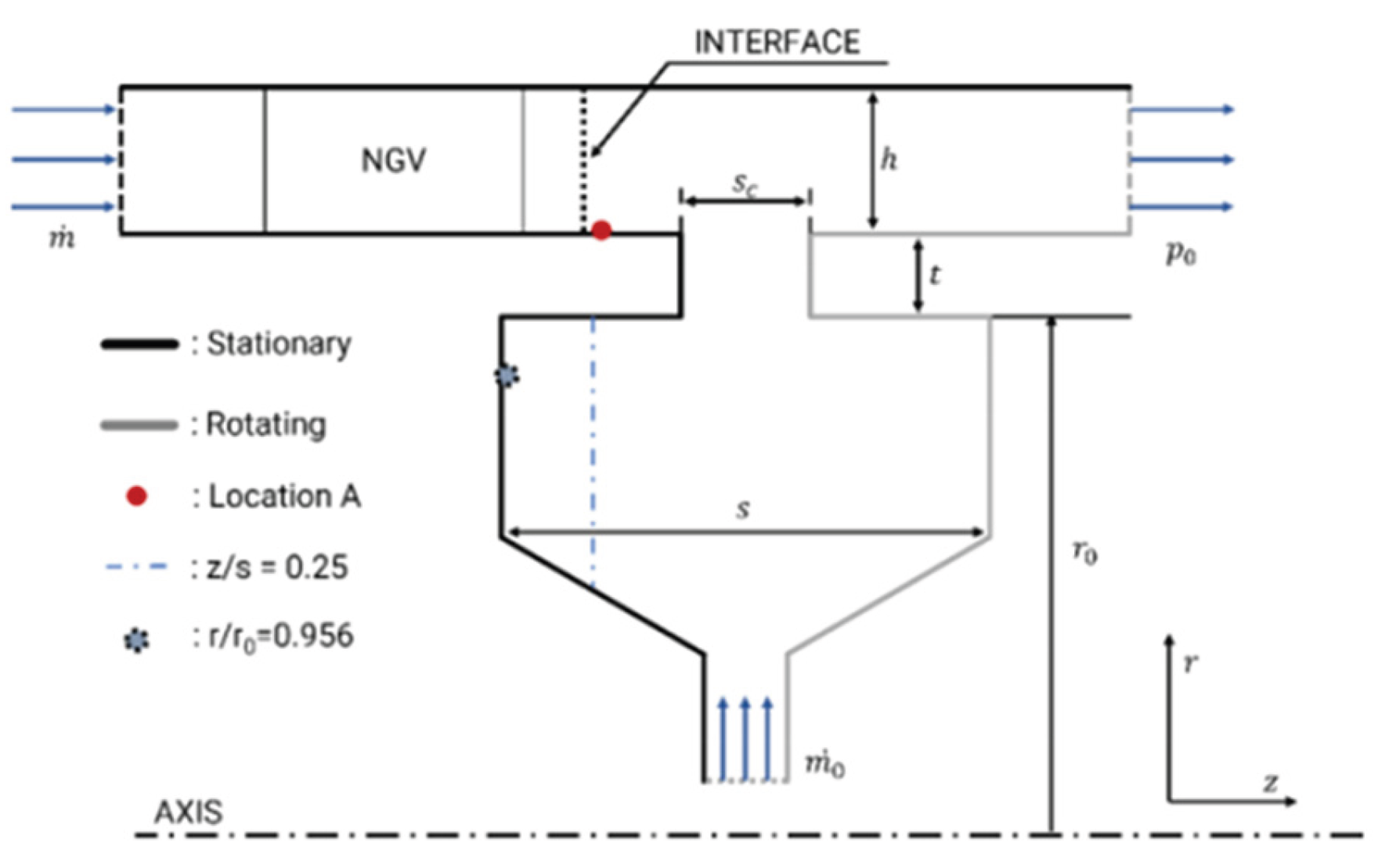
Figure 3.
Top view of measured plane for 1.5 stage LIS.
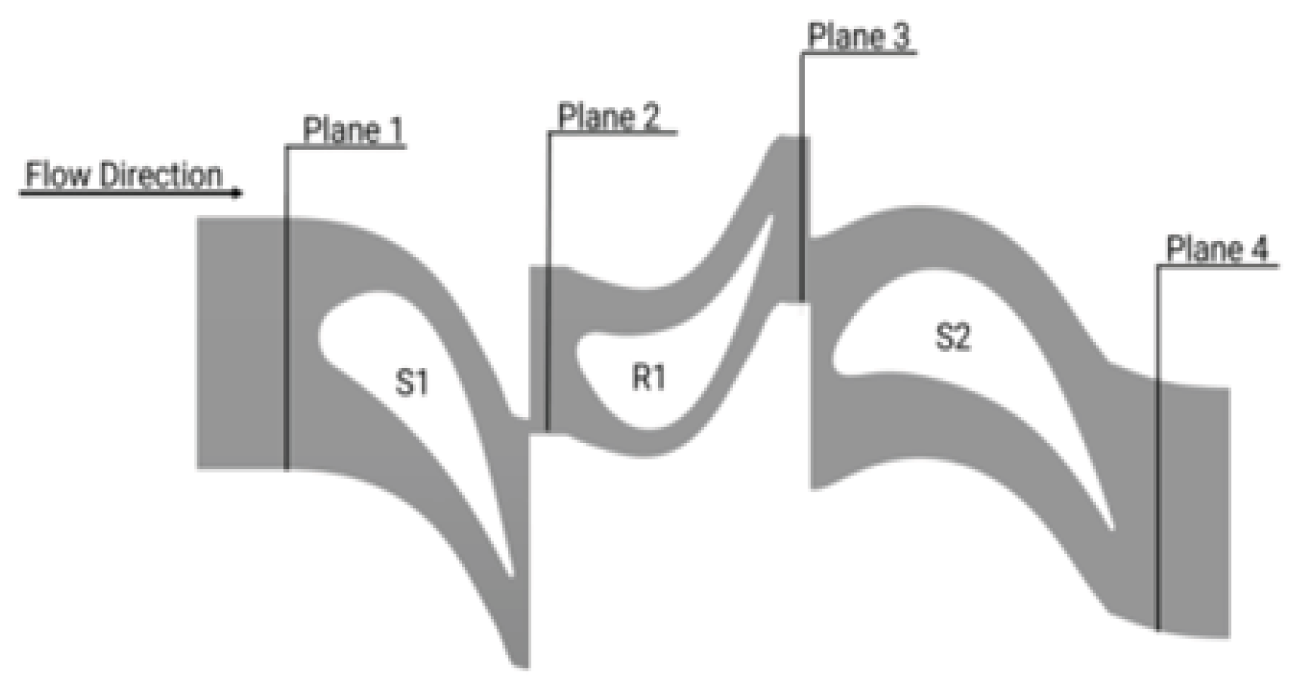
Figure 4.
1-stage LISA vane and blade mesh structure studies above.
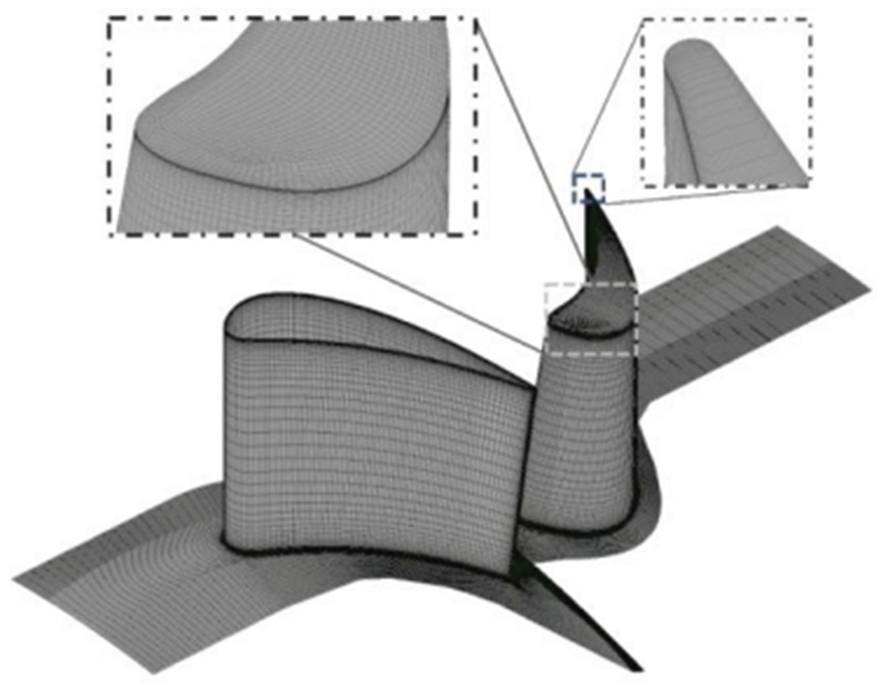
Figure 5.
1-stage LISA with axial seal geometry, including the meridional plane mesh of the rim seal.
Figure 5.
1-stage LISA with axial seal geometry, including the meridional plane mesh of the rim seal.
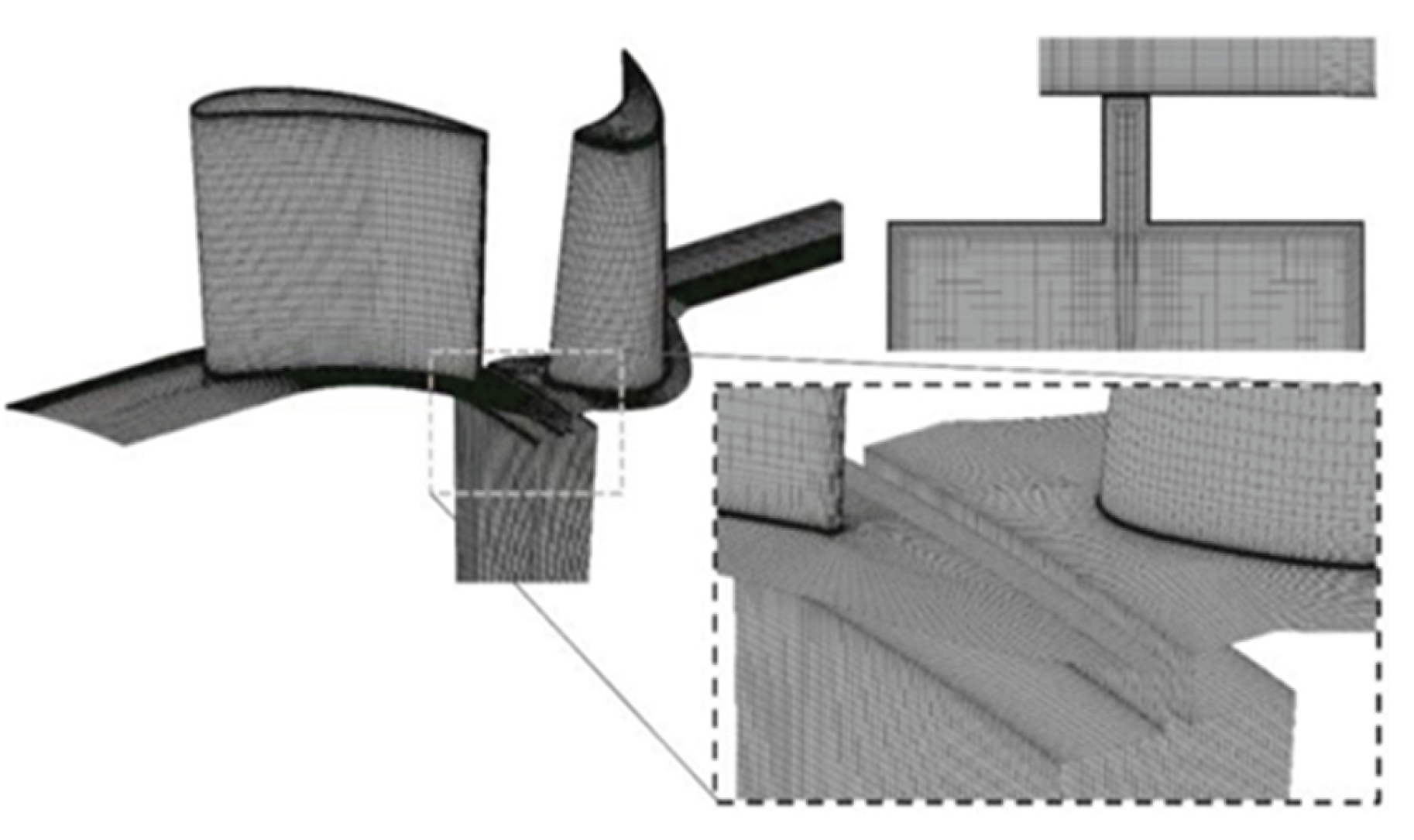
Figure 6.
Projection view of Stator vane single passage mesh by ICEM CFD.
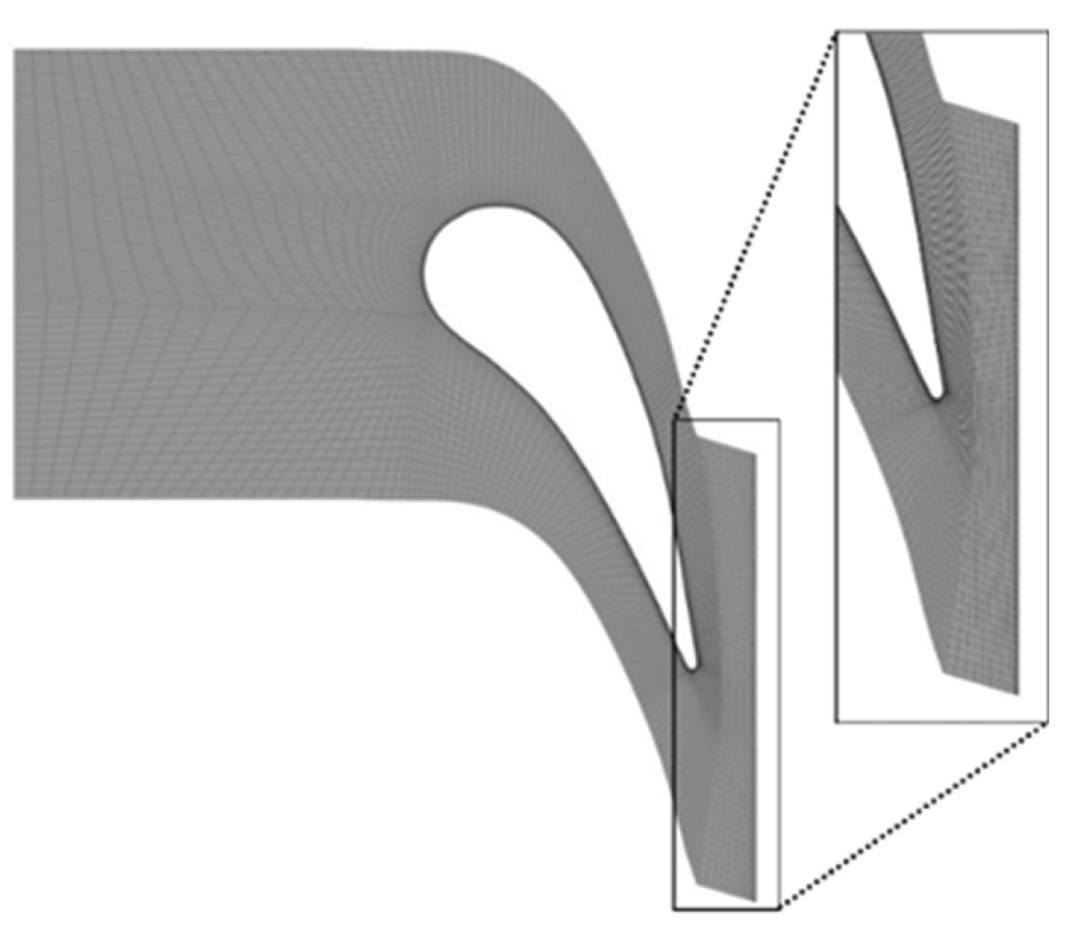
Figure 7.
Sketch of Radial Seal domain with wheel space submerged in the rotational part.
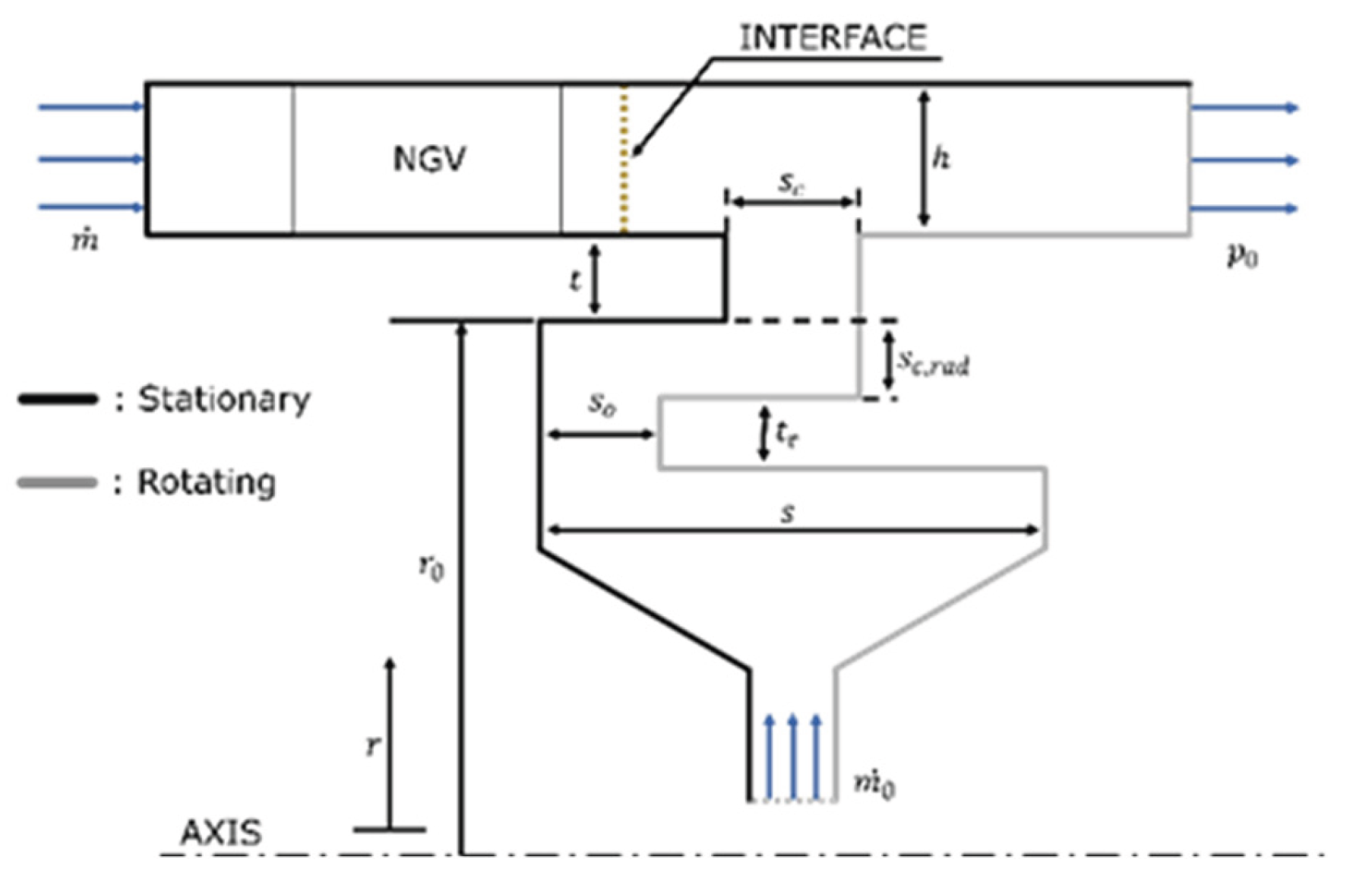
Figure 8.
Sketch of a “thin seal” approach with no interface involved.
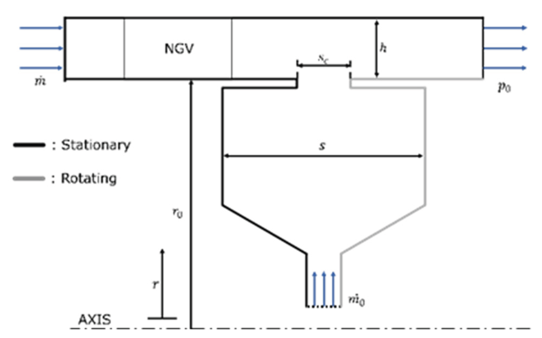
Figure 9.
Yawing angle at Plane 2 (S1) for three different mesh.
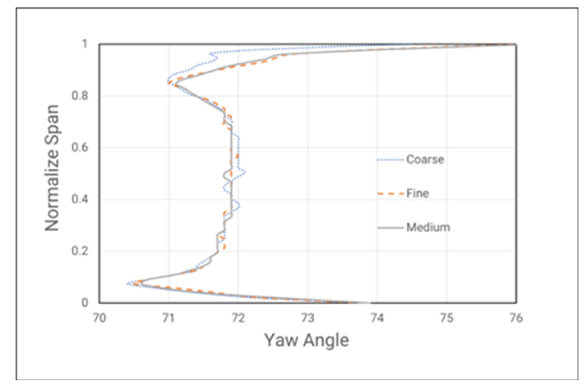
Figure 10.
Quantity validation of both 1.5/1 Stage LISA.
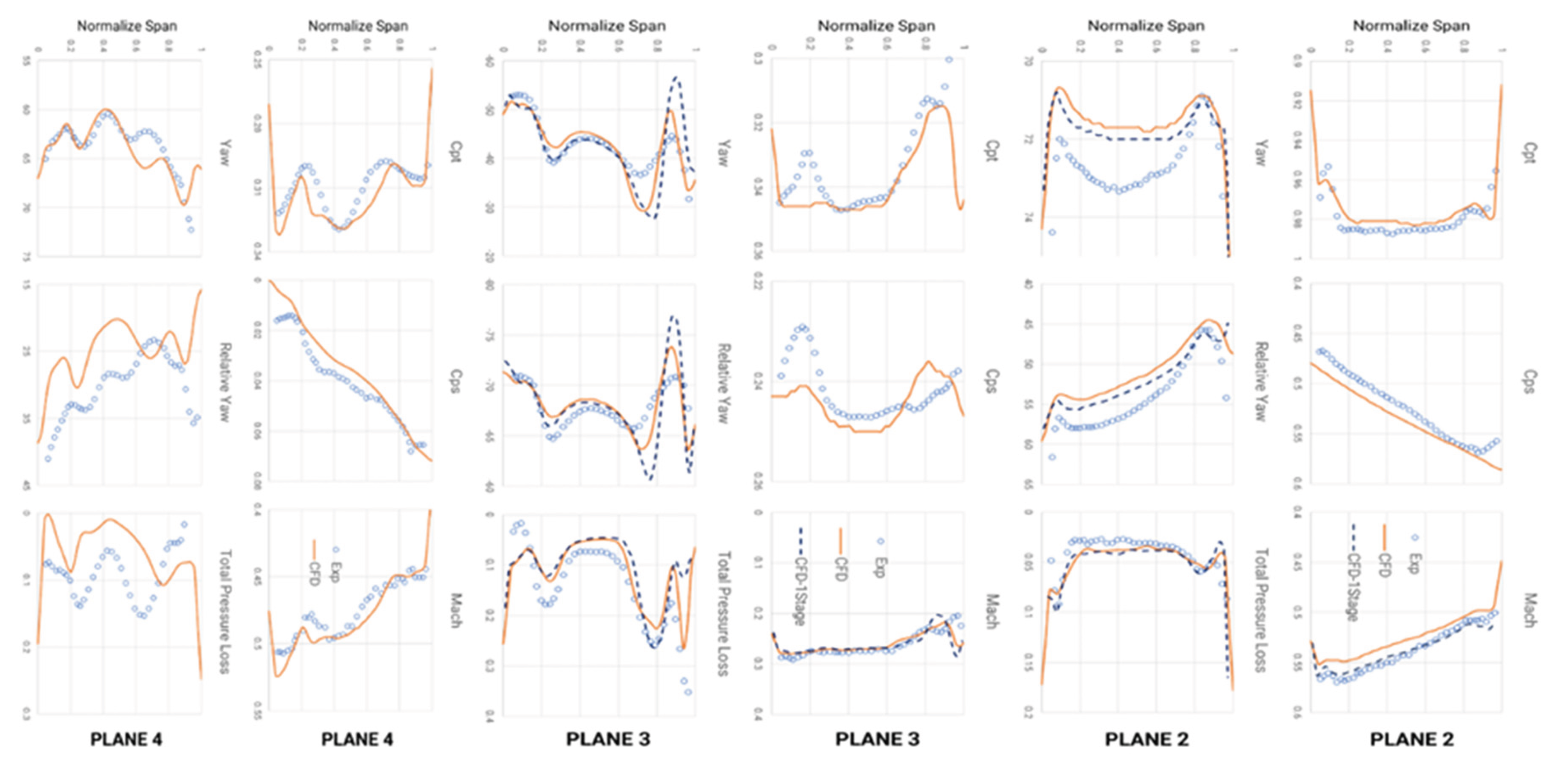
Figure 11.
Contour of y+ in Axial Rim Seal configuration at Φ0=0.03.
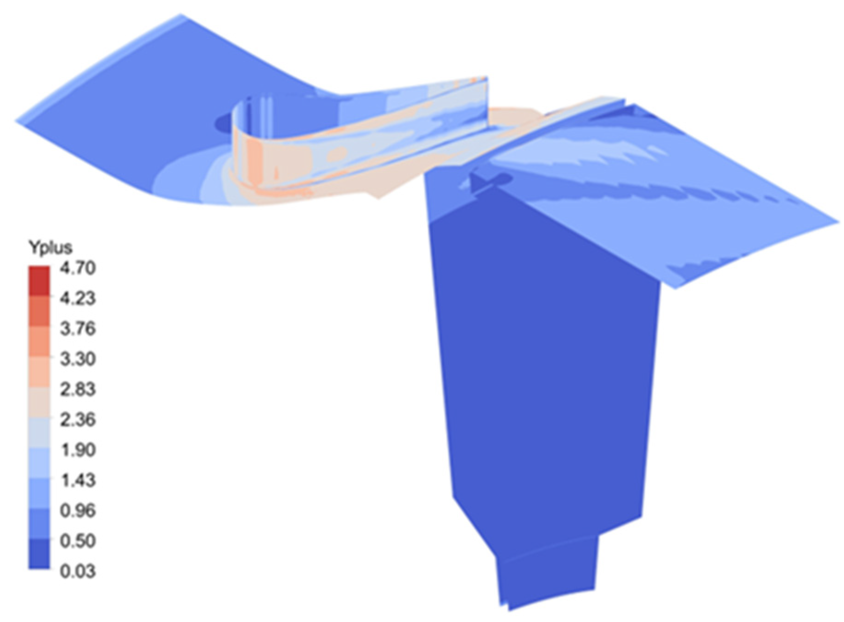
Figure 12.
Grid Convergence Index for Sealing Effectiveness and Peak-to-Trough Pressure at Location.
Figure 12.
Grid Convergence Index for Sealing Effectiveness and Peak-to-Trough Pressure at Location.
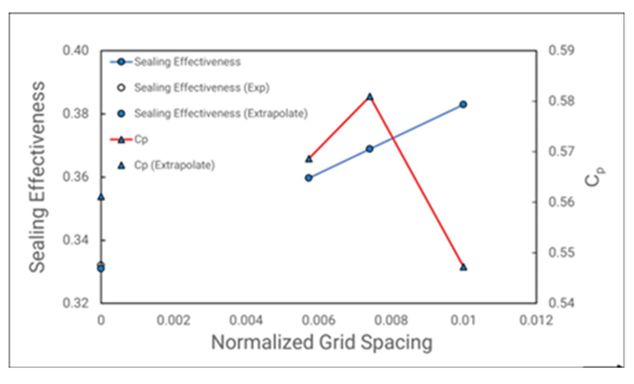
Figure 13.
Influence of Mesh on Pressure Distribution at Φ0 = 0.03.
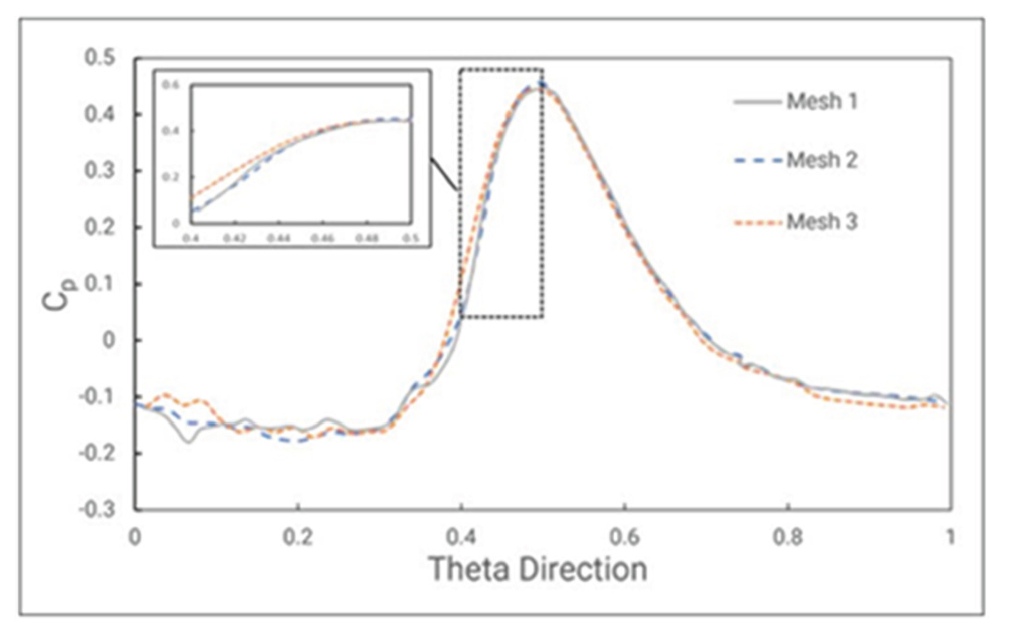
Figure 14.
Swirl ratio measured at plane z/s =0.25 for three different mesh.
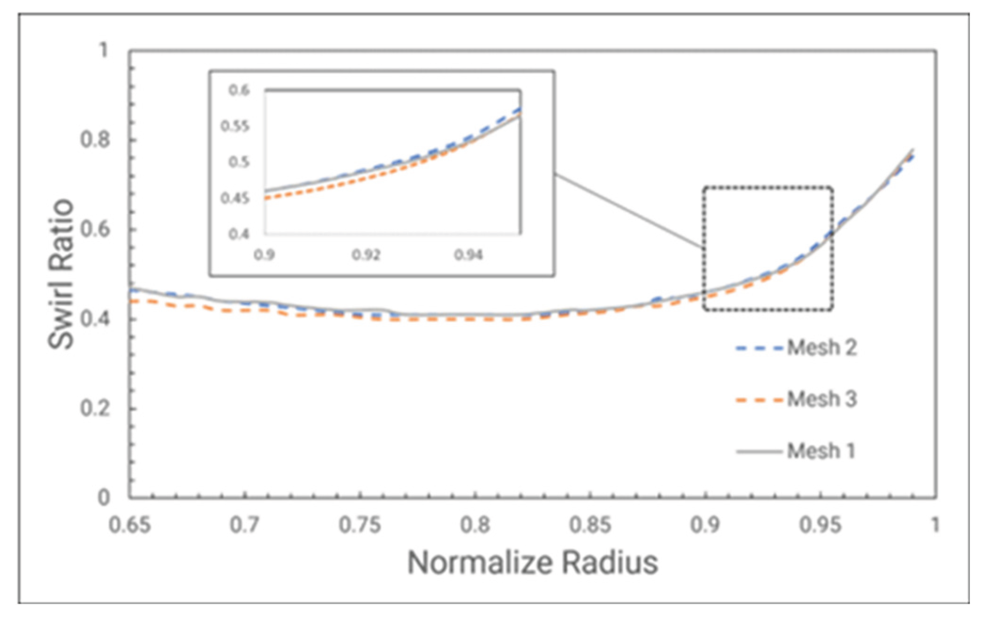
Figure 15.
Grid Convergence Index for Thin Seal configuration at Φ0=0.043.
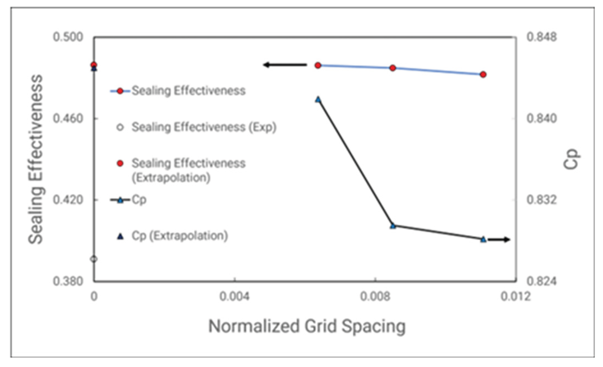
Figure 16.
Comparison of Pressure distribution along one stator vane.
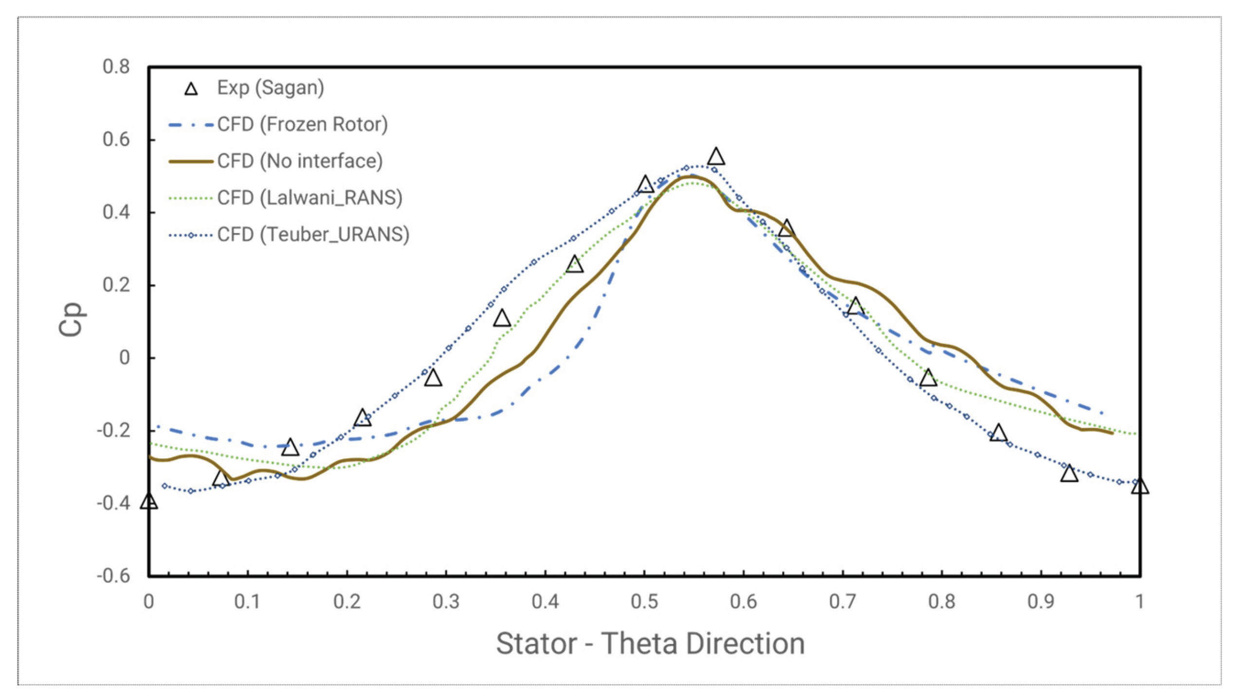
Figure 17.
Comparison of the square root of peak to trough pressure with the Operating condition.
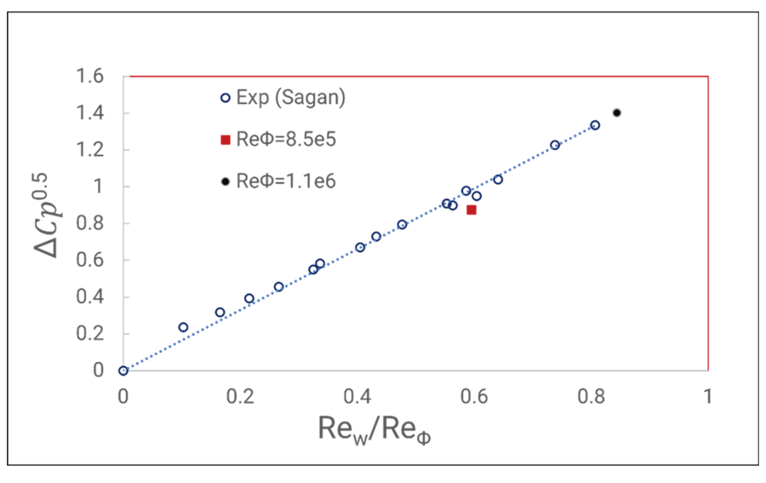
Figure 18.
Comparison of the velocity flow field inside the rim seal at r/r0 = 0.8.
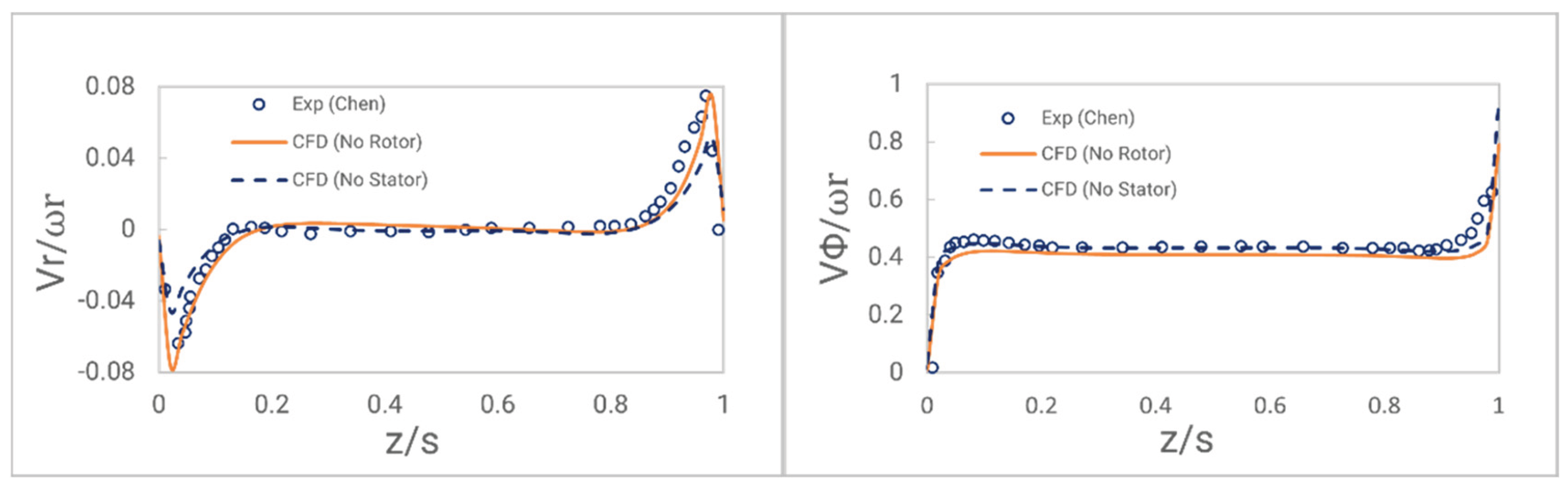
Figure 19.
Comparison of Swirling flow at plane z/s = 0.25 for Rim seal configuration #1.
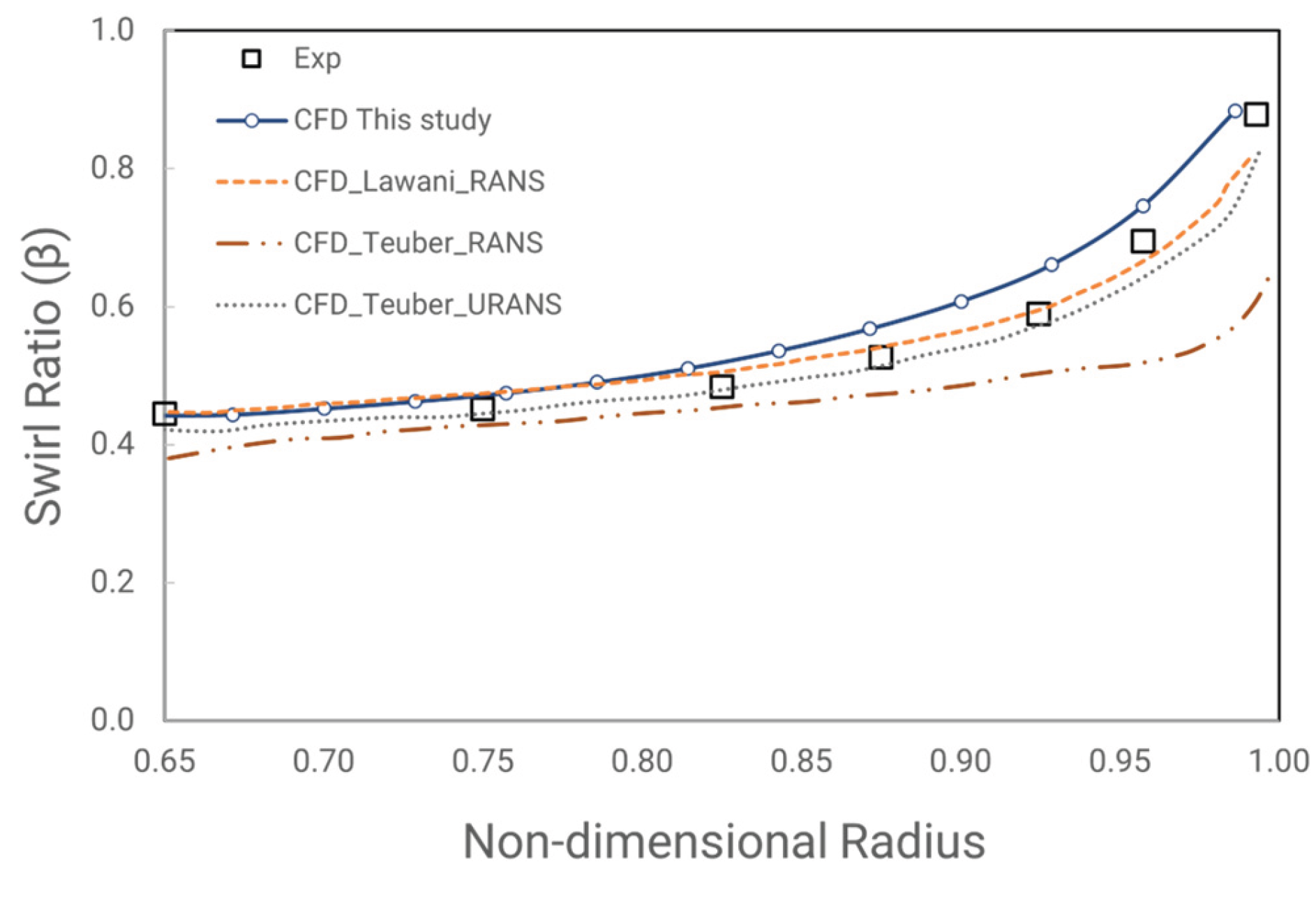
Figure 20.
Comparison of Swirling flow at plane z/s = -0.75 for Rim seal configuration #2.
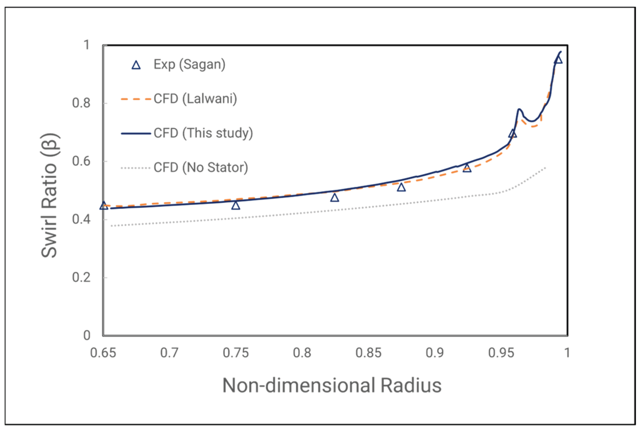
Figure 21.
Sealing Effectiveness for entirely stationary frame wheel-space.
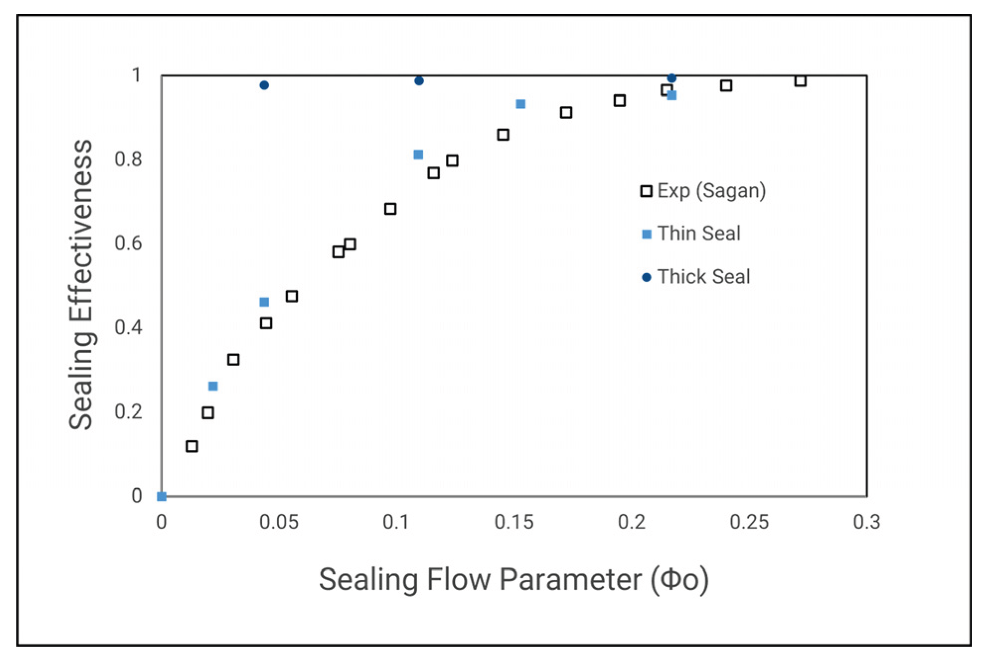
Figure 22.
Contour of Sealing effectiveness in Radial-Theta direction to the flow view for three types of domains for Gen#4 configuration at Φ0 =0.045.
Figure 22.
Contour of Sealing effectiveness in Radial-Theta direction to the flow view for three types of domains for Gen#4 configuration at Φ0 =0.045.
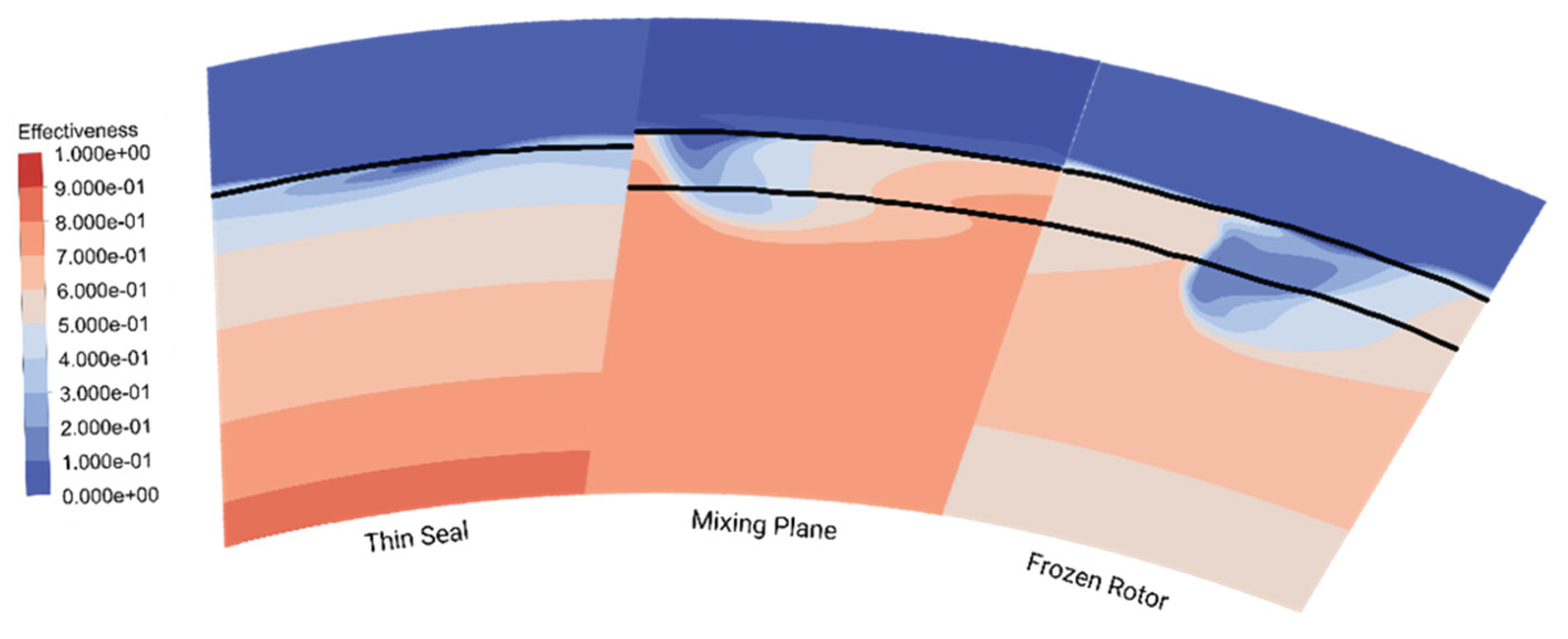
Figure 23.
Theoretical Orifice Model for Thin Seal Approach.
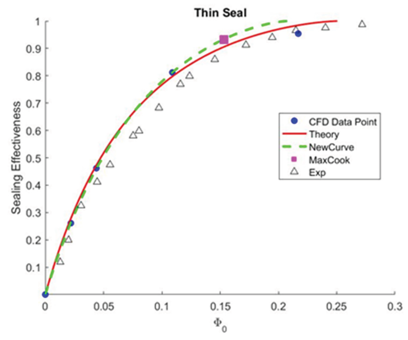
Figure 24.
Sealing effectiveness of Gen#4 rim seal configuration with MRF method.
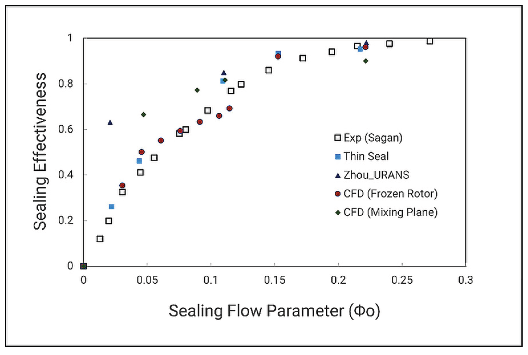
Figure 25.
Sealing effectiveness of Gen#2 rim seal configuration with MRF method.
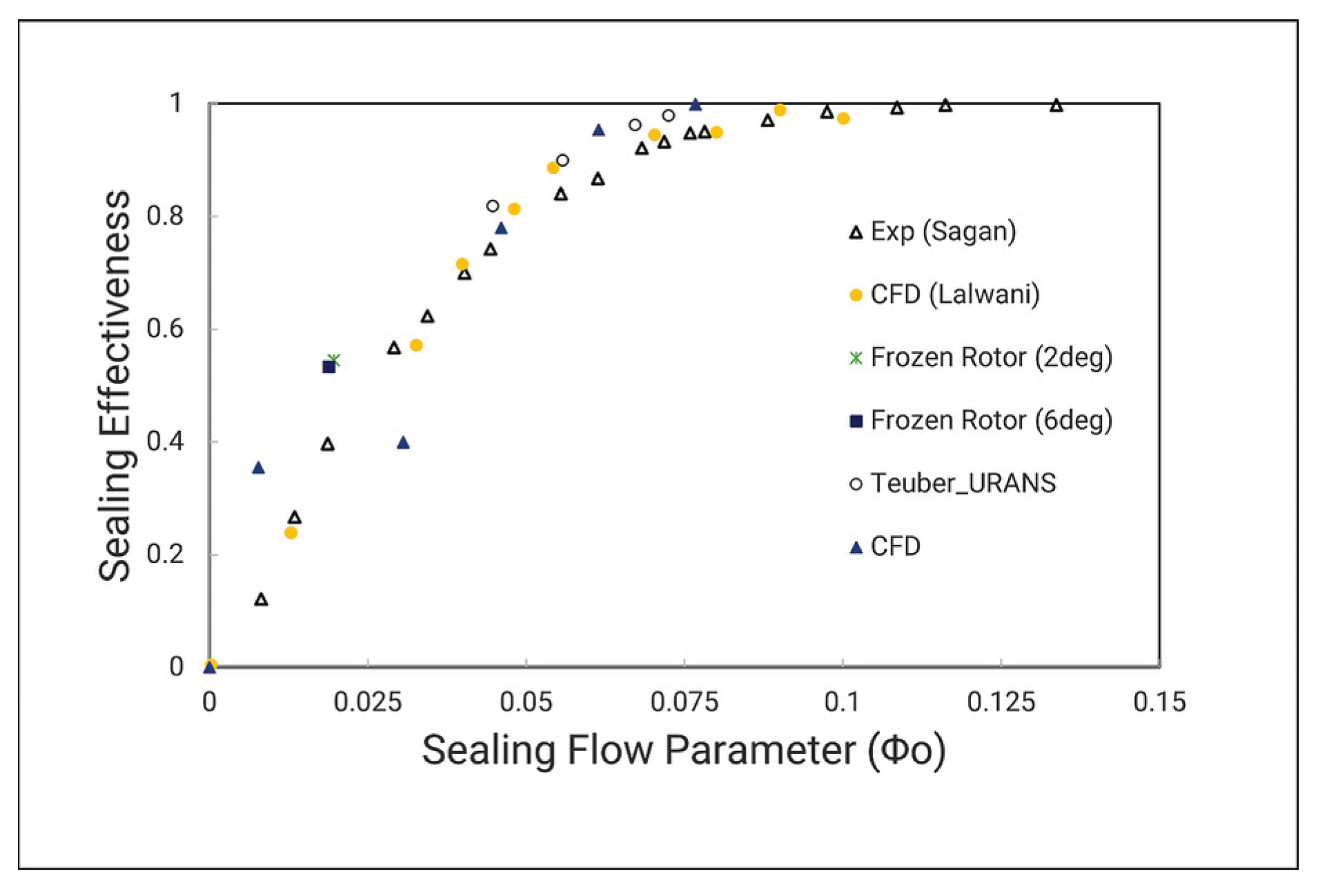
Figure 26.
Theoretical Orifice Model for Radial Rim Seal Configuration.
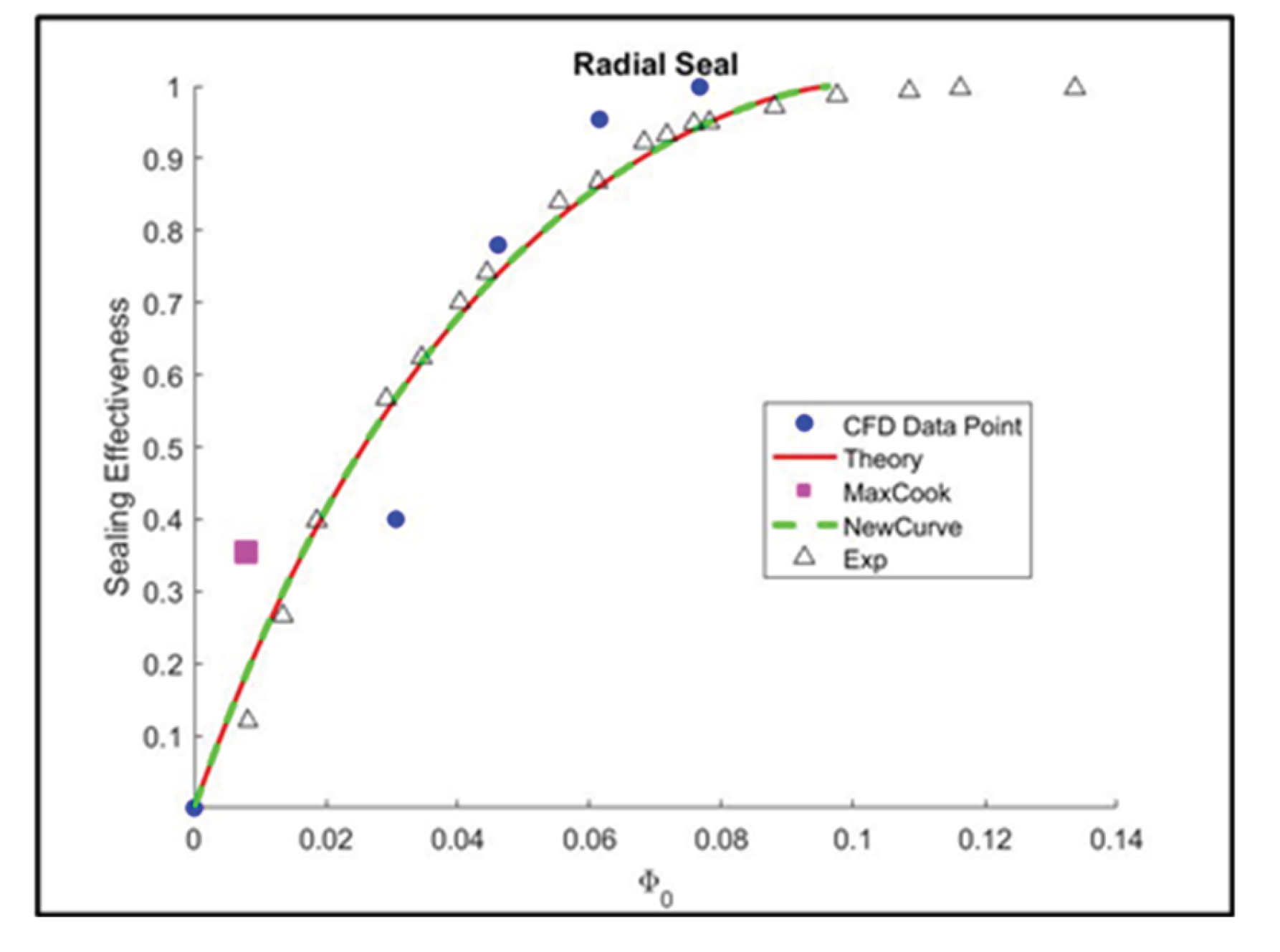
Figure 27.
Sealing effectiveness of Gen#1 rim seal configuration with MRF method.
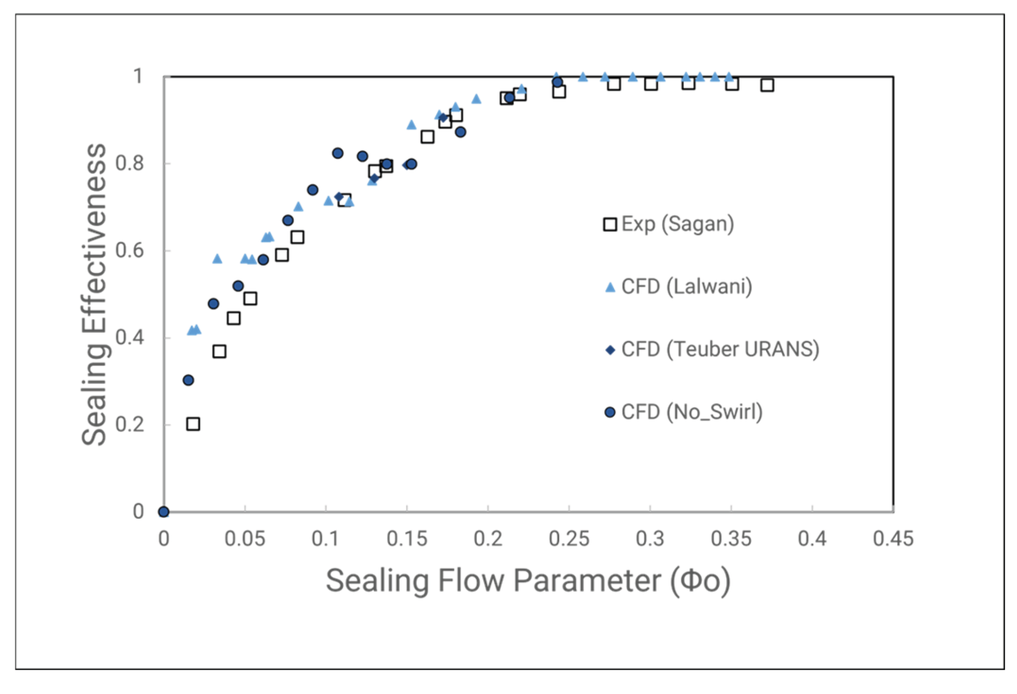
Figure 29.
Sealing Effectiveness Function for Axial Seal with removing lower sealing flow data.
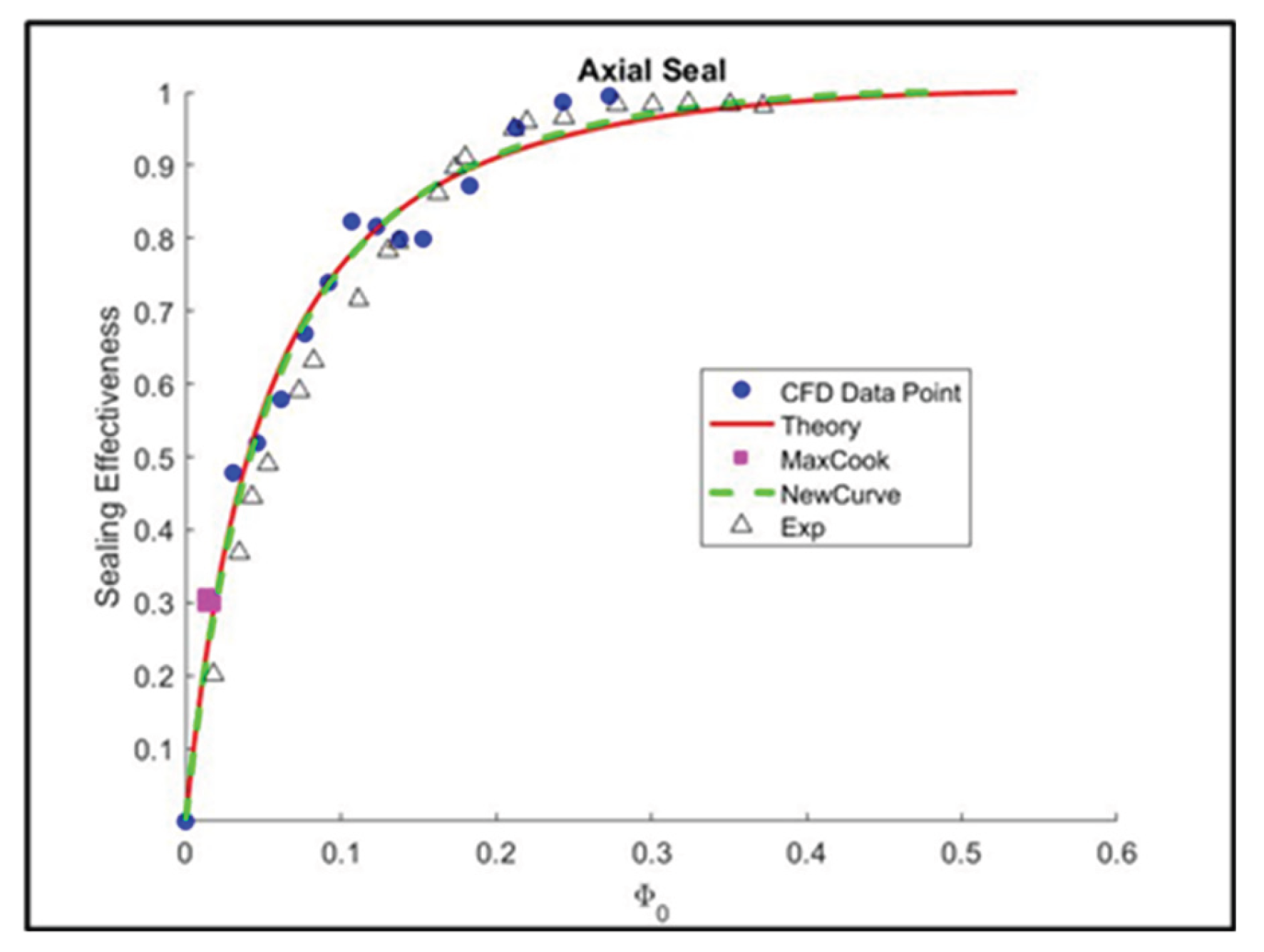
Figure 30.
Pressure distribution at Location A for two different interface models.
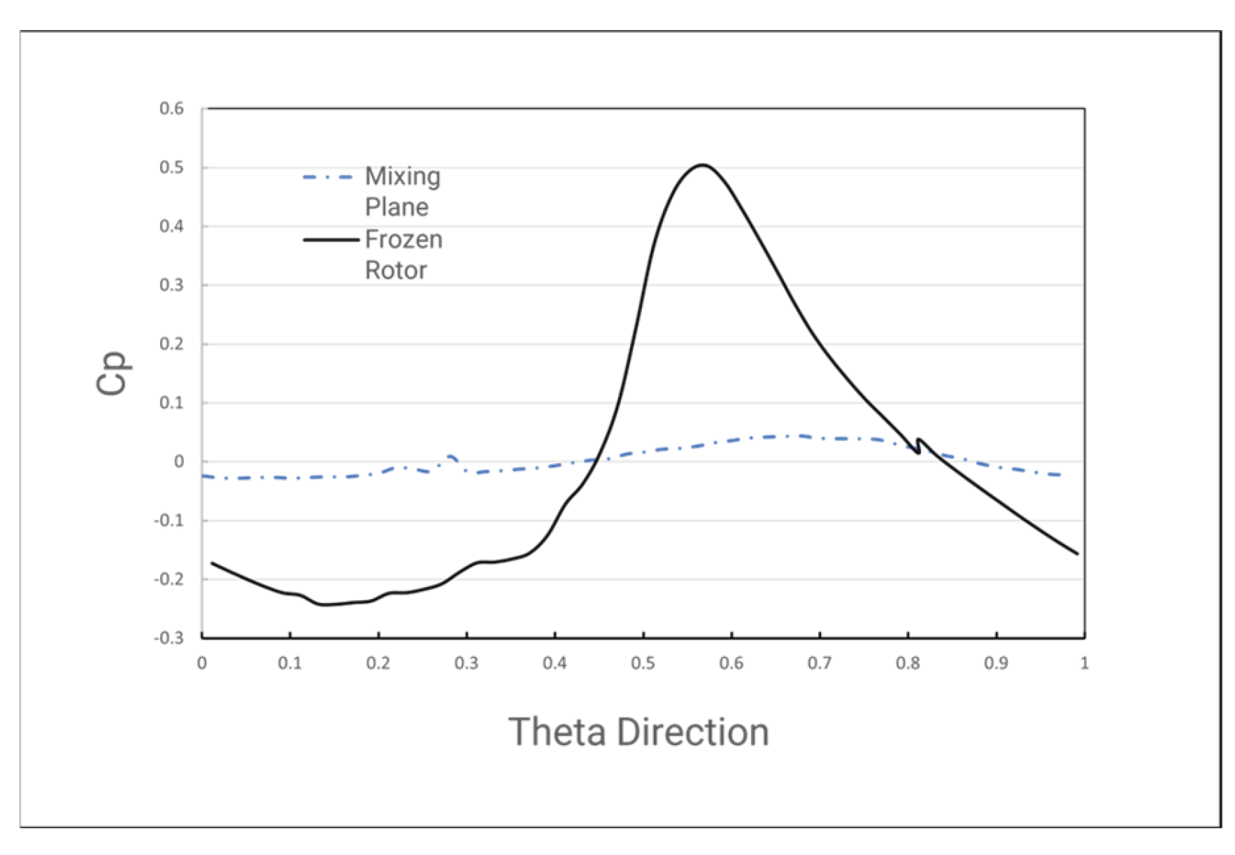
Figure 31.
Sealing Effectiveness of Axial Rim Seal with Pre-Swirl and Swirl cooling flow.
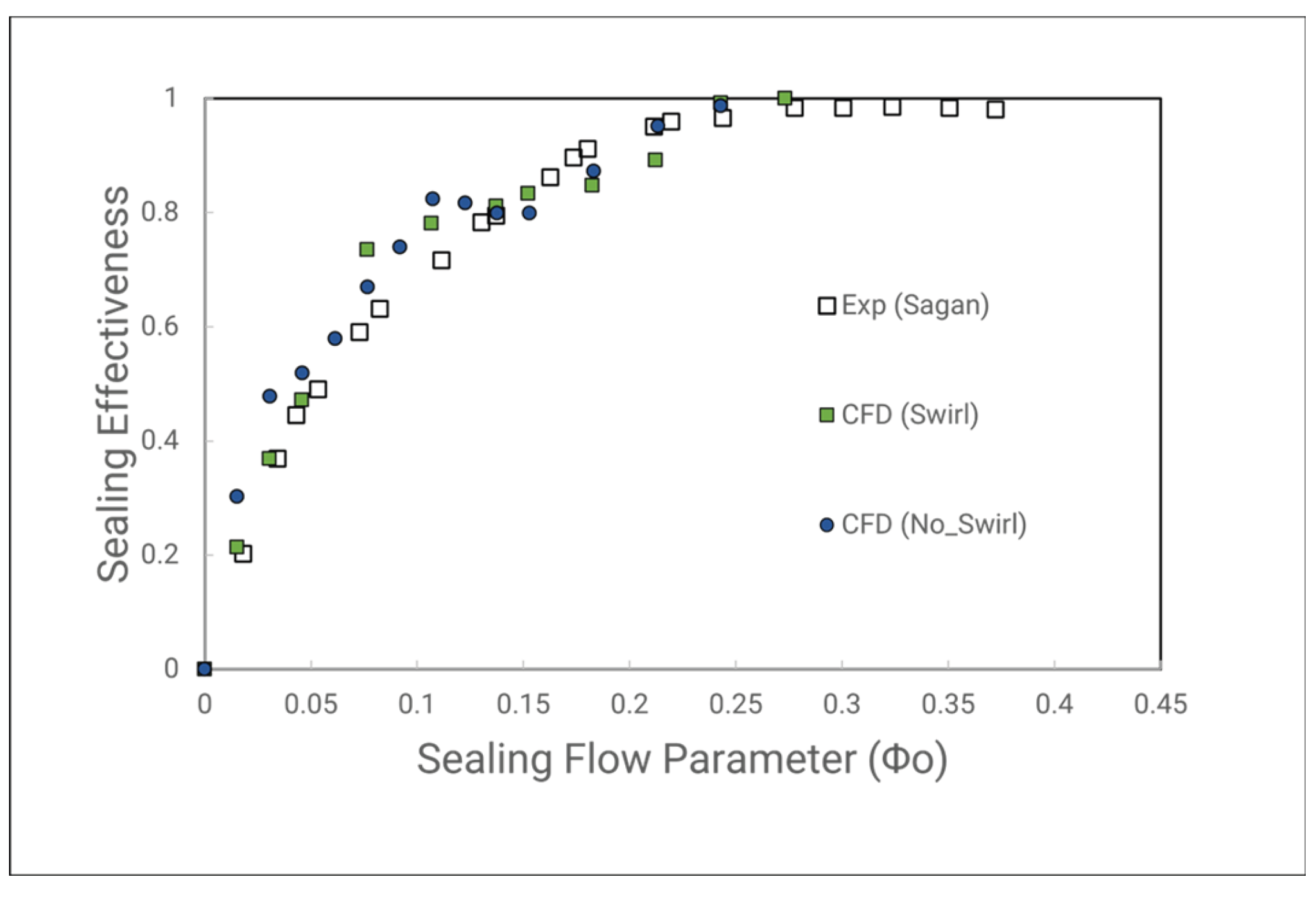
Figure 32.
Sealing Effectiveness Function for Axial Seal with Swirling Flow.
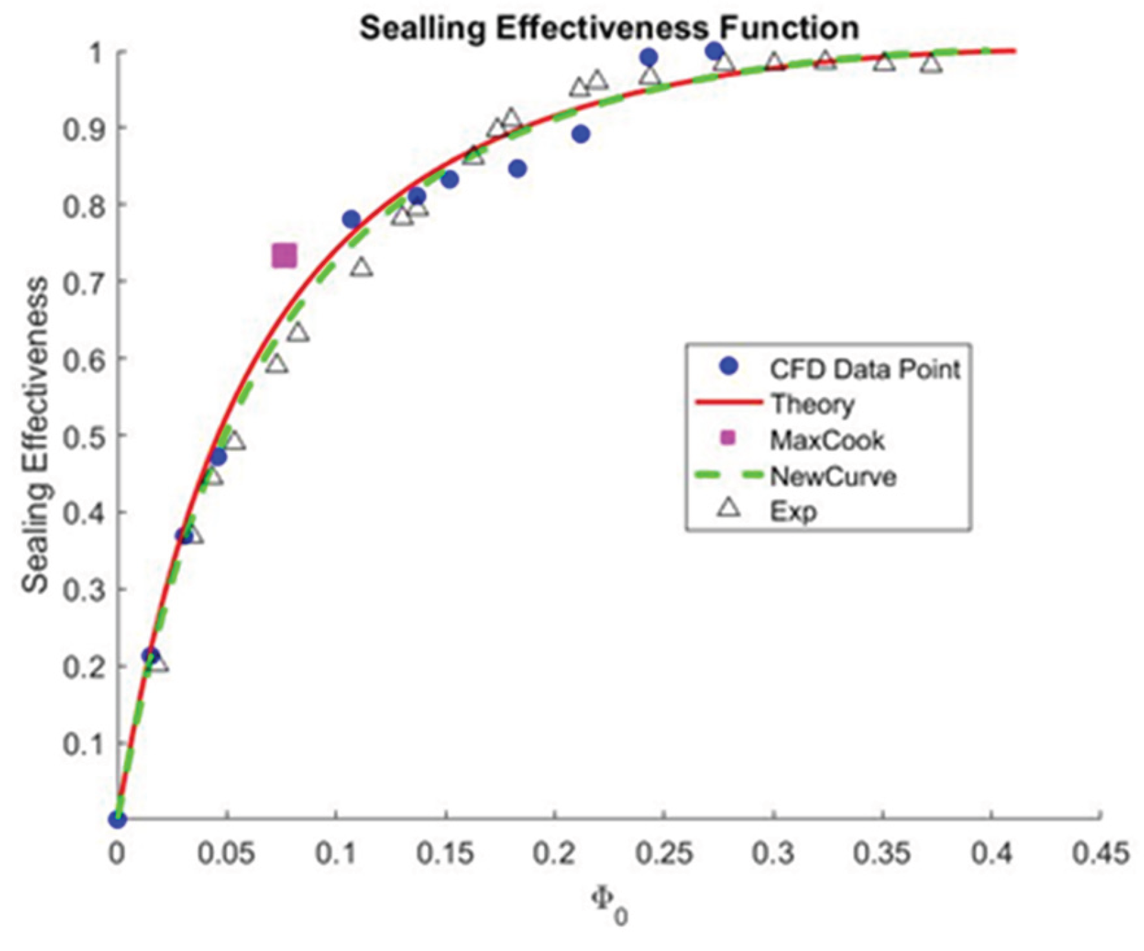
Figure 33.
Moment coefficient on the Rotor wall Swirl and No Swirl for Axial Seal.
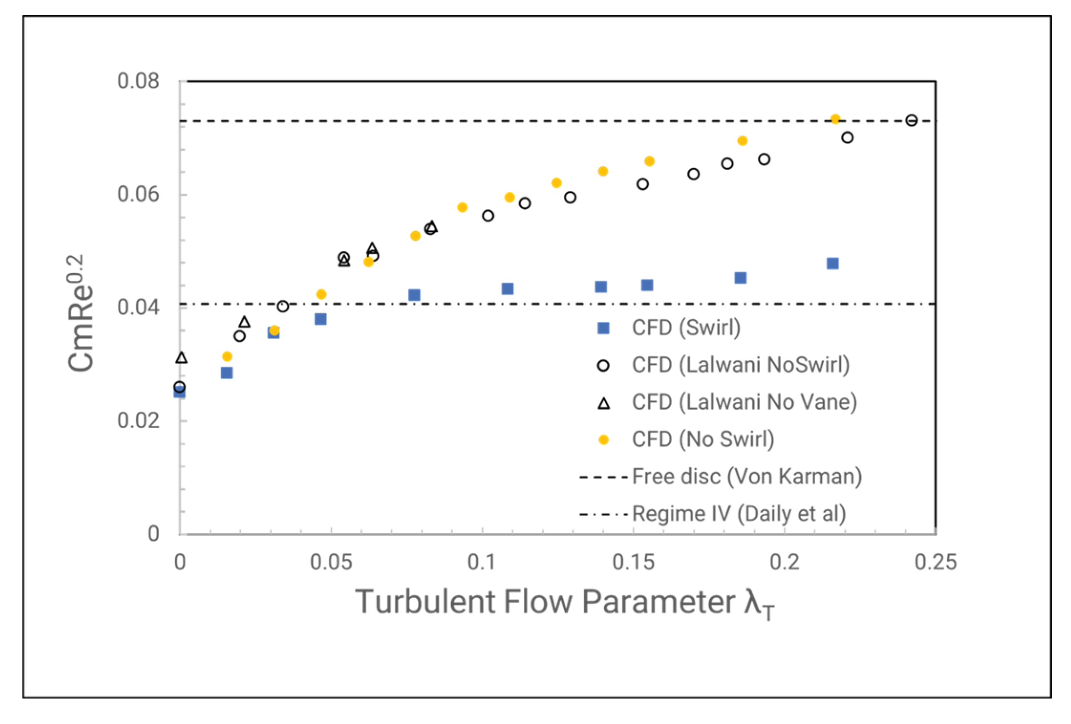
Figure 34.
Moment coefficient on the Rotor wall Swirl and No Swirl for Radial Seal.
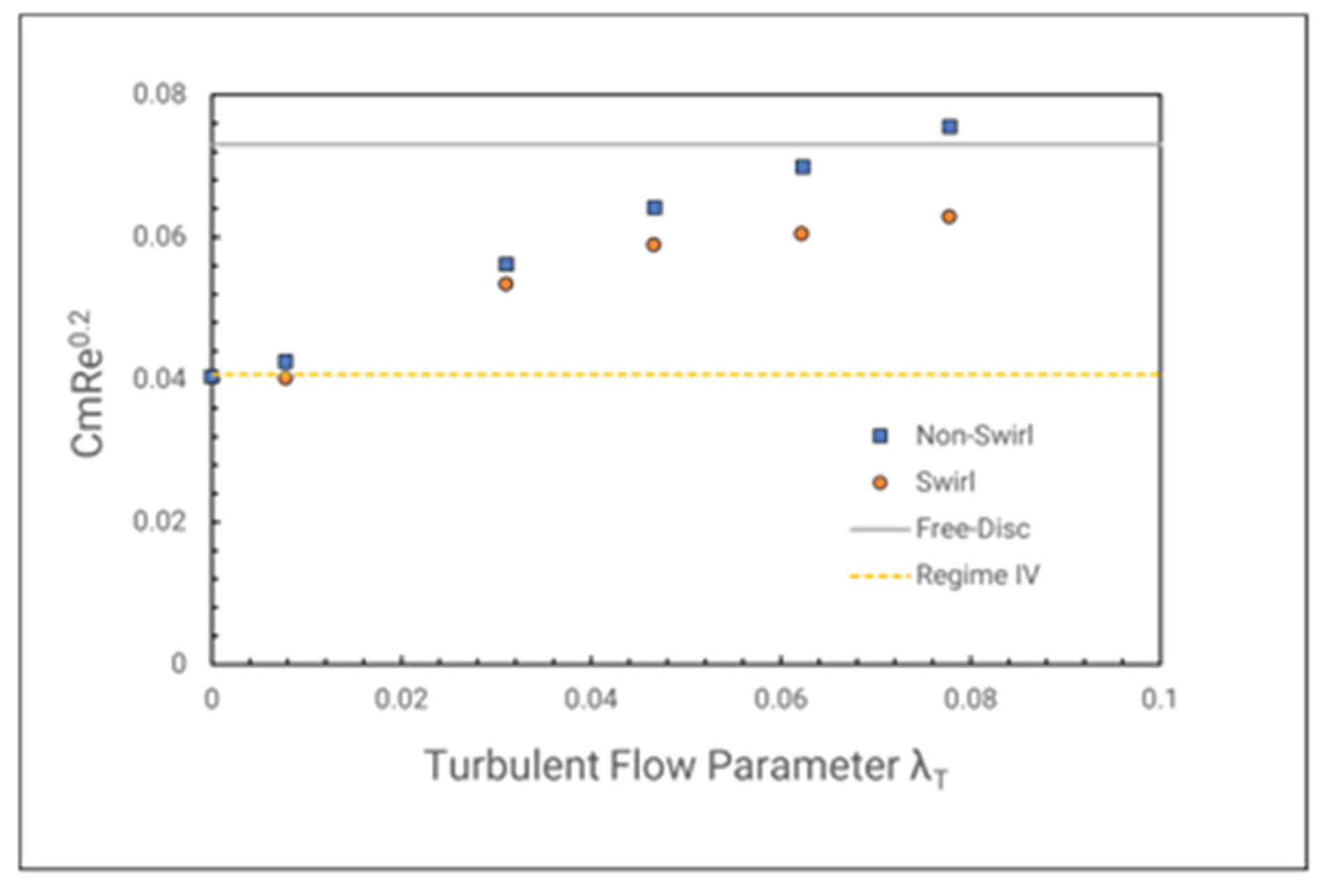
Figure 35.
Wall Shear pressure distribution on the overlap region in Radial Rim Seal.
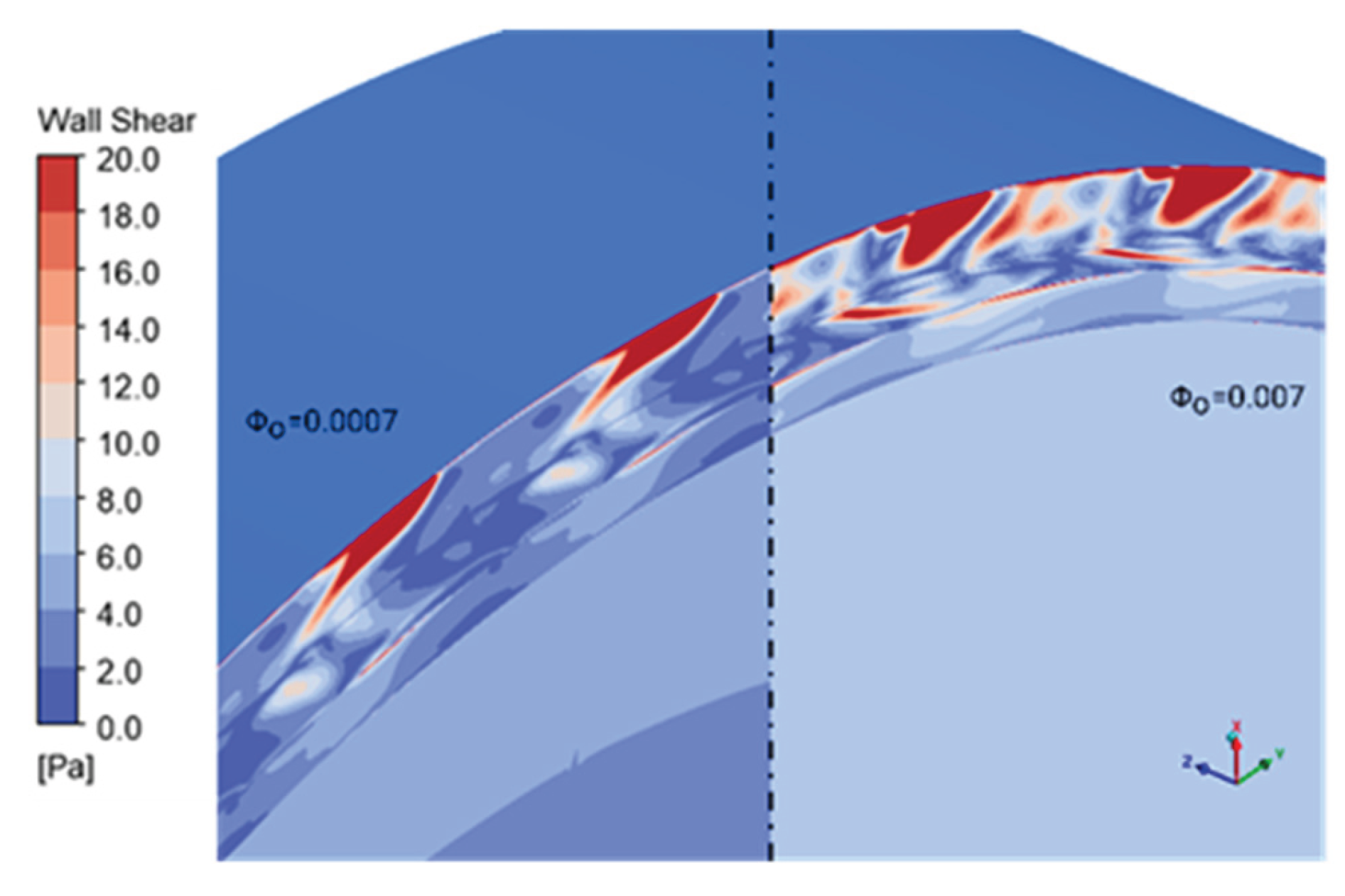
Figure 36.
Contour of Sealing effectiveness and Normalize (Gauge) Pressure at Middle the rim seal gap (Gen# 4), Looking from Axial and Radial Position at 0.71 blade passing period.
Figure 36.
Contour of Sealing effectiveness and Normalize (Gauge) Pressure at Middle the rim seal gap (Gen# 4), Looking from Axial and Radial Position at 0.71 blade passing period.
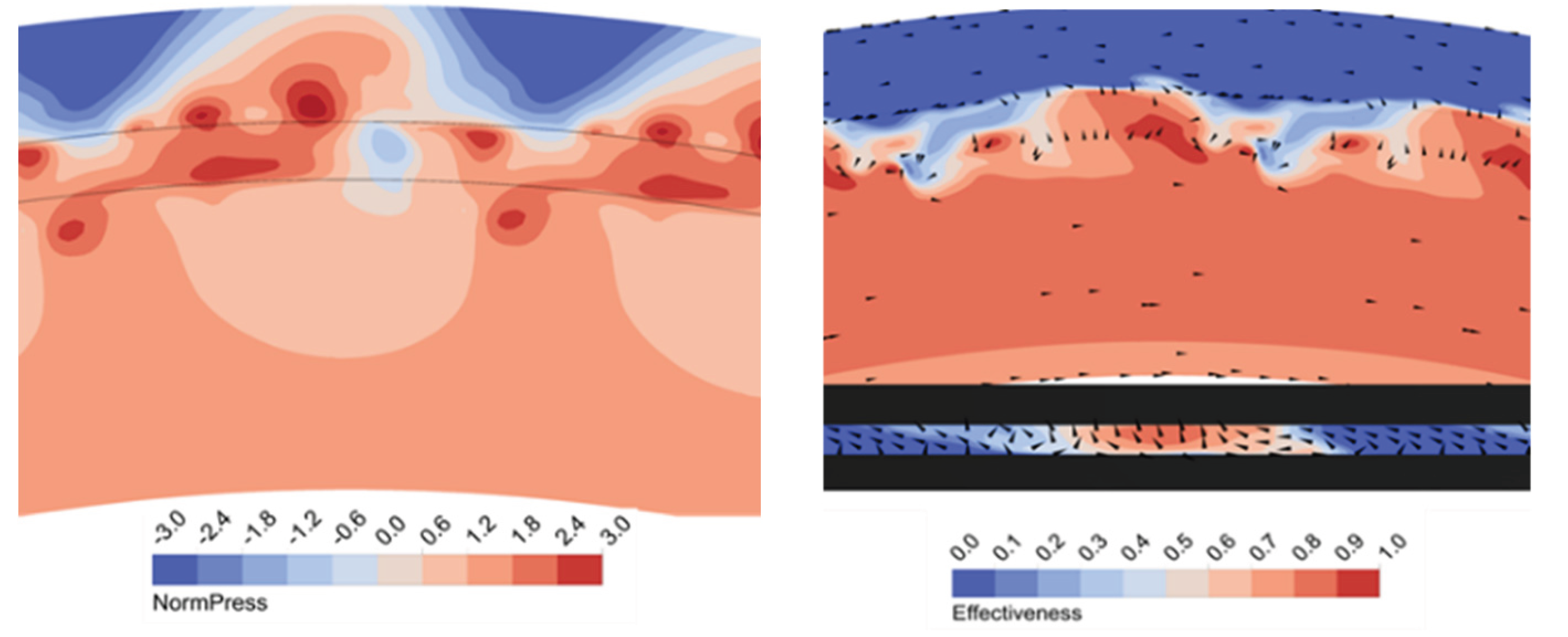
Figure 37.
Pressure at Monitor point (Right) against frequency domain.
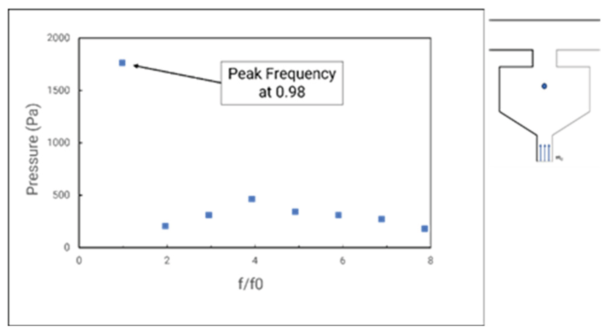
Figure 38.
Sealing Effectiveness at Monitor point (Right) against Frequency Domain.
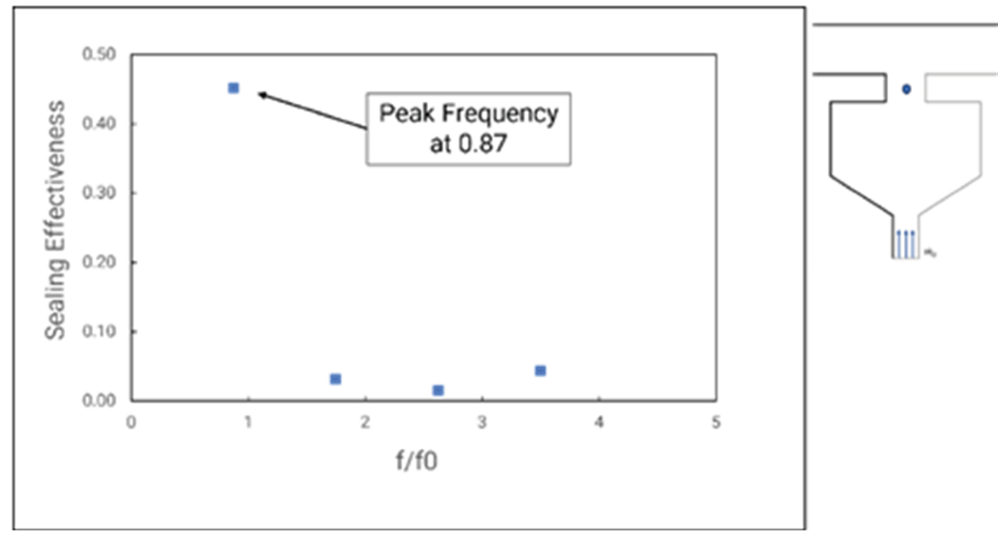
Figure 39.
Frozen Rotor blade Angle.
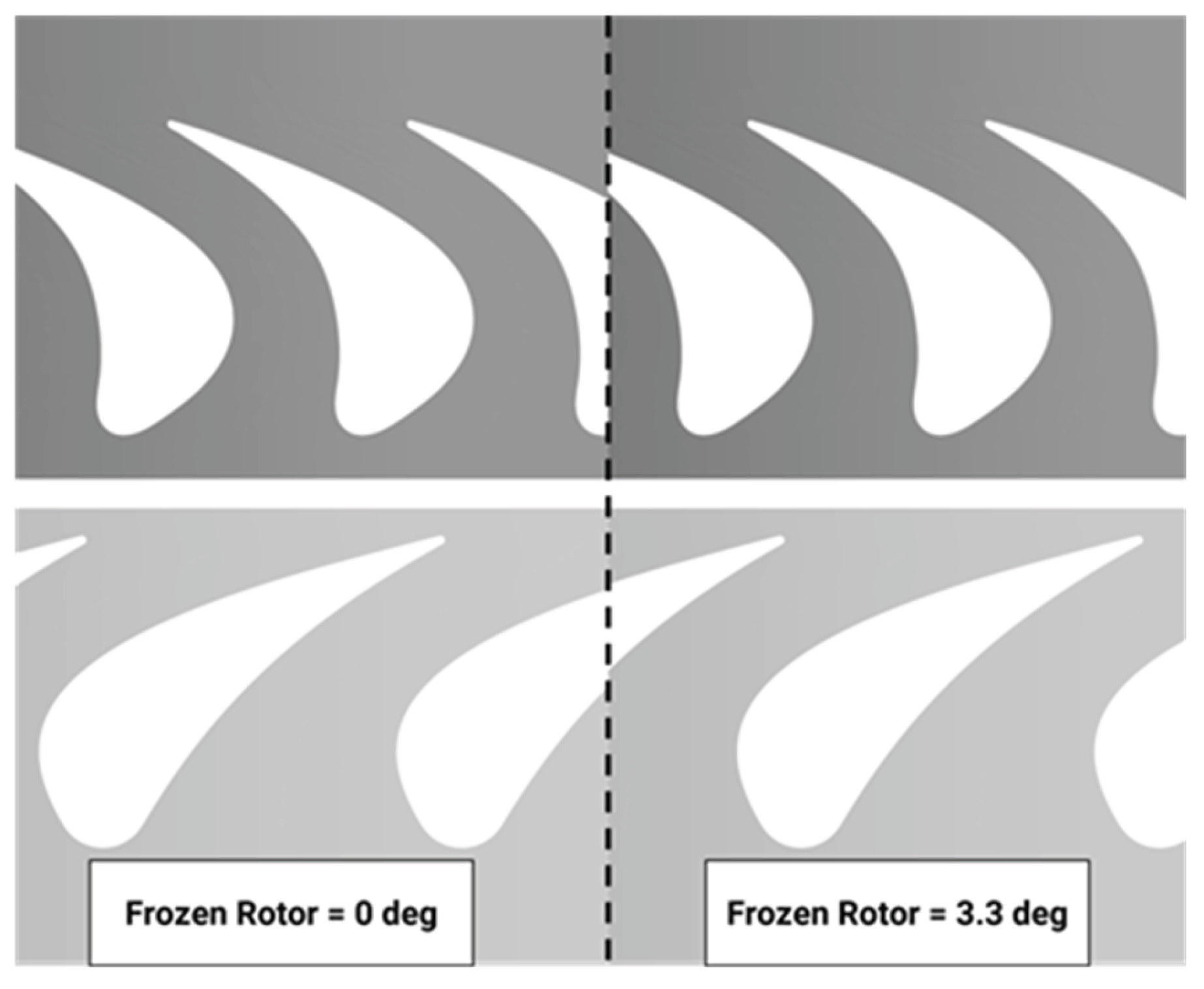
Figure 40.
Streamline ISO and Projection view in the rim seal region.
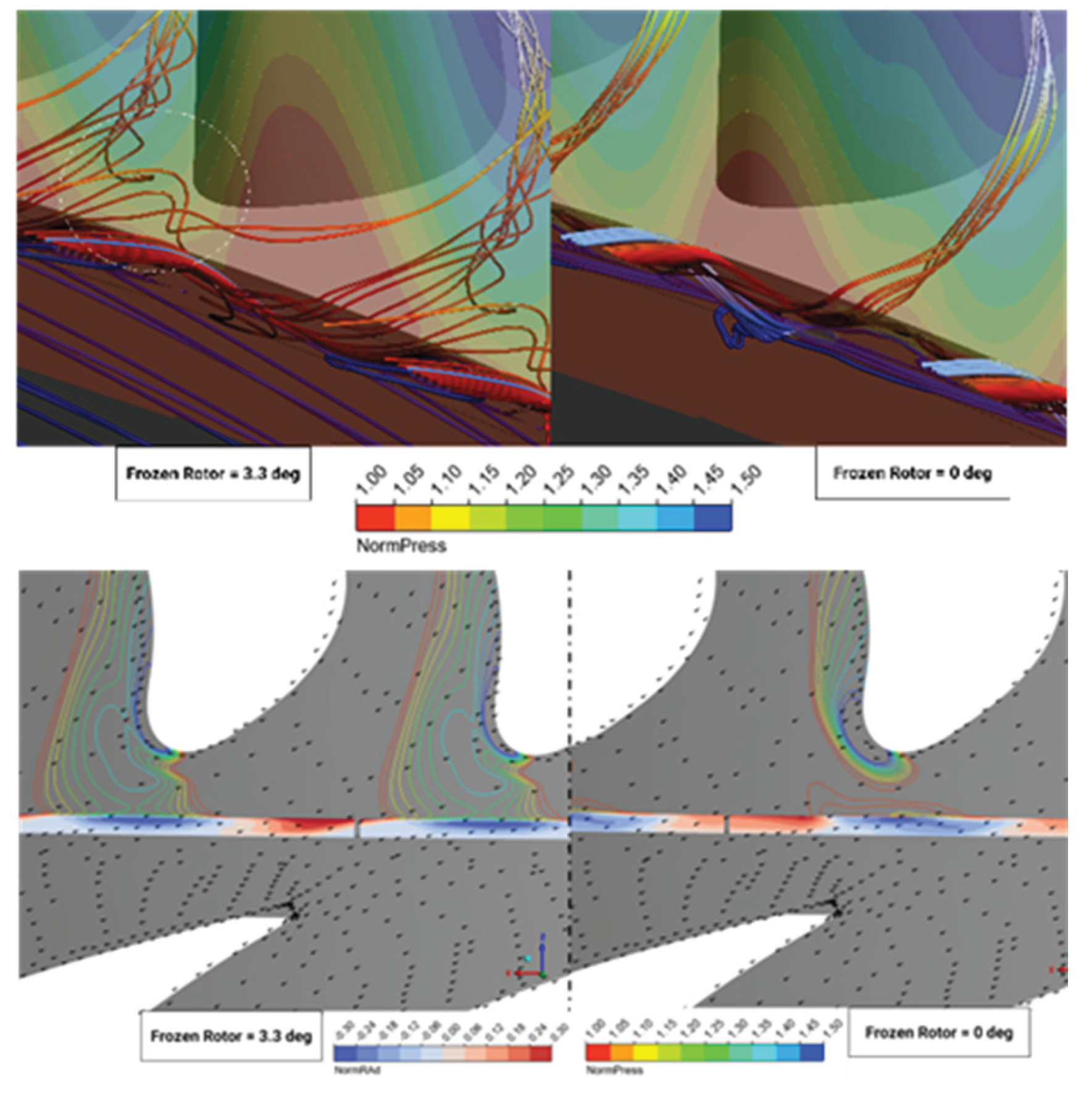
Figure 41.
Total Pressure losses comparison between baseline and rim seal turbine.

Figure 42.
Vector-contour and Streamline near the rim seal gap at flow rate =0.05%.
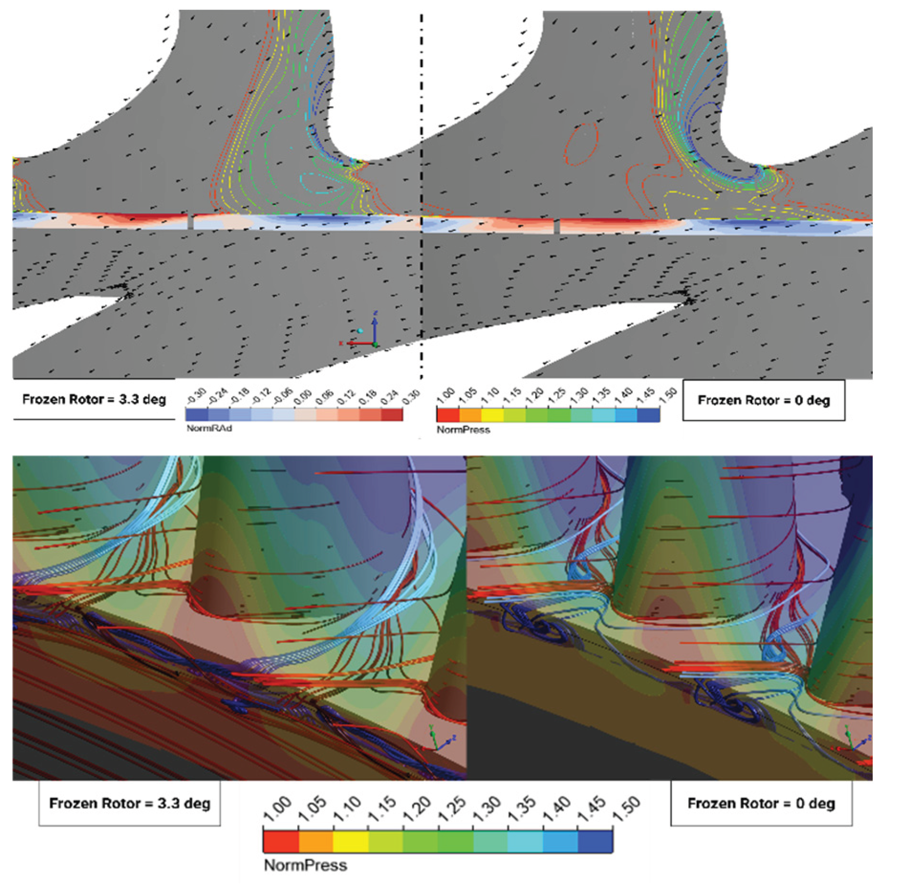
Table 2.
Results of GCI investigation for Axial Rim Seal at Φ0 = 0.03.
| Variable | Symbol | Experimental | 1.5 Stage | Relative Error (%) | 1 Stage | Relative Error (%) |
| Total to static pressure | Π1.5 | 1.6 | 1.601 | 0.062 | ||
| Total to total pressure | Π1 | 1.353 | 1.346 | 0.517 | 1.355 | 0.148 |
| Isentropic Efficiency | ηis | 0.91 | 0.904 | 0.604 | 0.913 | 0.330 |
| Load Coefficient | HT | 2.36 | 2.341 | 0.805 | 2.305 | 2.331 |
| Reaction Coefficient | R | 0.39 | 0.392 | 0.436 | 0.39 | 0.39 |
| Flow Coefficient | Φflow | 0.65 | 0.649 | 0.123 | 0.65 | 0.65 |
| Mass Flow Rate | 11.7 | 11.91 | 1.795 | 11.87 | 1.453 | |
| Total Mach number (S1) | MS1 | 0.54 | 0.530 | 1.759 | 0.539 | 0.167 |
| Mach number (R1) | MR1 | 0.5 | 0.506 | 1.280 | 0.509 | 1.98 |
| number (S1) | MS2 | 0.48 | 0.485 | 1.188 | - | |
| Losses (S1) | Yrel,S1 | 0.041 | 0.049 | 21.7 | 0.042 | 3.68 |
| Total Pressure Losses (R1) | Yrel,R1 | 0.141 | 0.112 | 20.6 | 0.105 | 25 |
| Pressure Losses (S2) | Yrel,S2 | 0.084 | 0.042 | 49.6 | - |
Table 3.
Results of GCI investigation for Axial Rim Seal at Φ0 = 0.03.
| Parameter | Symbol | Value |
| Number of elements (millions cells) | Mesh 1/Mesh 2/Mesh 3 | 5.32 / 2.45 / 1.0 |
| Grid refinement factor | r21 / r32 | 1.30 / 1.35 |
| Normalized grid spacing | h1 / h2 / h3 | 0.0057 / 0.0074 / 0.099 |
| Sealing effectiveness | ε1 / ε2 / ε3 | 0.360 / 0.369 / 0.383 |
| Apparent order | p | 1.05 |
| Extrapolated Value | 0.331 | |
| Grid convergence index | 8.05% | |
| Experimental Relative Error | rexp-ext | 0.3% |
| Peak-to-Trough Pressure | Cp1 / Cp2 / Cp3 | 0.569 / 0.581 / 0.547 |
| Apparent order | p | 3.62 |
| Extrapolated Value | 0.561 | |
| Grid convergence index | 1.37% |
Table 4.
Results of GCI investigation at Φ0 = 0.043.
| Parameter | Symbol | Value |
| Number of elements (millions cells) | Mesh 1/Mesh 2/Mesh 3 | 3.9 / 1.6 / 0.74 |
| Grid refinement factor | r21 / r32 | 1.33 / 1.30 |
| Normalized grid spacing | h1 / h2 / h3 | 0.0064 / 0.0085 / 0.0117 |
| Sealing effectiveness | ε1 / ε2 / ε3 | 0.486 / 0.485 / 0.482 |
| Apparent order | p | 4.33 |
| Extrapolated Value | 0.486 | |
| Grid convergence index | 0.083 | |
| Peak-to-Trough Pressure | Cp1 / Cp2 / Cp3 | 0.842 / 0.830 / 0.828 |
| Apparent order | p | 5.6 |
| Extrapolated Value | 0.845 | |
| Grid convergence index | 0.353 |
Table 5.
Comparison of One Stage Turbine Parameter w/o Implement of Wheel-Space Cavities.
| Variable | Symbol | 1 Stage | 1 Stage Rim Seal | Relative Error |
| Total to total pressure | 1.35 | 1.35 | 0.15 | |
| Isentropic Efficiency | 0.91 | 0.90 | 0.36 | |
| Load Coefficient | 2.30 | 2.26 | 4.13 | |
| Reaction Coefficient | 0.39 | 0.40 | 3.41 | |
| Flow Coefficient | 0.65 | 0.68 | 4.65 | |
| Mass Flow Rate | 11.87 | 11.73 | 0.26 | |
| Total Mach number (S1) | 0.54 | 0.53 | 1.92 | |
| Total Mach number (R1) | 0.51 | 0.50 | 5.9 | |
| Total Pressure Losses (S1) | 0.042 | 0.044 | 4.76 | |
| Total Pressure Losses (R1) | 0.105 | 0.0109 | 3.81 |
Disclaimer/Publisher’s Note: The statements, opinions and data contained in all publications are solely those of the individual author(s) and contributor(s) and not of MDPI and/or the editor(s). MDPI and/or the editor(s) disclaim responsibility for any injury to people or property resulting from any ideas, methods, instructions or products referred to in the content. |
© 2025 by the authors. Licensee MDPI, Basel, Switzerland. This article is an open access article distributed under the terms and conditions of the Creative Commons Attribution (CC BY) license (http://creativecommons.org/licenses/by/4.0/).
Copyright: This open access article is published under a Creative Commons CC BY 4.0 license, which permit the free download, distribution, and reuse, provided that the author and preprint are cited in any reuse.


