
Submitted:
04 November 2025
Posted:
04 November 2025
You are already at the latest version
Abstract
Tailings dams, critical for storing mine waste and water, must maintain stability and functionality throughout their lifespan. Their design and risk assessment are complicated by significant uncertainties stemming from multivariable parameters, including material properties, loading conditions, and operational decisions. Traditional dam design and risk assessment procedures often rely on first-order probabilistic approaches, which fail to capture the complex, multi-layered nature of these uncertainties fully. This paper reviews the current tailings dam design practice and proposes the application of Bayesian networks (BNs) to analyse the epistemic and aleatory uncertainty inherent in tailings dam design parameters and risk assessment. By representing these uncertainties explicitly, BNs can facilitate more robust and targeted design strategies. The proposed approach involves several key steps: • Parameterisation: Design model input parameters are represented individually and defined by their respective probability distribution functions. This separates the various sources of uncertainty, promoting a more granular analysis. • Knowledge Elicitation: Probability fundamentals are established by eliciting expert opinions, which are then grounded in scientific evidence. This formalises subjective knowledge and incorporates it into the quantitative model. • Model Assessment and Integration: Models are assessed to deduce parameter distributions. The final BN model integrates these distributions with hypotheses and conditional probabilities to model the chain of events that could lead to various failure mechanisms and how these can be deduced with BNs, providing a more dynamic approach for risk analysis. This methodology provides a sophisticated and comprehensive approach to accounting for the full spectrum of uncertainties, thereby enhancing the reliability of tailings dam designs and risk management decisions.
Keywords:
tailing dams
; design
; risk analysis
; Bayesian analysis
1. Introduction
The tailings design process and risk assessment methods are primarily inherited from water dams. Over the years, the design of water dams has been perfected incrementally through incidents and failure case histories. Learnings from such experiences are now reflected in the modern design criteria, which are generally industry-accepted for safety and stability (ICOLD, 1988). Historically, water dam safety has progressively improved due to learnings from past failures, reducing failure rates to a ratio of about 1:100. Contrary to tailings dams, with a failure rate twice as much as that of water dams at a ratio of 1:1. The rate of failure of tailings dams is attributable to several factors that differ from those of water dams.
Tailings dams undergo phases of design, construction (often done in stages), operation, decommission, closure, and post-closure in perpetuity. Such unique characteristics of tailings dams are shown in Table , with the most significant differences being the staging in the construction phase and the impoundment of both tailings solids and mine-process water (APEGBC, 2016).

Table 1.
Water and Tailings Dams Differences.
| Characteristic | Water Dam | Tailings Dam |
|---|---|---|
| Purpose and stored material | Water supply, hydroelectric, flood control, water and stream diversions, recreational and land improvements | Storage of tailings solids and containment of mine process water |
| Operating life | Typically designed as 100 years | Average 25 years (ranging between 2 to 100 years), though it can continue operating as long as the mine remains operational |
| Construction period | Usually, 1 to 5 years, done and completed before impoundment | Initial starter dam, then staged over operating life |
| Construction material | Select well-engineered material | Construction material is coarser and blended, often susceptible to liquefaction |
| Closure | The facility may be decommissioned with the dam removed or breached | Commonly, perpetual closure period. If there is water retention, the dam may be treated the same way it was during the operation. Modifications to the dam to allow redesign for rehabilitation to become a “landform.” |
| Engineering continuity | Typically, a single engineering firm for design and construction | Varies, engineering firm may change during the operating life and most certainly will change over the closure period |
|
Failure consequence |
Water inundation | Water inundation and tailings solids debris flows |
The inherent system complexities for tailings dams can be minimised if input design parameters are well understood during the design phase and inherent uncertainties are minimised in the process. Structural performance analysis coupled with parameter updating as more information is gathered during the construction, operation and closure phases, enables a more robust risk assessment of tailings dams. Bayesian network analysis is one of the techniques that has gained popularity for its capability to incorporate uncertainty analysis and conditional probabilities in analysis models (Bobbio et al., 2001). The ability to update model distributions following observations and monitoring enables inference modelling, which has been successfully applied in dam risk analysis (Delgado-Hernández et al., 2014).
In this paper, we discuss and review the tailings design process and risk assessment, two failures that have contributed to incremental changes in the governance of tailings dams and introduce Bayesian networks (BNs). The objective is to review the role of expert elicitation and how this can be leveraged with BNs into a formal, systematic process of quantifying expert judgments in probabilistic terms for design and risk assessment of tailings dams. Significant tailings dam failures trigger investigations led by industry and subject matter experts to understand failure mechanisms and trigger events. Experts are gathered in panel reviews to “exhaustively” analyse systems and sub-systems of processes to pick weak links that might have triggered the failure. Knowing the challenges of expert elicitation due to the associated cognitive biases, including overconfidence, anchoring and availability heuristics, leveraging expert elicitation with BNs enables iterative refinement of judgments. Learnings from such investigations have been considered and adopted in existing design processes. Others yet to be integrated. However, a gap remains in the design process, which will be discussed in this paper.
2. Literature Review
2.1. The Tailings Dam Design Process
As stated above, the tailings design criteria are adopted from and an appendage to water dams. The selection of design criteria is fundamental in the design process for scope definition and application of relevant analyses. Historically, the term design criteria has been limited to structural and foundational analyses under set loading conditions (ICOLD, 1988). However, these have evolved to include the social licence to operate (SLO), environment and social governance (ESG), risk assessment, risk tolerability and acceptance. There are now more facets to include in design criteria than just the performance of a structure under loading conditions. Though the dam design criteria have evolved, the requirement for dam structures to have structural integrity and containment remains the primary objective. Other factors that influence the design criteria include human experiences, geographical locations, topographical conditions, climatic conditions, seismic conditions and governing regulations in respective jurisdictions.
Early construction of tailings dams dates to pre-1900 (Warbuton et al., 2019). The first known dam construction was more than 5,000 years ago by the Egyptians, evolving over time and ultimately reaching an engineered design (DeNeale et al., 2019). However, the dam failure rate resulted in the public’s lack of confidence for centuries (Jansen, 1983). Due to improved performance of water dams through design changes driven by learnings from historical failures, there has been a significant improvement in water dam safety.
For a successful design of a tailings waste storage facility, several considerations are undertaken concerning disposal and discharge methods, including climatic conditions, geology, topography, seismic conditions, transportation, risk management, consequence category, stage planning and scheduling in the upstream disposal method. These considerations mitigate unwanted events associated with tailings dams. Thus, they form a critical pathway for pre-construction engineering for tailings dams. The framework for the tailings design process is typically based on traditional methods known as consequence-based, which considers the consequences of a dam failure on the population at risk and the environment and the risk-based method, based on tolerable risk and acceptability.
The Australian Guidelines on Tailings Dams (ANCOLD, 2012) details design step sequences for tailings dams. The sequence indicates that design steps are hinged on the dam failure consequence category, from which the dam flood and spillway requirements are assessed. The consequential risks from flooding and spillway risk are analysed, and the tolerability of such risks is weighted for acceptability. Contingencies for normal operating conditions and extreme flood conditions are made within the design considerations to ensure that the risk threat from the design is within tolerable and acceptable levels. Quantitative risk analyses are then undertaken for those conditions under extreme conditions during the risk assessment.
Once the dam's storage capacity design (consequence category) has been determined, the stability of the embankment structure is then assessed. Loading conditions for tailings dams depend on the construction rate, as it induces excess pore pressures through loading/unloading conditions under drained/undrained conditions. Earthquake loading considerations include the annual exceedance probabilities (AEP) for design earthquakes, operating basis earthquakes (OBE) and maximum design earthquakes (MDE). For locations with low earthquake activity, typical in Australia, probabilistic methods will be more robust in determining MDE than AEP (ANCOLD, 1998). However, long earthquake recurrence intervals relative to historical records make forecasting the magnitude, rates, and locations of future earthquakes difficult (Allen et al., 2020), leading to challenges due to knowledge gaps and uncertainty.
2.2. A Critical Review of the Tailings Dam Design Process
The preceding section highlights the design considerations for tailings dams, leading to current design practices that are standards-based or traditional-based methods, often relying on guidelines with fallback methods and consequence-based approaches reliant on safety factors. According to Vick (Vick et al., 1985), conventional tailings dam design practice dictates the use of deterministic procedures, where any significant loss of life is a possible consequence of failure. These procedures overly rely on the best-estimate input parameter, extreme values input parameters, and sensitivity analyses. This means that consequence category analyses are conducted in first-order probabilistic analysis, which provides the single value of the consequential loss. ICOLD (Committee, 2013) also indicates that the traditional standards-based method for tailings design does not consider uncertainties associated with input variables and should not be used as a guide to design criteria. This only leaves a question of why tailings dams' design criteria still rely on the method.
Similarly, the practice does not consider uncertainties explicitly, as alluded to by Phoon (Phoon). A blend of strategies and guidelines are applied in the design process, including using a global factor of safety, selecting cautious input values and conservative calculating models, conducting parametric studies, learning from precedents, updating or validating design and construction procedures based on prototype testing and observations, and keeping engineering judgement as an integral part of the decision-making loop. There are also issues with the acceptable safety factors since they need to account for the consequences of failure and uncertainty in the material properties and subsurface conditions, as well as acceptable deformation to the impacts posed to the serviceability of the dam. However, in a statement that is more relevant to tailings, the question of “how safe” is not answered adequately because some acceptable-risk decisions are not being made due to vague legislative mandates and cumbersome legal proceedings, in part because of unclear criteria on which to decide (Fischhoff et al., 1980).
Tailings dam siting location determines the depositional method and is a function of the location geography, topography, seismicity and climatic conditions. Locally sourced materials from the site location are often utilised as construction materials. This approach ensures an economical construction of the embankment. (Casagrande & MacIver, 1970; Klohn, 1972). However, material variability and respective correlation during blending, multi-staging sequences, and, in some cases, different construction teams will significantly influence the dam's structural integrity throughout its lifetime. Considering the main objective of the tailings dam is structural stability and facilitating water recovery and removal, not managing uncertainty in the design inputs through the standards-based/traditional approach and over-reliance on the prescribed values is not adequate to eliminate failure (Morgenstern, 2018).
The tailings design process lacks a holistic approach since most designs blend guidelines and practices using the best available technology. (CDA, 2013; MAC, 2019; Morgenstern, 2018)
2.3. Tailings Dam Risk Analysis
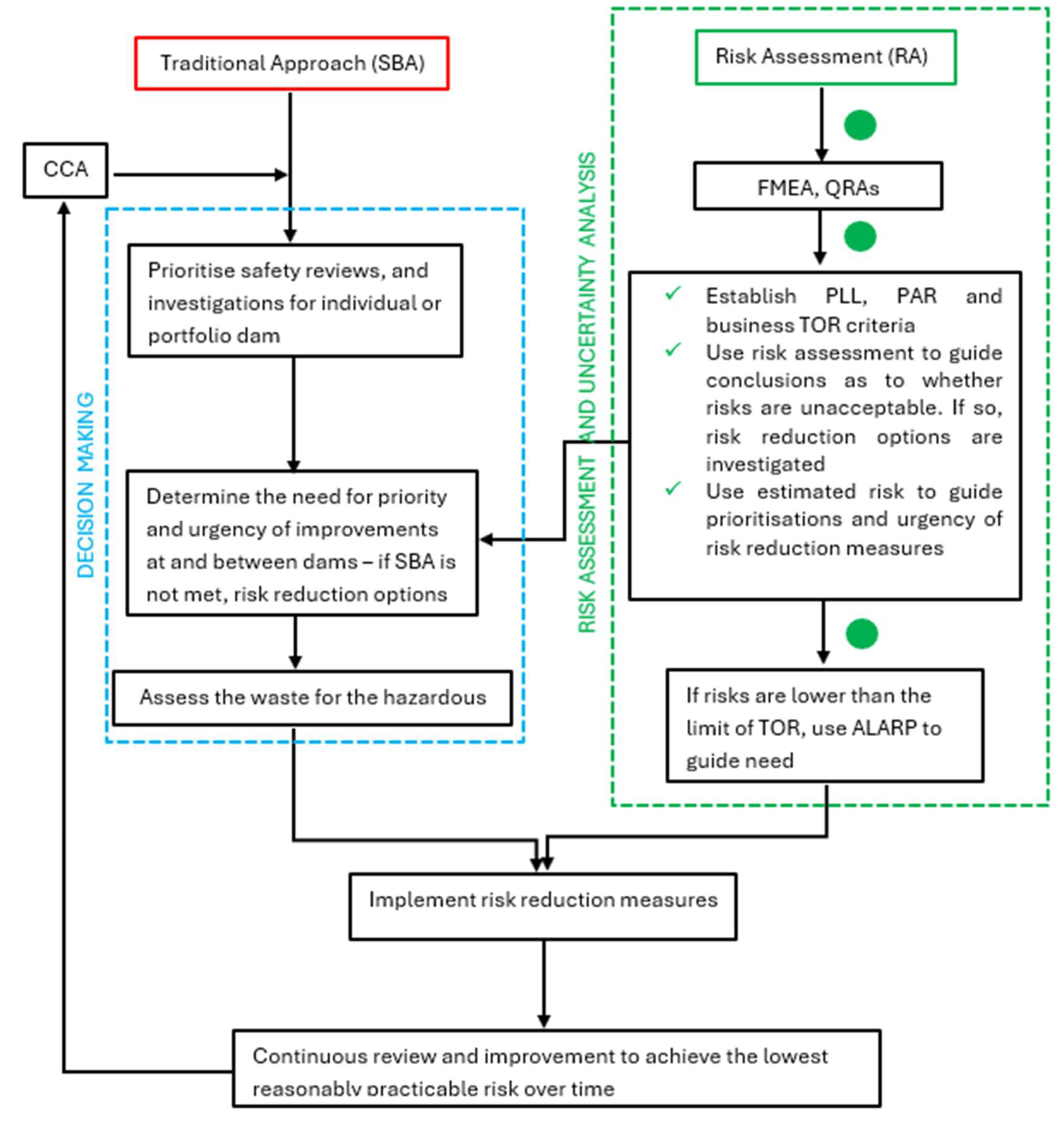
Risk analysis for dam safety is fundamentally a characterisation of the uncertainties in the performance capability of dams under loading conditions of interest. (Hartford & Baecher, 2004) including hazard and consequence analysis (Fell & Ho, 2005), and the effect of uncertainty on design objectives. Risk analysis in tailings dams is primarily conducted through a standards-based approach that considers the consequence category as a risk-based approach. However, other guidelines recommend that it be used only to inform the selection of design criteria and not as a measure of risk. According to ANCOLD (ANCOLD, 2022), the consequence category should be enhanced by a risk assessment to implement risk reduction measures (RRMs), as shown in Error! Reference source not found.. The adopted figure has been revised to reflect the critical components of risk assessment, uncertainty analysis, and decision-making in consequence-based analysis to enable risk-informed decision-making (RIDM). RIDM builds upon failure modes analysis, leveraging risk assessments to attain RRMs that meet ALARP. The consequence risk assessment should characterise the following to assist decision-making.
- lives lost
- tolerability of risk
- acceptability of risk, and
- as low as reasonably practicable (ALARP)
Figure 1.
Risk assessment as an enhancement of the standards-based or traditional approach showing locations of the flowsheet (green dots) where uncertainty analysis can be implemented to improve decision-making (adapted (ANCOLD, 2022).
Figure 1.
Risk assessment as an enhancement of the standards-based or traditional approach showing locations of the flowsheet (green dots) where uncertainty analysis can be implemented to improve decision-making (adapted (ANCOLD, 2022).
Vick (Vick et al., 1985) assets, the risk analysis of tailings dams should be probabilistic, which is also alluded to by ANCOLD, and all primary sources of uncertainty should be identified and classified. Once classified, sensitivity analyses should be conducted to test the uncertainty in the design input random variables, as well as other analysis methods such as Monte Carlo simulations (ANCOLD, 2022). Uncertainty analysis improves confidence levels in meeting tolerable risk guidelines, which can be applied to satisfy quantitative safety criteria as acceptable. Whitman (Whitman, 1984), suggested four requirements to satisfy acceptability. These include:
- criteria must be logical and understandable;
- criteria must be reasonable and acceptable methods of demonstration;
- criteria must have more risk reduction capabilities than the current practice; and
- implementation and imposition of criteria must be economical.
Tailings dams are characterised by complex uncertainties from different sources associated with the design, construction and operational phases of the life of a tailings facility (Klohn, 1972; McLeod et al., 2003; Ramon). These complexities are not considered explicitly in practice, and hence, the associated risk
2.4. Uncertainty in the Tailings Dam Design Process and Risk Analysis
The design process for tailings dams considers multivariate inputs often associated with inherent and transformational uncertainties. Since most design practices are based on guidelines that dictate the use of deterministic procedures (Vick et al., 1985). Recent tailings dam failures indicate that over-reliance on the prescribed values and procedures is not adequate to eliminate failure (Morgenstern, 2018). Primary sources of uncertainty are material strength parameters due to material variability and measurement errors in laboratory and field tests. Defining probability distribution functions (PDF) for design input variables, i.e. cohesion and friction, allows for the results to be interpreted with PDF, i.e. factors of safety, instead of a single value, which aids in decision-making and quantification of the effects of uncertainty. However, accurate construction of PDFs for design input variables is difficult due to the degree of variability and unknown uncertainty (Riddolls & Grocott, 1999).
Other design input data, such as maximum design flood (MDF), are characterised by uncertainty (Drobot et al., 2021). Some best distributions for empirical data might be unknown and are dynamic due to aleatory uncertainty due to variability, and length of available maximum discharge series, incomplete knowledge and climate change (Hoffman & Hammonds, 1994; Merz & Thieken, 2009). Merz and Thicken (Merz & Thieken, 2009) further explain why choosing the distribution function is a significant source of epistemic uncertainty in flood analysis, which is a critical component of risk assessment in the consequence-based approach.
The Nuclear Research Council (NRC, 1985) proposed a criteria for setting dam safety standards by following the approaches below (Stedinger et al., 1996):
- the deterministic probable maximum precipitation (PMP)/probable maximum flood (PMF) requires that structures be able to survive the estimated PMF;
- the structure probability of failure does not exceed a standard set for a failure mode or set of failure modes; and
- quantitative risk analysis procedures should be applied to quantify both probabilities of extreme hydrologic events and the consequences and incremental damage from the passage of the floods.
Stedinger’s report (Stedinger et al., 1996) further explains some of the issues with the results obtained by following the above approach, the considerations and the complexity of the analyses, and the acceptability of the approach, concluding that the impact of many factors that contribute to the probability of dam failure and magnitude of damage should be considered in risk analysis. The uncertainty of key design input parameters can be integrated by assigning probabilities.
The application of the consequence-based approach in risk quantification is empirically based on failure case histories (Feinberg et al., 2016), which implies that differences in failure case history, geographic location, topography, climate and seismic conditions might not apply globally. However, since the approach is widely accepted across the dam industry, risk analysis and quantification of tailings dams might be compromised on the premise of the character of the probability information used to determine the risk (Borovcnik, 2015).
Baecher(Baecher & Christian, 2005), discusses the role of uncertainty in risk analysis, defining three main uncertainty types that contribute to risk analysis: natural variability (temporal and spatial), knowledge uncertainty (models and input parameters) and decision model uncertainty (objectives, values, time preferences). Reviewing the current risk analysis methods and their influence on dam safety and decision-making (Fluixá-Sanmartín et al., 2020) indicates some shortfalls. These shortfalls include:
- inclusion of temporal changes in the design criteria and risk analysis, i.e. effects of climate change on risk tolerability
- how risk should be treated on a time-dependent basis, not under the stationarity principle (Milly et al., 2008)
The risk analysis methods applied in the mining industry will be discussed in the following section, with a particular focus on tailings dams, introducing Bayesian networks (BNs) and how their capability to incorporate uncertainty analysis and conditional probabilities in risk analysis models and update model distributions through inference modelling can be successfully applied in the tailings dam design process.
3. Risk Analysis Methods in Tailings Dam Design
Risk analysis forms a critical component of the risk management framework, with a primary objective of risk quantification derived from evaluating consequences and likelihood. The risk analysis of any design depends on the quality of the information under consideration and the inherent uncertainties, which can be used to inform decisions. Kaplan and Garrick (Kaplan & Garrick, 1981) define risk as a combination of uncertainty and damage, leading to understanding risk sources and their magnitudes (Hartford & Baecher, 2004). Hartford (op. cit.) further defines the risk analysis process of a dam and elucidates how it reveals the performance of a dam and its components and sub-systems as an enhancement of the traditional methods.
There are three principal methods, namely the failure modes and effects analysis (FMEA) and the associated methods: the event tree analysis (ETA) and the fault tree analysis (FTA) (Association, 1991). These static analysis methods determine the hierarchical and sequential causation of failure. Other methods often utilised for risk analysis include bowties (BTA), fuzzy analysis (FA), and artificial intelligence and neural networks (ANN). These static risk analysis methods have also been utilised as hazard analysis methods (Zarei et al., 2017) in other industries.
Static logic risk analysis methods have limitations in analysing the dynamic and complex nature of tailings dams. Hence, other analysis methods, such as Bayesian networks, have gained popularity in recent years (Delgado-Hernández et al., 2014; George & Renjith, 2021; Khakzad et al., 2011; Pan et al., 2019; Sakar et al., 2021; Zhang et al., 2011), which will be discussed later in this paper.
3.1. Failure Modes and Effects Analysis Method (FMEA)
FMEA is a qualitative analysis that identifies a system's failure to function as intended (ANCOLD, 2022; APEGBC, 2016; Fell & Ho, 2005; Hartford & Baecher, 2004; Santos et al., 2012). It is a standard evaluation procedure and an inductive method of reliability analysis for identifying potential failures in a system design and analysing the effects on the performance of the equipment (Schüller et al., 1997). The FMEA, as a qualitative risk analysis method, is industry-accepted and widely used (Yazdi et al., 2019) for risk identification and system reliability evaluation, forming a critical step in the risk analysis framework shown in Error! Reference source not found.. FMEA results are important input parameters to other risk analysis methods, such as FTA and ETA, and have been extended in their application to consider the criticality of the failure modes in the system. The failure modes and effects and criticality analysis (FMECA) enumerates the frequency of occurrence and consequences of each failure mode (Hartford & Baecher, 2004). Assigning a criticality aspect to a system’s component, such as tailings dams quantitatively, can be used to estimate the overall system reliability (Ruijters & Stoelinga).
Other variations of the FMEA have also been used in the dam industry, such as the potential failure modes analysis (PFMA), a subjective expert judgement conducted through elicitation. (DeNeale et al., 2019). PFMA involves the identification of potential failure modes under static loading, average operating water level, flood and earthquake conditions, including all external loading conditions for water retaining structures, and the assessment of those potential failure modes of enough significance to warrant continued awareness and attention to visual observation, monitoring and remediation as appropriate.
3.2. Event Tree Analysis (ETA)
Event trees are applied mostly in dam engineering as a mathematical tool for risk quantification (Phoon & Ching, 2018). ETA identifies the operating or failed states of a system and identifies events that require further analysis in a fault tree analysis (Hartford & Baecher, 2004). The ETA is an inductive risk analysis method that initiates from a specific system event to induce a general conclusion of its effect on the overall system performance.
3.3. Fault Tree Analysis (FTA)
Fault trees are widely used and accepted qualitative and quantitative risk evaluation methods in dam engineering. The risk analysis method was initially developed to evaluate the reliability and complex systems (Hartford & Baecher, 2004). Henrion (Henrion et al., 1991) defines a fault tree as an influence diagrams that exclusively express probabilistic relationships among system states without consideration of decisions and values. System relationships are expressed through deductive analysis, which postulates a system’s failure and attempts to deduce the mode and the failure sequence (Vesely et al., 1981). This paper focuses on the FTA method due to its prevalent use in tailings dam failure analysis during expert panel investigations. This is mainly due to FTA's ability to focus more on the events leading to the failure and design dependability (Ruijters & Stoelinga) compared to ETA, which describes all possible event combinations or factors.
In FTA analysis, system failure may or may not occur, and each system or sub-system is considered to be working or inoperable. Stedinger (Stedinger et al., 1996) argues that the narrow fault tree analysis framework and the general ETA make both methods unsatisfactory for detailed dam safety analysis. Hence, another paradigm is needed, which allows the analysis to include several continuous variables without discretising their probabilities. These shortfalls in the static logical methods can be alleviated through Bayesian networks (Bobbio et al., 2001), as discussed below.
The computing probability of a fault tree is solved through binary decision diagrams (BDD), which consider dependencies between nodes due to the redundancy of unfactorised events (Weber et al., 2012). Weber (2012) alludes that fault trees allow dependencies between events to be integrated with different knowledge backgrounds, i.e., technical, organisational, decisional and human aspects. However, fault trees have a shortfall in multiple state variables, which are usually associated with most tailings dam failures.
The static nature of fault trees in dynamic risk analysis requires the application of BNs, which use multi-modal logic with an unlimited number of modalities and make dependency analysis easier through DAGs.
Minimal Cut Set
A minimal cut set defines the basic events in a fault tree leading to the top event (failure) eventuation. The ranking of a cut set is a qualitative measure of subsystems and component failures leading to overall system failure (Ruijters & Stoelinga; Vesely et al., 1981). The quantitative measure deduces failure probabilities and also measures event importance to the probability.
Fault trees are characterised by primary, intermediate and top events. (Khakzad et al., 2011; Ruijters & Stoelinga; Vesely et al., 1981), with the top event defining the unwanted event or system failure. Primary events are assigned probabilities from historical systems’ performance data, monitoring data, or expert opinions, and they are linked to intermediate events by logic gates OR, AND, k/N, and INHIBIT gates. OR gate and AND gate are the most commonly used in dam engineering. Fault tree gates depict failure propagation through the system under analysis. Ruijters summarises the different methods used to determine the minimum cut set and how they provide information on systems’ vulnerabilities, which he alludes to as a good way to improve system reliability (Ruijters & Stoelinga).
3.4. Risk Tolerability and Acceptability
Once risk is analysed either qualitatively or quantitatively, a tolerability or acceptable criterion is determined for decision-making as part of the risk-informed decision-making approach. The risk tolerability concept was first introduced in Hong Kong in the 1970s (Morgenstern, 2018) and has since been developed through the years and adopted in the regulatory framework that governs dam design and decision-making (ANCOLD, 2022; CDA, 2013)
3.5. Bayesian Networks
Bayesian Networks (BNs) represent high-dimensional modelling using graph theory to model uncertainties and random variable dependencies. They are characterised by a directed acyclic graph (DAG) with conditional probability distributions, with nodes representing the random variable and the arcs the dependence relationship between nodes. Hence, they express a simplified representation of joint distributions and their dependencies.(Hanea et al., 2015; Oswaldo Morales-Nápoles & Juan Carlos, 2014) and provide a compact representation of high-dimensional uncertainty distributions of variables. BNs also encode the probability density or mass function on variables through the specification of conditional independence statements in the form of an acyclic directed graph and probability functions (Hanea, 2008). The DAG of a BN induces an ordering, generally non-unique, and stipulates that each variable is conditionally independent of all predecessors in the ordering.
BNs can be split into discrete, normal and non-parametric (Hanea et al., 2006). Discrete BNs specify the marginal distributions for source nodes and conditional probabilities for child nodes. However, they are not suitable for complex problems (Pan et al., 2019). Other disadvantages of discrete BNs are listed below (Hanea et al., 2006):
- Applications involving high complexity in data-sparse environments are severely limited by excessive assignment burden, which leads to rapid, informal and indefensible quantification;
- The marginal distributions can often be retrieved from data, but not the full interactions between children and parent nodes. The marginal distributions represent the most important information driving the modes, with dependence information less important. Hence, the construction of conditional probability tales should not molest any available data;
- Discrete BNs take marginal distributions only for source nodes; marginals for other nodes are computed from the conditional probability nodes. When these marginals are available from data, difficult constraints on the conditional probabilities are imposed. Quantifying with expert judgment would be impractical to configure the elicitation such that the experts would comply with the marginals.
Normal BNs restrict the joint normal distribution, and in the absence of data, experts can estimate partial regression coefficients and conditional variances.
Non-parametric BNs (NPBNs) were introduced as distribution-free continuous belief nets using a vines-copulae modelling approach (Kurowicka & Cooke, 2005). NPBNs were developed for purely continuous BNs (Hanea et al., 2015). In this approach, nodes are associated with arbitrary continuous invertible distributions, and influences are associated with (conditional) rank correlations and are realised by (conditional) copulae. Hence, no joint distribution is assumed, making the BN non-parametric (Hanea et al., 2006). To quantify BNs using this approach, all one-dimensional marginal distributions and some rank correlations equal to the number of arcs in the BN must be specified. Marginal distributions can be obtained through experts through Expert Panels and review boards for tailings dams.
Fault trees and event trees, which are mathematical models often applied in the tailings design process, rely on parameters whose values cannot be perfectly measured, with assumptions that uncertainties are independent. The inherent uncertainties in the input design parameters may be interrelated and dependent on each other. This is typical in the accident analysis using fault trees, which is often used to determine failure trigger mechanisms during expert panel reviews of tailings failures. Ignoring these dependencies may lead to large errors (Morales et al., 2008), particularly when designing dam structures, since dependence assumptions have been proven to influence both the average and output variability (Cortés et al., 2013). The copula-Bayesian approach (Pan et al., 2019) was applied when analysing the tailings dam failure discussed in Error! Reference source not found.Error! Reference source not found.Error! Reference source not found.Error! Reference source not found.Error! Reference source not found..
3.5.1. Copula-Based Models
Copulas allow the investigation of probabilistic dependence separately from the effect of one-dimensional marginals, hence their importance in the NPBN framework. The dependence function represented by the copula function is a cumulative joint distribution of correlated random variables. Dependence relationships are measured by the copula function, through Kendall’s tau (and Spearman’s rho ( correlation coefficients, which are used to estimate the parameters of bivariate copulas. The advantage of using Kendall’s ( over Spearman’s ( is the direct measure of the probabilities of observing concordant and discordant pairs (Zhang & Singh, 2019). Modelling copulas requires measured data to be transformed into a uniform distribution range of [0,1] through integration by parts at each node. The copula approach relies fundamentally on experts' ability to reliably assess random variable correlations. It defines the dependence between random variables by simplifying complex relationships into a marginal distribution, which enables the construction of multivariate distributions that satisfy non-parametric measures of dependence and prescribed marginal distributions.
Assuming a bivariate standard normal cumulative distribution function with Kendall correlation and the inverse of the univariate standard normal distribution function , the normal copula can be defined as below.
The relationship between the correlation of the normal copula (rank correlation of a normal variable) and the parameter (the product-moment correlation of the normal variables) can be represented as below (Kurowicka & Cooke, 2006; Morales et al., 2008);
Thus, any two random variables and can be joined by a copula if their joint distribution can be represented as below.
3.5.2. Dependability Analysis
Dependability analysis provides parameter prediction as an input for decision-making (Weber et al., 2012). Predictions through the failure probability models, such as remaining time to fail, mean time to failure (MTTF), mean time between failures (MTBF), repairable and unrepairable models, etc., provide quantitative failure and repair data associated with primary events. The application of BNs in risk analysis enables the evaluation of critical event occurrences such as tailings dam failures, where risk estimation or hazard occurrence depends on the reliability of the system components and human-system interactions.
Tailings dam failures require a systematic evaluation of causes, mechanisms and human-interaction aspects within a dynamic and evolving environment. Since tailings failure can be induced by low-probability events, the dependencies between variables become a critical aspect of analysis to aid decision-making.
Fault trees used for accident-cause analysis during expert reviews provide a tool that can be used and converted to BNs through mapping fault trees into BNs (Bobbio et al., 2001; George & Renjith, 2021; Khakzad et al., 2011). This paper focuses on risk assessment, system dependability, and the capability of BNs to make inferences on the fault tree and assess the reliability of the top event.
4. Methodology
UNINET is a stand-alone programme using Bayesian Belief Nets (BBNs) for stochastic modelling and multivariate ordinal data mining (Ababei, 2008). The software functions with other software packages, the graphic package UNIGRAPH and the sensitivity analysis program UNISENS. It can also be integrated with the uncertainty analysis program UNICORN, which will be discussed later.
4.1. Probabilistic Analysis
Probabilistic influences are represented by conditional rank correlation. The influence of the first parent on the child is assigned an unconditional rank correlation, and the influence of the second child is assigned a conditional rank correlation given the first parent. The conditional rank correlations are algebraically independent, i.e., previously chosen values do not constrain future choices. Thus, rank correlation is realised through the joint normal copula (Ababei, 2008).
4.2. Uncertainty Analysis
In uncertainty analysis, random variables are assigned a marginal distribution from a parametric distribution or user-defined distribution files. A DAG is specified to capture conditional relations, and parent-child probabilistic influences are represented as conditional rank correlation. Sequencing of conditional rank correlations implies that correlations are algebraically independent between -1 and 1, and contributes to the determinant of the BBN rank correlation matrix (DBBNR) (Kurowicka & Cooke, 2006). The DBBNR can be represented as below
If there are no arcs connecting parent and child nodes, . DBBNR reflects the conditional independence relations imposed by the BBN.
4.3. Analytic Conditioning
The distinctive feature of UNINET is its analytical conditioning capability. BBNs with numerous nodes can be conditionalised on arbitrary values of random variables, whereby the conditional distribution is computed quickly (Ababei, 2008), using the joint normal copula. Running the analytical conditioning mode allows UNINET to compute distributions of all functional nodes and build a joint density for all variables.
Analytical conditioning involves sampling the BBN, with options to define the number of samples used for creating the marginal distributions. It only applies to probabilistic nodes and conditionalising on interval values of functional nodes, and sample-based conditioning is applicable. Under sample-based conditioning, input and output nodes can be specified, with input nodes being conditionalised and output nodes indicating the effects of conditioning. Also, the unconditional and conditional means and standard deviation can be verified.
4.4. Assessing Model Adequacy
Model adequacy is defined by statistical measure of multivariate dependence. Testing whether the hypothesis for multivariate dependence on the joint normal copula should be rejected. This approach is based on “mutual information” as a measure of multivariate dependence (Ababei, 2008). The mutual information of a joint density , with marginal densities can be represented as below.
For a joint normal distribution, the mutual information is given by where is the mutual determinant of the correlation matrix. The determinant closely related to of the normal rank correlation matrix (DNR). To evaluate the suitability of a joint normal copula, the normal correlation matrix is compared with the empirical rank correlation matrix (DER) (Ababei, 2008). The DNR is also defined as the empirical normal determinant of the rank correlation matrix of the empirical normal version of as shown in Equation (3).
Where, denotes a joint normal distribution, normal variables with mean zero and unit variance. DER, on the other hand, is represented as below:
Where, denotes the determinant, which measures the amount of linear dependence between variables.
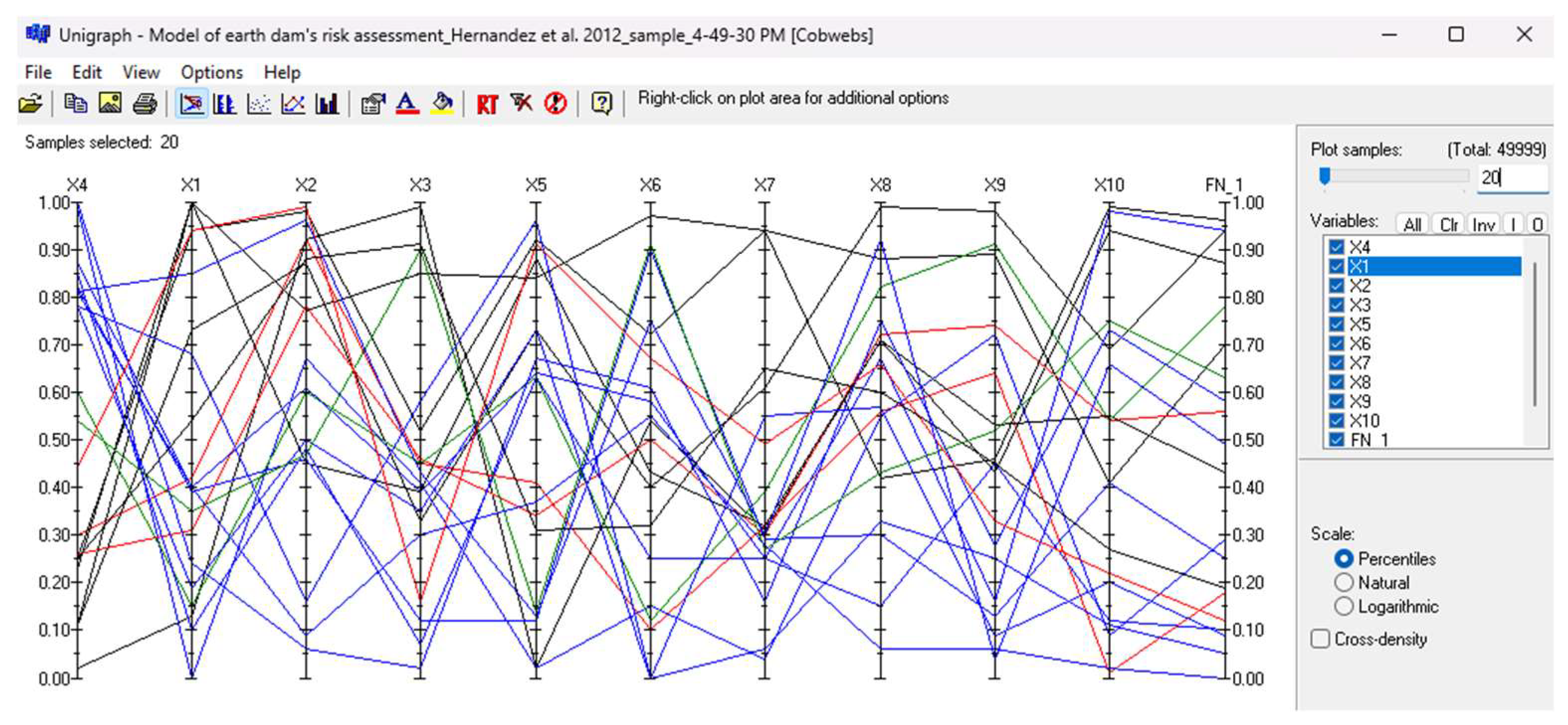
Once the model has been assessed for accuracy, results can be visualised in UNIGRAPH, a graphic package that supports visual analysis of multivariate distribution using cobweb plots. The graphical interpretation allows a visual representation of the joint distribution, with scatter plots, density plots, histograms and cobweb plots (Ababei et al., 2007). Cobweb plots represent variables as vertical lines (which can be presented on a percentile, natural, or logarithmic scale). Each sample is represented by one value of each variable. The lines are then connected by a segment, which is then visualised as a jagged line intersecting all vertical lines. Figure shows a typical cobweb plot showing multivariate dependence. The plot shows the percentiles of each variable and their relative dependence on the far-left variable, X4. If any two adjacent variables have the same corresponding percentile, then they will be perfectly rank correlated. Thus, the cross-density, the density of lines crossing on the midline between two adjacent vertical lines, will be concentrated in the middle, as shown in Figure for variables X4, X1, X2, X3, X4 and X5.
Figure 2.
Cobweb plot showing the representation of dependence of variables.
4.5. Mapping a Bayesian Network from a Fault Tree
Fault tree analysis is often conducted as a deductive accident analysis tool for tailings dams and is a widely accepted analysis tool in risk assessments. However, it is a static logic approach restricted to deterministic analysis. As a static risk analysis method, FT has limitations in dynamic risk analysis associated with complex systems such as tailings dams. However, these limitations can be alleviated through BNs (Bobbio et al., 2001). Fault tree mapping into a Bayesian network has been conducted in several studies (Bobbio et al., 2001; George & Renjith, 2021; Khakzad et al., 2011). Converting a fault tree (FT) into a Bayesian network (BN) enables the static information captured on the FT to be analysed to examine the influence of events (random variables) that contribute to the eventual failure of the dam. Variable dependencies and model risk assessment are also determined, and inference updating of prior probabilities can be conducted when new information is obtained. Applying this approach to tailings dam failure case histories enables accident analysis to determine the random variable dependencies, formulating risk assessment and uncertainty analysis models. These risk assessment models are useful in understanding risk profiles and aiding decision-making. The application of BNs acts as a predictive analysis tool, supporting the efficacy of the method in the design process for tailings dams.
Mapping an FT into a BN requires converting the logic binary nature into a marginal probability that can be assigned to each node based on the translation of the basic gate rules. The construction of the BN from an FT, through an equivalent node transfer from the FT, requires assigning marginal probabilities to parent nodes and conditional probabilities to the arcs to indicate the dependencies between nodes. The FT analysis involves qualitative and quantitative analysis, with the minimal cut set (MCS) computation representing the qualitative results. Minimal cut sets provide unique combinations of events that cause system failure as the prime implicants of the top event (TE). They define a combination (intersection) of primary events sufficient to cause the top event, which implies that if one of the failures in the cut set does not occur, then the top event will not occur (Vesely et al., 1981), at least in combination with the event not occurring. After combining the MCS, the importance factors can be obtained by ordering the MCS according to size.
Transferring an FT to a BN is achieved through an equivalent node transfer, which involves assigning marginal probabilities to parent nodes, directional arcs, and conditional probabilities to indicate the dependencies between nodes. Marginal and conditional probabilities transform the model to be analysed for random variable (event ) dependencies. The model can also be used for predictive analysis, risk assessment, uncertainty analysis, prior probability updating and data inference. The model can also be used for optimised design input parameter screening and uncertainty reduction for the tailings dam design process. The case study in this paper will be analysed using this approach.
The Top Event Fault Tree Analysis (TEFTA) software (Reliotec, 2024) was used to analyse the FT from the expert panel reports. TEFTA applies the following Boolean logic gates to indicate relationships between events.
5. Case Study
5.1. Mt Polley
The events leading to the cause of the structural failure were subdivided into proximate causes, root causes, and failed or defeated controls (Mines, 2014).
Proximate causes leading to the failure included:
- Breach of the dam;
- Structural failure of embankment:
- a.
- Uncharacterised weak upper glaciolacustrine clay unit (UGLU)
- b.
- Buttress sub-excavation
- c.
- Embankment geometry
- Beaches and supernatant water:
- d.
- Insufficient beaches
- e.
- Too much supernatant water
Root causes included:
- No long-term planning;
- No qualified responsible person;
- No site integration
Failed or defeated controls included:
- Inadequate water management plan
- Discharge permit process
- Ministry of Energy and Mines (MEM) query discounted (2006)
Events were rearranged in TEFTA, and a probability function was assigned based on expert opinions. Failure probability model functions in Table were used to assign probabilities to the events based on the root cause analysis (RCA). The Mt Polley FTA models used for modelling are shown in Table Error! Reference source not found..
Table 2.
Fault tree gates in TEFTA.
| Gate | Causal relation | Boolean Function | Number of inputs |
|---|---|---|---|
OR
|
The OR gate is used to indicate that the output occurs if at least one of the input events occur | 2 or more | |
AND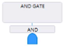
|
The AND gate is used to indicate that the output occurs if all the input events occur | 2 or more | |
VOTING
|
The VOTING gate is used to indicate that the output occurs if at least n out of the m input event occurs | when three inputs (a, b and c) and n = 2 | 2 or more |
INHIBIT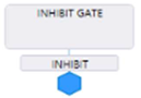
|
Inhibit gates are a special type of gate that must have exactly two inputs. One of the inputs is normally a conditioning event representing a probability. This gate is assumed to be an AND gate by fault tree quantification | 2 | |
NOT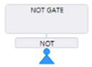
|
The NOT gate is used to indicate that the output occurs only when the input event does not occur | 1 | |
NOR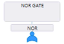
|
The NOR gate is used to indicate that the output occurs when all of the input events are absent | 2 or more | |
NAND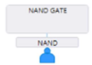
|
The NAND gate is used to indicate that the output occurs when at least one of the inputs is absent | 2 or more | |
XOR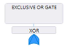
|
The EXCLUSIVE OR gate is used to indicate that the output occurs if one of the two input events occurs and the other input event does not occur | 2 | |
TRANSFER
|
The TRANSFER gates separate the fault tree (sub-tree) |
Table 3.
Mt Polley probability function derivation for modelling.
| Name | Description | Function | Unit |
|---|---|---|---|
| Structural failure | Constant( q=0.001, w=0 ) | Hour | |
| Weak UGLU not characterised | The inadequate site investigation (initial in 1996) influenced the stability analysis of the dam structure | MTTF( MTTF=18 ) | Year |
| Buttress excavation | Existence of unfilled foundation excavation, approximately 2 m or more in depth, extending from the toe of the embankment outward to approximately 20m, along the length of the Perimeter Embankment (PE). Excavation was done in November 2013 | MTTF( MTTF=9 ) | Month |
| Embankment geometry too steep for height | On July 28 and 29, 2014, Zone C rockfill was placed at the breach site to an elevation of 969.0 m | MTTF( MTTF=15 ) | Day |
| Insufficient beaches | Starting in 2011 (Stage 7, rises in pond elevation hampered the ability to maintain tailings beaches | MTTF( MTTF=38 ) | Month |
| Too much supernatant water | The mine had ample warnings. Indicators as early as February 2004 indicated a growing urgency of water discharge planning | MTTF( MTTF=10 ) | Year |
| Perimeter Embankment design section moved | Constant( q=0.001, w=0 ) | Hour | |
| Engineer of record (EoR) changeover (2011) | MTTF( MTTF=3 ) | Year | |
| DSR (2006) | Constant( q=0.001, w=0 ) | Hour | |
| MEM query discounted | Constant( q=0.001, w=0 ) | Hour | |
| MEM request discounted (KP 2005, AEC 2012) | Constant( q=0.001, w=0 ) | Hour | |
| MEM request for additional dam boreholes (1995) | MTTF( MTTF=10 ) | Year | |
| TSF investigation inadequate for PE foundation | Constant( q=0.001, w=0 ) | Hour | |
| Engineer did not manage the risk | Constant( q=0.001, w=0 ) | Hour | |
| Engineer could not complete the inspection | In December 2013 the engineer attended the sub-excavation to inspect it prior to backfilling, he could not complete the inspection due to snowfall | MTTF( MTTF=8 ) | Month |
| EoR changeover not integrated | Constant( q=0.001, w=0 ) | Hour | |
| MEM not informed | MTTF( MTTF=9 ) | Month | |
| BGC consultants recommend MPMC construct PE buttress | MTTF( MTTF=10 ) | Month | |
| Engineering standards of practice | Constant( q=0.001, w=0 ) | Hour | |
| Professional reliance | Constant( q=0.001, w=0 ) | Hour | |
| Mistaken belief in FoS | Constant( q=0.001, w=0 ) | Hour | |
| Production priorities | MTTF( MTTF=1 ) | Year | |
| Logistics and limitations | MTTF( MTTF=1 ) | Year | |
| Demand for TSF capacity | MTTF( MTTF=1 ) | Hour | |
| Maintenance of beaches | Constant( q=0.001, w=0 ) | Hour | |
| Poor water management | MTTF( MTTF=1 ) | Year | |
| Discharge permit process | Constant( q=0.001, w=0 ) | Hour | |
| Water management plan inadequate | Constant( q=0.001, w=0 ) | Hour | |
| Uncontrolled water balance | MTTF( MTTF=1 ) | Year | |
| Model2 | MTTF( MTTF=9 ) | Month | |
| Model14 | Constant( q=0.001, w=0 ) | Hour | |
| Model16 | Constant( q=0.001, w=0 ) | Hour |
Model events were defined from the basic events, also called the lowest-level events or terminating events in this thesis. The basic events for the Mt Polley failure model are shown in Table .
Table 4.
Mt Polley model basic events description.
| Name | Type | Description | Model | Function |
| E2 | Basic | Production priorities | Production priorities | MTTF( MTTF=1 ) |
| E3 | Basic | Logistics limitations | Logistics and limitations | MTTF( MTTF=1 ) |
| E1 | Basic | Engineer could not complete the inspection (December 2013) | Engineer could not complete inspection | MTTF( MTTF=8 ) |
| E7 | Basic | Management oversight insufficient | Model2 | MTTF( MTTF=9 ) |
| E8 | Basic | EoR changeover not integrated | EoR changeover not integrated | Constant( q=0.001, w=0 ) |
| E9 | Basic | MEM not informed | MEM not informed | MTTF( MTTF=9 ) |
| E10 | Basic | BGC recommends that MPMC construct a PE buttress (October 3, 2013) | BGC recommends MPMC construct PE buttress | MTTF( MTTF=10 ) |
| E11 | Basic | PE design section removed | PE design section moved | Constant( q=0.001, w=0 ) |
| E12 | Basic | EoR changeover (2011) | EoR changeover (2011) | MTTF( MTTF=3 ) |
| E13 | Basic | DSR (2006) | DSR (2006) | Constant( q=0.001, w=0 ) |
| E14 | Basic | MEM query discounted (KP 2005 / AMEC 2012) | MEM query discounted | Constant( q=0.001, w=0 ) |
| E15 | Basic | MEM request for additional starter dam boreholes (1995) | MEM request for additional dam boreholes (1995) | MTTF( MTTF=10 ) |
| E16 | Basic | TSF site investigation inadequate for PE foundation | TSF investigation inadequate for PE foundation | Constant( q=0.001, w=0 ) |
| E17 | Basic | Professional reliance | Professional reliance | Constant( q=0.001, w=0 ) |
| E18 | Basic | Mistaken belief in FoS | Mistaken belief in FoS | Constant( q=0.001, w=0 ) |
| E4 | Basic | No long-term planning | Model14 | Constant( q=0.001, w=0 ) |
| E5 | Basic | No qualified person | Model2 | MTTF( MTTF=9 ) |
| E6 | Basic | No site integration | Model16 | Constant( q=0.001, w=0 ) |
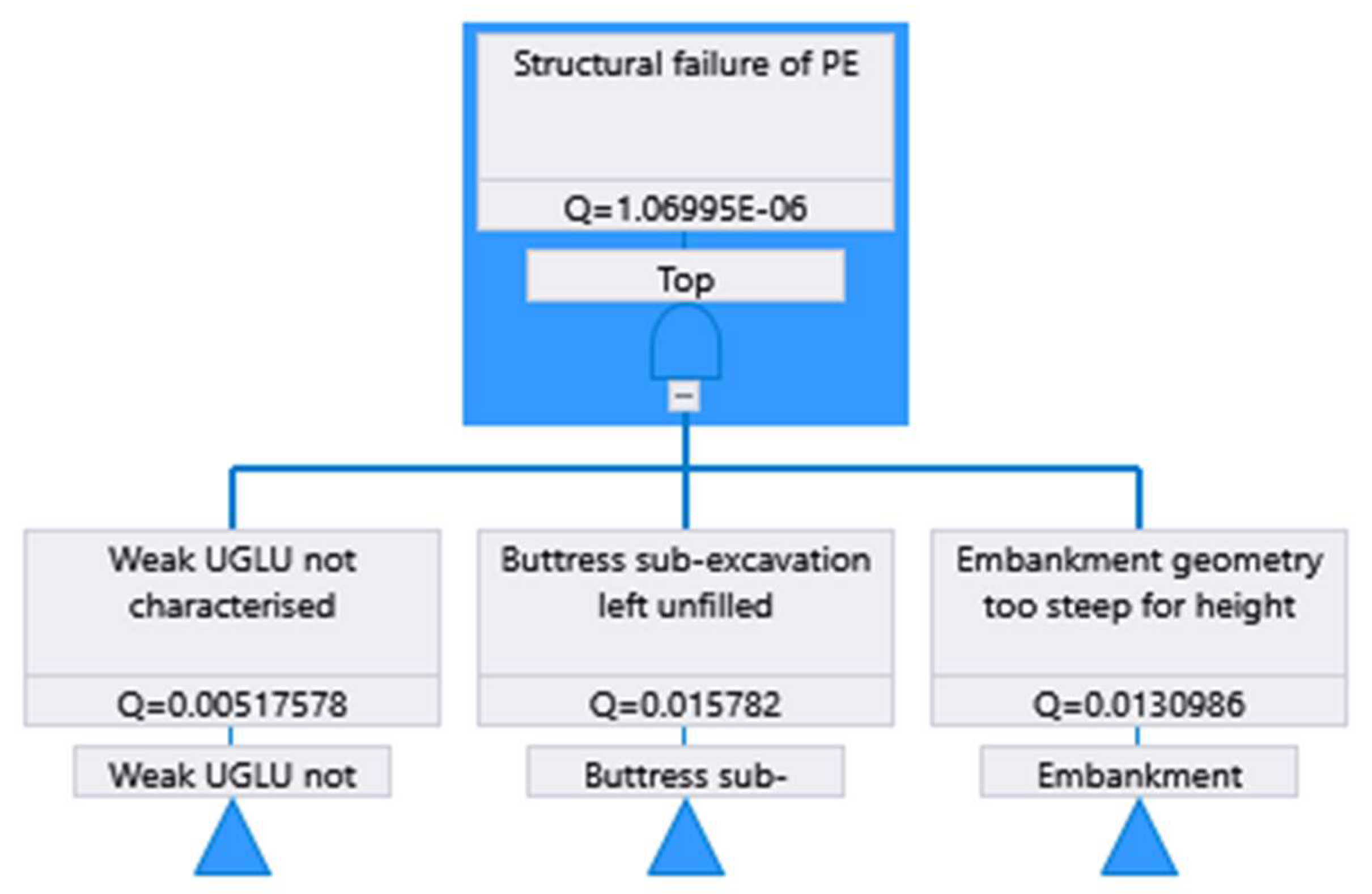
Based on the above analysis, the probabilities and the minimal cut set (MCS) for each of the three proximate causes that led to the structural failure of the Mt Polley perimeter embankment are tabulated below, Table to Table . The results indicate that the minimal cut sets contributing most to the failure were attributable to human aspects. Assessing the top event, the structural failure of the perimeter embankment, the fault tree probability of the event occurring due to the proximate causes listed above was 1.07E-06. The probabilities of the proximate events were 5.18E-03 for uncharacterised weak UGLU, 1.58E-02 for buttress sub-excavation left unfilled, and 1.31E-02 for embankment geometry. Figure shows the FTA for Mt Polley perimeter embankment failure.
Table 5.
Uncharacterised weak upper glaciolacustrine clay unit.
| Minimal cut set | Probability | Critical Importance Factor | % contribution |
| E11 | 0.001 | 0.1924 | 19.3 |
| E13 | 0.001 | 0.1924 | 19.3 |
| E14 | 0.001 | 0.1924 | 19.3 |
| E16 | 0.001 | 0.1924 | 19.3 |
| E12 | 0.000913 | 0.175991 | 17.6 |
| E15 | 0.00027 | 0.0528143 | 5.3 |
Table 6.
Buttress excavation.
| Minimal cut set | Probability | Critical Importance Factor | % contribution |
| E1 | 0.004158 | 0.261847 | 26.2 |
| E7 | 0.00369685 | 0.232807 | 23.3 |
| E9 | 0.00369685 | 0.232807 | 23.3 |
| E10 | 0.00332778 | 0.209565 | 21.0 |
| E8 | 0.001 | 0.0629743 | 6.3 |
Table 7.
Embankment geometry too steep.
| Minimal cut set | Probability | Critical Importance Factor | % contribution |
| E5 | 0.369685 | 0.279569093 | 28.0 |
| E2 | 0.00273598 | 0.206704828 | 20.7 |
| E3 | 0.00273598 | 0.206704828 | 20.7 |
| E4 | 0.001 | 0.075419376 | 7.5 |
| E6 | 0.001 | 0.075419376 | 7.5 |
| E17 | 0.001 | 0.075419376 | 7.5 |
| E18 | 0.001 | 0.075419376 | 7.5 |
Figure 3.
FTA top event for Mt Polley perimeter embankment.
The FT was converted to a BN using the methods discussed in the preceding sections. Each conditional probability linking the nodes was obtained by calculating the probability of the top event and repeating the FT analysis with and without the event. The directionality of the arcs was as suggested in the expert panel FT. Conditional probabilities for Mt Polley FT analysis are shown in Table .
Table 8.
Conditional probabilities of events contributing to the structural failure of the Perimeter Embankmen.
Table 8.
Conditional probabilities of events contributing to the structural failure of the Perimeter Embankmen.
| Event | Conditional probability |
| E1=0 | 0.0117 |
| E2=0 | 0.0104 |
| E3=0 | 0.0104 |
| E4=0 | 0.0121 |
| E4=0 | 0.0047 |
| E5=0 | 0.0020 |
| E6=0 | 0.0057 |
| E5=0 | 0.0094 |
| E6=0 | 0.0131 |
| E7=0 | 0.0121 |
| E8=0 | 0.0148 |
| E9=0 | 0.0121 |
| E10=0 | 0.0125 |
| E11=0 | 0.0042 |
| E12=0 | 0.0043 |
| E13=0 | 0.0042 |
| E14=0 | 0.0042 |
| E15=0 | 0.0057 |
| E16=0 | 0.0042 |
| E17=0 | 0.0121 |
| E18=0 | 0.0121 |
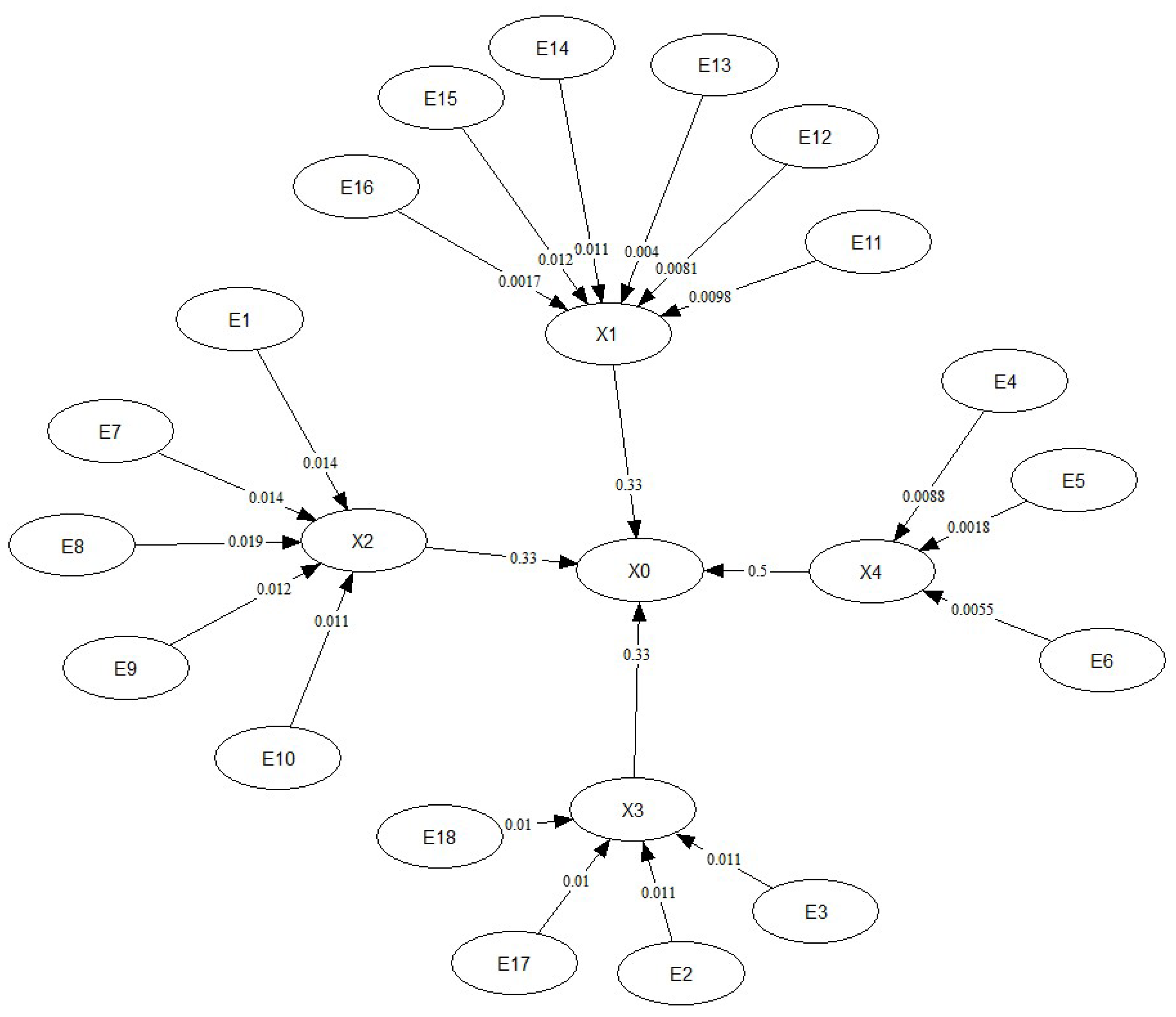
Based on the above analysis, a DAG was created showing the univariate random variables as per the FT and arcs indicating parent-child relationships. Conditional probabilities were assigned to the arcs according to Table . Since no marginal distributions are provided in the FTA, an assumption was made that all univariate distributions were transformed to be uniform distributions on (0,1). Hence, any copula could be used as long as it had an invertible cumulative distribution function. The DAG for the Mt Polley failure is shown in Figure . Each node's dependence information was rearranged to align with the sequence of events as reported in the expert panel report. The conditional probability of the proximal causes of the structural failure was assigned according to their contribution to the node, since they were not minimal cut sets. For example, since the proximal causes had an AND gate connecting them to the ultimate failure, the expert report stated that they both contributed to the structural failure. Thus, a conditional probability contribution of 0.33 was assigned. The same approach was also considered for the contribution of the uncontrolled water balance to the structural failure and embankment geometry.
Figure 4.
Mt Polley failure DAG for BBN sampling.

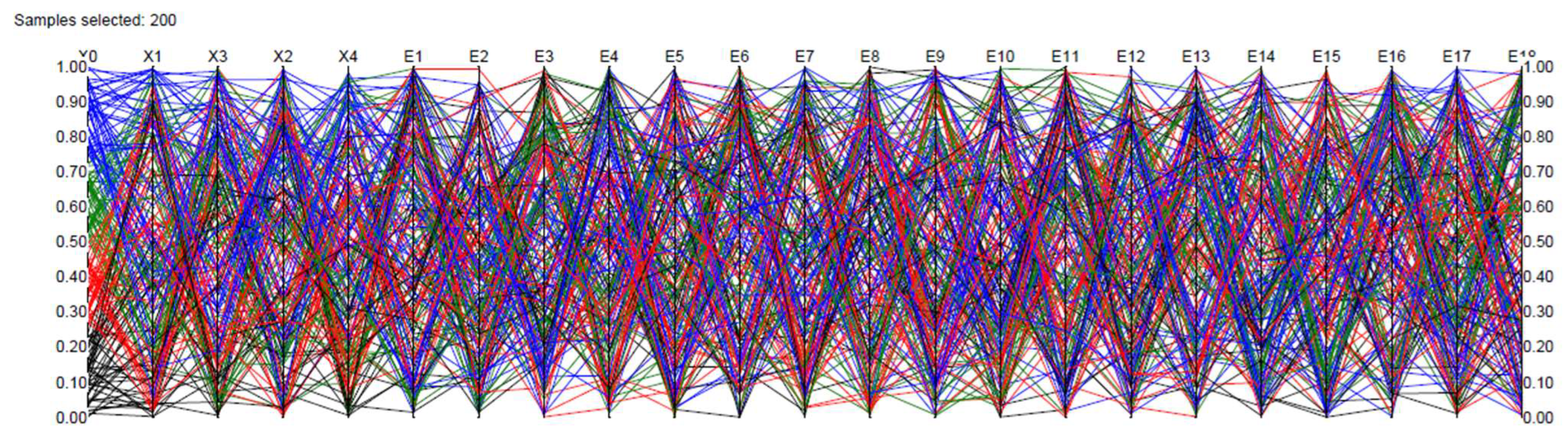
The BBN was sampled, and post-processed results were viewed in UNIGRAPH, a standalone package that processes results from UNINET. The results summarised the sampled model input and output data. UNIGRAPH plots a visual representation of the random variable’s joint distribution with cobweb plots. Cobweb plots represent variables with vertical lines, each sample representing a single value of each variable. By connecting through the percentiles, samples are presented as jagged lines intersecting the vertical lines. Figure shows a cobweb for the Mt Polley BBN model.
Figure 5.
Mt Polley failure BBN cobweb plot showing percentiles on the vertical axis.
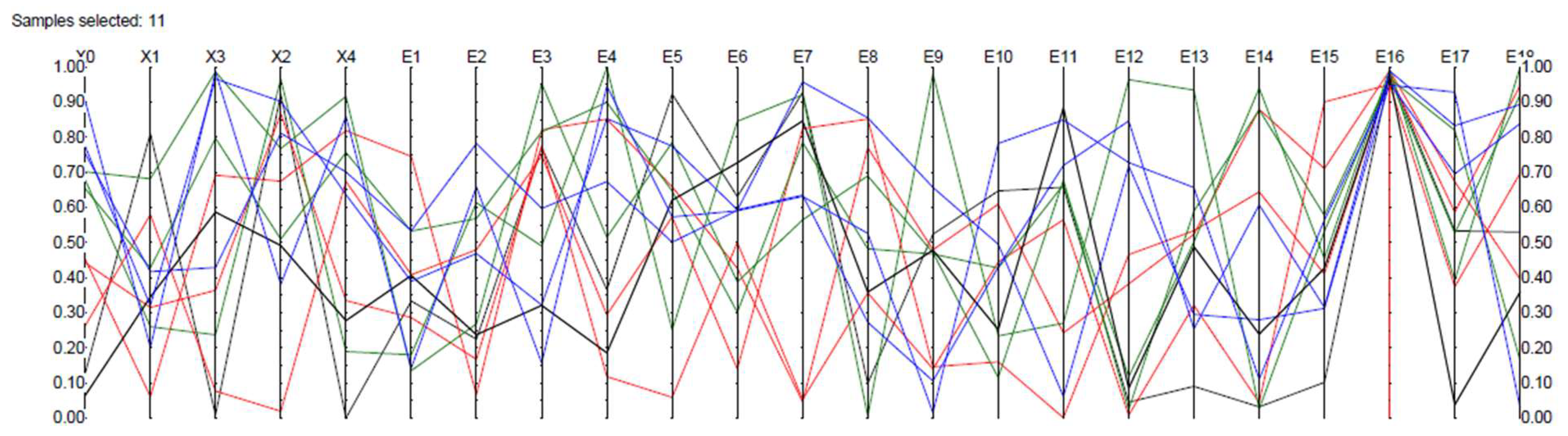
The cobweb plot allows the conditionalisation of variables to determine dependence. An example would be the assumption that high values of TSF site investigation inadequacy for the Perimeter Embankment significantly contributed to the structural failure. We can then determine its influence on other variables that led to the failure. Based on this background, assuming a distribution in the upper 5% of the distribution for E16, the results indicate that a positive dependence between E4, E7, X3, and X4 contributes approximately 90% of the percentile contribution to X0. However, this result also suggests a negative correlation between E16 and X1, as shown in Figure .
Figure 6.
Mt Polley cobweb plot conditionalised on the upper 5% of the TSF site investigation inadequate for PE foundation (E16) event’s distribution.
Figure 6.
Mt Polley cobweb plot conditionalised on the upper 5% of the TSF site investigation inadequate for PE foundation (E16) event’s distribution.
Model Accuracy
To check the accuracy of the BN model, the data function in UNINET was utilised. The suitability of a joint normal copula was evaluated by comparing the DNR with the DER. To show that the model is statistically acceptable, the rank correlation matrix (DBBNR) determinant was compared against the DNR. When the model was processed in data mining, the results showed a BN and correlations between variables slightly different to those shown in Figure . The generated correlated coefficients for the dataset are shown in Figure .
Figure 7.
Mt Polley failure conditional correlations generated by index sequencing on how the arcs were created.
Figure 7.
Mt Polley failure conditional correlations generated by index sequencing on how the arcs were created.
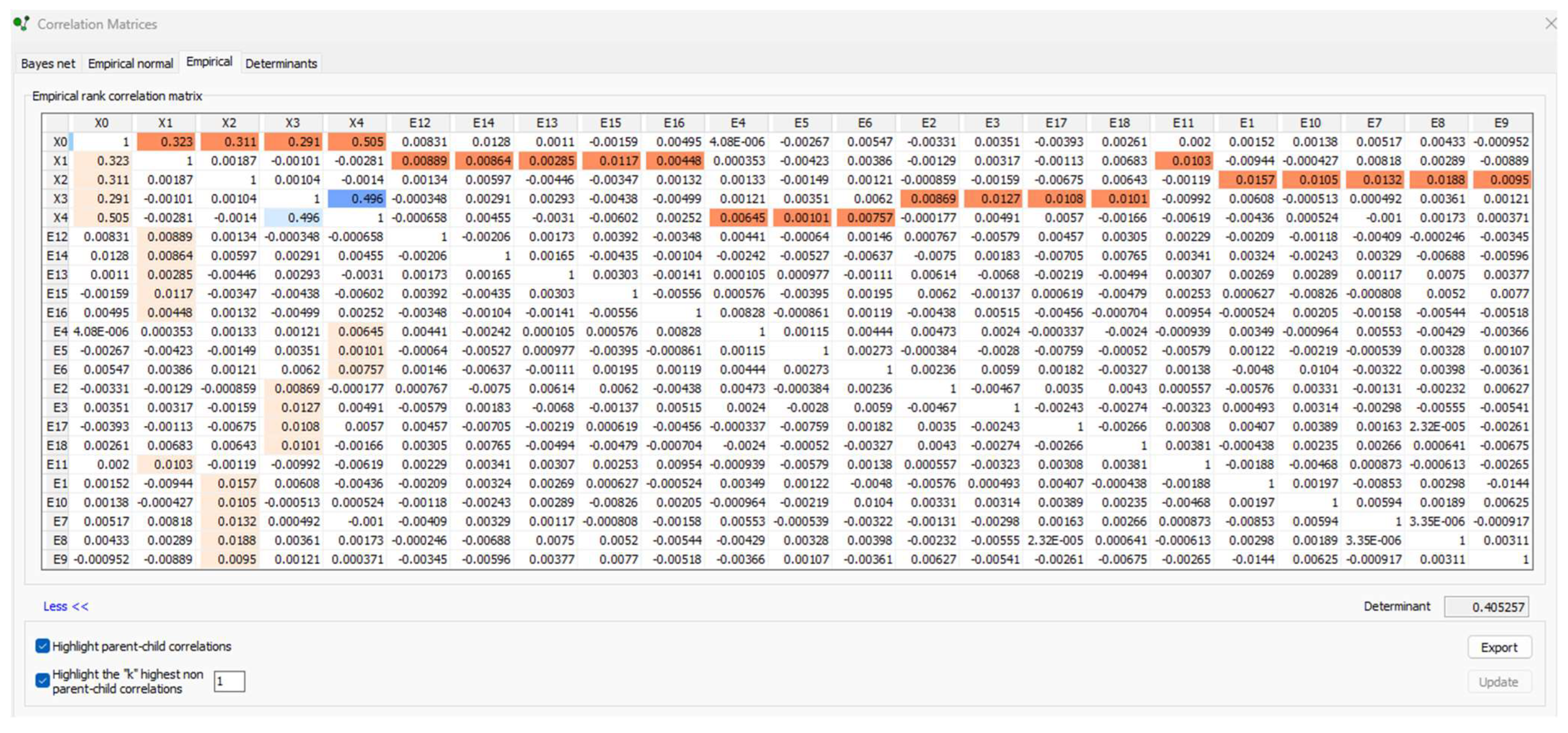
From the data, the correlation matrix determinants (DER, DNR and DBBNR) were analysed. Results indicated that DNR = 0.403849 was close to the DER = 0.405257. However, the DBBNR = 0.542429 determinant matrix was slightly higher, an indication that the model does not statistically represent the data. Figure shows the correlation matrices. To assess for missing interaction in the model, the correlations were compared using the software's compare correlation function. The “k” highest non-parent-child correlations indicated that X3 and X4 have a rank correlation in the empirical normal rank correlation matrix of 0.496, as shown in Figure . Adding the arc to link the two variables in the model and reprocessing the results, the determinants are comparable within the range, indicating that the model is now statistically representative of the data. The result also shows that the DBBNR would be predicted through approximation by using Equation (1), ich can be written as below:
Figure 8.
Correlation matrices, comparing DBBNR, DNR and DER for Mt Polley BBN model.
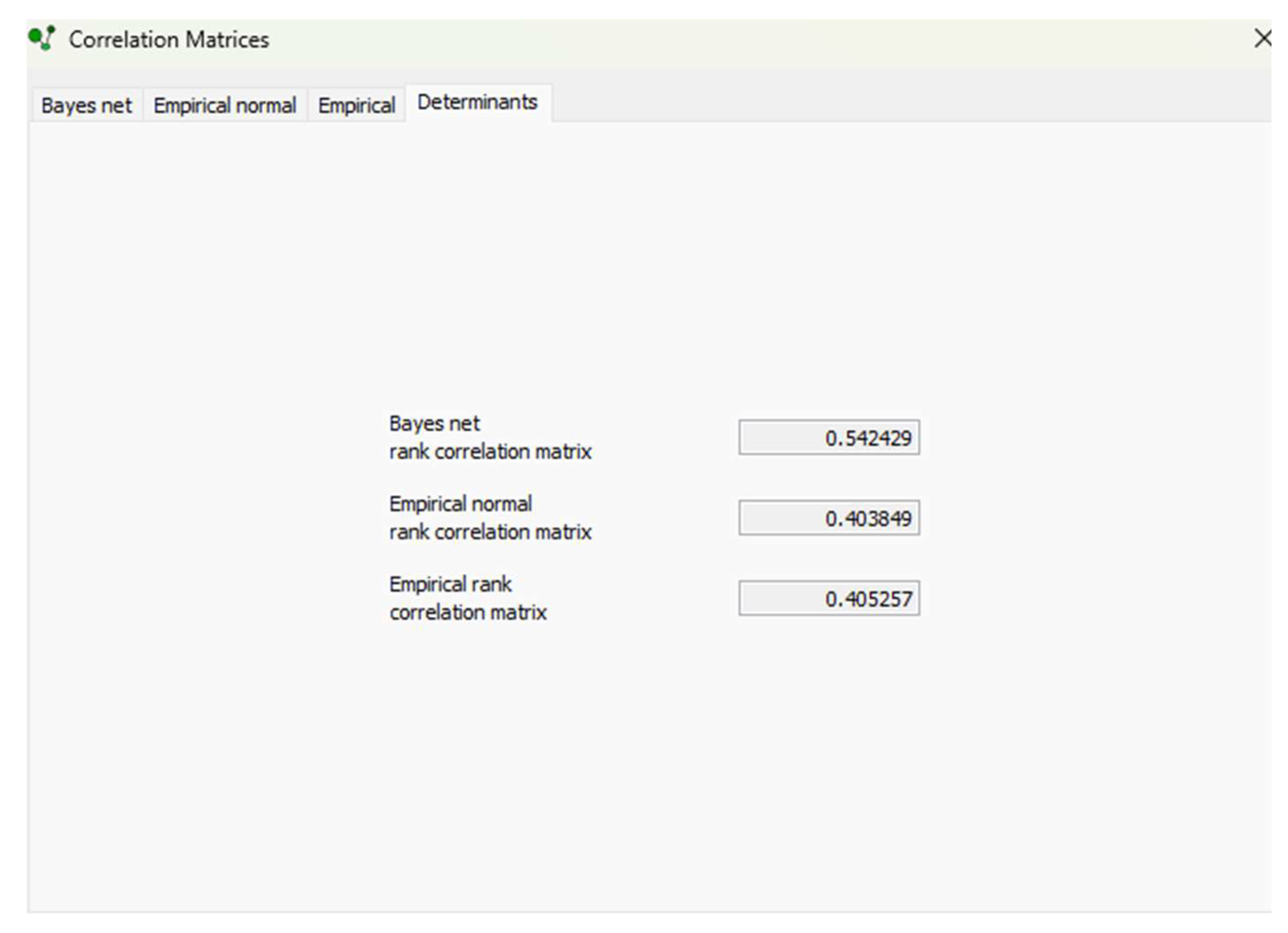
Figure 9.
Correlation matrices comparison showing the rank correlations between variables X3 and X4.
Figure 9.
Correlation matrices comparison showing the rank correlations between variables X3 and X4.
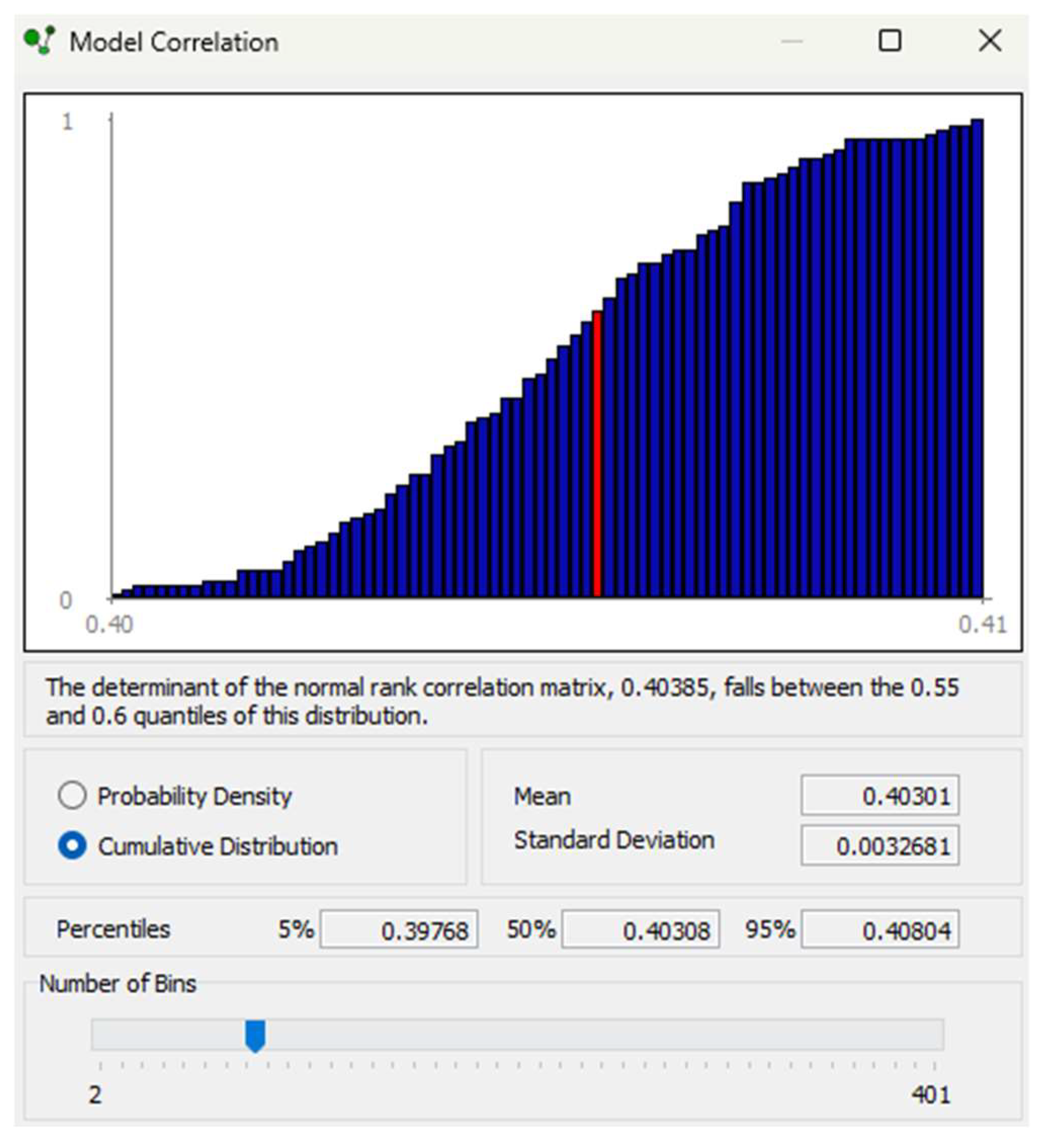
The corrected model and the correlation matrix determinants are shown in Figure and Figure . Validation of the model indicated that it was a good representation of normal data, with a 90% central confidence band of the determinant of the model's rank correlation matrix, as shown in Figure .
Figure 10.
Model showing arc connecting X3 and X4.
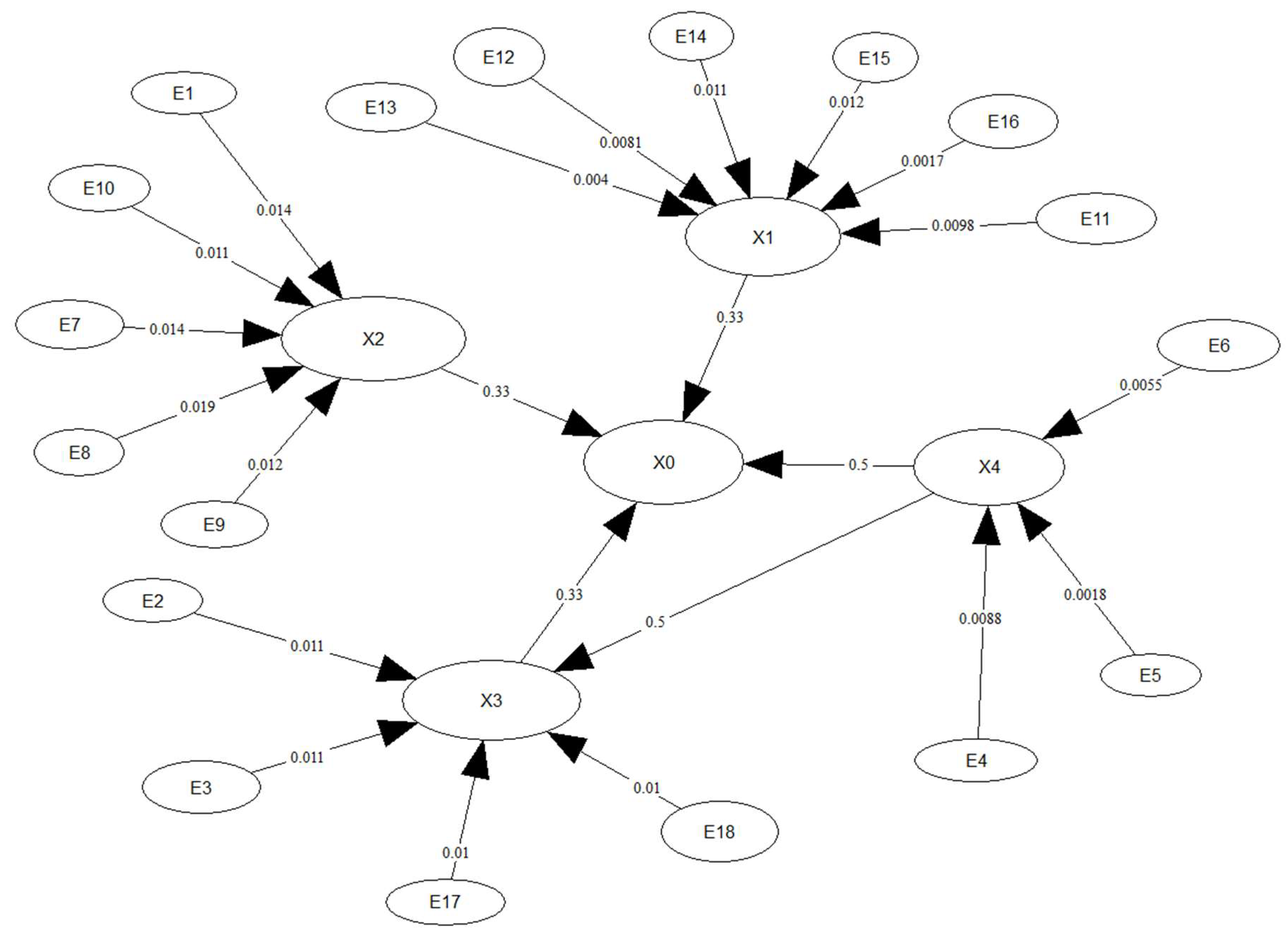
Figure 11.
Correlation determinants after directing the arc between X3 and X4.
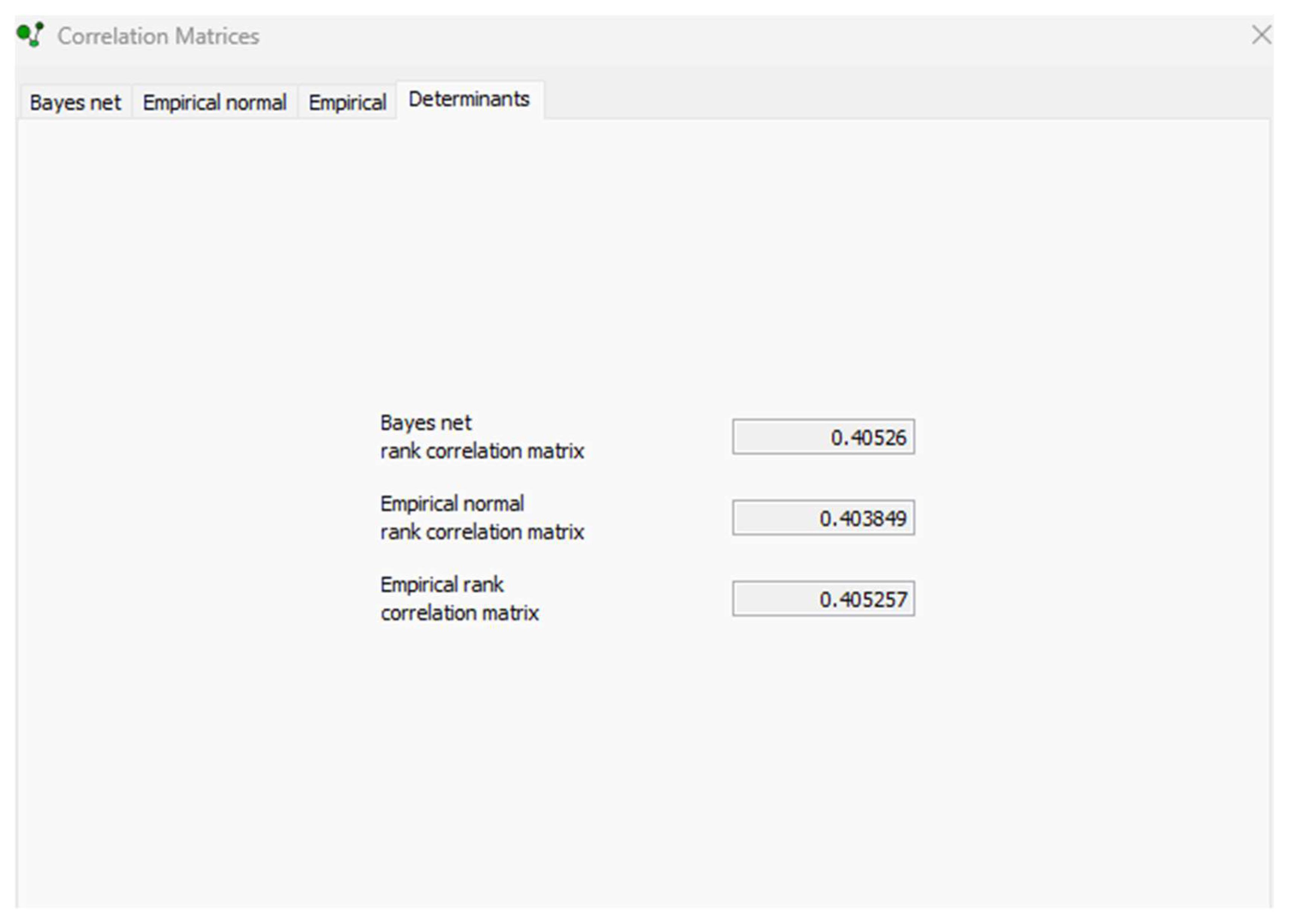
Figure 12.
Mt Polley model calibration results showing the cumulative distribution curve for the normal correlation matrix.
Figure 12.
Mt Polley model calibration results showing the cumulative distribution curve for the normal correlation matrix.
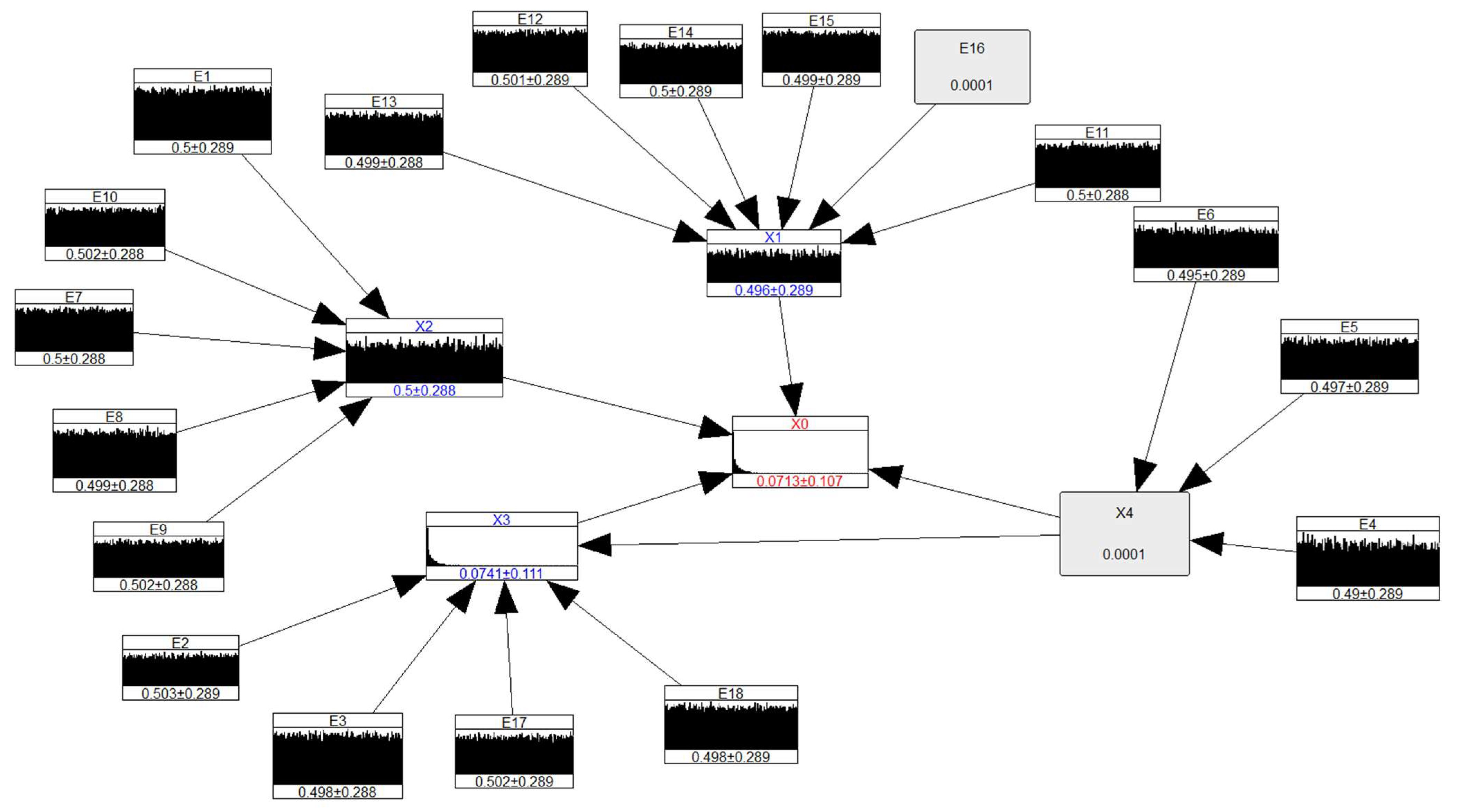
After model validation, the model could be used for evidence propagation for accident analysis or forward predictive analysis in the case of a new design. In the case of Mt. Polley, the model was used to determine the dependencies between variables for forensic accident analysis and to assess uncertainty. Conditionalising the structural failure of the Perimeter Embankment to a probability of 1×10⁻⁴, based on case histories of tailings dam failures, the contribution of other variables to the top event was determined. The BN was presented as histograms showing the means (conditional and unconditional) and standard deviations.
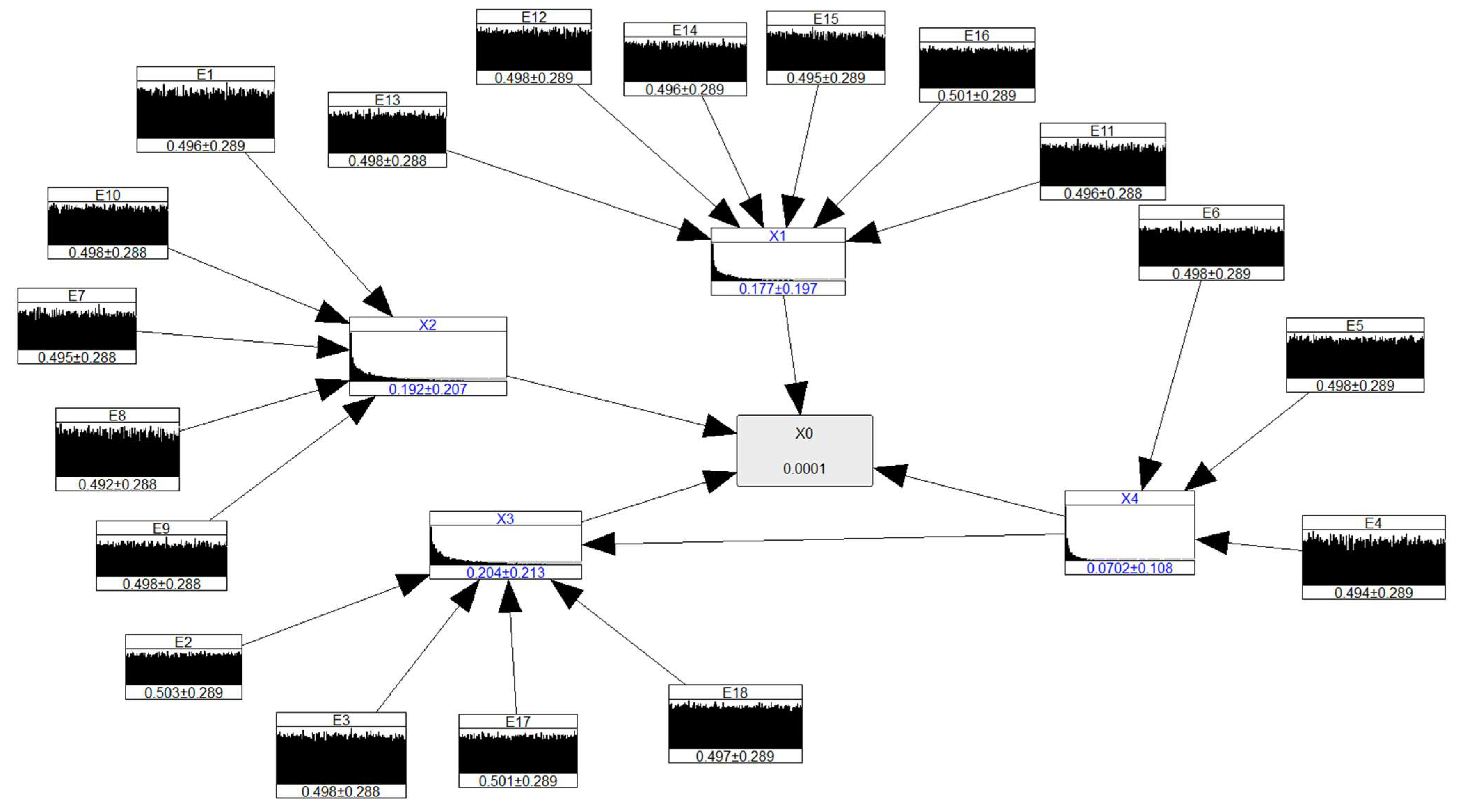
Figure shows the unconditional marginal distribution of the Mt Polley BBN. The effects of conditionalising the structural failure indicate that the variables X1, X2 and X3 are reduced to mean and standard deviation values of 0.20±0.20. However, X4 is significantly reduced to 0.07±0.11, as shown in Figure .
Figure 13.
Mt Polley BBN showing the unconditional marginal contributions with means and standard deviation shown below the histograms.
Figure 13.
Mt Polley BBN showing the unconditional marginal contributions with means and standard deviation shown below the histograms.
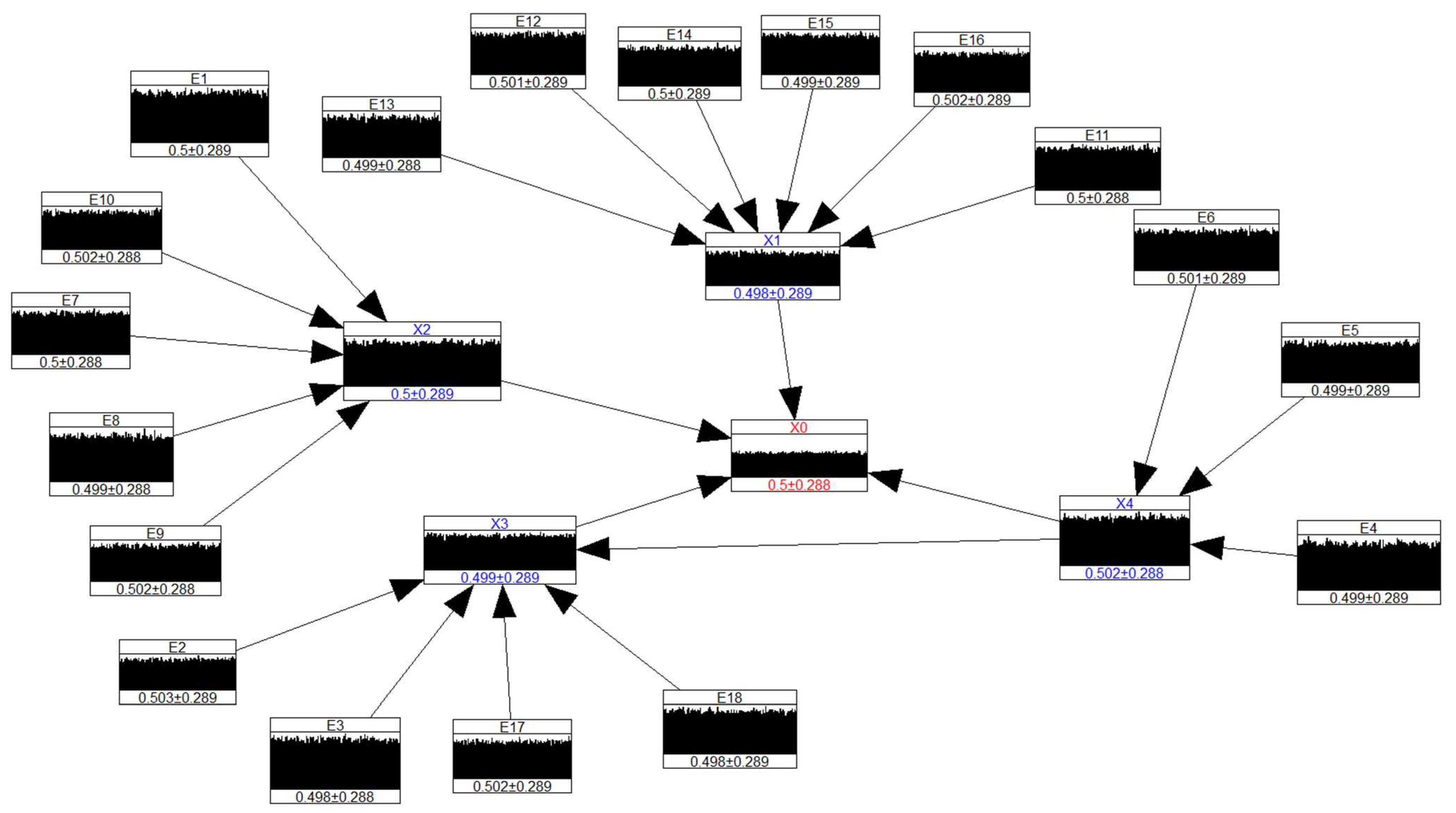
Figure 14.
Conditionalised BBN for Mt Polley, structural failure of the Perimeter Embankment reduced to a probability of 1×10⁻⁴.
Figure 14.
Conditionalised BBN for Mt Polley, structural failure of the Perimeter Embankment reduced to a probability of 1×10⁻⁴.
Conditionalising E16 and X4 by a magnitude of 10-4 reduced the occurrence of structural failure of the Perimeter Embankment significantly by 85% to a mean and standard deviation of 0.07±0.11. Figure shows the conditionalised BN.
Figure 15.
Conditionalised BBN for Mt Polley, E16 and X4 reduced to a probability of 10-4.
6. Discussion
The tailings design process, parameters, and risk assessment were reviewed with the following objectives:
- to describe the evolution of the current tailings design process and critique the design process; and
- evaluating the risk acceptability of the Mt Polley tailings dam failure, and its significant contribution to the governance and management of tailings dams.
The current design practice and risk assessment approaches were appraised and critiqued. A method to assess uncertainties associated with input design parameters was proposed, and its applicability was tested in target tailings dam failure case histories. The understanding of sources of uncertainties improves the confidence with which decisions can be made, and characterising how uncertainties can be addressed, represented and resolved can be a pathway to the acceptability of risk decisions.
7. Conclusions
The analysis of tailings dam design and risk assessment reveals a critical need for a more robust and comprehensive approach. Traditional deterministic methods and first-order probabilistic approaches, while useful, are fundamentally limited in their ability to handle the complexities and multifaceted uncertainties inherent in these systems. The reliance on a single factor of safety or the oversimplification of multi-variable dependencies can lead to a false sense of security and a failure to identify the true pathways to catastrophe.
The application of a Bayesian Network framework presents a powerful solution to these challenges. BNs provide a rigorous and transparent methodology for integrating a variety of data sources—from empirical test results to expert judgment—into a single, unified model. The framework's ability to explicitly differentiate between and quantify both aleatory and epistemic uncertainties is a key advantage. This distinction provides a clear, actionable guide for risk management, directing engineers to either invest in further data collection to reduce reducible uncertainty or to implement more robust design strategies to account for intrinsic variability.
Furthermore, the BN framework enables a holistic, systemic view of the tailings dam, moving beyond the isolated analysis of individual failure modes. The ability to model causal relationships and interdependencies between variables, such as the simultaneous impact of reservoir level on both overtopping and internal erosion risk, is a crucial step toward a more realistic risk assessment. As demonstrated in the retrospective analysis of the Mount Polley failure, a BN could have potentially identified the latent design flaws that went undetected by conventional methods, revealing a high-risk profile that would have warranted targeted investigation and proactive mitigation.
In conclusion, the industry must move beyond outdated methods and embrace the paradigm shift towards a more transparent, robust, and proactive approach to risk management. The Bayesian Network framework, particularly when extended with dynamic capabilities and integrated with real-time monitoring data, represents the most promising path forward. Its adoption has the potential to significantly enhance the safety and reliability of tailings dams and, most importantly, to prevent future catastrophic failures by fostering a culture of rigorous, risk-informed decision-making.
Acknowledgments
The author would like to thank the Geotechnical Engineering Centre (GEC) at the University of Queensland for the opportunity to research an exciting topic and for the support offered to supervise and direct my research programme. The research focused on the current design process and risk assessment of tailings dams, introducing Bayesian network analysis as a method that can be applied to enhance the design process and risk assessment methods. The rise of sustainability requirements, including environmental, social governance (ESG) and social responsibility (SR), has also motivated a change in the design process for tailings dams. This manuscript reviews the current practice and highlights some gaps that must be addressed to align with ESG/SR requirements, and introduces Bayesian network analysis as a method that can be applied to enhance the design process and risk assessment methods.
References
- Ababei, D. (2008). UNINET. In (Version 3.2). Available online: https://www.lighttwist.net/wp/uninet/.
- Ababei, D.; Kurowicka, D.; Cooke, R.M. (2007). Uncertainty analysis with UNICORN. Proceedings of the Third Brazilian conference on statistical Modelling in Insurance and Finance,.
- Allen, T. I., Griffin, J. D., Leonard, M., Clark, D. J., & Ghasemi, H. The 2018 national seismic hazard assessment of Australia: Quantifying hazard changes and model uncertainties. Earthquake Spectra 2020, 36(1_suppl), 5-43.
- ANCOLD (1998). Guidelines For Design of Dams For Earthquake. In.
- ANCOLD (2012). Guidelines on Tailings Dams–Planning Design, Construction, Operation, and Closure. In: ANCOLD Hobart, Australia.
- ANCOLD (2022). Guidelines on Risk Assessment. In (pp. 1-212): ANCOLD Inc.
- APEGBC (2016, October, 2016). Site Characterization for Dam Foundations in BC APEGBC Professional Practice Guidelines. APEGBC. Retrieved 08 August 2024 from. Available online: https://www.egbc.ca/getmedia/13381165-a596-48c2-bc31-2c7f89966d0d/2016_Site-Characterization-for-Dam-Foundations_WEB_V1-2.pdf.aspx.
- Association, C.S. (1991). Risk analysis requirements and guidelines: quality management-a national standard of Canada.
- Baecher, G. B., & Christian, J. T. (2005). Reliability and statistics in geotechnical engineering. John Wiley & Sons.
- Bobbio, A.; Portinale, L.; Minichino, M.; Ciancamerla, E. Improving the analysis of dependable systems by mapping fault trees into Bayesian networks. Reliability Engineering & System Safety 2001, 71, 249–260. [Google Scholar] [CrossRef]
- Borovcnik, M. Risk and decision making: The “logic” of probability. The Mathematics Enthusiast 2015, 12, 113–139. [Google Scholar] [CrossRef]
- Casagrande, L.; MacIver, B. (1970). Design and construction of tailings dams. Proceedings, Symposium on Stability in Open Pit Mining,.
- CDA (2013). Dam safety guidelines 2007. CDA, Ottawa.
- Committee, I.T.D. (2013). Sustainable design and post-closure performance of tailings dams (Bulletin 153). In: International Committee on Large Dams (ICOLD) Paris, France.
- Cortés, J.-C.; Romero, J.-V. ; Roselló; M-D; Villanueva, R.-J. (2013). Dealing with dependent uncertainty in modelling: a comparative study case through the Airy equation.
- Delgado-Hernández, D.-J.; Morales-Nápoles, O.; De-León-Escobedo, D.; Arteaga-Arcos, J.-C. A continuous Bayesian network for earth dams’ risk assessment: an application. Structure and Infrastructure Engineering 2014, 10, 225–238. [Google Scholar] [CrossRef]
- DeNeale, S. T. , Baecher, G. B., Stewart, K. M., Smith, E. D., & Watson, D. B. (2019). Current state-of-practice in dam safety risk assessment.
- Drobot, R.; Draghia, A. F. , Ciuiu, D., & Trandafir, R. Design floods considering the epistemic uncertainty. Water 2021, 13, 1601. [Google Scholar]
- Feinberg, B.; Engemoen, W.; Fiedler, W.; Osmun, D. (2016). Reclamation’s Empirical Method for Estimating Life Loss Due to Dam Failure.
- Fell, R. F. , & Ho, K. K. S. (2005). State of the Art Paper 1 A framework for landslide risk assessment and management.
- Fischhoff, B.; Lichtenstein, S.; Slovic, P.; Keeney, R.; Derby, S. (1980). Approaches to acceptable risk: A critical guide.
- Fluixá-Sanmartín, J.; Escuder-Bueno, I.; Morales-Torres, A.; Castillo-Rodríguez, J.T. Comprehensive decision-making approach for managing time dependent dam risks. Reliability Engineering & System Safety 2020, 203, 107100. [Google Scholar] [CrossRef]
- George, P. G. , & Renjith, V. Evolution of safety and security risk assessment methodologies towards the use of bayesian networks in process industries. Process Safety and Environmental Protection 2021, 149, 758–775. [Google Scholar]
- Hanea, A.; Napoles, O. M. , & Ababei, D. Non-parametric Bayesian networks: Improving theory and reviewing applications. Reliability Engineering & System Safety 2015, 144, 265–284. [Google Scholar]
- Hanea, A.M. (2008). Algorithms for non-parametric Bayesian belief nets.
- Hanea, A. M. , Kurowicka, D., & Cooke, R. M. Hybrid method for quantifying and analyzing Bayesian belief nets. Quality and Reliability Engineering International 2006, 22, 709–729. [Google Scholar]
- Hartford, D. N. , & Baecher, G. B. (2004). Risk and uncertainty in dam safety.
- Henrion, M.; Breese, J. S. , & Horvitz, E. J. Decision analysis and expert systems. AI magazine 1991, 12, 64–64. [Google Scholar]
- Hoffman, F. O. , & Hammonds, J. S. Propagation of uncertainty in risk assessments: the need to distinguish between uncertainty due to lack of knowledge and uncertainty due to variability. Risk analysis 1994, 14, 707–712. [Google Scholar]
- ICOLD (Ed.). (1988). Dam design criteria the philosophy of their selection Bulletin 061.
- Jansen, R.B. (1983). Dams and public safety. US Department of the Interior, Bureau of Reclamation.
- Kaplan, S.; Garrick, B.J. On the quantitative definition of risk. Risk analysis 1981, 1, 11–27. [Google Scholar] [CrossRef]
- Khakzad, N.; Khan, F.; Amyotte, P. Safety analysis in process facilities: Comparison of fault tree and Bayesian network approaches. Reliability Engineering & System Safety 2011, 96, 925–932. [Google Scholar] [CrossRef]
- Klohn, E.J. Design and construction of tailings dams. CIM Transactions 1972, 75, 50–66. [Google Scholar]
- Kurowicka, D.; Cooke, R. Distribution-free continuous Bayesian belief nets. Modern statistical and mathematical methods in reliability 2005, 10, 309–323. [Google Scholar]
- Kurowicka, D.; Cooke, R.M. (2006). Uncertainty analysis with high dimensional dependence modelling, John Wiley & Sons.
- MAC A Guide to the Management of Tailings Facilities. Version 3.1 2019, 96.
- McLeod, H.; Murray, L. ; BERGER; KC Tailings dam versus a water dam, what is the design difference.
- Merz, B.; Thieken, A.H. (2009). Flood risk curves and uncertainty bounds. Natural Hazards 2003, 51, 437–458. [Google Scholar] [CrossRef]
- Milly, P. C. , Betancourt, J., Falkenmark, M., Hirsch, R. M., Kundzewicz, Z. W., Lettenmaier, D. P., & Stouffer, R. J. Stationarity is dead: Whither water management? Science 2008, 319, 573–574. [Google Scholar] [PubMed]
- Mines, C.I. o. (2014). Investigation Report of the Chief Inspector of Mines. British Columbia Government. Retrieved 29/01/2025 from https://www2.gov.bc.ca/gov/content?id=16929E291845478AB33ED624BAF63A42.
- Morales, O.; Kurowicka, D.; Roelen, A. Eliciting conditional and unconditional rank correlations from conditional probabilities. Reliability Engineering & System Safety 2008, 93, 699–710. [Google Scholar] [CrossRef]
- Morgenstern, N.R. (2018). Geotechnical risk, regulation, and public policy.
- Oswaldo Morales-Nápoles, D.J. D.-H. D. D.-L.-E. , & Juan Carlos, A.-A. A continuous Bayesian network for earth dams' risk assessment: methodology and quantification. Structure and Infrastructure Engineering 2014, 10, 589–603. [Google Scholar] [CrossRef]
- Pan, Y.; Ou, S.; Zhang, L.; Zhang, W.; Wu, X.; Li, H. Modeling risks in dependent systems: A Copula-Bayesian approach. Reliability Engineering & System Safety 2019, 188, 416–431. [Google Scholar] [CrossRef]
- Phoon, K.-K. Uncertainty-Informed Decision-Making in Burland Triangle. In Uncertainty, Modeling, and Decision Making in Geotechnics (pp. 1-36). CRC Press.
- Phoon, K.-K.; Ching, J. (2018). Risk and reliability in geotechnical engineering. CRC Press.
- Ramon, V. Tailings dams. [CrossRef]
- Reliotec (2024) TopEvent, F.T.A. Retrieved 28/06/2024 from https://www.fault-tree-analysis.com/.
- Riddolls, B.; Grocott, G. (1999). Quantitative risk assessment methods for determining slope stability risk in the building industry. In: Building Research Association of New Zealand.
- Ruijters, E.; Stoelinga, M. Fault Tree Analysis: A Survey of the State-of-theart in Modeling. Analysis and Tools. Computer Science Review, 15-16.
- Sakar, C.; Toz, A. C. , Buber, M., & Koseoglu, B. Risk analysis of grounding accidents by mapping a fault tree into a Bayesian network. Applied Ocean Research 2021, 113, 102764. [Google Scholar]
- Santos, R.N.C. D. , Caldeira, L. M. M. S., & Serra, J. P. B. FMEA of a tailings dam. Georisk: Assessment and Management of Risk for Engineered Systems and Geohazards 2012, 6, 89–104. [Google Scholar]
- Schüller, J.; Brinkman, J.; Van Gestel, P. J. , & Van Otterloo, R. (1997). Methods for determining and processing probabilities: Red Book, Committee for the Prevention of Disasters.
- Stedinger, J. R. , Heath, D. C., & Thompson, K. (1996). Risk analysis for dam safety evaluation: hydrologic risk, US Army Corps of Engineers, Water Resources Support Center, Institute for ….
- Vesely, W. E., Goldberg, F. F., Roberts, N. H., & Haasl, D. F. (1981). Fault tree handbook. Systems and Reliability Research, Office of Nuclear Regulatory Research, US ….
- Vick, S. G. , Atkinson, G. M., & Wilmot, C. I. Risk analysis for seismic design of tailings dams. Journal of Geotechnical Engineering 1985, 111, 916–933. [Google Scholar]
- Warbuton, M.; Hart, S.; Ledur, J.; Scheyder, E. a., & Levine, A. J. (2019, 03 January 2020). The Looming Risk of Tailings Dams. Reuters. Retrieved 04 November 2021 from https://graphics.reuters.com/MINING-TAILINGS1/0100B4S72K1/index.html.
- Weber, P.; Medina-Oliva, G.; Simon, C.; Iung, B. Overview on Bayesian networks applications for dependability, risk analysis and maintenance areas. Engineering Applications of Artificial Intelligence 2012, 25, 671–682. [Google Scholar] [CrossRef]
- Whitman, R.V. Evaluating calculated risk in geotechnical engineering. Journal of Geotechnical Engineering 1984, 110, 143–188. [Google Scholar] [CrossRef]
- Yazdi, M.; Kabir, S.; Walker, M. Uncertainty handling in fault tree based risk assessment: State of the art and future perspectives. Process Safety and Environmental Protection 2019, 131, 89–104. [Google Scholar] [CrossRef]
- Zarei, E.; Azadeh, A.; Khakzad, N.; Aliabadi, M. M. , & Mohammadfam, I. Dynamic safety assessment of natural gas stations using Bayesian network. Journal of hazardous materials 2017, 321, 830–840. [Google Scholar]
- Zhang, L.; Singh, V.P. Zhang, L.; Singh, V.P. (2019). Copulas and their applications in water resources engineering. Cambridge University Press.
- Zhang, L.; Xu, Y.; Jia, J.; Zhao, C. Diagnosis of embankment dam distresses using Bayesian networks. Part I. Global-level characteristics based on a dam distress database. Canadian geotechnical journal 2011, 48, 1630–1644. [Google Scholar] [CrossRef]
Disclaimer/Publisher’s Note: The statements, opinions and data contained in all publications are solely those of the individual author(s) and contributor(s) and not of MDPI and/or the editor(s). MDPI and/or the editor(s) disclaim responsibility for any injury to people or property resulting from any ideas, methods, instructions or products referred to in the content. |
© 2025 by the authors. Licensee MDPI, Basel, Switzerland. This article is an open access article distributed under the terms and conditions of the Creative Commons Attribution (CC BY) license (http://creativecommons.org/licenses/by/4.0/).
Copyright: This open access article is published under a Creative Commons CC BY 4.0 license, which permit the free download, distribution, and reuse, provided that the author and preprint are cited in any reuse.


