
Submitted:
02 April 2025
Posted:
02 April 2025
You are already at the latest version
Abstract
The gradual deterioration of underground water infrastructure requires constant Condition Assessment (CA) and Condition Monitoring (CM) to prevent catastrophic failures, reduce Non-Revenue Water Loss (NRWL), and avoid costly unexpected repairs. Because water utilities manage large and dispersed systems with tight budgets, strategies for optimal selection and placement of technologies that harness maximum benefits and performance, are essential. This article introduces a framework and methods for an innovative and unified approach for optimally selecting and placing CM technology. The approach is underpinned by an R-E-R-A-V (Redundant, Established, Reliable, Accurate, and Viable) principle and asset management concepts. The proposed method is supported by a thorough review of CA and CM technology, and common approaches for CM technology deployment. The proposed unified approach evaluates CM selection with Technology Readiness Levels (TRL), and Spherical Fuzzy Analytic Hierarchy Process (SFAHP). CM placement is evaluated with k-Nearest Neighbors (kNN), tuned with topological and physical pipeline system features. A Cluster Distance Factor (CDF) derived from OPTICS (Ordering Points to Identify the Clustering Structure) is introduced as a measure to evaluate pipe segment vulnerability due to proximity failure prone areas. Data sources from technology selection and placement analyses are integrated through an algorithm framed in asset management concepts. The proposed approach for optimally placing CM technology on a benchmark network (Net3) revealed that 25% of the pipe segments require monitoring to prevent 95.7% of expected failures in a period of 11 years. The benefits of a unified approach are discussed and areas of future exploratory research are explained to encourage additional applications.
Keywords:
pipelines
; water
; condition assessment
; condition monitoring
; sensors
; TRL
; SFAHP
; OPTICS
; kNN
; CDF
1. Introduction
Condition Assessment (CA) and Condition Monitoring (CM) of vast and dispersed underground infrastructure assets in water supply systems are essential to prevent catastrophic events in compromised strategic assets. Routine assessments and monitoring are fundamental aspects of identifying early distress warnings and structural anomalies, which when addressed can extend the Remaining Useful Life (RUL) of this vital infrastructure component. Although Barfuss [1] reported that utilities serving 30% of the population of the United States and Canada have seen an overall reduction in water main failure of 20% in the past five years, there is an estimated water main failure every two minutes in the US, which represents an approximate loss of drinking water of 6 billion gallons per day [2]. These types of infrastructure failures not only represent an economic loss from the spill of treated drinking water, but also represent costly and disruptive emergency repairs [3].
Due to the extensive inventories of pipelines, valves, meters, tanks, reservoirs, and other crucial elements of water systems, it can be challenging to monitor and measure each asset, unless the high risk of failure makes it utterly necessary. However, it is widely understood that the water utility sector often lags in adopting advanced and innovative technologies, thereby compromising operating efficiency, cost management, and overall level of service [4]. The results of a recent survey provide an overall judgement on this topic. Barfuss [1] reports that 43.5% of utilities in the US and Canada (17.1% of the estimated total water mains in both countries) conduct regular CA of water mains; suggesting that an even lower percentage may perform consistent CM. Furthermore, Culshaw and Kersey [5] explained that due to blissful ignorance and the complexities of adopting innovative or advanced technologies, certain circumstances have led stakeholders to forego the assessment of system deterioration, opting instead for the liability of corrective actions and system renewal. Consequently, CM of underground pipelines has remained a time-consuming and less rewarding undertaking [3].
Recent technological advances in ease of installation, power requirements, wireless connectivity, data science, and development of new sensing approaches make it possible to virtually assess and monitor almost any type of underground pipeline. Despite these advancements, the adoption of CM technologies does not imply the selection, purchase, and use of a device [6]. The fundamental challenge relies on the design of strategies for optimal selection and placement of monitoring technology. When performed under optimal conditions, monitoring provides increased system reliability by detecting and analyzing the development of failures in the early stages, thus providing time for key decision-making aimed at minimizing any loss [7].
Previous research has primarily focused on determining the optimal placement of pressure sensors [8,9,10,11,12,13,14,15,16,17,18] and identifying the assets that require renewal, along with the appropriate technologies for this purpose [19,20,21,22]. In contrast, comparatively fewer studies have focused on strategies for the selection of CA and CM technologies [23,24,25]. Furthermore, determining the optimal placement and selection of technologies for monitoring infrastructure assets generally involves Decision Support Systems (DSS). In this regard, Hangan et al. [26] explained that, until 2022, the volume of published studies on DSS and water topics has been relatively low compared to other water-related topics such as the Internet of Things (IoT), big data, and anomaly detection.
To address both optimal selection and placement of CM technology for water supply systems, this article introduces a procedure that screens sensor technologies based on their performance attributes, uses a recently introduced hierarchical strategy to rank technologies, and explores the use of various Machine Learning (ML) algorithms to identify which pipelines are located in vulnerable areas prone to failures and identify the maintenance or physical attributes of water pipeline data that contribute to failures. An integrating algorithm proposed as part of this study combines the results of technology selection and sensor location to achieve optimal results. Therefore, the objectives are to provide a summary on the topic of CA, CM, technology selection and placement; a detailed description of the proposed approach for optimal selection and placement via an integrative algorithm; and verify its applicability through a synthetic case scenario.
Table 1 lists the acronyms and abbreviations used throughout this article. The remaining contents are structured as follows: Section 2 provides a comprehensive review of the literature and a summary of CA and CM technologies applicable to water pipelines. Section 3 briefly discusses the published strategies for placement and selection of CA and CM technologies. Section 4 provides a detailed description of the proposed integrative approach to optimal technology placement and selection. Section 6 includes a discussion highlighting the benefits and limitations of the new approach and providing alternatives for future research. Section 7 provides concluding remarks.
2. Condition Assessment and Monitoring Technologies
At its core, CA evaluates the deterioration of the system using technology to determine the physical integrity of a water pipeline and to determine whether a pipeline meets the needs required by a utility in terms of RUL, overall deterioration, the ability to withstand internal pressures and external loading, water tightness, and hydraulic capacity [27,28]. Traditional methodologies such as walking the pipe, sounding or hammer testing, and internal visual inspections are primitive and do not provide detailed information on the condition of the structure to manage risk and make informed decisions [3,29]. Most utility water pipelines are pressure conduits, which have more complexities than gravity pipes; therefore are more difficult to inspect. Some of the complexities include lower visibility, limited accessibility, and possible service interruptions [30]. The technological developments have aimed to overcome these limitations by conducting field or desktop analyses and direct or indirect evaluations [28]. Liu and Kleiner [31] explained that visual inspections and Non-Destructive Testing (NDT) are examples of direct assessment; whereas water audits and soil resistivity measurements are examples of indirect assessment. These technologies allow utilities to implement an asset management strategy in an attempt to identify pipelines in need of renewal and narrow the number of assets that require replacement [27].
CM differs from Structural Health Monitoring (SHM), yet it is an integral component of SHM along with other four disciplines, including NDT, statistical analysis of damage identification and damage prognosis [7,32]. CM encompasses more than the acquisition and installation of a sensor or device [6]. For example, for remote monitoring of water assets, it can incorporate various key elements and technologies, including sensors, communications, data management and interpretation, and power requirements [33]. Large water utilities consider monitoring an approach to strategic priority to improve data-driven decision making [34]. Typically, water utilities install sensors at critical locations in their supply systems to monitor water pressures through Supervisory Control and Data Acquisition (SCADA) [35], which is useful for the initial indirect desktop CM of watermains; however, this is typically not enough as vulnerable underground infrastructure follows various failure mechanisms and can experience unexpected catastrophic failures that result in costly, disruptive, and reactive replacements [3]. Although it is evident that CM is paramount for system resiliency and reliability, it is often considered an unwanted and uneconomical aspect of the asset life cycle [7]. In fact, monitoring the condition of underground assets has generally remained a time-consuming and less rewarding task [3].
CM entails an orderly determination of the current system condition. It enables understanding the remaining useful life, facilitates analysis of developing failures, and defines the severity of distress signals [7]. CA and CM differ primarily in their focus. CA is generally characterized by the reporting of a condition in a discrete single state with specific data collection, whereas CM is characterized by the reporting of multiple condition states in a somewhat continuous manner with broader data collection. Some researchers indicate that CM includes the acquisition of data in an automatic and unattended mode to increase structural performance awareness [6,36]; however, others adopt a broader interpretation that includes common single-state CA technologies that provide time-lapse monitoring and benchmarking using periodic inspections [25,37]. Moreover, the US Environment Protection Agency (EPA) defines CA as the direct inspection, investigation, and indirect monitoring of the structural and operational performance of an asset [38]. In some cases, this gray area between CA with NDT and CM has been a topic of debate within industry organizations [39]. Given these circumstances, published literature reviews on CM of water assets can include CA technologies with periodic inspections for time-lapse monitoring [26,37,40,41].
As shown in Figure 1, CA and CM technologies can be classified according to the sensing modality (acoustic or non-acoustic methods) [42,43], system implementation (hardware or software-based methods) [43,44], measurement approach (direct or indirect methods) [37], data generation (measurement-based or model-based) [45] and interrogation frequency (near real-time, periodic or as-needed methods) [25,46].
Summaries of the main advantages and disadvantages of the classified CA and CM technologies based on their sensing modality are shown in Table 2 (acoustic-based) and Table 3 (non-acoustic-based). A summary of the advanced software-based methods that are part of the system implementation (software-based) and data generation (Model-based) classifications is shown in Table 4. In the following sections, this study provides a method for classifying these technologies by interrogation frequency and combining them with optimal CM technologies.
3. Techniques for Placement of Condition Monitoring Technologies
In addition to developing innovative approaches or advancing existing technology, recent research on CA and CM has also focused on optimal sensor location to better address failure detection and reduction [43]. Building from a definition by Sela and Amin [93], optimal sensor placement can be defined as finding the locations where anomaly detection is maximized with the least number of sensors in a cost-effective approach. The techniques for optimal sensor placement are considered by many researchers as paramount for satisfactory results. With the rationale behind optimizing placement of CM sensors being diverse, Table 5 summarizes some of the frequent reasons.
As clearly explained by Hunt [7], the essence of a CM strategy involves building management abilities to ascertain possible future failures and the most appropriate CM equipment to detect such failures. In industry practice, the management strategies for defining where to install CM technology often include components of asset management principles coupled with risk-based approaches. For example, in a Water Research Foundation (WRF) report by Reed et al. [25], the authors proposed a strategy applicable to large diameter pipelines of 30 inches and larger ( 750 mm) that included the following five stages: (1) Selection and prioritization of pipelines for monitoring, (2) Screening and monitoring, (3) Investigation and assessment, (4) Remedial action, and (5) Future monitoring plan. The authors explain that in stage 2 water pipelines are evaluated to determine if a detailed investigation is required. At stage 3 all pipelines are re-evaluated to determine if remedial action is required. When a pipeline requires remedial action, it continues to stage 4 and its RUL is extended. In contrast, when a pipeline does not require remedial action, a future long-term monitoring plan is designed with periodic or near-real-time CM technologies. Alternatively, published scholarly articles tend to conduct simulated analyses for relatively small networks where sensors are optimized for areas with the majority of simulated leaks without considering risk-based asset management principles. A case in point is the study by Yang and Wang [9], who used a hydraulic model based on EPANET Net3 to generate leak events and determine Detection Coverage Rate (DCR) and Total Detection Sensitivity (TDS) indexes for pressure sensors. Another case is the study by ChenLei et al. [8] who proposed a method to optimally locate pressure sensors using data collected from an experimental laboratory setting. The authors developed a ML model to spatially group pipeline network nodes and pressure anomalies using an improved version of DBSCAN (Density-Based Spatial Clustering of Applications with Noise) called OPTICS (Ordering Points to Identify the Clustering Structure). The authors identified the optimal number of sensors, but failed at considering non-spatial attributes often used in risk-based asset management principles such as pipe material and diameter. A summary of the relevant studies on the optimal placement of CM sensors is presented in Table 6.
Table 6 shows that the subject of effective sensor placement has been investigated, especially for pressure sensors. Despite significant progress, the literature points to further research requirements. For example, Menapace et al. [101] explained that sensor placement optimization models tend to excel in one application without considering various criteria. The study also suggested that models may require considering additional network complexities without creating significant computing limitations. Gupta and Kulat [42] also explained that optimal multiparameter sensor placement is required and Santos-Ruiz et al. [16] indicated that additional work must account for sensor location prioritization based on asset management principles. Stanczyk and Burszta [43] concluded that since the implementation of a precise placement of a CM sensor is necessary, it remains a subject of continuous development. Furthermore, a recent study by Du et al. [18], explained that Pressure Sensor Placement (PSP) strategies often lack robustness, as they are prone to background noise and inaccuracies. The authors analyzed the subject by quantifying various metrics in randomly generated leaks or bursts through simulations, suggesting that the strategy could benefit engineering practice by using historical pipe burst and operational data from a real-world system.
4. Framework for Optimal Selection and Placement of CM Technology
One of the main components of this study is to provide a framework that optimally integrates the selection and placement of CM technology for water pipelines that considers multiple technologies, risk-based asset management principles, and robust use of historical pipe failure data. This section introduces such framework from a conceptual approach, details on the associated components, and data sources. Despite its straightforward structure, the framework requires minimum viable system data on topological conditions, physical properties, and historical operational records.
The framework provides an alternative formulation to achieve optimal selection and placement of CM technologies. It is developed in part from general guidelines by Wang [46] and Liu and Kleiner [36], and based on the recommendations of research by Zarghamee et al. [102] who suggested that the placement and selection of optimal condition assessment and monitoring technology should be based on risk-based asset management approaches. The resulting concept of the framework is synthesized into five components named the R-E-R-A-V approach (Redundant, Established, Reliable, Accurate, and Viable). The fundamental ideas for each component are explained below.
- Redundant: Various technologies and back-up systems should be considered.
- Established: Methods should be reliable and with a proven track record.
- Reliable: Technologies developed through rigorous testing and evaluation in real-world systems.
- Accurate: Results should provide minimal false positives, false negatives, and errors.
- Viable: Cost-effective and financially feasible approach given the unique limitations of utilities.
Based on the R-E-R-A-V principle, the process to determine the optimal type and placement of CM sensors includes a Technology Readiness Level (TRL) evaluation to define established and reliable technologies. The process uses a Spherical Fuzzy Analytic Hierarchy Process (SFAHP), an OPTICS algorithm, and a k-Nearest Neighbors (kNN) model to define accurate and viable technologies. Finally, an integrative algorithm utilizes information obtained from previous components to select which pipe sections are required to be monitored. The last step uses an array of various scored and ranked CM technology, assuring system redundancy. A summary of the various components included in the framework is shown in Figure 2.
The following subsections provide details of the framework’s principles for the selection and placement of CM technology for water pipelines. As each component of the proposed approach is a data source (DS_1 to DS_6) on the integrative Algorithm 1.
4.1. Approach to Optimal Placement of CM Technologies
The proposed framework provides a multimodel procedure for identifying the optimal placement of CM technology using data usually available in water utilities. Particularly, the approach benefits from well-structured spatial and non-spatial data sets consisting of basic topological and physical information of assets, including, but not limited to, pipe material, diameter, length, installation year, longitude and latitude. Additionally, data on historical maintenance activities related to pipe failures (pipe leaks and breaks) is utilized to define monitoring priority areas. These data sources are part of the usual Likelihood of Failure (LoF) and Consequence of Failure (CoF) components of risk analyses; therefore, they allow for mutually integrated evaluations of risk-based asset management. Most utilities collect and display these data through Geographical Information System (GIS) platforms and Computerized Maintenance Management System (CMMS).
Note that in the water industry the terms leak, break, and burst can have different interpretations [103]; therefore, successful results and implementation of this approach in real-world systems require investigations of how data are collected. This approach uses the term main failures as an umbrella term based on the definition by the International Water Association (IWA) [104]. The definition includes detected water leaks in the distribution and transmission system that require renewal or repair.
Initially, spatial CMMS and GIS data (DS_1 and DS_2 in Figure 2) are combined to determine failure clusters at the network or DMA levels. These failure clusters represent problematic areas where one or more deterioration factors seem to cause general degradation of pipe materials. There are countless factors affecting the RUL of pipelines, which for the most part include pipe material, age, diameter, soil type and humidity, and depth of cover. Since in real networks it may not be possible to have reliable data on such a diverse number of features, a spatial classification of failure clusters is an appropriate method for grouping locations actively affected by deteriorating factors. To account for this, an OPTICS classification is proposed (DS_3 in Figure 2). The OPTICS algorithm was first introduced by Ankerst et al. [103] as an improved version of DBSCAN to address the high sensitivity of manually set parameters. Unlike DBSCAN, OPTICS does not automatically assign clusters but generates a reachability plot from which cluster structures can be extracted.
OPTICS is a well-known algorithm in the ML and data science fields; therefore, it is often included natively or integrated via third-party plugins in GIS software used by water utilities [104,105]. The steps involved in performing a data classification using OPTICS have been covered by various authors ChenLei et al. [8], Ankerst et al. [103]; however, in general it involves the following minimum steps. Once data is loaded to an Integrated Development Environment (IDE) and prepared by performing general scrubbing techniques, the OPTICS algorithm runs using two key parameters: minimum domain points to form dense regions (MinPts) and a distance metric (e.g., Euclidean, Cosine, or Manhatan). Although a maximum epsilon radius (max_eps) can be specified, for most cases it is set to infinity to allow the algorithm to explore varying degrees of densities. The algorithm computes reachability distances and produces a density-based ordering of data. Once the algorithm ranks each data point, a reachability plot can be used to visualize density variations and define a suitable reachability distance with an epsilon cut-off point that encompasses desired clusters.
An additional ML model based on kNN is proposed to associate pipe characteristics and historical maintenance data to discern possible new or additional failures (DS_4 in Figure 2). Although other attempts to predict water main failures have been limited to the evaluation of Logistic Regression (LR), Support Vector Machine (SVM), Classification Tree (CT), and Random Forest (RF) algorithms [90], there is reported research on the use of kNN as a fundamental classifier for the CM of water assets, with a demonstrated ability to determine the location of anomalies in water systems [43,88,106,107].
The proposed kNN model provides automated decisions from known data patterns of training data by considering a multidimensional set of spatial and non-spatial features (DS_1 and DS_2 in Figure 2). Some of these features include, pipe material, pipe size, average age at break, pipe location, and proximity to a failure cluster previously determined with OPTICS. The process of developing a kNN model requires common data scrubbing techniques, normalization, and one-hot-encoding for addressing missing observations, produce fair comparisons between features, and replace categorical variables. The data set is split into training and testing portions for model development and validation. The algorithm is run by selecting an appropriate number of neighbors to compare (k) and a distance metric (e.g., Euclidean, Manhattan, Minkowski or Hamming)[108]. Defining the k value can induce different degrees of bias and variance, therefore, the literature recommends heuristic approaches and options such as the Certainty Factor (kNN-CF), Locally Informative-kNN, Globally Informative-kNN, K-local Hyperplane Distance Nearest Neighbor (HkNN), k Nearest Neighboring Trajectories (k-NNT) and Correlation Matrix kNN (CM-kNN) [109]. Despite the previous approaches to minimize the effects of selecting a k value, the recent published literature confirms that appropriate performance can be achieved when the kNN model is cross-validated by experimental tuning [107].
The last step considered for optimal placement of CM technologies integrates the basic topological and physical pipeline data (DS_1 and DS_2 in Figure 2) with the preferred technology alternatives derived from the components for optimal CM technologies. These data are used as part of Algorithm 1.
| Algorithm 1 RERAV-bassed Integrative sensor placement and technology selection. |
 |
4.2. Approach to Selection of CM Technologies
The framework incorporates sensor-based technologies that have achieved sufficient technological maturity, commercial viability, and can be deployed in wired or wireless configurations. The sensors in this framework are capable of providing CM data at near real-time or periodic frequencies. Consequently, the proposed framework does not incorporate certain CA technologies or data-driven CM methods (listed in Table 4), since those methods and technologies are primary suited for as-needed inspections or to analyze data patterns from preexisting sensor deployments. The approach evaluates technologies based on their TRL (DS_5 Figure 2).
Because unverified technology can result in unreliable condition assessment and monitoring data, inaccurate anomaly detection, unnecessary repairs, missed failures [102], verifying technology reliability before selection is crucial. The degree of reliability and technological maturity of CM technology has been evaluated using innovation indicators such as the TRL [76]. The method was developed by the American National Aeronautics and Space Administration (NASA) on the concepts of flight readiness reviews [110,111]. The TRL concept was later adopted by the US Department of Defense (DoD) as a technology acquisition tool, the European Union (EU) as an innovation policy tool, and other agencies worldwide [110]. The TRL approach provides scales to measure the maturity level of technologies from initial basic principles to final systems proven in operational environments. Since the lack of specific terminology for pipeline-related technologies makes it difficult to assign specific TRL levels to CM technologies with the definitions provided by NASA or the EU, it is prudent to adopt the TRL definitions established by the Pipeline Research Council International (PRCI) [112]. The PRCI TRL definitions are also complemented with other TRL approaches used in civil engineering, such as the TRL guidelines established by the US Department of Transportation (USDOT) [113]. Therefore, a proposed TRL system for evaluating CM technologies used for water supply systems is shown in Figure 3.
Based on the published literature on TRL, their application to pipelines and their use for evaluating CM technology, the proposed companion definitions of TRL are provided as follows [110,111,112,113]. In TRL 1 basic scientific and engineering principles of monitoring pipeline conditions are studied and reported in a conceptual approach. TRL 2 elaborates on the conceptual approach to formulate an application proven through analysis or reference to similar CM technologies. TRL 3 defines a technology that demonstrates feasibility through functionality testing using physical modeling with pipeline system representations in laboratory experiments or simulations. In TRL 4, the performance, reliability, scalability, applicability, benefits, and risks of CM technologies are evaluated through relevant but generic laboratory tests that integrate hardware, sensing components, communications, data acquisition and processing, and sensed element. TRL 5 is about validating the CM technology in simulated environments that resemble real applications. At this stage, the technology qualification process demonstrates performance and reliability in the anticipated operating conditions and environment of the sensed element. TRL 6 relates to a technology that is designed and assembled to function as a production-ready device or a full-scale prototype deployed in the system to be monitored. At this stage, the technology demonstrates functional system reliability without being in the anticipated field environment. TRL 7 defines a technology that is fully-functional in the operational and environmental conditions of a system as part of a filed qualification and demonstration program. TRL 8 relates to the successful application of a production-ready CM technology for less than three years in the actual operational and environmental conditions of a real system. TRL 9 is reached when a production-ready CM technology has been deployed and in operation for more than three years with acceptable predefined levels of accuracy, reliability, and risk.
The implementation of a TRL approach often requires an assessment using scoring sheets with guiding questionnaires and supporting details or evidence about the technology. The scoring sheet is designed to obtain yes or no answers with supporting evidence in accordance with the definition given for each level. For example, in TRL 1 the USDOT TRL system asks: "Do basic scientific principles support the concept?" and "Has the technology development methodology or approach been developed?" [113]. Appropriate knowledge on the level of technological evolution provided by the TRL assessments for each CM provides a defined approach to the selection of optimal and mature technologies. However, other factors, such as costs and budgets, are also associated with decision-making and technology selection by water utilities.
Since the different options of CM technology have differences in their deployment and overall functionality within the physical and operational conditions of water utilities, a decision-making tool is necessary to further define an optimal approach (DS_6 in Figure 2). SFAHP is a Multi-Criteria Analysis for System Characteristics (MCA-SC), and is one of the newest iterations in traditional Analytic Hierarchy Process (AHP). SFAHP has been shown to outperform other variants of AHP in prioritizing the significance of water pipeline deterioration factors [114].
Traditional AHP fuzzy approaches often rely on triangular fuzzy numbers to define membership functions. In contrast, SFAHP employs Spherical Fuzzy Sets (SFS) to incorporate a three-component structure that captures membership, non-membership, and an explicit hesitancy degree. These values determine how well an element belongs to a set and quantify the uncertainty of the evaluator’s judgment of an alternative with respect to a criterion due to lack of complete information or confidence in the decision. SFS was introduced by Kutlu Gundogdu and Kahraman [115] in 2019, and has been applied in AHP to select optimal technologies and prioritize the criticality of pipeline deterioration [114,116].
A hierarchical structure of the problem (CM selection) is developed for SFAHP by defining technology alternatives and various criteria. The process follows the steps proposed by Kutlu Gundogdu and Kahraman [115], and applied in other related studies [114,116]. Subsequently, a spherical fuzzy linguistic evaluation scale is performed by developing pairwise comparison matrices and performing a consistency check by calculating the Consistency Ratio (CR). Additional steps include calculating spherical fuzzy logical weights using the Spherical Weighted Arithmetic Mean (SWAM) operator, aggregating spherical fuzzy weights, defuzzifying criteria weights, and normalizing. Lastly, the SFAHP score is calculated by arithmetic addition of global weights, and the final score is defuzzified.
Let A1 to A4 be verified TRL 8 and TRL 9 CM technologies (alternatives), and C1 to C5 various sample system or platform characteristics (criteria), including installation, operation, communications, and cost aspects (see Table 7) The hierarchical structure of the problem would then be defined as shown in Figure 4.
Using a hierarchical structure similar to that presented in Figure 4 and the SFAHP calculation process outlined in Kutlu Gundogdu and Kahraman [115], the selection approach allows decision-makers to incorporate technology functionalities and deployment options.
After defining a preferred alternative through SFAHP, additional verifications are needed to confirm suitability of the selected technology based on its operational limits and the characteristics of the infrastructure in which it will be deployed. For example, CM technologies typically used for concrete pipelines should not be selected to be deployed in other pipe materials. Therefore, in such cases, it is necessary to develop a dataset that contains the operational limits of CM technologies. These operating limits are generally available in the published scientific literature and through manufacturers’ technical specifications. Some sources have also been compiled and are available in technical industry reports.
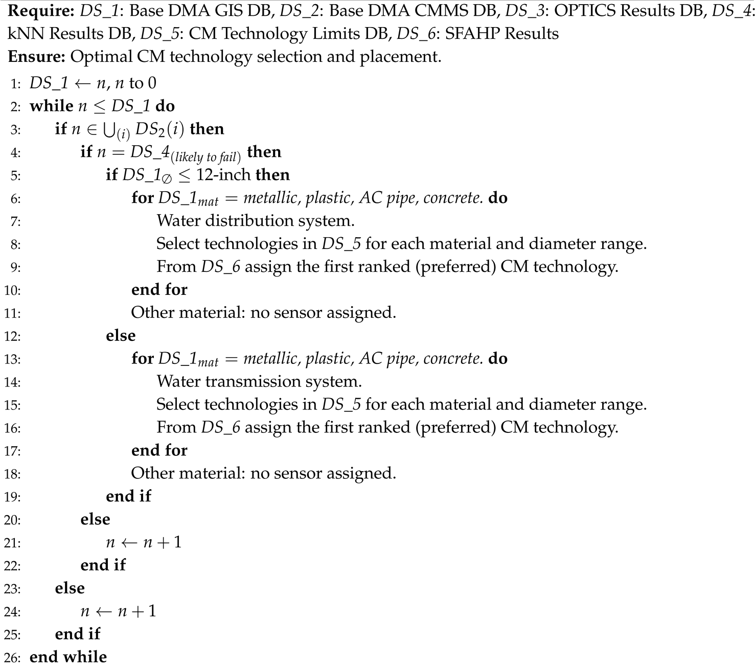
With the aforementioned sources of information, an integrative Algorithm 1 automatically determines which assets require condition monitoring and assigns the most appropriate technology. The algorithm integrates the following sources of information DS_1: base DMA GIS information (topological and physical), DS_2: base DMA CMMS information (record of failures), DS_3: results of failure prone areas with OPTICS algorithm, DS_4: results of failure prediction model with kNN, DS_5: TRL evaluation and operational limits of CM technologies, DS_6: results of the SFAHP ranking of CM technologies. Algorithm 1 works by evaluating the vulnerability of each pipe segment using two approaches, (1) its proximity to general degradation factors that occur in areas prone to failures previously indexed with an OPTICS algorithm, and (2) the likelihood of future failures as expressed from known failure factors indexed in a kNN model. If a pipe section is found to be vulnerable and likely to have failures, the pipe is classified as being part of the utility distribution or transmission system. CM technologies are selected for each qualifying pipe using the operational limits of the technology. Only the first SFAHP ranked technology is assigned.
5. Approach Implementation Through a Case Scenario
An additional objective of this study is to verify the proposed framework using synthetic network and system data. In this section, the approach described in Section 4 is applied to assign optimal CM technology using the integrative Algorithm 1, together with the results from the OPTICS and kNN models. Since this section uses a synthetic approach, the selection of technologies with TRL and SFAHP is treated as predefined rather than formulated de novo for this scenario.
Given the widespread use and reproducibility of EPANET Net3 within the body of knowledge, this section develops the scenario using preexisting Net3 system information with additional characteristics. Net3 is a well-studied system example from the EPANET manual, and is derived from the North Marin Water District (NMWD) in Novato, California [117]. It has been used to study water quality, chlorine residual, and disinfection formation modeling; however, it is also frequently used to study sensor placement [9,18,96,97]. Net3 provides information on selected topological and physical attributes, such as pipe diameter, network geometry; however, it lacks specific information on pipe material, installation dates, and history of failures. Furthermore, since hydraulic modeling with Net3 does not require consistent scaling of pipe lengths on a map, they are displayed at varying scales in EPANET. Given that the proposed OPTICS requires a consistent scale of data points and the kNN model requires input from topological and operational data, some attributes of the standard Net3 system were supplemented as shown in Table 8 for the layers related to pipes and coordinates. Other layers of Net3, such as reservoirs, tanks, and pumps, were not considered for this case.
A GIS version of Net3 was developed by exporting a shapefile using the inp2shp command of the InpTools package. The shapefiles were imported into QGIS for the addition of supplemental information indicated in Table 8. The pipe materials were assigned replicating the expansion of the system and the common pipe diameter ranges for each material. Materials such as Ductile Iron Pipe (DIP) were assigned to pipe segments located roughly at the center of the system, and materials such as High Density Polyethylene (HDPE) or Polyvinyl Chloride (PVC) assigned predominantly to the edges of the system. Pipe materials were not assigned to segments of the Net3 system directly related to tanks, reservoirs, rivers, and pumps. Figure 5 illustrates the materials and diameters for each pipe segment in Net3 as assigned for this case.
The dates when pipe segment installation occurred were assigned based on typical material use throughout time from 1920 to 2025, following a hypothetical expansion of the system. Therefore, Cast Iron Pipes (CIP) were mostly assigned installation dates from 1920 to 1950, DIP segments were assigned installation dates from 1950 to 2000, PVC and Molecularly Oriented PVC (PVCO) were assigned installation dates from 1980 to 2025, and Concrete Pressure Pipes (CPP) were assigned installation dates from 1920 to 2025. The installation date assignments also followed a hypothetical system expansion as shown in Figure 6. The extracted length of the linestrings was extracted from the map geometry and used as the pipe length attribute in lieu of the standard Net3 length, which does not coincide with the map scale.
A layer containing polygons that encircled all the pipe segments was developed to locate the system pipe failures. These pipe failures were randomly generated using the QGIS random point generator tool for polygons. The number of points that represent pipe failures was determined based on the average number of failures per 100 km a year in North America, which as reported by Barfuss [1] is equal to 7.7 breaks/100 km-yr. Each resulting failure point was assigned to the nearest pipe in the Net3 system in QGIS.
Information on the analytic geometry of each pipe failure point and pipe segment was extracted from QGIS and imported into R to run the OPTICS algorithm using the dbscan package by Hahsler et al. [118]. Since for this approach, the aim of OPTICS clustering is to develop a new data feature that describes the proximity to failure clusters which represent areas where various deterioration factors cause general degradation of pipe materials, and given that this new feature is employed in the kNN model; the dataset for OPTICS was partitioned. The incident dates were taken to partition the data into approximately 70% for model training and 30% for testing. Because the dataset for pipe failures (DS_2) included incident dates from this approach data of pipe failures from 1984 to 2024, a training set from 1985 to 2012 was created and used for clustering. The OPTICS MinPts chosen were 5 and the resulting reachability and clustering plots are shown in Figure 7.
The minimum Euclidean distance of each pipe segment centroid () from any cluster hull centroid () was calculated using Eq. 1. Then, for each pipe segment centroid () in DS_1, is compared to the maximum , where () is a dummy variable representing all pipe segments in the dataset. When calculating , or the Cluster Distance Factor (CDF), with Eq. 2, the measure is inverted so that higher values correspond to pipe segments closer to cluster hull centroids. The resulting -values for each pipe segment were aggregated into DS_1 as an independent variable of the kNN model.
The kNN model was developed by dividing the pipe failure rates dataset (DS_2) into approximately 70% for training and 30% for testing based on the failure incident date criteria. Since failures for this case were recorded from 1985 to 2024, the training dataset included pipe segments with and without a history of failures from 1985 to 2012. Likewise, the test data set included pipe segments and their failure history from 2013 to 2024. As the kNN dependent variable, the model used a true/false categorical feature indicating whether each pipe segment has a history of failures. For independent variables, the kNN model calculates a mixed multidimensional Euclidean distance of normalized features including the CDF, total number of failures, asset age, pipe material, and pipe size. A summary of the parameters used to tune the ML techniques for determining the optimal position of CM technology is included in Table 9.
The performance measures of the predicting kNN model include accuracy, sensitivity, specificity, precision, and negative predictive value. These measures are calculated per Eqs. 3, to 7, where is True Positive, is True Negative, is False Positive, and is False Negative. The performance outcome of the actual and predicted results from the developed kNN model is summarized with the confusion matrix shown in Figure 8. As observed in the resulting performance measures (Table 10), the model particularly excels in appropriately predicting which pipe segments will not have failures.
The results of the OPTICS-kNN model provide a clear identification of the pipe segments to monitor to prevent approximately 95.7% of pipe failures for a period of 11 years. Since there are 121 pipe segments in the Net3 shapefile and 31 of them were identified for monitoring by the kNN model, approximately 25% of the pipe segments require selection and deployment of CM technology. As shown in Figure 9, the pipes that require monitoring are of various materials, sizes, and lengths. Based on these characteristics, the results of a TRL evaluation, and the SFAHP ranking, an optimal CM technology can be selected. Evident TRL 9 technologies such as permanent surface mounted VAM (noise logging) sensors can be strategically deployed for metallic pipe segments such as the ones depicted on the inset map in Figure 9.
In real-world systems, an SFAHP ranking of technologies provides a preferable set of CM technologies according to factors such as cost, scalability, and wireless connectivity, among others. Suppose that the pipe segments to be monitored are the ones selected in the results of the kNN model shown in Figure 9, and that permanent VAM noise logger technology is ranked with first preference by SFAHP, Algorithm 1 works by evaluating each pipe segment in the system, filtering the segments likely to fail, determining which corresponds to the distribution and transmission systems, and assigning the permanent VAM noise logger technology according to its operational limits and the characteristics of the pipe segment (mainly material and diameter).
6. Discussion
Previous studies offer only partial solutions to the challenge of optimal selection and placement of CM technology that considers operational conditions, maintenance history, technological capabilities, failure patterns, and the needs of water utilities. Often, published research focuses on selecting or placing technologies and does not address multiple factors with minimal data sources. Typically, addressing this diverse challenge requires a vast amount of data, including soil type, groundwater levels, depths of cover, hydraulic flow, system pressures, and additional site-specific parameters. Furthermore, these methods often require extensive post-processing activities to clean, integrate, and analyze patterns in various datasets.
In contrast, the framework and components introduced in this paper address the challenge of a streamlined approach using minimal network data commonly available at most water utilities. Through the RERAV-based approach and an integrative Algorithm 1, an optimal solution can be derived using standard water system information and standard data handling. By integrating data from CM technology performance attributes with topological, physical, and historical network data, the framework provides the following benefits.
- Suitability for analyzing entire water system networks at once, or by DMA, pipe size ranges (distribution or transmission systems), neighborhood, and so forth.
- Ability to reevaluate technology readiness and eventually include emerging methods that currently have the potential to revolutionize CM of underground infrastructure (e.g., QST and SSM).
- Adaptability to meet the needs and goals of different types and sizes of water utilities by systematically ranking CM methods based on their functionality and varying operational environments.
- Possibility of providing more or less importance to technology costs, wireless connectivity, scalability, power requirements, installation complexity, and additional criteria of importance to utilities.
- Applicability to most water utilities due to its lower special data requirements. The approach utilizes data features typically employed for regular water audits and loss control studies.
- Ability to discern which pipelines in vulnerable areas have a higher chance of failure, thus requiring specific CM based on its physical, topological, and material characteristics.
The approach introduced in this paper is not a fully automated process, it requires human intervention to define some criteria, especially those related to the SFAHP ranking of CM technologies. Despite the need to provide expert knowledge for decision-making, the methodology is considered to have reduced levels of complexity, since its implementation can be achieved with well-known ML algorithms and standard data sources. Furthermore, an automated solution for any water utility is not practical since utilities have their unique resource challenges, requiring case-by-case adjustments of AHP criteria to suit those particular needs.
Future research to explore applicability in real-world systems and conduct optimization methods to improve robustness by identifying noise-generating factors that can lead to unreliable results. Additionally, it is encouraged to explore the application of the introduced REVAV-based approach for the location of sensors directly on system appurtenances (e.g., hydrants and valves), which are generally the locations where CM technologies are deployed.
7. Conclusions
Although studies and industry reports suggest a modest improvement in overall water main infrastructure conditions, the deterioration of large, dispersed, and strategic water assets continues to be a cause of significant economic losses due to unforeseen failures of unsupervised assets. Addressing this issue requires methods to determine both suitable technology and precise positioning based on the conditions and performance of the system. However, current strategies traditionally rely on complex algorithms and vast amounts of data from sources often of insufficient quality or not readily available at utilities. Furthermore, current research has focused on separate analyses for the choice of sensor and optimal sensor placement, employing modeled hydraulic data while disregarding historical system performance. A successful condition monitoring program must incorporate accurate technology selection and precise technology placement, effectively detecting most early warnings of compromised strategic assets, preventing leaks and breaks, prioritizing repairs, and ultimately reducing infrastructure maintenance costs.
This study provided a comprehensive review of CA and CM technologies, along with common approaches to selecting and placing technology. To the authors’ knowledge, no previous research has proposed a CDF derived from the centroids of OPTICS cluster convex hulls as a measure to evaluate pipe segment vulnerability due to proximity to failure prone areas. Additionally, a unified approach for positioning and selecting optimal CM technology for water supply systems has not been documented in the existing body of knowledge. The demonstration of the usefulness of OPTICS, CDF, and the kNN model using minimal physical, topological and maintenance data through a synthetic benchmark (Net3) highlights the feasibility of this innovative approach. Hence, building on earlier work, this study documents an innovative approach grounded in a REVAV-based framework, that integrates structured decision-making techniques and ML algorithms. The study expands its innovative reach by introducing an integrative algorithm that uses asset management principles to automatically assign CM technology to pipelines at the highest risk of failure. Finally, due to the minimal data requirements, and standard GIS and CMMS data sources, the framework and methods presented in this article are highly adaptable to real-world systems.
Author Contributions
Conceptualization, D.C.; methodology, D.C.; formal analysis, D.C.; investigation, D.C.; writing—original draft preparation, D.C.; writing—review and editing, D.C.; visualization, D.C.; supervision, M.N. All authors have read and agreed to the published version of the manuscript.
Funding
This study was partly supported by The Water Research Foundation (WRF) project 5191 "Innovative Technologies to Improve Monitoring of Assets."
Conflicts of Interest
The authors declare no conflicts of interest.
References
- Barfuss, S.L. Water Main Break Rates in the USA and Canada: A Comprehensive Study; Technical report; Utah Water Research Laboratory, Utah State University: 2023.
- ASCE. 2021 Report Card for America’s Infrastructure; Technical report; American Society of Civil Engineers (ASCE): Reston, Virginia, USA, 2021.
- Najafi, M.; Gokhale, S.B.; Calderon, D.R.; Ma, B. Trenchless Technology: Pipeline and Utility Design, Construction, and Renewal, second ed.; McGraw Hill: New York [NY], 2022.
- Bornhofen, R. DC Water’s Journey to Gen AI. In Proceedings of the Proceedings of the Water Environment Federation. Water Environment Federation, 2024. [CrossRef]
- Culshaw, B.; Kersey, A. Fiber-Optic Sensing: A Historical Perspective. Journal of Lightwave Technology 2008, 26, 1064–1078. [CrossRef]
- Broeke, Joep van den.; Carpentier, Corina.; Moore, Colin.; Carswell, Leo.; Jonsson, J"orgen.; Sivil, David.; Rosen, Jeffrey.; Cade, Lucia.; Mofidi, Alex.; Swartz, Chris.; et al. Compendium of Sensors and Monitors and Their Use in the Global Water Industry; Water Environment Research Foundation (WERF) and IWA Publishing: 2014.
- Hunt, T.M. The Concise Encyclopaedia of Condition Monitoring: Including a Guide to 15 Condition Monitoring Techniques, 1. ed ed.; Machine & Systems Condition Monitoring Series; Coxmoor Publ Co: Chipping Norton, 2006.
- ChenLei, X.; QianSheng, F.; HongYan, Z.; JiXin, Z. Optimal Layout of Pressure Monitoring Points in Water Supply Network Based on Optics. In Proceedings of the E3S Web of Conferences, 2019.
- Yang, G.; Wang, H. Optimal Pressure Sensor Deployment for Leak Identification in Water Distribution Networks. Sensors 2023, 23, 5691. [CrossRef]
- Cuguero-Escofet, M.A.; Puig, V.; Quevedo, J.; Blesa, J. Optimal Pressure Sensor Placement for Leak Localisation Using a Relaxed Isolation Index: Application to the Barcelona Water Network. IFAC-PapersOnLine 2015, 48, 1108–1113. [CrossRef]
- Jun, S.; Kwon, H.J. The Optimum Monitoring Location of Pressure in Water Distribution System. Water 2019, 11, 307. [CrossRef]
- Saldarriaga, J.; Salcedo, C.A. Determination of Optimal Location and Settings of Pressure Reducing Valves in Water Distribution Networks for Minimizing Water Losses. Procedia Engineering 2015, 119, 973–983. [CrossRef]
- Ferreira, B.; Antunes, A.; Carriço, N.; Covas, D. NSGA-II Parameterization for the Optimal Pressure Sensor Location in Water Distribution Networks. Urban Water Journal 2023, 20, 738–750. [CrossRef]
- Nejjari, F.; Sarrate, R.; Blesa, J. Optimal Pressure Sensor Placement in Water Distribution Networks Minimizing Leak Location Uncertainty. Procedia Engineering 2015, 119, 953–962. [CrossRef]
- Soroush, F.; Abedini, M.J. Optimal Selection of Number and Location of Pressure Sensors in Water Distribution Systems Using Geostatistical Tools Coupled with Genetic Algorithm. Journal of Hydroinformatics 2019, 21, 1030–1047. [CrossRef]
- Santos-Ruiz, I.; Lopez-Estrada, F.R.; Puig, V.; Valencia-Palomo, G.; Hernandez, H.R. Pressure Sensor Placement for Leak Localization in Water Distribution Networks Using Information Theory. Sensors 2022, 22, 443. [CrossRef]
- Chang, N.B.; Prapinpongsanone, N.; Ernest, A. Optimal Sensor Deployment in a Large-Scale Complex Drinking Water Network: Comparisons between a Rule-Based Decision Support System and Optimization Models. Computers & Chemical Engineering 2012, 43, 191–199. [CrossRef]
- Du, K.; Yu, J.; Zheng, F.; Xu, W.; Savic, D.; Kapelan, Z. A Robust Multi-Objective Pressure Sensor Placement Method for Burst Detection in Water Distribution Systems. Water Resources Research 2024, 60, e2024WR037258. [CrossRef]
- Lau, H.; Dwight, R. A Fuzzy-Based Decision Support Model for Engineering Asset Condition Monitoring – A Case Study of Examination of Water Pipelines. Expert Systems with Applications 2011, 38, 13342–13350. [CrossRef]
- Tscheikner-Gratl, F.; Egger, P.; Rauch, W.; Kleidorfer, M. Comparison of Multi-Criteria Decision Support Methods for Integrated Rehabilitation Prioritization. Water 2017, 9, 68. [CrossRef]
- Zhang, W.; Lai, T.; Li, Y. Risk Assessment of Water Supply Network Operation Based on ANP-Fuzzy Comprehensive Evaluation Method. Journal of Pipeline Systems Engineering and Practice 2022, 13, 04021068. [CrossRef]
- Allen, M.; Preis, A.; Iqbal, M.; Whittle, A.J. Water Distribution System Monitoring and Decision Support Using a Wireless Sensor Network. In Proceedings of the 2013 14th ACIS International Conference on Software Engineering, Artificial Intelligence, Networking and Parallel/Distributed Computing, Honolulu, HI, USA, 2013; pp. 641–646. [CrossRef]
- Davis, P.; Sullivan, E.; Marlow, D.; Marney, D. A Selection Framework for Infrastructure Condition Monitoring Technologies in Water and Wastewater Networks. Expert Systems with Applications 2013, 40, 1947–1958. [CrossRef]
- Yazdekhasti, S.; Piratla, K.R.; Matthews, J.C.; Khan, A.; Atamturktur, S. Optimal Selection of Acoustic Leak Detection Techniques for Water Pipelines Using Multi-Criteria Decision Analysis. Management of Environmental Quality: An International Journal 2018, 29, 255–277. [CrossRef]
- Reed, C.; Robinson, A.J.; Smart, D. Techniques for Monitoring Structural Behaviour of Pipeline Systems; Awwa Research Foundation and American Water Works Association: Denver, CO, 2004.
- Hangan, A.; Chiru, C.G.; Arsene, D.; Czako, Z.; Lisman, D.F.; Mocanu, M.; Pahontu, B.; Predescu, A.; Sebestyen, G. Advanced Techniques for Monitoring and Management of Urban Water Infrastructures—An Overview. Water 2022, 14, 2174. [CrossRef]
- ASCE. Water Pipeline Condition Assessment; ASCE Manuals and Reports on Engineering Practice No. 134, American Society of Civil Engineers (ASCE): Reston, VA, 2017. [CrossRef]
- AWWA. Manual M77 Condition Assessment of Water Mains; Manual of Water Supply Practices; American Water Works Association: Denver, CO, 2019.
- Marshall, D.H.; Worthington, W. Increasing the Reliability of Concrete Pressure Pipe. In Proceedings of the Trenchless Pipeline Projects Practical Applications, Boston, Massachusetts, USA, 1997; pp. 273–282. [CrossRef]
- NASSCO. Pipeline Assessment and Certification Program (PACP™) Reference Manual, Version 8, version 8 ed.; NASSCO Inc.: Frederick, Maryland, USA., 2023.
- Liu, Z.; Kleiner, Y. State of the Art Review of Inspection Technologies for Condition Assessment of Water Pipes. Measurement 2013, 46, 1–15. [CrossRef]
- Farrar, C.R.; Worden, K. An Introduction to Structural Health Monitoring. Philosophical Transactions of the Royal Society A: Mathematical, Physical and Engineering Sciences 2007, 365, 303–315. [CrossRef]
- Metje, N.; Chapman, D.; Walton, R.; Sadeghioon, A.; Ward, M. Real Time Condition Monitoring of Buried Water Pipes. Tunnelling and Underground Space Technology 2012, 28, 315–320. [CrossRef]
- WSSC Water. WSSC Water Strategic Plan Fiscal Year 2025-2027; Technical report; Washington Suburban Sanitary Commission (WSSC): 2024.
- US EPA. Water and Wastewater Systems Sector-Specific Plan, 2015.
- Liu, Z.; Kleiner, Y. State-of-the-Art Review of Technologies for Pipe Structural Health Monitoring. IEEE Sensors Journal 2012, 12, 1987–1992. [CrossRef]
- Latif, J.; Shakir, M.Z.; Edwards, N.; Jaszczykowski, M.; Ramzan, N.; Edwards, V. Review on Condition Monitoring Techniques for Water Pipelines. Measurement 2022, 193, 110895. [CrossRef]
- EPA. Innovation and Research for Water Infrastructure for the 21st Century Research Plan. Technical Report EPA/600/X-09/003, U.S. Environmental Protection Agency (EPA), 2007.
- Hertlein, B.H. Stress Wave Testing of Concrete: A 25-Year Review and a Peek into the Future. Construction and Building Materials 2013, 38, 1240–1245. [CrossRef]
- Ali, H.; Choi, J.h. A Review of Underground Pipeline Leakage and Sinkhole Monitoring Methods Based on Wireless Sensor Networking. Sustainability 2019, 11, 4007. [CrossRef]
- Obeid, A.; Karray, F.; Jmal, W.; Abid, M.; Qasim, S.M.; Bensaleh, M. Toward Realisation of Wireless Sensor Network Based Water Pipeline Monitoring Systems: A Comprehensive Review of Techniques and Platforms. IET Science Measurement ? Technology 2016, 10. [CrossRef]
- Gupta, A.; Kulat, K.D. A Selective Literature Review on Leak Management Techniques for Water Distribution System. Water Resources Management 2018, 32, 3247–3269. [CrossRef]
- Stanczyk, J.; Burszta, E. Development of Methods for Diagnosing the Operating Conditions of Water Supply Networks over the Last Two Decades. Water 2022, 14, 786. [CrossRef]
- Li, R.; Huang, H.; Xin, K.; Tao, T. A Review of Methods for Burst/Leakage Detection and Location in Water Distribution Systems. Water Supply 2015, 15, 429–441. [CrossRef]
- Liu, Z.; Kleiner, Y. Computational Intelligence for Urban Infrastructure Condition Assessment: Water Transmission and Distribution Systems. IEEE Sensors Journal 2014, 14, 4122–4133. [CrossRef]
- Wang, Y.Y. Management of Ground Movement Hazards for Pipelines. Technical Report CRES-2012-M03-01, Interstate Natural Gas Association of America (INGAA), 2017.
- Rizzo, P. Water and Wastewater Pipe Nondestructive Evaluation and Health Monitoring: A Review. Advances in Civil Engineering 2010, 2010, 818597. [CrossRef]
- Ojdrovic, R.; Nardini, P.D.; Bracken, M.; Marciszewski, J. Evaluation of Acoustic Wave Based PCCP Stiffness Testing Results. In Proceedings of the ASCE UESI Pipelines 2015. American Society of Civil Engineers, 2015, pp. 1150–1159. [CrossRef]
- Williams, A.F.; Peterson, K.A.; Nardini, P.D.; Ojdrovic, R.P. Condition Assessment and Repair Prioritization of a Large Diameter Pipeline System. In Proceedings of the ASCE UESI Pipelines 2019. American Society of Civil Engineers, 2019, pp. 95–104. [CrossRef]
- Kumar, S.S.; Abraham, D.M.; Behbahani, S.S.; Matthews, J.C.; Iseley, T. Comparison of Technologies for Condition Assessment of Small-Diameter Ductile Iron Water Pipes. Journal of Pipeline Systems Engineering and Practice 2020, 11, 04020039. [CrossRef]
- Lu, H.; Xu, Z.D.; Iseley, T.; Peng, H.; Fu, L. Pipeline Inspection and Health Monitoring Technology: The Key to Integrity Management; Springer Nature Singapore: Singapore, 2023. [CrossRef]
- Bykerk, L.; Valls Miro, J. Detection of Water Leaks in Suburban Distribution Mains with Lift and Shift Vibro-Acoustic Sensors. Vibration 2022, 5, 370–382. [CrossRef]
- Yang, L. Techniques for Corrosion Monitoring; Woodhead Publishing, 2020.
- Fessler, R. Pipeline Corrosion. Technical report, U.S. Department of Transportation, Pipeline and Hazardous Materials Safety Administration, 2008.
- Bohannon, T.; Boozer, C. From Satellite to Snout: How Central Arkansas Water Uses High- Tech and Low-Tech to Attack Nonrevenue Water. In Proceedings of the 2021 Weftec. Water Environment Federation, 2021.
- Leung, C.K.Y.; Wan, K.T.; Inaudi, D.; Bao, X.; Habel, W.; Zhou, Z.; Ou, J.; Ghandehari, M.; Wu, H.C.; Imai, M. Review: Optical Fiber Sensors for Civil Engineering Applications. Materials and Structures 2015, 48, 871–906. [CrossRef]
- Barrias, A.; Casas, J.; Villalba, S. A Review of Distributed Optical Fiber Sensors for Civil Engineering Applications. Sensors 2016, 16, 748. [CrossRef]
- Krohn, D.A.; MacDougall, T.; Mendez, A. Fiber Optic Sensors: Fundamentals and Applications, 4. ed ed.; Number 247 in SPIE PM, SPIE Press: Bellingham, Wash, 2014.
- Ravet, F.; Bracken, M.; Dutoit, D.; Nikles, M.; Sa, O.; Ch, R.B. Extended Distance Fiber Optic Monitoring for Pipeline Leak and Ground Movement Detection. In Proceedings of the ASCE Pipelines 2009, 2009. [CrossRef]
- Braga, A.M.B.; Valente, L.C.G.; Llerena, R.W.A.; Regazzi, R.D. Optical Fiber Sensing Technology in the Pipeline Industry. In Proceedings of the Rio Pipeline 2003 Conference & Exposition, Rio de Janeiro, 2003.
- Dunbar, J.; Galan-Comas, G.; Walshire, L.; Wahl, R.; Yule, D.; Corcoran, M.; Bufkin, A.; Llopis, J. Remote Sensing and Monitoring of Earthen Flood-Control Structures. Technical report, Geotechnical and Structures Laboratory (U.S.), 2017. [CrossRef]
- Helz, R. Monitoring Ground Deformation from Space, 2005.
- Robles, D.; Castillo, E. Case of Geotechnical Instrumentation of Pipelines in Unstable Zones: Real Time Readings and Its Development in Uncommunicated Zones. In Proceedings of the Proceedings of the ASME International Pipeline Geotechnical Conference, Lima, Peru, 2017.
- Edemsky, D.; Popov, A.; Prokopovich, I.; Garbatsevich, V. Airborne Ground Penetrating Radar, Field Test. Remote Sensing 2021, 13, 667. [CrossRef]
- Halimshah, N.N.; Yusup, A.; Mat Amin, Z.; Ghazalli, M.D. Visual Inspection of Water Leakage from Ground Penetrating Radar Radargram. ISPRS Annals of the Photogrammetry, Remote Sensing and Spatial Information Sciences 2015, II-2/W2, 191–198. [CrossRef]
- Crocco, L.; Soldovieri, F.; Millington, T.; Cassidy, N.J. Bistatic Topographic GRP Imaging for Incipient Pipeline Leakage Evaluation. Progress In Electromagnetics Research 2010, 101, 307–321. [CrossRef]
- Aslam, H.; Mortula, M.M.; Yehia, S.; Ali, T.; Kaur, M. Evaluation of the Factors Impacting the Water Pipe Leak Detection Ability of GPR, Infrared Cameras, and Spectrometers under Controlled Conditions. Applied Sciences 2022, 12, 1683. [CrossRef]
- Fahmy, M.; Moselhi, O. Automated Detection and Location of Leaks in Water Mains Using Infrared Photography. Journal of Performance of Constructed Facilities 2010, 24, 242–248. [CrossRef]
- Allouche, E.; Sari, M.A.; Alfaqih, L.; Oppenheimer, J.; Ibikunle, O.; Snow, J.R.; Jacangelo, J.G. Innovative Technologies to Effectively Manage Deteriorating Infrastructure. Technical Report WRF 4717, The Water Research Foundation, Alexandria, VA, USA., 2020.
- Hawari, A.; Khader, M.; Hirzallah, W.; Zayed, T.; Moselhi, O. Integrated Sensing Technologies for Detection and Location of Leaks in Water Distribution Networks. Water Supply 2017, 17, 1589–1601. [CrossRef]
- Karbhari, V.M.; Ansari, F. Structural Health Monitoring of Civil Infrastructure Systems; Woodhead Publishing Limited, 2009. [CrossRef]
- Hadji, A.; Flazi, S.; Bouzid, M.A. Novel Electrical Technique for Detecting Water Leaks in Buried Plastic Water Distribution Pipes. Journal of Pipeline Systems Engineering and Practice 2022, 13, 04022043. [CrossRef]
- Adedeji, K.B.; Hamam, Y.; Abe, B.T.; Abu-Mahfouz, A.M. Towards Achieving a Reliable Leakage Detection and Localization Algorithm for Application in Water Piping Networks: An Overview. IEEE Access 2017, 5, 20272–20285. [CrossRef]
- Datta, S.; Sarkar, S. A Review on Different Pipeline Fault Detection Methods. Journal of Loss Prevention in the Process Industries 2016, 41, 97–106. [CrossRef]
- Chapman, J.; Seskir, Z.C. Quantum Sensing Technologies and Smart Cities: Opportunities and Challenges. In Proceedings of the Proceedings of the 10th IEEE International Smart Cities Conference, Pattaya City, Thailand, 2024.
- Kantsepolsky, B.; Aviv, I. Sensors in Civil Engineering: From Existing Gaps to Quantum Opportunities. Smart Cities 2024, 7, 277–301. [CrossRef]
- Kantsepolsky, B.; Aviv, I.; Weitzfeld, R.; Bordo, E. Exploring Quantum Sensing Potential for Systems Applications. IEEE Access 2023, 11, 31569–31582. [CrossRef]
- Almazyad, A.S.; Seddiq, Y.M.; Alotaibi, A.M.; Al-Nasheri, A.Y.; BenSaleh, M.S.; Obeid, A.M.; Qasim, S.M. A Proposed Scalable Design and Simulation of Wireless Sensor Network-Based Long-Distance Water Pipeline Leakage Monitoring System. Sensors 2014, 14, 3557–3577. [CrossRef]
- Weiming, W.; Jian, W.; Kun, T. Development of a Chipless RFID Water Leakage Detecting Sensor Using Defected Ground Structure. In Proceedings of the 2022 International Applied Computational Electromagnetics Society Symposium (ACES-China), 2022, pp. 1–2. [CrossRef]
- Khomenko, A.; Koricho, E.G.; Haq, M.; Cloud, G.L. Bolt Tension Monitoring with Reusable Fiber Bragg-grating Sensors. The Journal of Strain Analysis for Engineering Design 2016, 51, 101–108. [CrossRef]
- Thompson, L.D.; Westermo, B.D.; Crum, D.B.; Law, W.; Trombi, R.; Waldbusser, R. Smart Structural Fasteners for the Aircraft and Construction Industries. In Proceedings of the 1999 Symposium on Smart Structures and Materials; Wereley, N.M., Ed., Newport Beach, CA, 1999; pp. 143–152. [CrossRef]
- Kim, Y.; Jung, H.; Ryou, J.; Choi, J. A Basic Experimental Study on Analysis of Leak Signal and Monitoring Method for Water Supply Pipe. Applied Sciences 2021, 11, 2097. [CrossRef]
- Han, B.; Ding, S.; Yu, X. Intrinsic Self-Sensing Concrete and Structures: A Review. Measurement 2015, 59, 110–128. [CrossRef]
- Perry, G.; Goldfeld, Y. Smart Self-Sensory TRC Pipes—Proof of Concept. Smart Materials and Structures 2022, 31, 055011. [CrossRef]
- Lee, P.J.; Lambert, M.F.; Simpson, A.R.; V’itkovsky, J.P.; Misiunas, D. Leak Location in Single Pipelines Using Transient Reflections. Australasian Journal of Water Resources 2007, 11, 53–65. [CrossRef]
- Jin, S.; Saparia, B.; Norton, J.; Wood, B.; Abdallah, A.; McClinton, T.; Burchi, J.; Radtke, L. Monitoring of Pressure Transients in Great Lakes Water Authority Water Transmission System. Journal of Water Management Modeling 2022. [CrossRef]
- Surucu, O.; Gadsden, S.A.; Yawney, J. Condition Monitoring Using Machine Learning: A Review of Theory, Applications, and Recent Advances. Expert Systems with Applications 2023, 221, 119738. [CrossRef]
- Abdelmageed, S.; Tariq, S.; Boadu, V.; Zayed, T. Criteria-Based Critical Review of Artificial Intelligence Applications in Water-Leak Management. Environmental Reviews 2022, 30, 280–297. [CrossRef]
- Azimi, M.; Eslamlou, A.; Pekcan, G. Data-Driven Structural Health Monitoring and Damage Detection through Deep Learning: State-of-the-Art Review. Sensors 2020, 20, 2778. [CrossRef]
- Yazdekhasti, S.; Vladeanu, G.; Daly, C. Evaluation of Artificial Intelligence Tool Performance for Predicting Water Pipe Failures. In Proceedings of the Pipelines 2020, San Antonio, Texas (Conference Held Virtually), 2020; pp. 203–211. [CrossRef]
- Housner, G.W.; Bergman, L.A.; Caughey, T.K.; Chassiakos, A.G.; Claus, R.O.; Masri, S.F.; Skelton, R.E.; Soong, T.T.; Spencer, B.F.; Yao, J.T.P. Structural Control: Past, Present, and Future. Journal of Engineering Mechanics 1997, 123, 897–971. [CrossRef]
- La Rose, K.; Sagiannos, V.; Hebner, J. A Comprehensive Condition Assessment of a High Risk Coastal Force Main: Comox Valley Regional District Case Study. In Proceedings of the Pipelines 2018, Toronto, Ontario, Canada, 2018; pp. 239–248. [CrossRef]
- Sela, L.; Amin, S. Robust Sensor Placement for Pipeline Monitoring: Mixed Integer and Greedy Optimization. Advanced Engineering Informatics 2018, 36, 55–63. [CrossRef]
- Calderon, D.; Bavilinezhad, S.; Hamidzadeh, P.; Rajaie, E.; Najafi, M. Trenchless Technology Research Needs: Results and Conclusions from an Industry Research Symposium. In Proceedings of the 2024 No-Dig Show, Providence, RI, 2024.
- Holley, M.; Diaz, R.; Giovanniello, M. Acoustic Monitoring of Prestressed Concrete Cylinder Pipe: A Case History. In Proceedings of the ASCE Pipelines 2001. American Society of Civil Engineers, 2001, pp. 1–9. [CrossRef]
- Zhao, M.; Zhang, C.; Liu, H.; Fu, G.; Wang, Y. Optimal Sensor Placement for Pipe Burst Detection in Water Distribution Systems Using Cost–Benefit Analysis. Journal of Hydroinformatics 2020, 22, 606–618. [CrossRef]
- Zecchin, A.C.; Do, N.; Gong, J.; Leonard, M.; Lambert, M.F.; Stephens, M.L. Optimal Pipe Network Sensor Layout Design for Hydraulic Transient Event Detection and Localization. Journal of Water Resources Planning and Management 2022, 148, 04022041. [CrossRef]
- Hu, Z.; Chen, W.; Chen, B.; Tan, D.; Zhang, Y.; Shen, D. Robust Hierarchical Sensor Optimization Placement Method for Leak Detection in Water Distribution System. Water Resources Management 2021, 35, 3995–4008. [CrossRef]
- Xie, X.; Zhou, Q.; Hou, D.; Zhang, H. Compressed Sensing Based Optimal Sensor Placement for Leak Localization in Water Distribution Networks. Journal of Hydroinformatics 2018, 20, 1286–1295. [CrossRef]
- Rayaroth, R.; G, S. Random Bagging Classifier and Shuffled Frog Leaping Based Optimal Sensor Placement for Leakage Detection in WDS. Water Resources Management 2019, 33, 3111–3125. [CrossRef]
- Menapace, A.; Zanfei, A.; Herrera, M.; Brentan, B. Graph Neural Networks for Sensor Placement: A Proof of Concept towards a Digital Twin of Water Distribution Systems. Water 2024, 16, 1835. [CrossRef]
- Zarghamee, M.S.; Ojdrovic, R.P.; Nardini, P.D. Prestressed Concrete Cylinder Pipe Condition Assessment—What Works, What Doesn’t, What’s Next 2012. pp. 182–194. [CrossRef]
- Ankerst, M.; Breunig, M.M.; Kriegel, H.P.; Sander, J. OPTICS: ordering points to identify the clustering structure. ACM SIGMOD Record 1999, 28, 49–60. [CrossRef]
- Metz, M. GRASS GIS 8.4.2dev Reference Manual. https://grass.osgeo.org/grass-stable/manuals/v.cluster.html, 2024.
- Huang, C.C. Detect Spatial-Temporal Point Clusters by Incorporating Time into Density-based Clustering. https://www.esri.com/arcgis-blog/products/arcgis-pro/analytics/detect-spatial-temporal-point-clusters-by-incorporating-time-into-density-based-clustering/, 2021.
- Calderon, D.; Najafi, M. Water Asset Condition Monitoring Classification: Investigating the Use of Machine Learning. In Proceedings of the International No-Dig 2023, Mexico City, Mexico, 2023.
- Yussif, A.M.; Sadeghi, H.; Zayed, T. Application of Machine Learning for Leak Localization in Water Supply Networks. Buildings 2023, 13, 849. [CrossRef]
- IBM. What Is the K-Nearest Neighbors Algorithm? | IBM. https://www.ibm.com/think/topics/knn, 2021.
- Zhang, S.; Li, X.; Zong, M.; Zhu, X.; Cheng, D. Learning k for kNN Classification. ACM Transactions on Intelligent Systems and Technology 2017, 8, 1–19. [CrossRef]
- Heder, M. From NASA to EU: The Evolution of the TRL Scale in Public Sector Innovation. The Innovation Journal 2017.
- NASA., Ed. NASA Systems Engineering Handbook; Number SP-2016-6105 Rev2, National Aeronautics and Space Administration (NASA): Washington, D.C, 2017.
- PRCI. Technology Readiness Levels, Pipeline Research Council International (PRCI). https://www.prci.org, 2017.
- Deshmukh-Towery, N.; Machek, E.C.; Thomas, A. Technology Readiness Level Guidebook. Technical Report FHWA-HRT-17-047, Federal Highway Administration (FHWA), US Department of Transportation (USDOT), McLean, Virginia, USA., 2017.
- Abdelkader, E.M.; Zayed, T.; Elshaboury, N. A Novel Hybrid Fuzzy Analytical Hierarchy Process–Game Theory Model for Prioritizing Factors Affecting the Deterioration of Water Pipelines. Applied Water Science 2024, 14, 265. [CrossRef]
- Kutlu Gundogdu, F.; Kahraman, C. A Novel Spherical Fuzzy Analytic Hierarchy Process and Its Renewable Energy Application. Soft Computing 2020, 24, 4607–4621. [CrossRef]
- Dogan, O. Process Mining Technology Selection with Spherical Fuzzy AHP and Sensitivity Analysis. Expert Systems with Applications 2021, 178, 114999. [CrossRef]
- Rossman, L. EPANET Net3 System Description; Software Manual Examples 2, University of Kentucky Libraries, 2016.
- Hahsler, M.; Piekenbrock, M.; Doran, D. dbscan: Fast Density-Based Clustering with R. Journal of Statistical Software 2019, 91, 1–30. [CrossRef]
Figure 1.
Multi-Dimensional Classification of CA and CM Technologies for Water Assets.
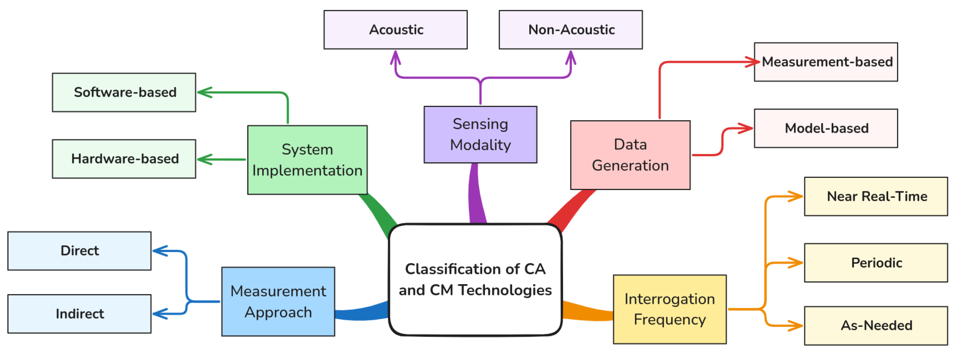
Figure 2.
Process Diagram for a RERAV-based Selection and Placement of CM Technology.
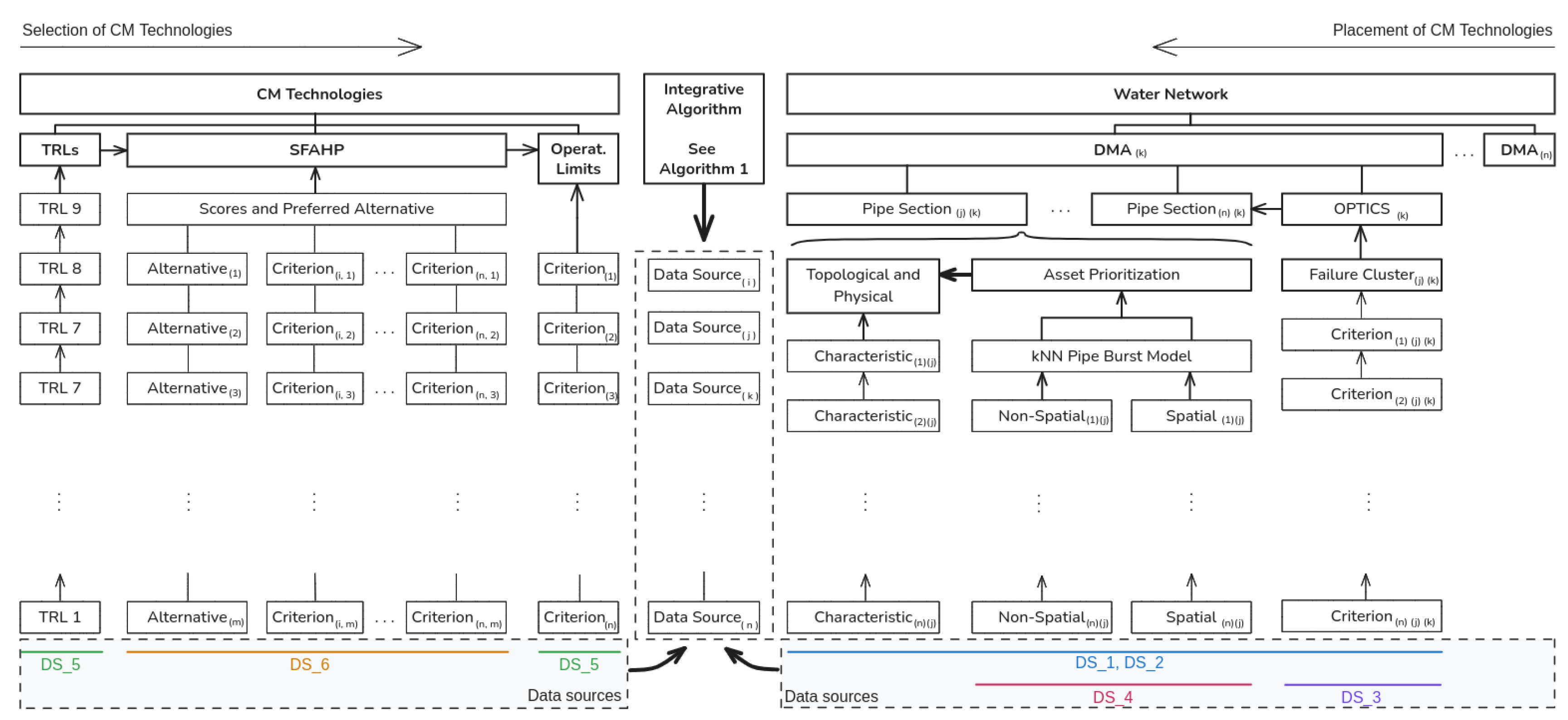
Figure 3.
TRL System for Evaluating CM Technologies.
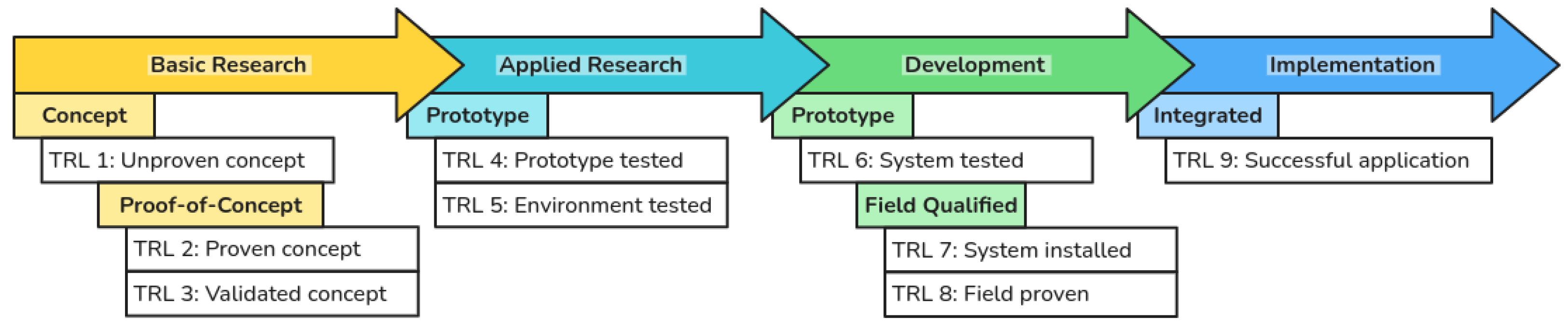
Figure 4.
SFAHP Hierarchical Structure.
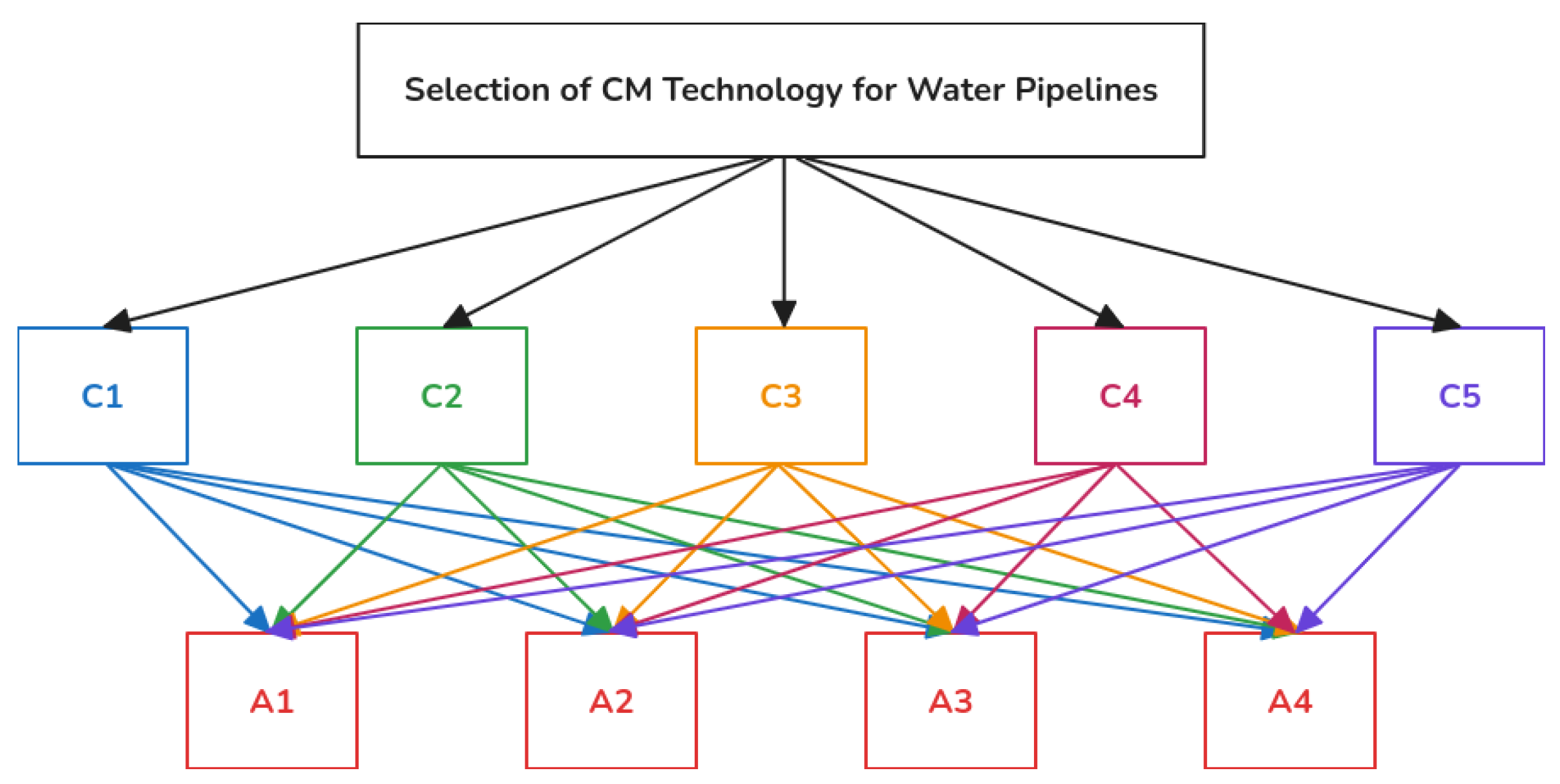
Figure 5.
Pipe Segment Size and Materials for the Modified Version of Net3.
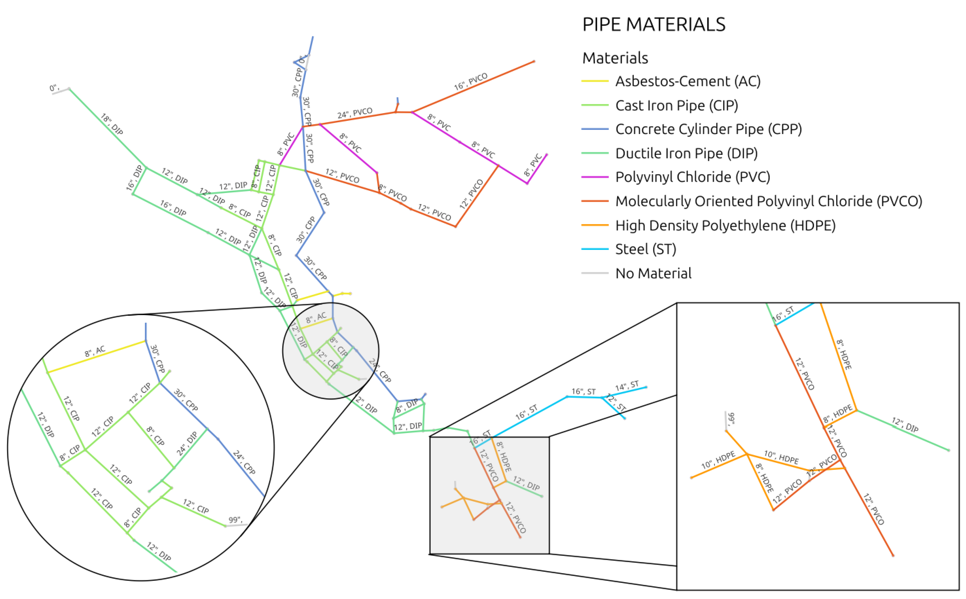
Figure 6.
Net3 Hypothetical System Expansion Used for the Case Scenario.
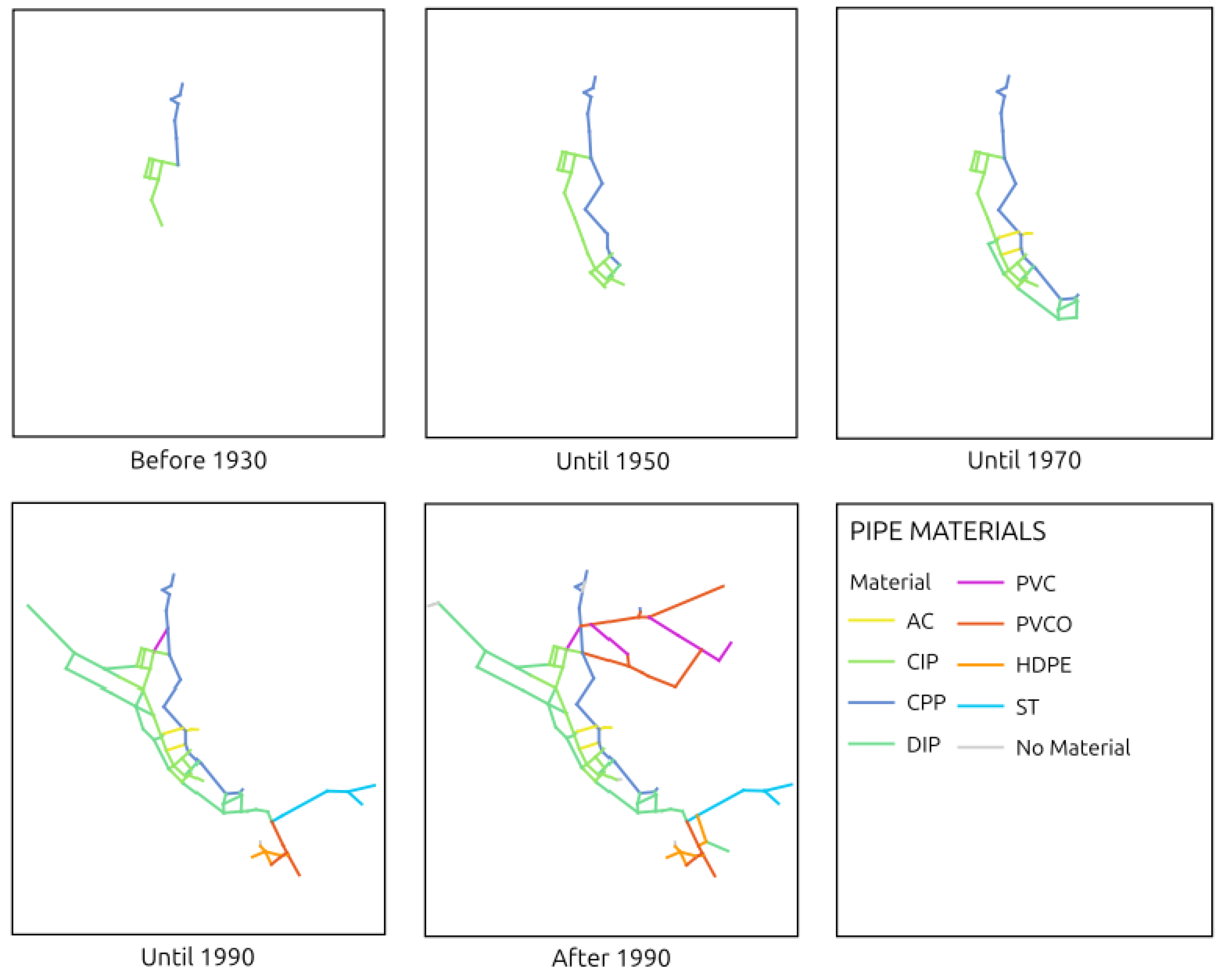
Figure 7.
Results of OPTICS Clustering for System Failures with eps_cl = 3.
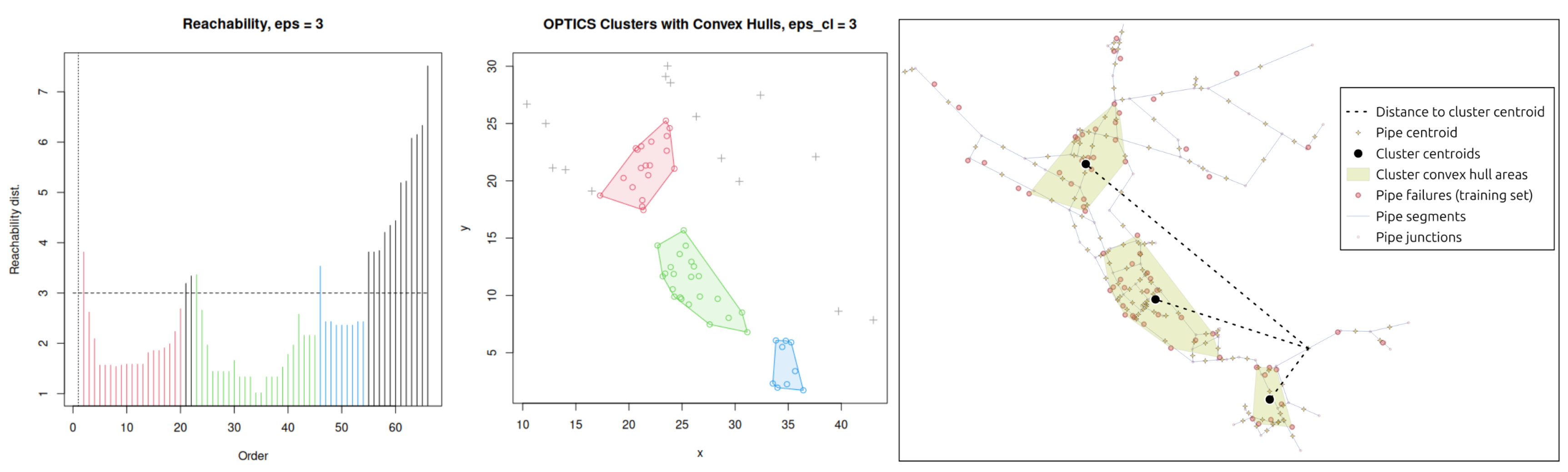
Figure 8.
Resulting Confusion Matrix for kNN Model
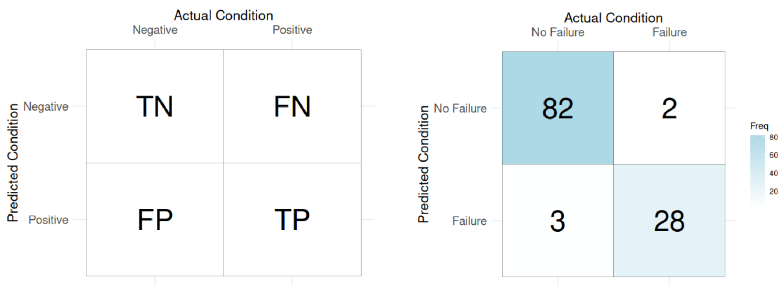
Figure 9.
Predicted Pipes to Monitor Based on the OPTICS-kNN Model
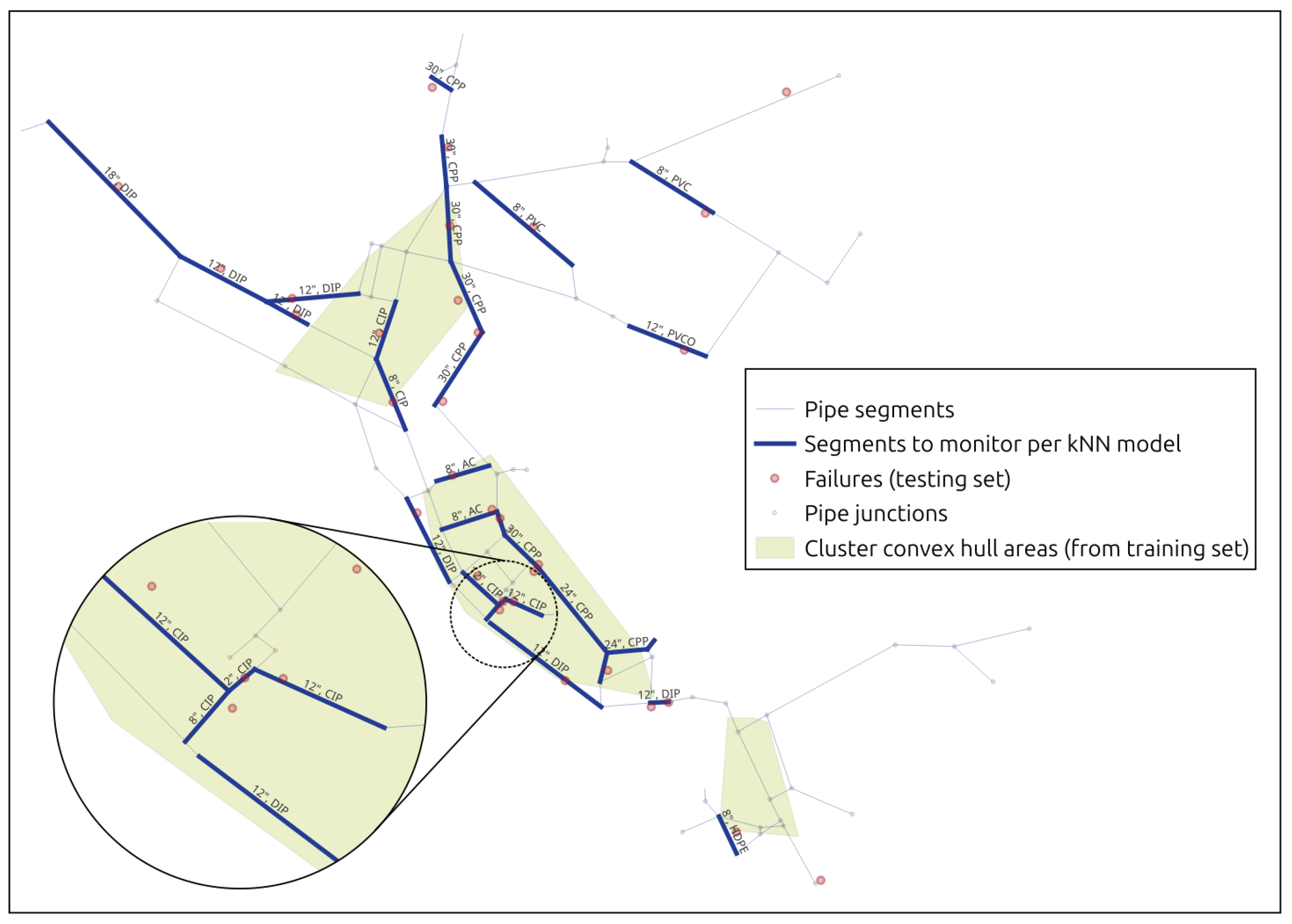

Table 1.
List of Acronyms and Abbreviations.
| Acronyms | Description | Acronyms | Description |
|---|---|---|---|
| AC | Asbestos-Cement | MFL | Magnetic Flux Leakage |
| AET | Acoustic Emission Testing | MinPts | Minimum domain points to form dense regions |
| AHP | Analytic Hierarchy Process | ML | Machine Learning |
| BEM | Broadband Electromagnetic | NDE | Non-Destructive Evaluation |
| CA | Condition Assessment | NDT | Non-Destructive Testing |
| CAPEX | Capital Expenses | NGSA-II | Non-dominated Sorting Genetic Algorithm II |
| CBA | Cost-Benefit Analysis | NPW | Negative Pressure Waves |
| CCM | Chemical Composition Method | OPEX | Operational Expenses |
| CCTV | Closed-Circuit Television | OPTICS | Ordering Points to Identify the Clustering Structure |
| CDF | Cluster Distance Factor | PCCP | Prestressed Concrete Cylinder Pipe |
| CIP | Cast Iron Pipes | PEC | Pulse Eddy Current |
| CM | Condition Monitoring | PHM | Predictive Hydraulic Modeling |
| CMM | Corrosion Monitoring Methods | PSAM | Predictive Structural Analysis Modeling |
| CMMS | Computerized Maintenance Management System | PVC | Polyvinyl Chloride |
| CP | Corrosion Protection | PVCO | Molecularly Oriented PVC |
| CPM | Cathodic Protection Monitoring | QST | Quantum Sensing Technology |
| CPP | Concrete Pressure Pipes | RBDSS | Rule-Based Decision Support System |
| DB | Database | RERAV | Redundant, Established, Reliable, Accurate and Viable |
| DBSCAN | Density-Based Spatial Clustering of Applications with Noise | RF | Random Forest |
| DFOS | Distributed Fiber Optic Systems | RFID | Radio-Frequency Identification |
| DIP | Ductile Iron Pipe | RFT | Remote Field Technique |
| DMA | District Metered Area | RMA | Robust Greedy Approximation |
| DSS | Decision Support System | RMIO | Robust Mixed Integer Optimization |
| eps | Epsilon radius | RRI | Relevance/Redundancy Index |
| FBG | Fiber Bragg Grating Sensing | RT | Radiographic Testing |
| FEM | Finite Element Modeling | RUL | Remaining Useful Life |
| FOS | Fiber Optic Sensing | SCADA | Supervisory Control and Data Acquisition |
| GIM | Geotechnical Instrumentation and Monitoring | SFAHP | Spherical Fuzzy Analytic Hierarchy Process |
| GIS | Geographical Information System | SFLO | Shuffled Frog Leaping Optimizaton |
| GPR | Ground Penetrating Radar | SFS | Spherical Fuzzy Sets |
| GRS | Geospatial Remote Sensing | SHM | Structural Health Monitoring |
| GWU | Guided Wave Ultrasonic | SIM | Statistical Interference Modeling |
| HDPE | High Density Polyethylene | SJA | Smart Joint Assemblies |
| IFOS | Interferometric Fiber Optic Sensing | SSM | Smart Self Sensory Materials |
| IT | Infrared Thermography | SVM | Support Vector Machine |
| ITA | Inverse Transient Analysis | SWAM | Spherical Weighted Arithmetic Mean |
| kNN | K-Nearest Neighbors | SWT | Stress Wave-based Testing |
| LR | Logistic Regression | TPM | Transient Pressure Monitoring |
| LVCS | Low-Voltage Conductivity System | TRL | Technology Readiness Levels |
| MCA-SC | Multi-Criteria Analysis for System Characteristics | VAM | Vibro-Acoustic Monitoring |
| MCDA | Multi-Criteria Decision Analysis | WSN | Wireless Sensing Network |
Table 2.
Summary of Acoustic CA and CM Methods.
| Technology | Description | Advantages | Disadvantages | References |
|---|---|---|---|---|
| Acoustic Emission Testing (AET) | Detection and analysis of transient sound waves from a rapid release of energy within a material. |
|
|
[24,25,47] |
| Acoustic Pipe Wall Assessment (APWA) | Measurement of the average pipe wall loss using pulsed sound waves traveling through the pipe between two sensors. |
|
|
[48,49,50] |
| Stress Wave-based Testing (SWT) | Determines pipe wall thickness and defects from analysis of a controlled impact and resulting stress waves. |
|
|
[37,47] |
| Ground Microphones | Hardware-based method to detect the sound of water leaks from the ground surface. |
|
|
[42,43,44] |
| Ultrasonic Methods | High-frequency mechanical vibrational sound waves inaudible to he human ear, used to detect and locate anomalies or to measure thicknesses. |
|
|
[31,37,51] |
| Vibro-Acoustic Monitoring (VAM) | Flow-traveling sensors or devices placed on pipe appurtenances, such as valves and hydrants. Capable of detecting and locating leaks and pipe bursts. |
|
|
[41,42,43,50,52] |
Table 3.
Summary of Non-Acoustic CA and CM Methods.
| Technology | Description | Advantages | Disadvantages | References |
|---|---|---|---|---|
| Corrosion Monitoring Methods (CMM) | Methods that monitor for cumulative metal loss, real-time corrosion rates, and localized corrosion phenomena in pipelines with cathodic protection. |
|
|
[9,31,36,37] |
| Cathodic Protection Monitoring (CPM) | Coupon weight loss measurements or voltage measurement between the pipeline and the surrounding soil for assessing cathodic protection. |
|
|
[53,54] |
| Chemical Composition Method (CCM) | Methods that use the chemical properties of a substance to detect leaks. Typically include tracer gas and canine leak detection. |
|
|
[42,43,44,55] |
| Electromagnetic Systems | Methods that induce, analyze and monitor magnetic or electric fields, relying on changes in magnetic flux, eddy currents or remote electromagnetic interactions. |
|
|
[28,31,37,47,54] |
| Fiber Optic Sensing (FOS) | Uses optical fibers to measure physical and chemical parameters by analyzing variations in the properties of light traveling through the fiber. |
|
|
[5,56,57,58,59,60] |
| Geospatial Remote Sensing (GRS) | Use of sensors to collect data about the Earth’s surface typically from satellites or aircraft. The sensor is classified as active when it provides its own energy source, and passive when it measures reflected or emitted energy. |
|
|
[25,55,61,62] |
| Geotechnical Instrumentation and Monitoring (GIM) | Uses various technologies to monitor physical properties of structures to assess stability and predict hazardous conditions. |
|
|
[46,63] |
| Ground Penetrating Radar (GPR) | A geophysical method that uses electromagnetic waves to acquire information below the ground surface. |
|
|
[37,43,44,64,65,66,67] |
| Infrared Thermography (IT) | Use of scanners to detect thermal contrasts on the ground surface from emitted infrared (IR) radiation. The thermographic images assists in the identification of water leaks. |
|
|
[37,44,68,69,70] |
| Light Detection and Radar (LiDAR) | A remote sensing technology that emits laser light pulses to measure distances. |
|
|
[25,46,71] |
| Low-Voltage Conductivity System (LVCS) | Use of an electrical circuit between the pipe and the ground surface, to detect current as an indication of water leaks in non-metallic pipelines. A mobile probe is located either inside the pipe or at the ground surface. |
|
|
[28,72] |
| Negative Pressure Waves (NPW) | Technology that detects the sudden changes in pressure and flow caused by the onset of a water leak. |
|
|
[43,73,74] |
| Quantum Sensing Technology (QST) | Emerging non-destructive testing technology that uses quantum phenomena, including superposition and entanglement, for measurement of physical quantities with greater accuracy and sensitivity. |
|
|
[75,76,77] |
| Radiographic Testing (RT) | Involves using a source or radiation such as gamma or X-rays, to pass through a pipeline and onto a detector to identify defects. |
|
|
[31,37] |
| RFID-Based Wireless Sensors | Devices with sensors embedded into elements of bolted connections, including, bolts, washers and flanges. |
|
|
[73,78,79] |
| Smart Joint Assemblies (SJA) | Devices with sensors embedded into elements of bolted connections, including, bolts, washers and flanges. |
|
|
[80,81,82] |
| Smart Self Sensory Materials (SSM) | Materials capable of monitoring their own condition without integrated or peripheral sensors. SSM incorporate functional fillers within their own material. |
|
|
[83,84] |
| Transient Pressure Monitoring (TPM) | Involve gathering and analyzing data of sudden pressure changes as a resullt of operational activities or annomalies within the pipeline system. |
|
|
[44,73,85,86] |
| Visual Inspections with CCTV | Use of visual inspection equipment on live-flow conditions to assess the internal condition of pipelines. |
|
|
[41,47,50,69] |
Table 4.
Summary of Advanced Software-Based CM Methods.
| Technology | Description | Advantages | Disadvantages | References |
|---|---|---|---|---|
| Bayesian Interference Systems (BIS) | Use of probability and likelihood functions to deduce water leaks and pipe bursts. |
|
|
[44,87] |
| Fuzzy Systems (FS) | Use fuzzy logic to interpret ambiguous input to exact outputs using natural-language expressions. |
|
|
[19,36,87] |
| Machine Learning (ML) | Artificial Intelligence (AI) algorithms that learn from data, find patterns and determine possible outcomes. |
|
|
[44,87,88,89,90] |
| Predictive Hydraulic Modeling (PHM) | System simulations to calculate differences between inflows and outflows. Discrepancies may indicate leaks or other NRWL. |
|
|
[44,73] |
| Predictive Structural Analysis Modeling (PSAM) | Pipe simulation to predict the effect of known deterioration. Enables proactive maintenance and decision-making. |
|
|
[28,91,92] |
| Statistical Interference Modeling (SIM) | Applied statistics to infer asset condition and predict RUL. Predicts possible leak or burst locations |
|
|
[26,73] |
Table 5.
Rationale for Implementing CM Sensor Placement Techniques.
| Factor | Sample Rationale | Reference |
|---|---|---|
| Signal Reliability | Achieving reliable acoustic leak detection signals in plastic pipelines. | [43] |
| Sensor Efficiency | Maximizing detection capabilities while minimizing total number of sensors. | [26] |
| Precision | Precisely locating anomalies (i.e., PCCP wire breaks using AET with hydrophone stations). | [3] |
| Data Quality | Enhancing data collection and overall quality. | [32] |
| Connectivity | Ensuring adequate sensor connectivity within a WSN. | [46] |
| Detection Accuracy | Preventing mislabeling of leaks (false-positives) and avoiding incomplete water system coverage. | [10] |
| Compatibility | Addressing technology constrains in terms of pipe size and type (i.e., acoustic sensors for PCCP lines). | [94] |
| Installation Viability | Enhancing the recorded signal by selecting adequate mounting points on the asset (i.e., noise loggers). | [52] |
| Sensor Spacing | Assuring sensor placement within technology’s recommended spacing (i.e., hydrophone arrays). | [95] |
| Costs | Achieving a favorable cost/benefit ratio. | [96] |
Table 6.
Relevant Studies on Optimal Placement of CM Technology.
| Reference | Model(s) | Strategy | Associated Factors |
|---|---|---|---|
| Ferreira et al. [13] | Multi-Objective Genetic Algorithm. | Pressure sensitivity analysis, multi-objective NGSA-II, and CBA in a real network. | Roughness coefficient, burst size, and pressure. |
| Yang and Wang [9] | Multicriteria Decision Flowcharts / Sequential Subtraction Algorithm. | Economic considerations, Monte Carlo Sensor Fault Compensation, and EPANET Net3 simulation. | DCR, TDS, Costs, and simulated pressures. |
| Santos-Ruiz et al. [16] | Heuristic Algorithm based on Information Theory. | Maximize information relevance while minimizing redundancy, used Hanoi system network simulation with EPANET. | System pressures at nodes, sensor Relevance/Redundancy Index (RRI), and number of sensors. |
| Zecchin et al. [97] | Dijkstra’s Algorithm, Metaheuristic Genetic Algorithms. | Nettrans model, graph-based representation, combinatorial leak and node optimization. | Detection coverage, system constraints, and anomaly characteristics. |
| Hu et al. [98] | Error-Domain Model Falsification (EDMF), and Hierarchical Algorithms with Joint Entropy. | EPANET Net3 simulation for leak detection accuracy. | Node pressures, and cost vs. information. |
| Zhao et al. [96] | Fast messy Genetic Algorithm (fmGA), hydraulic model, and Monte Carlo. | CBA, EPANET simulation with Net3, and detection coverage ratios. | Synthetic pipe bursts at network nodes, investment costs, and system pressures. |
| Soroush and Abedini [15] | Genetic Algorithm and Block Ordinary Kriging. | Simplified, exhaustive, and random search optimization. | System pressure at nodes, economic cost of data collection. |
| ChenLei et al. [8] | OPTICS (Ordering Points to Identify the Clustering Structure) Algorithm, and Node Feature Matrix. | Spatial and non-spatial attributes, clustering for sensor placement optimization, ML comparison, and experimental testing. | Network pressures (normal and anomalies), sensor topological limitations, and economic feasibility. |
| Jun and Kwon [11] | Sensitivity and Unsteady-Flow Analyses. | Hydraulic simulations and experimental testing. | Actual and simulated system pressure measurements. |
| Xie et al. [99] | Compressed Sensing, and Enhanced Binary Artificial Bee Colony (ABC) Algorithm. | Sensor detection and redundancy, Quadratic Knapsack Problem (QKP), real system with synthetic data. | System topology and pressure, sensor cost, and mutual coherence. |
| Sela and Amin [93] | Robust Mixed Integer Optimization (RMIO), and Robust Greedy Approximation (RMA). | Model-based fault detection matrix, optimization problem formulation and solving in 10 real water-networks. | Sensor redundancy, budget, on-line and off-line sensor scenarios. |
| Rayaroth and G [100] | Iterative Dichotomiser 3 (ID3) Decision Forest Classifier, and Shuffled Frog Leaping Optimization (SFLO). | Pressure data for model training on real District Metered Area (DMA) and simulation in EPANET. | System pressure data, flow rates, computing time, and error rate (false-positives). |
| Yazdekhasti et al. [24] | Multi-Criteria Decision Analysis (MCDA) with weighting based on Monte Carlo simulations. | Literature review and expert validation, comparison of costs, reliability, ease of deployment, and leak size estimation. | Pipe material, diameter, placement feasibility,leak detection uncertainty. |
| Cuguero-Escofet et al. [10] | Sensitivity Matrix, Correlation-Based Isolation Index, Metaheuristic Genetic Algorithm. | Hydraulic modeling with EPANET in real DMA, sensitivity matrix, and isolation index. | Topological data, sensor resolution, actual and simulated pressures. |
| Nejjari et al. [14] | Sensitivity analysis, Evidential C-Means, and Exhaustive Search. | Fault sensitivity matrix and clustering to in a real network locate pressure sensors. | Distance to leak, and pressure data |
| Saldarriaga and Salcedo [12] | Hydraulic Metaheuristics and Genetic Algorithms. | Hydraulic heuristics, NGSA-II, and EPANET simulation in real and synthetic networks. | Annual loss of profits from leaks, and system pressure. |
| Chang et al. [17] | Rule-Based Decision Support System (RBDSS). | EPANET simulation of a synthetic network. | Sensor accessibility and network complexity rules. |
| Reed et al. [25] | Multicriteria Decision Flowcharts. | Literature review, case-studies, and field tests. | Leakage, corrosion, joint integrity, pressure, loading, wall thickness, water temperature, and costs. |
Table 7.
Framework’s SFAHP Alternatives and Criteria.
| Alternatives | Sample Criteria |
|---|---|
| A1 CM Technology 1 | C1 Installation complexity |
| A2 CM Technology 2 | C2 Power requirements |
| A3 CM Technology 3 | C3 Scalability |
| A4 CM Technology 4 | C4 Wireless connectivity |
| C5 CAPEX | |
| C5 OPEX |
Table 8.
Standard and Supplemental Attributes in Net3 for the Case Scenario.
| Layer | Attribute | Standard in Net3 | Supplemental for Case Scenario | Used for Case Scenario |
|---|---|---|---|---|
| Pipes DS_1 | ID | 🗸 | . | 🗸 |
| Node1 | 🗸 | . | 🗸 | |
| Node2 | 🗸 | . | 🗸 | |
| Length | 🗸 | . | . | |
| Diameter | 🗸 | . | 🗸 | |
| Roughness | 🗸 | . | . | |
| MinorLoss | 🗸 | . | . | |
| Status | 🗸 | . | . | |
| Material | . | 🗸 | 🗸 | |
| Installation Date | . | 🗸 | 🗸 | |
| Coordinates DS_1 | Node | 🗸 | . | 🗸 |
| X-Coord | 🗸 | . | 🗸 | |
| Y-Coord | 🗸 | . | 🗸 | |
| Failures DS_2 | ID | . | 🗸 | 🗸 |
| Incident Date | . | 🗸 | 🗸 | |
| Asset ID | . | 🗸 | 🗸 | |
| Asset Year Installed | . | 🗸 | 🗸 |
Table 9.
Summary of ML Tuning Parameters for OPTICS and kNN.
| ML Techniques | Tuning Parameters and Implementations |
|---|---|
| OPTICS | dbscan package in R, MinPts = 5, max_eps = ∞, clustering eps = 3, DS_2 (failure point location). |
| kNN | class package in R, training = 69.23%, testing = 30.77% k = 8, weighted vote: no, measure = standard Euclidean distance, measure types: numerical with previous one-hot-encoding, DS_1 (History of failures, CDF, number of failures, pipe age, pipe material, pipe size). |
Table 10.
Summary of Performance Measures of the kNN Model.
| ML Technique | Accuracy | Sensitivity | Specificity | Precision | Negative Predictive Value |
|---|---|---|---|---|---|
| kNN | 95.65% | 93.33% | 96.47% | 90.32% | 97.62% |
Disclaimer/Publisher’s Note: The statements, opinions and data contained in all publications are solely those of the individual author(s) and contributor(s) and not of MDPI and/or the editor(s). MDPI and/or the editor(s) disclaim responsibility for any injury to people or property resulting from any ideas, methods, instructions or products referred to in the content. |
© 2025 by the authors. Licensee MDPI, Basel, Switzerland. This article is an open access article distributed under the terms and conditions of the Creative Commons Attribution (CC BY) license (http://creativecommons.org/licenses/by/4.0/).
Copyright: This open access article is published under a Creative Commons CC BY 4.0 license, which permit the free download, distribution, and reuse, provided that the author and preprint are cited in any reuse.


