
Submitted:
24 September 2025
Posted:
26 September 2025
You are already at the latest version
Abstract
A new criticality indicator for water distribution networks (WDNs) is presented. The new indicator is based on the minimum pressure (MP) model, which relies on the assumption that air can enter in the pipes, e.g. when failure occurs in water scarcity scenarios, and maintain equal to zero the minimum pressure in the whole network. The proposed indicator properly integrates topological features, provided by structural hole theory, with the hydraulic constraints provided by the WDN steady-state solution, with a particular focus on pipes where occurring free surface flow leads to a serious reduction of the quality of the network service. The new indicator leads to a new criterion for the prioritized mainte-nance of pipes in existing networks, as well as for the design and planning of new ones, which is different from the one derived from other popular indicators. Three real-life WDNs are selected as test cases.
Keywords:
criticality assessment
; performance indicator
; prioritized maintenance
; structural hole
1. Introduction
Water Distribution Networks (WDNs) are the main assets required to guarantee water supply to customers both in urban and rural areas, according to given pressure and quality standards as defined by existing regulations. It is therefore essential to define proper computational tools aimed at evaluating the performance and reliability of the WDNs in regular operating conditions, as well as in more critical scenarios where water deficiency can affect customers for a certain period of time.
WDNs reliability can be described as a parameter embedding the complex interactions existing among all the elements included in the networks, such as nodes, pipes, reservoirs, pumps, turbines and isolation valves. Highly interconnected systems like WDNs are subject to significant performance reduction due to the malfunction of even few elements, whereas installation of new ones in key parts of the network can provide a significant improvement of its global reliability.
In order to account for all these considerations several water performance indicators (WPIs) [1] have been developed in the past, encompassing both topological and hydraulic characteristics of the WDN, including physical parameters of the pipes in the network and cost/benefit information. Performance indicators can be integrated for the vulnerability assessments of WDNs: some studies [2] focus mainly on the identification of critical segments in the network, defined as those parts of the WDN that can be directly isolated by valve closure to repair a broken pipe [3] and corresponding to areas affected by water shortage; other researches are based on the study of connectivity in WDN, after modeling networks through weighted graph and selecting appropriate measurements to determine the robustness of the network in the event of failures [4]. A significant number of researches employ graph-theory to identify the most impacting and vulnerable parts of the network, with the aim of providing a preliminary screening of the WDN without the need of hydraulic calculations [5].
Some studies involve the evaluation of network’s resilience to quantify the satisfaction rate of water supply demand [6] in the case of pipe failure, where valve positioning could protect the most critical segments and reduce the duration of failure. Integrated approaches were also developed to assess nodal vulnerability in a WDN combining topological, hydraulic and water quality parameters and finally scheduling maintenance routines [7]. Authors as Marlim et. al. [8] developed different indicators comprehending supply shortage due to the failure of some elements in the WDN and pipes degradation, ultimately combining them into a single criticality indicator. Complex network theory was also considered by studies that classified WDNs as spatial networks in order to identify the most appropriate centrality metrics, as betweenness, closeness and nodal degree, to assist in planning and management strategies [9].
Literature analysis shows that there is a consistent amount of studies about performance and criticality indicators associating the probability of nodes and pipes failure only with the main topological features and metrics of the network, while other studies integrate these aforementioned data with the hydraulic performance of the WDNs, as the demand shortfall in the event of single or multiple pipe failure. These indicators need realistic hydraulic WDN calculations and this implies, according to us, also the simulation of possible air intrusion inside the pipes, as described in Tucciarelli et. al. [10].
There are many reasons that could lead to air infiltration in water pipes: in aqueducts, air could infiltrate in the network through vents, aimed to free the pipes from possible air bubbles clustering, when water pressure attains zero relative value. In urban distribution networks water is usually delivered to tanks linked to apartments: when the elevation of the floating valve in the tank drops due to relative pressure drops, air enters in the tank and the pressure in distribution pipe depends on the tank water level. A similar effect is provided by the floating valves of the flush boxes in the apartments.
Moreover, in distribution networks air particles could enter in the pipes through the leaks in pipes and junctions.
Finally, water scarcity scenarios and leakages could bring the water manager to reduce pressure in the WDN in order to limit water consumption, with an increased risk of air intrusion. A more detailed description and validation of this hypothesis can be found in Tucciarelli et. al. [10].
The zero Minimum Pressure (MP) assumption leads to a better estimation of the steady-state piezometric gradients and of the vertically averaged velocities, that in the case of zero relative pressure are respectively overestimated and underestimated by traditional hydraulic analysis; additionally, air infiltration in the network can lead in some pipes to free surface flow, characterized by higher velocities and a consequent turbidity increment, with a fast deterioration of the water quality [11,12,13].
On the basis of the previous considerations, a new criticality indicator is presented, able to incorporate the assumption of pipe permeability to air and zero minimum pressure, as proposed by Tucciarelli et. al. [10]. The new indicator is developed by adapting the structural hole influence matrix [14] and by properly integrating the variation of flow rate and pressures in the WDN due to free-surface flow occurring in some parts of the network.
In the following, we will show the results of the proposed methodology applied to three real networks and how the new indicator is able to provide a different perspective for the planning of prioritized maintenance for pipes in a WDN, compared both to existing criticality indicators and to the use of traditional head driven model.
2. Materials and Methods
2.1. Structural Holes in Networks
The approach described in this paper is based on the structural hole theory, first introduced for social networks by Burt (1992) [15]. Given an undirected and unweighted network represented by a graph G, containing N nodes and M edges, the adjacency matrix A=[aij]NxN, where i and j are the indexes of two nodes, is defined as:
Nodes i and j are said to be connected if aij=1. When two groups of nodes or two single nodes do not share a direct connection or an indirect redundancy relationship, then the link or relationship between them is defined as a structural hole [16]. In this context, nodes sharing a structural hole constitute a way to broker the flow of information and resources between the two sides of the hole [17,18]. With the aim of measuring the structural holes in the network, first define pij as:
where Γ(i) is the set of nodes connected to node i and pij represents the fraction of the total effort the node i has to make in order to maintain its connection with node j [8,14,19].
Definition of “effort” was originally given by Burt [12] with reference to social networks, where each node in the graph represents one person and the links with other people are represented by edges: in this context, each node i has to make an effort to maintain connection with each one of its connected nodes. The total effort node i exerts is equal to the sum of all the pij efforts it has to exert to maintain each one of its connections, considering all nodes j ∈ Γ(i), and is always equal to one.
Therefore, when only a single node j is connected to node i, the total effort exerted by node i is directed only towards node j; instead, when more nodes are connected to node i, the total effort exerted by node i is equally divided towards each one of its connected nodes.
This is why, given the definitions of Eqs. (1-2), the pij effort that node i exerts to maintain connection with node j is also equal to the inverse of the number of the “active” connections (the physical pipes) of node i: this directly comes from the fact that every aij term, related to all nodes j connected to node i, is equal to one.
See in Figure 1 an example of pij terms calculation for node 1 connected to three nodes (2, 3, 4), according to Eqs. (1-2).
Define the constraint coefficient of node i as:
where node k is a common neighbor node between nodes i and j. Low values of constraint coefficients are held by nodes sharing structural holes; these nodes connect separated areas of the network, do not have a common link to other nodes and their influence on the spread of information is significant. Conversely, high constraint coefficient values are related to nodes sharing more than a common neighbor and consequently they are usually part of a loop in the network.
In order to measure the influence the node location has on the other nodes in the network, the closeness centrality metric Cc can be considered:
where N represents the total number of nodes in the network and dij is the length of the shortest path between nodes i and j. High values of closeness centrality for a node i entails its location in the network to be critical, whereas low values are related to peripheral nodes.
2.2. Structural Hole Influence Matrix
The structural hole concept was afterwards adapted by Zhu et. al. [14] to develop a new methodology useful to identify key nodes in complex networks through the structural hole influence matrix. The combination of the adjacency matrix defined in Eq. (1) and the closeness centrality of Eq. (4) is employed to obtain the node impact factor matrix HA defined as follows:
Each element HA(i,j)=aij Cc(j) represents the impact factor of node j on node i and depends on two factors: the global influence factor, related to the location of node j in the whole network and expressed by Cc(j), and the local influence factor expressed by the adjacency term aij; each value of the matrix diagonal is defined equal to 1, due to the impact of each node on itself being 100%.
Combining the information provided by matrix (5) and the constraint coefficient of Eq. (3) it is possible to define the structural hole influence matrix HC:
where HC(i,j)=aijCc(j) Cj-1 represents the fraction of influence that node j exerts on node i and Ci-1 is the inverse of constraint coefficient of node i. The higher the closeness centrality of node j the higher its influence on node i, while low values of constraint coefficient Cj increase HC(i,j).
Finally, given a node i, it is possible to evaluate its influence Mi by averaging the influence values HC of its connected nodes with the constraint coefficient of node i itself:
Eq. (7) provides an extensive approach to evaluate the influence of a node i by combining its constraint coefficient with both the global and the local influence of each connected node j, with respect to the nodal degree ndi representing the number of nodes adjacent to node i.
2.3. Integrated Topological-Hydraulic Minimum Pressure Criticality Indicator
2.3.1. Criticality Indicator Derived from Minimum Pressure Approach and Structural Hole Theory
In the new proposed methodology the influence that each node in a WDN exerts on the adjacent ones is derived by applying the structural hole influence matrix approach, described in section 2.2, within the context of the minimum pressure (MP) model, as proposed by Tucciarelli et al. [10]. The MP model is based on the assumption of pipe permeability to the air and resulting minimum zero pressure inside the network, along with the possibility of free flow conditions in some of the pipes. The assumption of uniform free surface flow and of water-air phase separation inside these pipes allows to solve the MP problem by iteration of standard WDN solutions, where a restricted number of nodes is set with zero pressure. In each iteration the zero-pressure nodes are treated as Dirichlet boundary conditions, with a flow rate resulting from the mass balance. This flow rate is split in node i into two components: the actual nodal flow Qa,i and the complementary free surface flows occurring in the pipes linked to node i and with elevation of the second node j smaller than elevation of node i.
The resulting solution is very robust, also because no new physical parameters are adopted for the model simulation. The same Manning coefficient of the Chezy equations are computed from the hypothesis that the minimum resistance in the pipe is the one occurring in fully pressurized conditions.
A short description of the model can be found in Supplementary Material.
2.3.2. Computation of Weighted Adjacency Matrix by Means of Pipe Hydraulic Weights Calculation
The first step of the methodology is the development of a weighted adjacency matrix. In order to properly do it, some preliminary considerations have to be made: we assume first each node i in a WDN to be characterized by topological features, including its position in the network and its nodal degree ndi, as well as by hydraulic features such as the actual nodal flow Qa,i and the actual mean velocity inside the connected pipes. Observe that the nodal flow Qa,i depends on the hydraulic conditions occurring in the network, is estimated by proper numerical simulations, and may differ from the nodal demand Qd,i. This difference, occurring because of the nodal pressure reduction, is estimated also in the pressure driven approach, but only the MP one takes into account the limitation due to the reduction of the head gradient and of the corresponding pipe flow rate.
With the aim of defining a dimensionless performance indicator and taking into account the previous observations, we introduce here the hydraulic pipe weight Wp defined as:
where vp,sf is the mean velocity in the pressurized part of the pipe and vp,ff is the uniform flow velocity along the zero pressure part of it, when free flow condition occurs, or the same vp,sf otherwise. Given a pipe p connecting nodes i and j, Qd,i and Qd,j represent respectively the nodal demand in node i and j, while Qa,i and Qa,j represent the actual nodal flow occurring in the two nodes; Qnet is the total flow extracted from the network, obtained as sum of all the actual nodal flows Qa,i , and qp represents the flow rate in pipe p.
This formulation is aimed at giving higher weight to pipes where the nodal demands Qd,i and Qd,j are significant with respect to the total nodal demand Qnet, and also in the case when at least one of the two nodal demands in node i and j is not completely satisfied, due to the increasing difference Qd,i − Qa,i. The last factor, (vp,ff /vp,sf + 1) is introduced to provide higher relevance to pipes where free surface flow occurs, for the reasons explained in introduction. Observe that, when channel flow occurs in a pipe, flow rate qp computed by the minimum pressure approach is lower than the flow rate in the same pipe computed by the traditional head driven model, but the factor vp,ff /vp,sf provides a much larger compensation.
Before computing the weighted adjacency matrix, pipe weights Wp must be normalized, with respect to the maximum Wp,max in the whole network, as:
At this point a weighted adjacency matrix can be computed through pipe weights as follows:
Some authors [8,19] propose different hydraulic pipe weight Wp formulations for the construction of the weighted adjacency matrix. We chose to normalize Wp values, before defining the weighted adjacency matrix, because in this way Wp,n values always belong to the range [0;1]. Indeed, if we instead applied in Eq. (7) the Wp values without normalization, in place of the aij terms, this would lead to a variation of the lone term , representing the influence of all adjacent nodes j, without a corresponding impact on the influence of node i itself (given by Ci-1), which is independent from the hydraulic pipe weight Wp. This possible variation, due only to a variation of the aij range, could lead in Eq. (7) to two completely different orders of magnitude respectively for the influence of node i (Ci-1) and for the influence of connected nodes j (), depending on the actual Wpvalues. This implies that one of these two terms could be negligible with respect to the other one. On the opposite, normalization according to Eq. (9) guarantees values within the range [0;1], regardless of the specific Wp formulation.
We chose to compute constraint coefficient Ci, for each node i, on the only basis of the surrounding topology, as provided by the aij values of the unweighted network (Eq. (1)), and not by the aw,ij ones (Eq. (10)), because all hydraulic characteristics are already taken into account by the Wp,n formulation.
See in Figure 2 the Wp,n computed in a simple network with only one reservoir (node 16) and 16 nodes. In each node Qd,i = 2,5 l/s is set and all the pipes share the same geometry and material; a needle valve is located in pipe 7, so that the corresponding flow rate leaving the reservoir is equal to 31 l/s, and a water leakage affects node 6 (more details in Supplementary Material).
It can be observed in Figure 2 that the maximum Wp,n value, with the exception of pipe 1 which is located next to the reservoir, is attained by pipes 8 and 9 that are in the 2nd and 3rd position in Wp,n ranking. This is due to the not satisfied nodal demands in their nodes and to the free surface flow occurring in almost the entire length of these pipes; pipe 7 has Wp,n=0.58 mainly due to its proximity to pipes 8 and 9. Pipe 2, which is located downstream of pipe 1, has Wp,n=0.52 and is in the 5th position, while pipe 3 is in the 6th position, due to its link with three pipes to which it delivers water. This simple test shows clearly how formulation of Eq. (8) is able to represent the physics of the problem, giving higher weight to pipes with high flow rate but also to pipes connecting nodes whose demands are not satisfied.
2.3.3. Minimum Pressure Criticality Indicator
After computation of the pipe weights, it is possible to compute the criticality of a node i according to Eq. (7); however, although aw,ij terms can now be computed through Eq. (10), the original formulation of Eq. (7) only depends on topological characteristics and needs to be adjusted on the basis of the actual hydraulic dynamics. The first point is the number of nodes ndi directly connected to node i in Eq. (7): this parameter is inversely proportional to the criticality Mi, because the more the connections shared by node i with other nodes, the more paths are available to reach node i and the lower is its criticality Mi; nonetheless, in a directed network, where the edges are oriented according to the flow direction, not every node can be reached by a single node. This implies that each node i has a set of reachable nodes nℜ(i) and a set of nodes ndWF(i) that can reach node i, depending on the flow direction in all pipes of the WDN. For this reason, it is more appropriate to consider, among all the nodes j adjacent to node i, only the ndWF(i) nodes where fluxes are directed towards node i.
A similar comment can be made about the closeness centrality Cc of Eq. (4), previously defined upon the assumption that each node can be reached from every connected node i: this is no more true in a directed network, where a better modified version of closeness centrality [20,21] is given by:
where CWF(i) depends both on the shortest path dij (between node i and all its reachable nodes j) and the shortest path dRi (between the closest reservoir R and node i), assuming only reservoirs to be source nodes. This implies that key nodes near the reservoir will have a larger set of reachable nodes nℜ(i) and higher CWF(i) values.
In Figure 3, CWF calculation for node 6 is shown:
On the basis of all the previous comments and of the original Eq. (7), we propose here the Minimum Pressure Criticality Indicator (MPCI):
This criticality indicator, integrated by the MP approach, incorporates both topological and hydraulic factors and computes a node criticality on the basis of the topological characteristics of itself and of all the adjacent nodes and connected pipes, as well as of the hydraulic dynamics of the whole network. Observe that the modified closeness centrality CWF affects in Eq. (12) both node i and all nodes j in order to account for their respective sets of reachable nodes nℜ. We introduced the term (ndWF(i)+1) to avoid a zero value for the reservoirs with ndWF(i)=0, when fluxes are all directed outwards from them.
The normalized version can be expressed as follows:
Finally, given a pipe p connecting nodes i and j, its criticality indicator MPCIp can be computed as the mean MPCI value between the two nodes:
We present in Figure 4 a synthetic flowchart of the MPCIp calculation and in Supplementary Material a detailed step-by-step calculation of MPCIp for the network of Figure 2.
We finally want to point out that the assumption of pipe permeability to air is central to the MP numerical model but not to the proposed indicator: MPCI equations were formulated in order to integrate the results provided by MP approach, especially in water scarcity scenarios where free surface flow could occur, but its formulations can be nonetheless used with traditional demand driven (EPANET) and head driven numerical models. We compare in the following section both results obtained using MP and traditional head driven approach, demonstrating how MPCI is able to provide accurate and physically based results, compared to other criticality indicators, even when only head driven approach is used. We will also show that, when MPCI is used to compute results in water scarcity scenarios, differences between the results of MP and of more traditional numerical models become more remarkable and can lead to very different points of view for a prioritized maintenance of pipes.
3. Results and Discussion
3.1. North Marin WDN
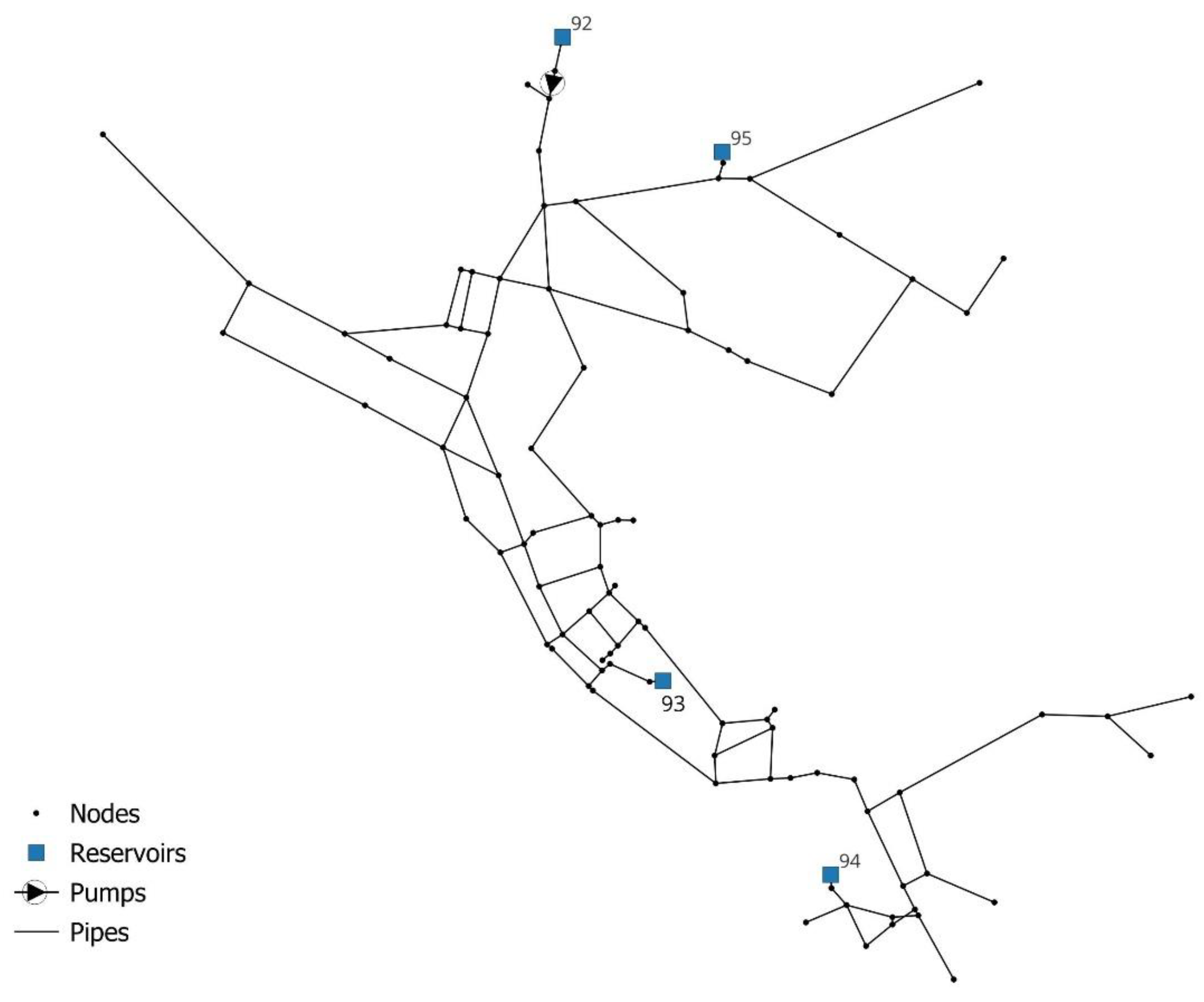
In order to test the validity of the proposed indicator the Wp,n and MPCIi,n values of all the nodes of three real-life WDNs have been computed. The first case is EPANET Net3 system [22], based on North Marin WDN, which is one of the most used networks for validation available in literature; all related data can be found at online database (https://uknowledge.uky.edu/wdsrd/). We analyzed Net3 configuration at 12:00 A.M., as shown in Figure 5. The network has 95 nodes, 4 reservoirs (nodes 92, 93, 94, 95), 115 pipes and 1 pump.
A water scarcity scenario was simulated with the HD approach, where three reservoirs (93, 94, 95) were removed from the WDN and a needle valve with 94,3% opening degree was installed downstream reservoir 92. We compared the results (shown in Figure 6) obtained using the proposed Wp,n and MPCIi,n formulations with the results obtained with the Wp formulation and Hydraulic connectiveness criticality (HCC) indicator, based on structural hole theory, as proposed by Marlim et. al. [20] for WDNs criticality assessment (more details in Supplementary Material).
In Figure 6 pipes are classified in six criticality groups, according to each different indicator (e.g., considering the WDN with 112 pipes, “1%–10%” refers to the first 11 (about 10%) pipes with the highest values of the computed indicator). In Figure 6a and 6c results are shown respectively for Wp,n and MPCIp, while in Figure 6b and 6d results obtained with respectively Wp and HCC formulations [20] are shown:
Figure 6.
North Marin WDN pipes ranked in six criticality groups: e.g., considering the WDN with 112 pipes, “1%–10%” refers to the first 11 (about 10%) pipes with the highest values of the computed indicator. IDs of relevant pipes are depicted in black; head driven (HD) approach was used. Ranking according to: a) Wp,n ; b) Wp (Marlim et. al. [20]) ; c) MPCIp ; d) HCC (Marlim et. al. [20]).
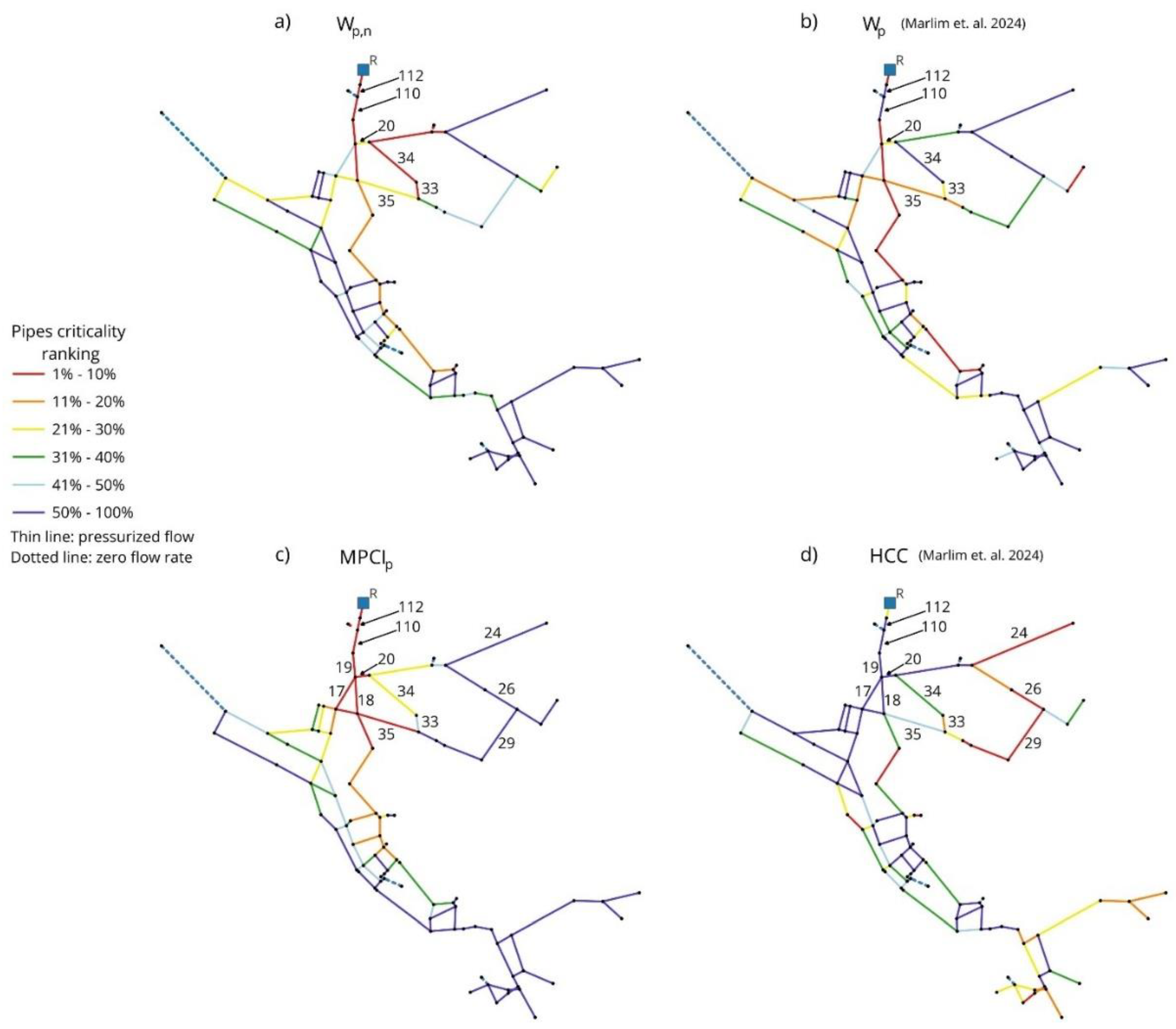
We can observe in Figure 6a and Figure 6b that pipes with the highest Wp,n values (between top 1% and top 10%) are the ones carrying most of the flow in the network and are located downstream of the reservoir and in the central branch of the WDN, while pipes located in peripherals areas generally have low positions in Wp,n ranking.
Pipes 112 and 110, even if located near the reservoir, have zero Wp value (Figure 6b) due to zero nodal demand in each node of these pipes. Instead, with the new Wp,n formulation (Figure 6a), the same pipes rank in the first criticality group because, even though nodal demands are zero, flow rate in these pipes is the highest among all pipes. Eq. (8) correctly captures this criticality, which is also consistent with the topology of the WDN: in fact, a disconnection of these two pipes from the network would lead to hydraulic isolation of all the pipes downstream of the reservoir.
Another significant difference between Figure 6a and Figure 6b is about pipes 33 and 34 where nodal demand in one of their nodes, despite being relatively low, is not satisfied at all: again, this is properly taken into account by Eq. (8) and thus Wp,n is able to provide detailed information about pipes where nodal demand is at least partially not satisfied.
The MPCIp and HCC rankings are shown in Figure 6c and Figure 6d respectively. Unlike Wp,n, that takes into account only hydraulic parameters, MPCIp and HCC integrate topological and hydraulic characteristics and results provide evidence of that.
In Figure 6c pipes 33 and 34 show moderate criticality values, albeit located near pipes with high positions in MPCIp ranking. This can be explained by the relatively low fraction of the total water flow carried by them to the top right area of the WDN. The major fraction is carried instead by pipes 20 and 35, that are the only two connected to both the central branch of the WDN and the top right region: as expected, MPCIp raises up to the first criticality group in spite of Wp,n ranking (Figure 6a) in the third group (21%-30%).
MPCIp and HCC (Figure 6d) criticality rankings are considerably different, especially for pipes 112 and 110 that have the lowest ranking according to HCC formulation (Figure 6d) as a result of the zero nodal demands of their nodes. This criticality also affects pipes downstream of pipe 112 (pipes 17, 18, 19) and lowers their criticality ranking. All these pipes instead, according to MPCIp ranking (Figure 6c), are in the first criticality group as they carry a large portion of flow, and again this is consistent with the topology of the WDN. Considerable differences can also be observed in pipes 24, 26, 29 (top right region in Figure 6c and Figure 6d) that are located in a peripheral region of the WDN: while their HCC ranking is high (Figure 6c), because of their distance from water source and the low number of connected pipes, MPCIp ranking is low, because it gives higher criticality to pipes (like 20 and 35) required by pipes 24, 26 and 29 to remain connected to water sources.
With the aim of quantifying the differences shown in Figure 6, Spearman’s rank correlation coefficient was calculated and results are shown in Table 1:
While a good correlation (rs=0.536) exists between Wp,n and Wp (Marlim et. al. [20]), mainly due to similar computed pipe flows, and also between Wp,n and MPCIp, instead MPCIp and HCC show completely different trends (rs=-0.44), in compliance with criticality rankings depicted in Figure 6c and Figure 6d, because of nodes with zero nodal demands as described above.
In order to give a perspective about how the computed results could lead to a signification variation in water quality, simulations of Net3 were carried out considering a realistic 24h demand pattern, provided in Supplementary Material. Results indicate that, within 24 hours, the velocities in 106 pipes of the 112 pipes are subject to an increase up to 203%. Following Braga et al. [23], we assume that a significant daily velocity variation can lead to systematic detachment of material accumulated over the pipe walls, especially when shear stress on the walls increases significantly. This effect could become more remarkable when a WDN operates for a larger period of time (e.g., during a water scarcity scenario) with several pipes with zero flow rate: when the network returns to regular operating conditions, this would lead to the detachment of all the material accumulated on pipe walls during the previous water scarcity period.
From this first test it is clear that MPCIp accurately integrates hydraulic and topological features of the WDN although even Wp,n alone provides significant insights, especially for free surface flow pipes, that can lead to a significant degradation of the quality of the delivered water.
3.2. Campofelice di Roccella WDN
The second case study is the new WDN designed for the “Campofelice di Roccella” residential area of Sicily, in Italy, shown in Figure 7: the network is modeled with 1 reservoir, 128 nodes and 177 pipes and in the design scenario the flow rate leaving the reservoir is Qsupply =39.2 l/s. In this case results obtained with MP and HD approaches for the hydraulic computations have been compared (for both the proposed Wp,n and MPCIp), in order to highlight the relevant effect of the properly adopted hydraulic solution. In the analyzed water scarcity scenario, a reduced water supply was considered, with a corresponding flow rate Qsupply =30.4 l/s (about 75% of the design water supply) obtained through a needle valve located downstream of the reservoir and a water leakage occurring in each internal node, with a total leakage Qleakage=5.2 l/s (see Supplementary Material for network data).
Figure 7.
Free surface flow pipes and no flow rate pipes computed by a) MP model and b) HD model for Campofelice di Roccella WDN.
Figure 7.
Free surface flow pipes and no flow rate pipes computed by a) MP model and b) HD model for Campofelice di Roccella WDN.
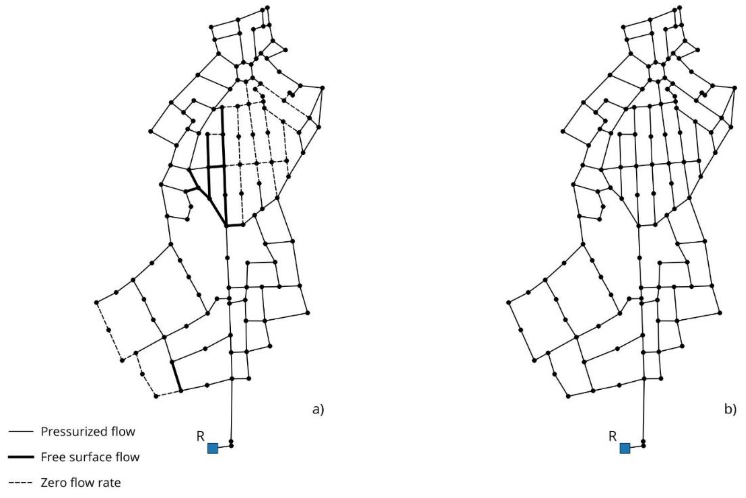
In this scenario remarkable differences appear between the two models: while the HD model (Figure 7b) provides zero pipes with no flow rate, the MP model (Figure 7a) provides 13 pipes with free surface flow and 36 pipes with no flow rate, which represent about 20% of the total number of pipes in the WDN. These results directly impact Wp,n and MPCIp ranking for both models, as shown in Figure 8:
The most critical pipes for Wp,n and MPCIp rankings are, as expected, the ones near the reservoir and in the central area of the WDN, followed in the ranking by their adjacent pipes.
In particular Wp,n rankings do not differ significantly between MP (Figure 8a) and HD (Figure 8b) models in key regions of the network, due to the high number of pipes where nodal demands of their nodes are not partially or completely satisfied: this shows clearly how Wp formulation of Eq. (8) is able to identify critical pipes from an hydraulic point of view and it is not strongly affected by the adopted hydraulic model, although pipes where free surface flow occurs generally have an higher ranking with MP model (Figure 8a) than with the HD one (Figure 8b). Observe that, due to water leakage in nodes, qp increases in some pipes and Wp,n increases as well: this is consistent because criticality of these pipes has to take into account the effect of leakage; as a consequence, only the actual nodal flow, excluding leakages, is considered in Qa,i and Qa,j of Eq. (8).
Figure 8.
Campofelice di Roccella WDN pipes ranked in six criticality groups depending on the considered indicator: e.g., considering the WDN with 177 pipes, “1%–10%” refers to the first 17 (about 10%) pipes with the highest values of the computed indicator. IDs of relevant pipes are depicted in black. Ranking according to: a) Wp,n (MP approach) ; b) Wp,n (HD approach) ; c) MPCIp (MP approach) ; d) MPCIp (HD approach).
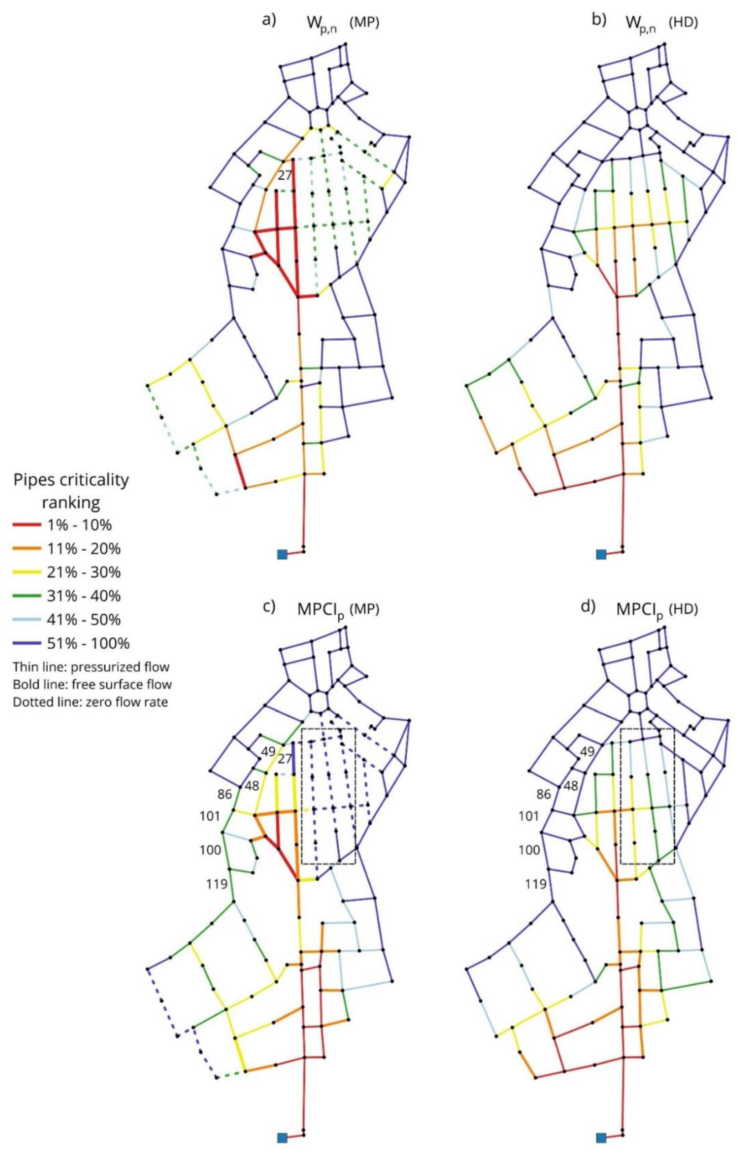
However, the results provided by MPCIp offer a very different perspective on the criticality ranking: in fact, according to HD model (Figure 8d), there is an entire group of pipes, located in the central WDN area (identified by the dotted box in Figure 8d), with a rank between the third and fifth group of criticality. This is because HD model is unable to estimate the zero flow rate in this area, computed instead by the MP model as shown before in Figure 7a.
According to the HD model, these pipes have a major relevance, because they carry the major fraction of flow to the upper part of the WDN. The pipes in the external areas of the network are instead ranked in the least critical group (49, 48, 86, 101, 100, 119 on the left in Figure 8d).
The MP model, on the opposite (Figure 8c), is able to detect free surface flow pipes and in particular pipes with zero flow rate, and this leads to substantially different results: a significant variation in criticality ranking affects almost all the pipes in the central region of the WDN (dotted box in Figure 8c), that rank in the least criticality group even though, from just an hydraulic point of view, they are quite critical (as attested by high Wp,n ranking in Figure 8a). These pipes are in fact no more essential in the considered scenario, because a large part of the entering flow is redirected to a different part of the network, specifically to pipes on the left side (49, 48, 86, 101, 100, 119). All these pipes show now greater relevance and they are essential for the water supply of the upper part of the network that, according to the MP model, cannot be supplied by the central WDN region anymore.
This relevant difference in criticality ranking is caused by several adjacent pipes in the central region with zero flow rate: the nodes connecting these pipes will have a zero CWF value (Eq. (11)), because their number nℜ of reachable nodes is equal to zero and, as consequence, their MPCIi decreases dramatically or even drops to zero. This also proves that CWF(i) is necessary in Eq. (12) because otherwise, if the influence of node i were only given by C(i)-1 (and not by C(i)-1CWF(i)) than node i would always have much higher influence than all the other connected nodes (given by ) due to the higher order or magnitude of C(i)-1.
A final consideration concerns pipe 27 which, despite being in the first criticality group in Wp,n ranking (Figure 8a), in MPCIp ranking is in the last group (Figure 8c): this major variation is the effect of zero or low flow rate in all the pipes connected to pipe 27. This is correctly taken into account by MPCIp formulation (Eq. 12); again, as mentioned before, low MPCIp ranking suggests that pipe 27 role is not fundamental for the WDN in the analyzed scenario.
Spearman’s coefficient results are provided in Table 2:
Results confirm what shown in Figure 8, in particular a strong correlation (rs=0.903) can be observed between the hydraulic weight Wp,n and MPCIp. The reason is that HD approach is unable to determine free surface flow pipes, unlike the MP approach, and this leads to a smaller correlation (rs=0.478).
3.3. Marchi Rural WDN
A third test case is the Marchi Rural water distribution network in Australia, based on a real irrigation system, which can be classified as a transmission dense-loop network, unlike the first two analyzed WDNs. The network has 2 reservoirs, 380 nodes and 477 pipes; data can be found at online database (https://uknowledge.uky.edu/wdsrd/).
In this test only a regular scenario, where all nodal demands are satisfied, was analyzed, and the HD approach was used for the hydraulic model.
In Figure 9a comparison between the hydraulic weight computed according to Marlim et. al. [20] and according to the new formulation of Eq. (9) can be observed:
Major differences are evident between Figure 9a and Figure 9b and this is mainly due to the large number of nodes with zero nodal demand. In fact, when both nodes of one pipe have zero demand, the computed pipe hydraulic weight (Marlim et. al. [20]) will always be zero, regardless of the pipe flow which instead could be very high, especially near the two reservoirs (R1 and R2) and in critical pipes connecting separated areas of the WDN. Because of this, in Figure 9a the real hydraulic dynamics of the network cannot be observed, and the most critical pipes (depicted in red in Figure 9a) are always the ones located in the most peripherical areas of the WDN, irrespective of every other parameter.
Figure 9.
Marchi Rural WDN pipes ranked in six criticality groups depending on the considered indicator: e.g., considering the WDN with 477 pipes, “1%–10%” refers to the first 47 (about 10%) pipes with the highest values of the computed indicator. IDs of relevant pipes are depicted in black; head driven (HD) approach was used. Ranking according to: a) Wp (Marlim et. al. [20]) ; b) Wp,n.
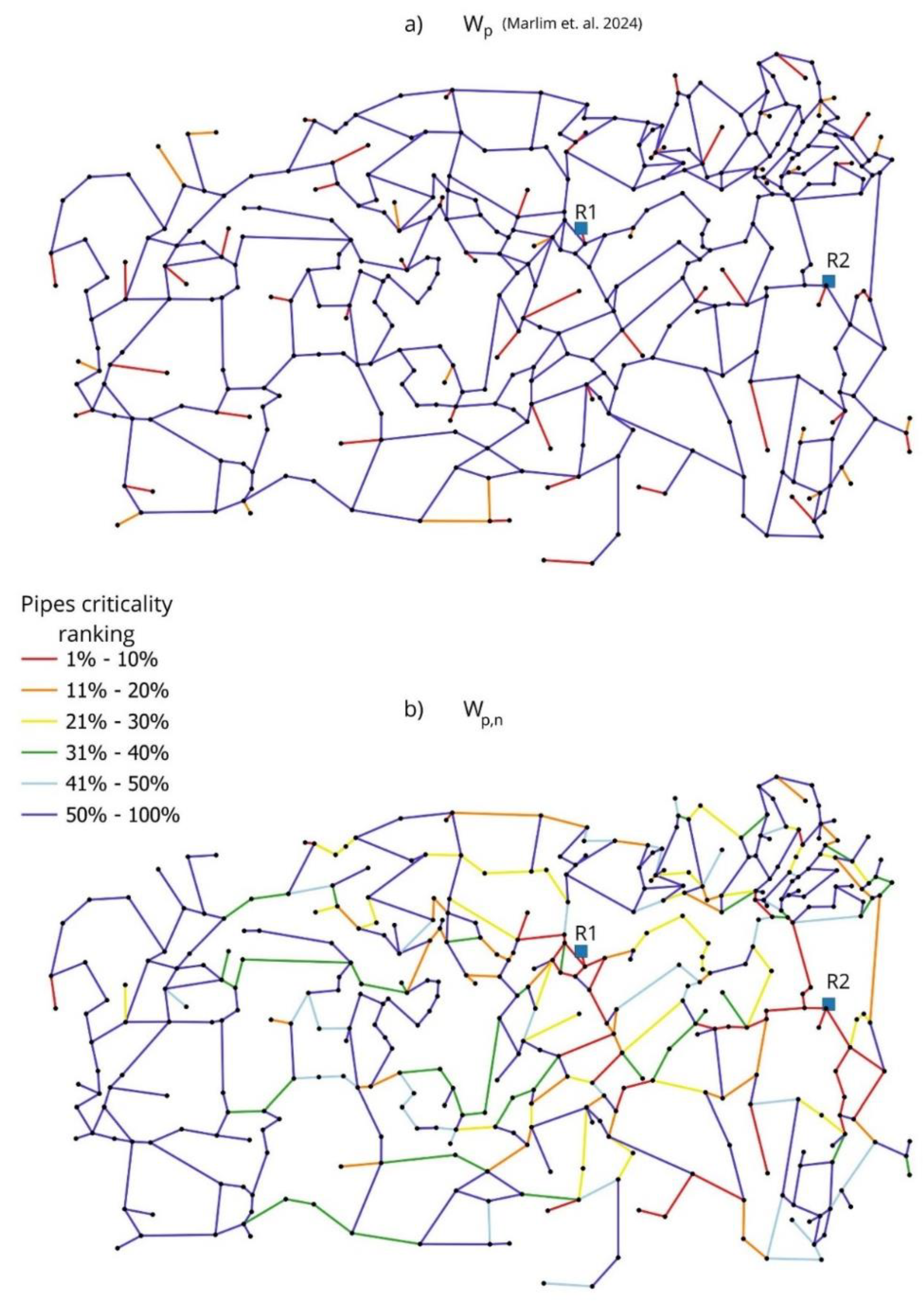
Formulation of Eq. (9) instead correctly captures the hydraulic dynamics and, as expected, the most critical pipes are those located near the reservoirs, while medium criticality (between the top 21%–30% and top 31%–40% Wp,n) is assigned to pipes acting as a bridge between different regions of the network.
This test clearly shows that the new formulation performs accurately even in scenarios where only few nodes have higher than zero demand; finally, even though only the HD approach was applied, results are consistent with water dynamics and again this proves that the new hydraulic weight does not necessarily need to always rely on MP approach.
4. Conclusions
A new indicator for WDNs criticality assessment is developed, integrating the Minimum Pressure (MP) approach, which relies on the assumption that the minimum pressure inside the network remains always greater or equal to zero. The new MPCI indicator relies also on the new defined hydraulic pipe weight Wp, that embeds both nodal and link parameters, according to the structural hole theory. In the three analyzed test cases numerical results show that MPCI can usually provide a reliable estimate of the most critical pipes even using a standard Head Driven (HD) approach for hydraulic modeling. In the case of water scarcity scenario, the use of MP modeling approach leads to very different outcomes with respect to the classical head driven approach and this results into a different prioritized maintenance schedule for pipes.Finally observe that well designed WDNs never attain, with the design nodal flows, negative pressures. In this case, MP approach provides the same results of the head driven model. On the other hand, the assumption of failure of one or more network components could lead to significantly different outcomes for the proposed criticality indicator between MP model and other WDNs models.The computed results call for further improvements of the proposed methodology and for further tests of the MPCI indicator, especially in more complex networks with multiple sources and valves, by analyzing the impact that valves’ isolation has on the WDN hydraulic dynamics and the effect that the resulting variations of the flow distribution have on the proposed indicator. MPCI could also be incorporated in water quality studies to determine the relationship between water quality and the velocity variations during long time periods, particularly in the event of a network segment’s isolation, that could lead to unexpected flow direction change in pipes. Finally, the proposed indicator could be implemented as an objective function in the planning of new WDNs, to optimize their layout and to increase their reliability.
Supplementary Materials
The following supporting information can be downloaded at the website of this paper posted on Preprints.org.
Author Contributions
Conceptualization, D.P., M.S., and T.T.; methodology, D.P., M.S; software, D.P., C.P.; validation, D.P., M.S.; formal analysis, D.P.; investigation, D.P., M.S.; resources, D.P., M.S.; data curation, D.P.; writing—original draft preparation, D.P.; writing—review and editing, D.P., M.S., C.P., T.T.; visualization, D.P., M.S.; supervision, M.S., T.T.; project administration, D.P., T.T.; funding acquisition, T.T. All authors have read and agreed to the published version of the manuscript.
Funding
This research received no external funding.
Data Availability Statement
Data is contained within the article or supplementary material.
Conflicts of Interest
The authors declare no conflicts of interest.
Abbreviations
The following abbreviations are used in this manuscript:
| WDN | Water Distribution Network |
| MP | Minimum Pressure |
| WPI | Water Performance Indicator |
| HD | Head Driven |
| MPCI | Minimum Pressure Criticality Indicator |
References
- Alegre, H.; Baptista, J.M.; Cabrera, E.; Cubillo, F.; Duarte, P.; Hirner, W.; Merkel, W.; Parena, R. Performance Indicators for Water Supply Services: Third Edition. Water Intelligence Online 2016, 15, 9781780406336. [Google Scholar] [CrossRef]
- Li, P.-H.; Kao, J.-J. Segment-Based Vulnerability Analysis System for a Water Distribution Network. Civil Engineering and Environmental Systems 2008, 25, 41–58. [Google Scholar] [CrossRef]
- Walski, T.M. Water Distribution Valve Topology for Reliability Analysis. Reliability Engineering & System Safety 1993, 42, 21–27. [Google Scholar] [CrossRef]
- Yazdani, A.; Jeffrey, P. Water Distribution System Vulnerability Analysis Using Weighted and Directed Network Models. Water Resources Research 2012, 48. [Google Scholar] [CrossRef]
- Abdel-Mottaleb, N.; Walski, T. Evaluating Segment and Valve Importance and Vulnerability. Journal of Water Resources Planning and Management 2021, 147. [Google Scholar] [CrossRef]
- Liu, J.; Kang, Y. Segment-Based Resilience Response and Intervention Evaluation of Water Distribution Systems. Journal of Water Supply Research and Technology—AQUA 2021, 71, 100–119. [Google Scholar] [CrossRef]
- Tornyeviadzi, H.M.; Neba, F.A.; Mohammed, H.; Seidu, R. Nodal Vulnerability Assessment of Water Distribution Networks: An Integrated Fuzzy AHP-TOPSIS Approach. International Journal of Critical Infrastructure Protection 2021, 34, 100434. [Google Scholar] [CrossRef]
- Marlim, M.S.; Jeong, G.; Kang, D. Identification of Critical Pipes Using a Criticality Index in Water Distribution Networks. Applied Sciences 2019, 9, 4052. [Google Scholar] [CrossRef]
- Giustolisi, O.; Ridolfi, L.; Simone, A. Tailoring Centrality Metrics for Water Distribution Networks. Water Resources Research 2019, 55, 2348–2369. [Google Scholar] [CrossRef]
- Tucciarelli, T.; Puleo, D.; Nasello, C.; Sinagra, M. A minimum pressure approach for water distribution network modelling, Water Resources Management 2024. [CrossRef]
- Shin, G.; Kwon, S.H.; Lee, S. Designing Isolation Valve System to Prevent Unexpected Water Quality Incident. Sustainability 2023, 16, 153. [Google Scholar] [CrossRef]
- Husband, S.; Boxall, J. Understanding and Managing Discolouration Risk in Trunk Mains. Water Research 2016, 107, 127–140. [Google Scholar] [CrossRef] [PubMed]
- Boxall, J.B.; Saul, A.J. Modeling Discoloration in Potable Water Distribution Systems. Journal of Environmental Engineering 2005, 131, 716–725. [Google Scholar] [CrossRef]
- Zhu, C.; Wang, X.; Zhu, L. A Novel Method of Evaluating Key Nodes in Complex Networks. Chaos Solitons & Fractals 2017, 96, 43–50. [Google Scholar] [CrossRef]
- Burt, R.S. Structural Holes: The Social Structure of Competition. SSRN Electronic Journal 1992. [Google Scholar]
- Lazega, E.; Burt, R.S. Structural Holes: The Social Structure of Competition. Revue Française De Sociologie 1995, 36, 779. [Google Scholar] [CrossRef]
- Burt, R.S. The Network Structure of Social Capital. Research in Organizational Behavior 2000, 22, 345–423. [Google Scholar] [CrossRef]
- Burt, R.S. Structural Holes versus Network Closure as Social Capital. In Routledge eBooks; 2017; pp. 31–56.
- Yang, E.; Faust, K.M. Quantifying the Impact of Population Dynamics on the Structural Robustness of Water Infrastructure Using a Structural Hole Influence Matrix Approach. ACS ES&T Water 2022, 2, 1161–1173. [Google Scholar] [CrossRef]
- Marlim, M.S.; Kang, D. Hydraulic Connectiveness Metric for the Analysis of Criticality in Water Distribution Networks. Water 2024, 16, 1498. [Google Scholar] [CrossRef]
- Wasserman, S.; Faust, K. Social Network Analysis: Methods and Applications; 1994. [Google Scholar]
- Clark, R.M.; Rossman, L.A.; Wymer, L.J. Modeling Distribution System Water Quality: Regulatory Implications. Journal of Water Resources Planning and Management 1995, 121, 423–428. [Google Scholar] [CrossRef]
- Braga, A.S.; Saulnier, R.; Filion, Y.; Cushing, A. Dynamics of Material Detachment from Drinking Water Pipes under Flushing Conditions in a Full-Scale Drinking Water Laboratory System. Urban Water Journal 2020, 17, 745–753. [Google Scholar] [CrossRef]
Figure 1.
pij computed for a node and its neighboring nodes.
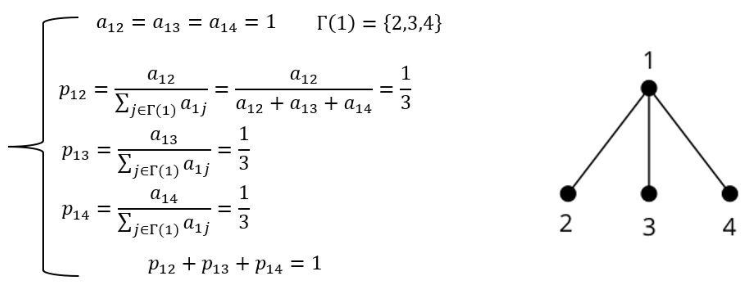
Figure 2.
Wp,n computed in a simple network. Pipes are colored depending on their Wp,n value.
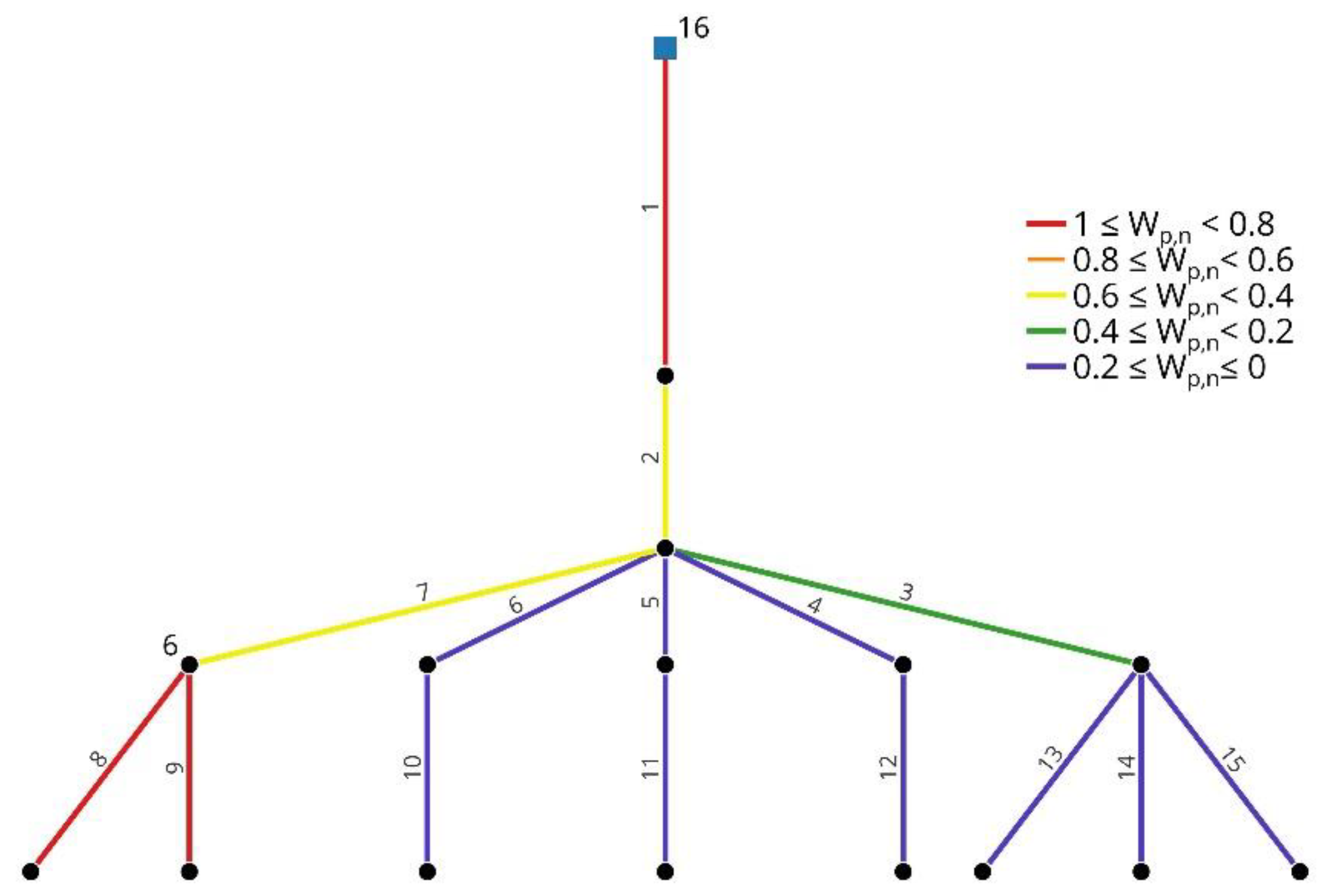
Figure 3.
CWF calculation for node 6 of Figure 2. Arrows in pipes show flow direction; the shortest paths crossing node 6 between source node (16) and target nodes (14,15) are highlighted in blue.
Figure 3.
CWF calculation for node 6 of Figure 2. Arrows in pipes show flow direction; the shortest paths crossing node 6 between source node (16) and target nodes (14,15) are highlighted in blue.
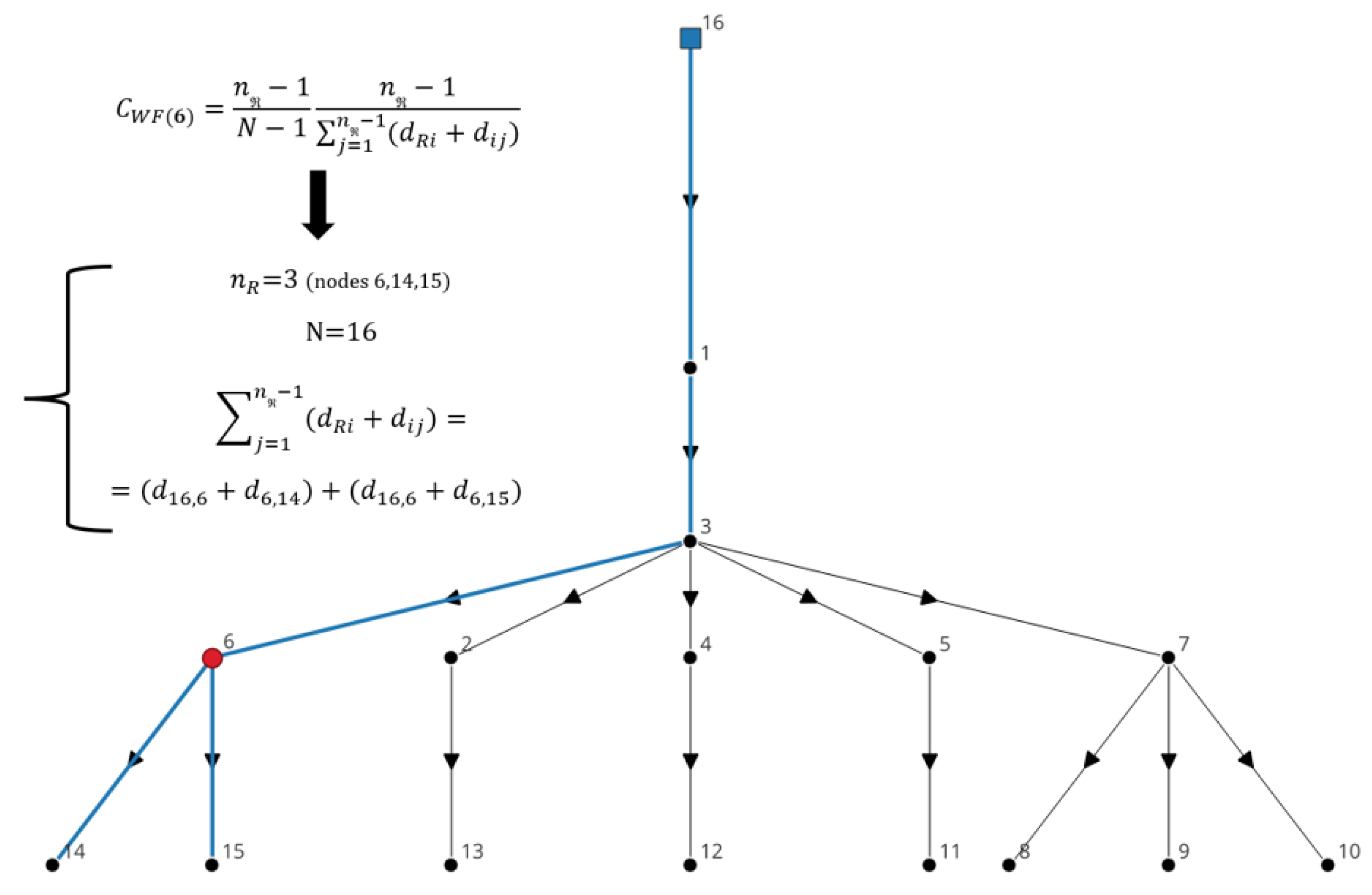
Figure 4.
MPCIp flowchart.
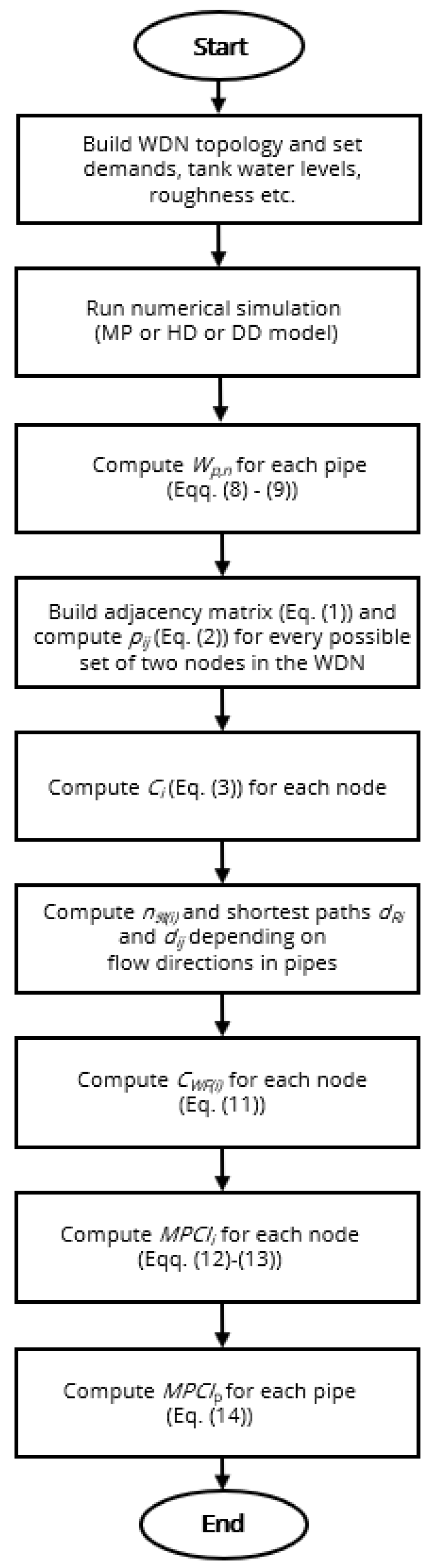
Figure 5.
Net3 configuration at 12:00 A.M.

Disclaimer/Publisher’s Note: The statements, opinions and data contained in all publications are solely those of the individual author(s) and contributor(s) and not of MDPI and/or the editor(s). MDPI and/or the editor(s) disclaim responsibility for any injury to people or property resulting from any ideas, methods, instructions or products referred to in the content. |
© 2025 by the authors. Licensee MDPI, Basel, Switzerland. This article is an open access article distributed under the terms and conditions of the Creative Commons Attribution (CC BY) license (https://creativecommons.org/licenses/by/4.0/).
Copyright: This open access article is published under a Creative Commons CC BY 4.0 license, which permit the free download, distribution, and reuse, provided that the author and preprint are cited in any reuse.


