
Submitted:
03 November 2025
Posted:
05 November 2025
You are already at the latest version
Abstract
To address the challenges posed by increased power consumption in traditional active relays and the difficulties associated with countering channel fading for Intelligent Reflecting Surfaces (IRS), we propose a dual-mode relay (DMR) capable of dynamically switching between two operational modes: active relaying and passive IRS reflection. This DMR allows its units (DMRU) to select their operational modes dynamically based on channel conditions, enabling the transmission of composite-mode signals that consist of both active relaying signal components and IRS-reflected components, thereby enhancing adaptation to the wireless environment. Furthermore, under the constraint of limited transmit power, we introduce a DMR-based Adaptive Transmission (DMRAT) method. This approach explores all possible DMR operational modes and employs the Alternating Optimization (AO) algorithm in each mode to jointly optimize the beamforming matrices of both the transmitter and the DMR, along with the reflection coefficient matrix of the IRS. Consequently, this maximizes the data transmission rate for the target communication pair. The optimal DMR mode can then be determined based on the optimized data rate for the target communication across various operational modes. Simulation results demonstrate that the proposed method significantly enhances the data transmission rate for the target communication pair.
Keywords:
Intelligent Reflecting Surface
; relay
; beamforming
; adaptive transmission
1. Introduction
The rapid advancement of wireless communication technologies has led to a significant increase in both the number of users and the traffic load within communication systems. To provide high-quality data services to mobile users, ensuring adequate network coverage is essential. Relay technology, which employs relay nodes to receive and forward signals, can extend communication range and enhance users’ signal reception quality [1]. Decode-and-Forward (DF) and Amplify-and-Forward (AF) are two of the most prevalent relaying schemes in this domain. However, these conventional active relay technologies fundamentally rely on active components, including carrier signal generators, analog-to-digital converters, and power amplifiers [2], resulting in substantial hardware complexity and significant power consumption. Intelligent Reflecting Surfaces (IRS) consist of numerous passive reflecting elements, each capable of dynamically adjusting its reflection coefficient under the control of an IRS controller to modify both the amplitude and phase of the incident signal. As a low-cost, flexibly deployable, and fully passive device, IRS can be applied in various domains such as physical-layer security [3,4,5,6] and enhancement of wireless data transmission [7,8]. It is regarded as a revolutionary technology in the field of wireless communications, offering new design paradigms for signal forwarding and relaying.
Although there has been considerable theoretical and practical research on IRS, their limited signal processing capabilities and passive nature make them more susceptible to channel fading. Moreover, practical implementations of IRS encounter constraints such as limited operating frequency bands [9] and insufficient dynamic adjustment capabilities [10]. Consequently, some research efforts have shifted toward integrated designs that combine IRS with relay techniques. The authors of [11] investigated an IRS-assisted two-way Amplify-and-Forward (AF) relaying system, where one IRS is deployed between the transmitter and the relay node, and another is positioned between the relay and the receiver to enhance signal transmission. By optimizing the phase shift matrices of both IRSs, the signals forwarded by the relay and those transmitted from the source are constructively superimposed in phase at the destination receiver, thereby reducing the bit-error rate (BER). In [12], the authors proposed a UAV-aided communication scheme that jointly employs an active relay and an IRS. In this study, the UAV is equipped with a multi-antenna AF relay and an IRS consisting of multiple passive reflecting elements, which operate both independently and collaboratively to forward signals. Through joint optimization of the UAV’s trajectory, the IRS reflection coefficients, and the relay beamforming parameters, the achievable data rate at the target receiver is maximized.
Despite the studies in [11,12] that integrate IRS with relays, they primarily treat the passive IRS as a supplementary tool to enhance the performance of active relays, without considering the flexible replacement of active relays by IRS (i.e., the adaptive selection between relay and IRS). In fact, both relay and IRS have their own advantages and disadvantages regarding energy efficiency, hardware and computational complexity, and coverage. The ability to adaptively replace active relays with passive IRS based on dynamic wireless channel conditions—which can either reduce power consumption or enhance data transmission under fixed power constraints—holds significant research importance for improving communication performance from the source to the destination node. Therefore, this paper proposes a dual-mode relay (DMR) capable of dynamically switching between an active relaying mode and a passive IRS reflection mode. The DMR consists of multiple dual-mode relay units (DMRU), each of which can flexibly switch between active relaying and passive IRS reflection based on wireless channel conditions. Multiple DMRUs cooperatively process the incident signal in a composite manner to relay data information. Furthermore, under a transmit power constraint, we design a DMR-based Adaptive Transmission (DMRAT) scheme. This scheme evaluates all possible DMR operational modes and, for each mode, jointly optimizes the beamforming matrix at the transmitter and the operational parameters of the DMRUs operating in either active or passive mode using an Alternating Optimization (AO) algorithm, with the goal of improving the data rate at the receiver.
The rest of this paper is organized as follows. Section 2 describes the system model, while Section 3 presents the design of DMRAT. Section 4 evaluates the performance of the proposed method. Finally, we conclude this paper in Section 5.
Throughout this paper, we will use the following notations. The set of complex numbers is denoted as , while vectors and matrices are represented by lower-case and upper-case bold letters. and represent matrix transpose and conjugate transpose, respectively. denotes the absolute value of a complex number.
2. System Model
We consider a communication system consisting of one transmitter (Tx), one receiver (Rx), and a dual-mode relay (DMR), as illustrated in Figure 1. The Tx is equipped with antennas and transmits with power , while the Rx has antennas. Due to obstacles or severe channel fading between the Tx and Rx, no direct link satisfying the transmission quality requirement is available [13]. The DMR consists of DMRUs, each capable of dynamically switching between active relaying and passive IRS reflection modes for signal forwarding, under the control of a control unit (CU) co-located with the Tx. When a DMRU operates in active relaying mode, it functions as a full-duplex DF relay. The total transmit power consumed by the DMR is denoted as . Assuming that the signal processing delays for both DF relaying and passive IRS reflection are negligible, the signals actively forwarded and passively reflected by all DMRUs can arrive at the Rx simultaneously.
Prior to communication, the Tx broadcasts a pilot signal with all DMRUs of the DMR operating in passive IRS reflection mode. The Rx estimates the Channel State Information (CSI) [14] between itself and both the IRS and the Tx, denoted as and in Figure 1, and feeds this information back to the Tx. The Tx then transmits the data . The Tx precodes using the beamforming matrix and then map the pre-processed output to the transmit antennas for transmission. The channels between the Tx and the DMR, and between the DMR and the Rx, are represented by and , respectively. We employ a spatially uncorrelated Rayleigh flat fading channel model to characterize these channels, where the elements are independent and identically distributed complex Gaussian random variables with zero mean and unit variance. Both and exhibit quasi-static flat fading [15] characteristics.
3. Design of DMRAT
This section presents the design of the DMRAT under the constraint of the total transmit power at both the Tx and the DMR. For simplicity, we assume , where M is a positive integer.
3.1. Basic Signal Processing in the DMR
In practical applications, when the channel quality from the Tx to the Rx via the IRS is sufficiently good, the DF relay may not be necessary. In such cases, using only IRS reflection can provide the Rx with adequate signal reception quality. Conversely, when the channel condition is poor, using IRS reflection alone may not be sufficient to ensure good reception quality at the Rx. Therefore, it is necessary to set some DRMUs to active relaying mode to compensate for channel fading, albeit at the cost of some transmit power. To reduce the power consumption of the DMR, the Tx can configure a subset of the DMRUs to operate in IRS mode. As a result, some DMRUs operate in DF relaying mode, while others function in passive IRS reflection mode. The Rx then receives a composite signal constructed from multiple signal components originating from the DMRUs operating in these two distinct modes. To control the operating modes of the M DMRUs in the DMR, we define a mode selection matrix , where each element () indicates whether the m-th DMRU operates in DF relaying mode or IRS reflection mode.
Let denote the m-th DMRU. We define as the set of DMRUs operating in DF relaying mode and as the set of DMRUs operating in IRS reflection mode. holds, where represents the entire set of DMRUs. For each , the mode indicator is set as ; conversely, for , . Under the control of the mode selection matrix , the received signal at the Rx can be expressed as:
The first term on the right-hand side (RHS) of Equation (1) represents the signal forwarded by the DMRUs operating in the DF relaying mode, while the second term corresponds to the signal reflected by the DMRUs operating in the IRS reflection mode. denotes the beamforming matrix for the DMRUs in , where is the m-th column vector of . represents the AWGN vector, whose elements have zero mean and variance . The reflection coefficient matrix of the DMRUs in is represented as , where and denote the phase coefficient and amplitude coefficient, respectively, of the m-th DMRU operating in IRS mode. represents the beamforming matrix at the Tx. The matrices and (where is the identity matrix and ⊕ denotes element-wise modulo-2 addition) are applied to and , respectively, to select the operating mode of each DMRU. When , the matrix sets the m-th row elements of to zero; when , sets the m-th reflection coefficient in to zero, i.e., .
Under the total transmit power constraint , we let for example. The subsequent analysis can be applied to other power allocations. The Rx employs a filtering matrix for post-processing the received signal , where is the filter vector corresponding to the desired data . The estimated signal can be expressed as . The data rate at the Rx is calculated as:
where and are the m-th row vectors of the equivalent channel matrices and , respectively. The matrix represents the channel between the Rx and the DMRUs operating in DF relaying mode, while represents the channel associated with the DMRUs operating in IRS mode.
3.2. Design of DMR’s Operating Parameters
To maximize the data rate under the total power constraint , it is essential to optimize the mode selection matrix and jointly design the beamforming matrices , , and the reflection coefficient matrix . To achieve this object, we first derive the optimal , , and that maximize for a fixed , leading to the optimization problem expressed in Equation (3):
We assume that both and are entirely allocated to the data transmission of the target Tx–Rx pair, and that the processing at the Tx and the DF relaying mode DMRUs does not introduce additional gain to the transmitted signal; i.e., and hold. Subsequently, for a given total transmit power , we configure different mode selection matrices and employ the AO algorithm to solve the optimization problem given in Equation (3). The main idea of the algorithm is as follows. First, initialize and design both and accordingly. Then, based on the determined and , optimize . Subsequently, with the newly obtained , redesign and . This process iterates until the improvement in falls below a predefined threshold, or the number of iterations exceeds a preset maximum value, at which point the algorithm terminates. Thus, for a given , we can compute a set of , , and that maximizes . In what follows, we will elaborate on the method for computing the DMR’s operating parameters using AO under a fixed .
3.2.1. Design of Beamforming at the Tx and DMR
First, we initialize (i.e., set and ), and apply Zero-Forcing Beamforming (ZFBF) [16] to design and . This method effectively eliminates mutual interference among multiple concurrent signals, thereby improving data transmission performance. Under this initialization, Equation (3) can be rewritten as:
We use to denote the m-th column vector of the matrix , and to represent the m-th column vector of . Then, the m-th column of the precoding matrix , denoted as , can be obtained as , where represents the Frobenius norm of a vector or matrix. Similarly, the m-th column of can be calculated as .
3.2.2. Design of the IRS’s Reflection Coefficient Matrix
After computing and , Equation (4) becomes:
Based on the definition of and Equation (2), when , the selection matrix sets the m-th row of to zero, resulting in . Conversely, when , the operation sets the m-th main diagonal element of to zero (i.e., ), which implies . Substituting and into Equation (2) leads to:
where . Note that the first term on the RHS of Equation (6) does not contain the unknown parameter . Therefore, only the second term on the RHS of Equation (6) needs to be optimized. Consequently, Equation (5) can be equivalently expressed as:
We can derive , where denotes the element at the m-th row and m-th column of a matrix. Given that and , we can have:
Substituting into Equation (8) and simplifying, we obtain . Since is a symmetric matrix, holds; therefore, . As a result, can be simplified as:
According to Jensen’s inequality, we have:
Note that reaches its maximum value if and only if all non-zero main diagonal elements of in Equation (10) are equal; this condition can also maximize . Suppose that after optimizing , all non-zero main diagonal elements of become , achieving the maximum . It is observed that when , all non-zero main diagonal elements of are exactly ; therefore, the condition can be used as a constraint for optimizing . Furthermore, using the property of diagonal matrices, we have . Thus, to maximize , it is necessary to solve for such that holds. The computation procedure is detailed as follows.
By expanding in , we can rewrite as:
Here, is the m-th row vector of , and . According to Equation (11), we get:
where is defined as .
Left-multiplying both sides of Equation (12) by the left pseudo-inverse of , defined as , and then right-multiplying by the right pseudo-inverse of , expressed as , we obtain:
Expanding the term on the left-hand side (LHS) of Equation (13), and noting that all matrices on the RHS are known without containing any unknown parameters, we can calculate the RHS of Equation (13) and denote the result as . Thus, we have:
where ( indicate the relative position of within ) is a diagonal matrix whose non-zero main diagonal elements are equal (denoted as ). Since , the main diagonal elements of satisfy . Therefore, the corresponding of must also satisfy . By defining , the condition is satisfied. From Equation (14), we can derive , which allows us to establish a set of equations for the unknown variables and as follows:
where . When , is a real number; otherwise, is complex. Equation (15) comprises a total of independent equations with unknowns, thus leading to infinitely many solutions. The general solution of Equation (15) for the unknown variables can be expressed as:
where . To obtain a particular solution, we can assign an arbitrary value to any one of (e.g., ); afterwards, the values of the remaining for can be computed using Equation (16).
Subsequently, and are recalculated under the current optimized . Using these updated beamforming matrices, is then re-optimized. This process continues iteratively until the improvement in —defined as the difference between and obtained in the l-th and -th iterations—falls below a predefined threshold , or until the iteration count l reaches the maximum value . The selection of influences the algorithm’s performance and efficiency: a value too large may cause premature termination, resulting in suboptimal data rate performance, while a value too small can yield better optimization at the expense of prolonged convergence. In this work, is chosen based on simulation studies. To summarize, we present the AO procedure for jointly determining , , and in Algorithm 1.
| Algorithm 1 AO-based Joint Optimization of , , and |
|
3.2.3. Selection of DMR Operating Mode
For the DMR operating mode selection matrix , since the DMR contains M DMRUs and has a total of distinct operating modes, it is necessary to perform joint optimization of , , and using the AO technique for each possible to maximize . Then, by comparing across different configurations, the configuration that yields the highest is selected.
4. Evaluation
This section employs MATLAB simulation to evaluate the performance of the DMRAT scheme. The total transmit power is set to , with . Note that when all DMRUs operate in IRS passive reflection mode, , and accordingly we configure . We define the transmit power normalized by noise power as dB, and set dB for the simulation. We use Monte Carlo simulation with 1500 independent trials. In each trial, the channels and are generated randomly.
Figure 2 illustrates the variation of the data rate performance at the Rx along with for different values of M. We denote the proposed DMRAT using AO as DMRAT-AO, and compare it with three other schemes: DMR-IRS (where all DMRUs adopt passive IRS reflection mode), DMR-DF (where all DMRUs adopt DF relaying mode), and DMR-R (where all DMRUs randomly adopt either passive IRS reflection mode or DF relaying mode). As the figure shows, the data rates of all methods increase with the growth of M. This is due to the improved signal processing gain provided by multiple antennas. For a fixed M, DMRAT-AO outperforms the other three methods in the achievable data rate. This is because DMRAT-AO utilizes AO to jointly optimize the operating parameters of both the Tx and the DMR, selecting the optimal operating mode for the DMR to maximize the data rate at the Rx. DMR-DF employs the DF relaying mode to decode and forward the signal transmitted by the Tx, effectively compensating for channel fading through the consumption of transmit power. Moreover, in this study we assume that the DF relay can decode the signal from the Tx without errors; hence, the rate performance of DMR-DF is influenced solely by the channel between the DMR and the Rx. In other words, under the total transmit power constraint , DMR-DF allocates half of to the Tx, ensuring reliable communication from the Tx to the DMR. In contrast, DMR-IRS allocates all transmit power to the Tx, and its data rate performance at the Rx is cooperatively affected by the channel fading between the Tx and DMR, as well as the DMR and Rx. Poor quality in either of these two links will degrade the data rate of DMR-IRS. Therefore, given the same , DMR-DF significantly outperforms DMR-IRS, which exhibits the poorest rate performance. DMR-R randomly selects the operating mode of each DMRU. When channel conditions are poor, inappropriate selection of the IRS mode may lead to reduced data rate at the Rx. As a result, the rate performance of DMR-R is inferior to that of DMR-DF.
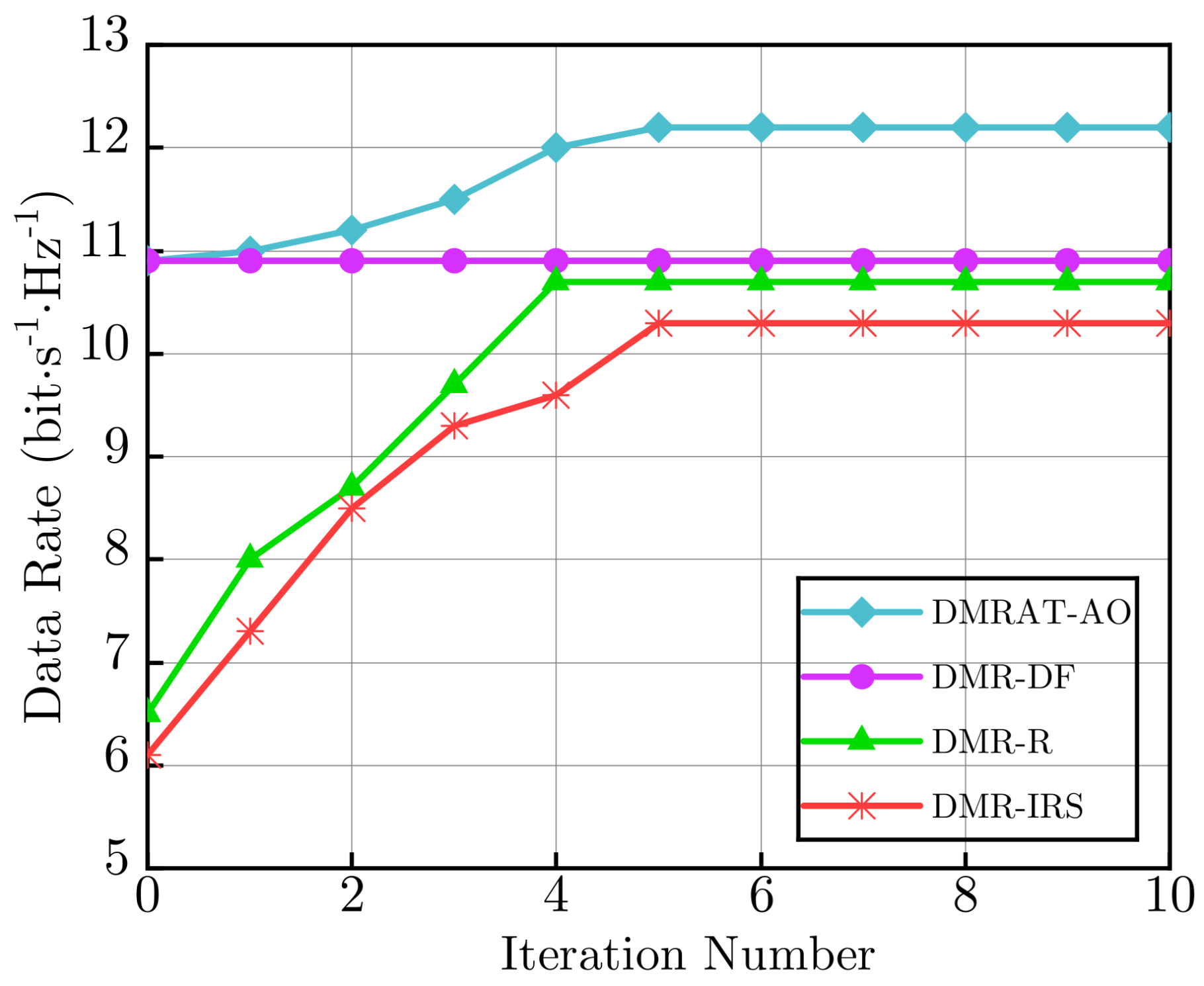
Figure 3 shows the data rate at the Rx versus the number of iterations under for different DMR operating modes. When all DMRUs operate in DF relaying mode, only ZFBF is required to design and , without needing to compute or apply AO. Therefore, the data rate achieved by DMR-DF remains unchanged as the number of iterations increases. In contrast, the data rate of DMRAT-AO gradually increases during the first five iterations, consistently outperforming the other methods, and converges after approximately five iterations. The data rate of DMR-IRS stabilizes after five iterations, while that of DMR-R ceases to improve after four iterations. This is because DMRAT-AO uses AO to select the DMR operating mode that maximizes the data rate at the Rx, resulting in superior performance. Additionally, at the initial iteration (i.e., ), since DMRAT-AO sets initial operating state of the DMR to DMR-DF, the data rates of DMRAT-AO and DMR-DF are identical when .
5. Conclusion
To address the challenges of high power consumption in active relays and the limited fading resistance of passive IRS, this paper proposes a dual-mode relay (DMR) capable of dynamically switching between active relaying and passive IRS reflection modes according to channel conditions. Under a total transmit power constraint, we design a DMR-based Adaptive Transmission (DMRAT) method that utilizes AO. DMRAT iterates over all possible DMR operating modes and, for each mode, applies AO to jointly optimize the beamforming matrices at the Tx and the DMR, as well as the IRS reflection coefficient matrix, thereby maximizing the data rate for the target communication pair. The optimal DMR configuration is determined by comparing the maximum achievable rate across all operating modes. Simulation results demonstrate that DMRAT significantly enhances the data rate performance at the intended receiver.
Author Contributions
Dr. Dabao Wang is responsible for the main design of the proposed method, which includes developing the core concept, outlining the application scenarios, and designing the signal processing procedures. Dr. Zhao Li collaborates with Dr. Dabao Wang on both the design of the method and manuscript organization. Yanhong Xu, along with Shitong Zhu, conducts the mathematical derivation, simulations, and results analysis. Zhangbo Gao prepares the initial draft of this work. Dr. Hanqing Ding proofreads the manuscript to ensure it meets the journal’s requirements.
Funding
This work was funded by the Science and Technology Research Project of Henan Province under Grant 252102211120.
Institutional Review Board Statement
Not applicable.
Informed Consent Statement
Not applicable.
Data Availability Statement
No new data were created or analyzed in this study. Data sharing is not applicable to this article.
Conflicts of Interest
The authors declare that they have no conflicts of interest. All authors declare that there are no other competing interests.
References
- Nikolaos, N.; Themistoklis, C.; Ioannis, K.; Dimitrios, N.S.; Demosthenes, V.; Mikael, J. A Survey on Buffer-Aided Relay Selection. IEEE Communications Surveys and Tutorials 2016, 18, 1073–1097. [Google Scholar]
- Spilios, E.; Konstantinos, I.D.; Athina, P.P. Reinforcement Learning for Motion Policies in Mobile Relaying Networks. IEEE Trans. Signal Process. 2022, 70, 53–65. [Google Scholar] [CrossRef]
- Niu, H.; Chu, Z.; Zhou, F.; Zhu, Z.; Zhang, M.; Wong, K.K. Weighted Sum Secrecy Rate Maximization Using Intelligent Reflecting Surface. IEEE Trans. Commun. 2021, 69, 6170–6184. [Google Scholar] [CrossRef]
- Gao, J.B.; Gao, G.W. Reconfigurable Intelligent Surface-Assisted Non-Line-of-Sight Secure Communication Scheme. J. Xidian Univ. 2023, 50, 64–70. [Google Scholar]
- Tang, J.; Wen, H.; Song, H.H.; Wang, R.F. MIMO Fast Wireless Secret Key Generation Based on Intelligent Reflecting Surface. J. Electron. Inf. Technol. 2022, 44, 2264–2272. [Google Scholar]
- Hong, S.; Pan, C.H.; Ren, H.; Wang, K.Z.; Nallanathan, A. Artificial-Noise-Aided Secure MIMO Wireless Communications via Intelligent Reflecting Surface. IEEE Trans. Commun. 2020, 68, 7851–7866. [Google Scholar] [CrossRef]
- Zhang, G.Y.; Shen, C.; Ai, B.; Zhong, Z.D. Robust Symbol-Level Precoding and Passive Beamforming for IRS-Aided Communications. IEEE Trans. Wireless Commun. 2022, 21, 5486–5499. [Google Scholar] [CrossRef]
- Feng, Z.Y.; Clerckx, B.; Zhao, Y. Waveform and Beamforming Design for Intelligent Reflecting Surface Aided Wireless Power Transfer: Single-User and Multi-User Solutions. IEEE Trans. Wireless Commun. 2022, 21, 5346–5361. [Google Scholar] [CrossRef]
- Ibrahim, E.; Nilsson, R.; Beek, J.V.D. Intelligent Reflecting Surfaces for MIMO Communications in LoS Environments. In Proceedings of the 2021 IEEE Wireless Communications and Networking Conference (WCNC), Nanjing, China, 29 March–1 April 2021; pp. 1–6. [Google Scholar]
- Raza, A.; Ijaz, U.; Ishfaq, M.K.; Ahmad, S.; Liaqat, M.; Anwar, F.; Iqbal, A.; Sharif, M.S. Intelligent Reflecting Surface-Assisted Terahertz Communication Towards B5G and 6G: State-of-the-Art. Microw. Opt. Technol. Lett. 2022, 64, 858–866. [Google Scholar] [CrossRef]
- Wang, W.; An, L.Y.; Wang, R.; Yin, L.G.; Zhang, G.A. Max-Min Fair Beamforming Designs of SWIPT-Aided Full-Duplex Two-Way Relay Systems. Phys. Commun. 2018, 29, 22–30. [Google Scholar] [CrossRef]
- Azari, M.M.; Geraci, G.; Garcia-Rodriguez, A.; Pollin, S. UAV-to-UAV Communications in Cellular Networks. IEEE Trans. Wireless Commun. 2020, 19, 6130–6144. [Google Scholar] [CrossRef]
- Chen, C. Symbol-Level Precoding for Multiuser Multiple-Input–Single-Output Downlink Systems With Low-Resolution DACs. IEEE Trans. Veh. Technol. 2022, 71, 2116–2121. [Google Scholar] [CrossRef]
- Wu, C.Y.; You, C.S.; Liu, Y.W.; Gu, X.M.; Cai, Y.L. Channel Estimation for STAR-RIS-Aided Wireless Communication. IEEE Commun. Lett. 2022, 26, 652–656. [Google Scholar] [CrossRef]
- Fan, W.; Yu, B.G.; Chen, J.; Zhang, H.; Li, C.Z. Joint Waveform Optimization and Antenna Position Selection for MIMO Radar Beam Scanning. J. Radars. 2022, 11, 530–542. [Google Scholar]
- Miridakis, N.I.; Tsiftsis, T.A.; Yao, R.G. Zero Forcing Uplink Detection Through Large-Scale RIS: System Performance and Phase Shift Design. IEEE Trans. Commun. 2022, 71, 569–579. [Google Scholar] [CrossRef]
Figure 1.
System model.
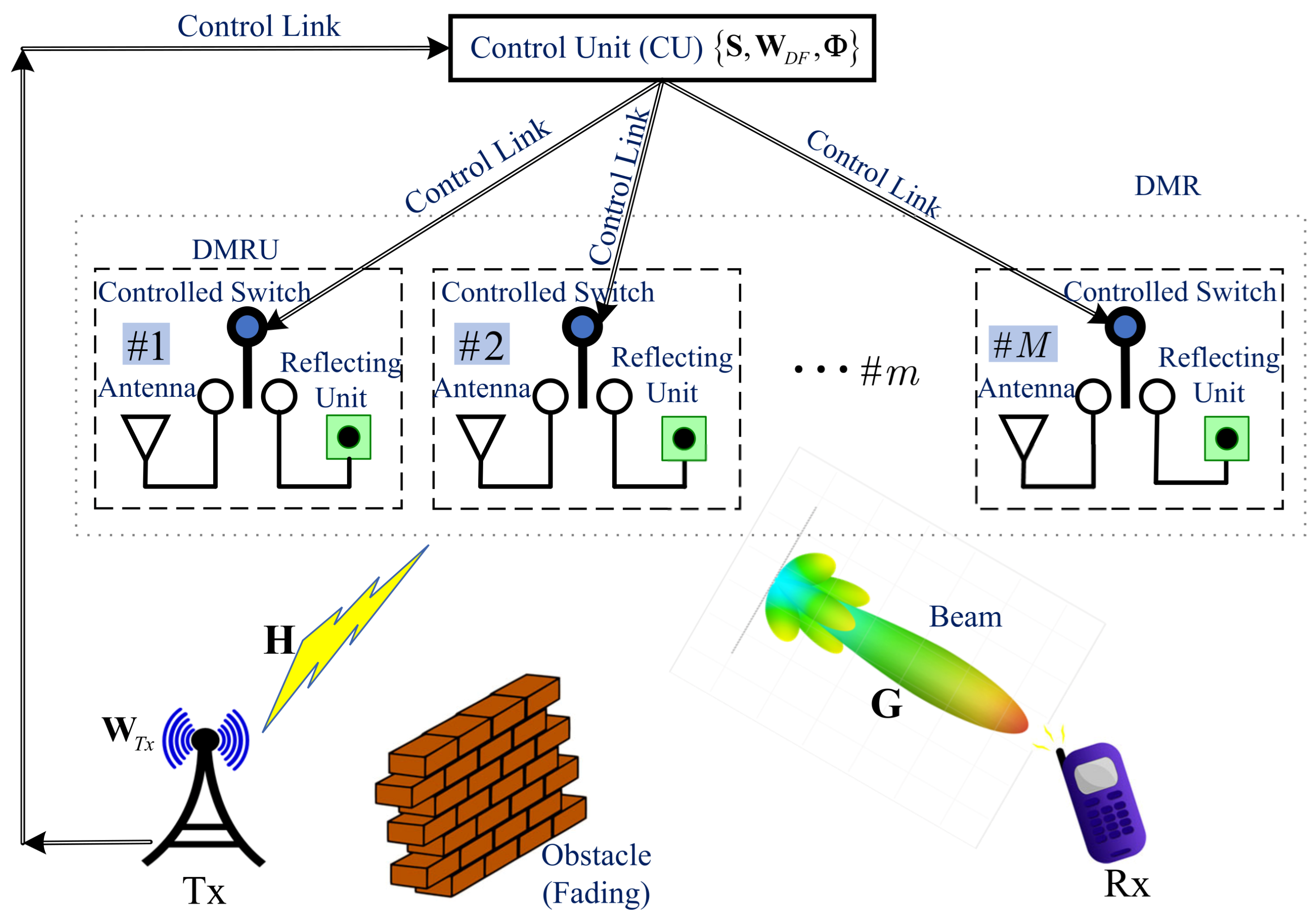
Figure 2.
Rx data rate versus for different methods and values of M.
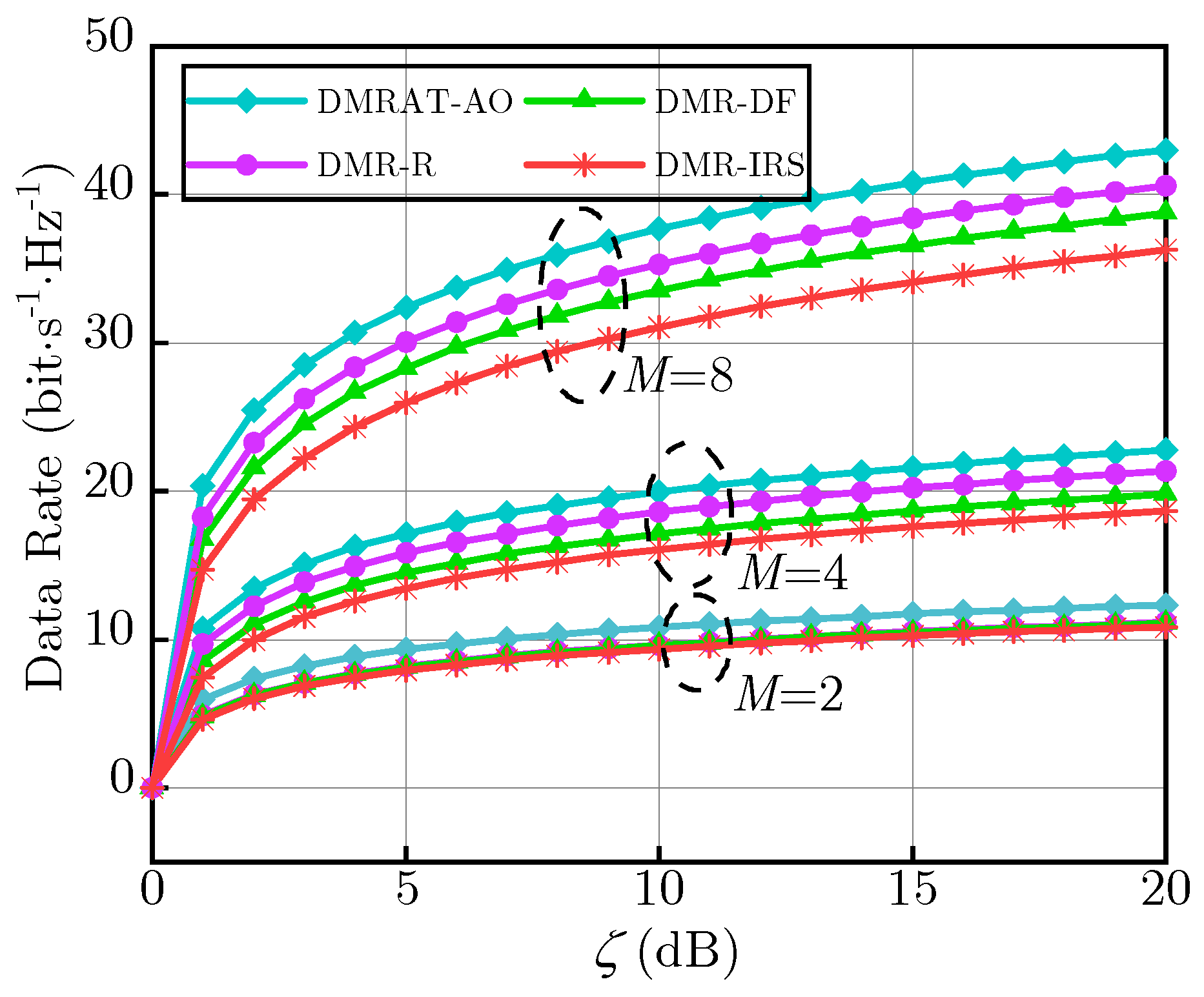
Figure 3.
Rx data rate of different methods versus the number of iterations.
Disclaimer/Publisher’s Note: The statements, opinions and data contained in all publications are solely those of the individual author(s) and contributor(s) and not of MDPI and/or the editor(s). MDPI and/or the editor(s) disclaim responsibility for any injury to people or property resulting from any ideas, methods, instructions or products referred to in the content. |
© 2025 by the authors. Licensee MDPI, Basel, Switzerland. This article is an open access article distributed under the terms and conditions of the Creative Commons Attribution (CC BY) license (http://creativecommons.org/licenses/by/4.0/).
Copyright: This open access article is published under a Creative Commons CC BY 4.0 license, which permit the free download, distribution, and reuse, provided that the author and preprint are cited in any reuse.


