
Submitted:
06 January 2026
Posted:
07 January 2026
You are already at the latest version
Abstract
Temporal reasoning is an important part of the field of time geography and spatio-temporal data science. Recent advances in qualitative temporal reasoning have developed a set of 74 relations that apply between discretized time intervals of at least two pixels each. While the identification of specific relations is important, the field of qualitative spatial and temporal reasoning relies on conceptual neighborhood graphs to address relational similarity. This similarity is paramount for generating essential decision support structures, notably reasonable aggregations of concepts into single terms and the determination of nearest neighbor queries. In this paper, conceptual neighborhoods graphs of qualitative topological changes to discretized temporal interval relations in the form of translation, isotropic scaling, and anisotropic scaling are identified using data generated through a simulation protocol. The outputs of this protocol are compared to the extant literature regarding conceptual neighborhood graphs of the Allen interval algebra, demonstrating the theoretical accuracy of the work. This work supports the development of robust spatio-temporal artificial intelligence as well as the future development of spatio-temporal query systems upon the spatio-temporal stack data architecture.
Keywords:
time geography
; qualitative reasoning
; conceptual neighborhood graph
; spatio-temporal stack
; temporal reasoning
; rasters
; topological relations
1. Introduction
Qualitative topological spatial and temporal reasoning is one of the core pieces of the research agenda of spatial information science (Figure 1) [1]. For four decades, research has been conducted to provide the theoretical tools to software developers to enhance the infrastructure of powerful spatial information systems, including formal models [2,3,4,5,6,7,8], relation sets [9,10,11,12,13,14], data structures [15,16,17,18], analysis techniques [19,20,21,22,23,24], artificial intelligence applications [25,26], and many other aspects. While the ecosystem for qualitative topological reasoning is diverse and prolific, not all of the important theoretical innovations over the past few decades have made their way into modern software. At the dawn of an age of geographic artificial intelligence [25], it is essential to integrate all available spatial and temporal reasoning insights into AI systems with the hope that that will result in interpretable, verifiable conclusions in terms that humans naturally understand. One fundamental aspect of that is of course natural language, foundational to human-computer interaction in these applications [26,27,28,29].
Geographic concepts are traditionally analyzed in static terms in typical geographic information systems, but this approach overlooks the temporal dimension that is fundamental to understanding spatial phenomena [30]. Fundamentally, geographic information science is a direct application of a broader concept: spatial information science [1,31,32,33]. Time represents an added dimension to our physical world, mathematically applied symbolically as a cross-product of an existing space and a temporal dimension [14,34] (Figure 2). On a technical level, such a concept motivates the spatio-temporal stack data structure [18], also theoretically referred to as the space-time cube. Time is fundamentally a language of change, and to fully comprehend a spatial event, in many cases temporal relations prove pivotal, yet GIS solutions minimally implement qualitative temporal reasoning directly.
To realize a spatial-temporal decision support system, it is imperative to understand the concepts behind how humans understand their environments cognitively [38]. One crucial aspect of this is found in topology [27,28,29]. Topology serves as the backbone for a large set of decisions, manifest in our spoken and written languages through prepositions [39]. Prepositions apply to both space (such as inside) and time (such as during). These terms differ only in their semantics: inside implies a physical container object, while during implies a containing temporal interval. When we consider intervals as objects, these two concepts become intuitively one and the same. These prepositions are what we might consider topological primitives, namely that they represent a mathematically explicit concept endowed in an image schemata [40]. Other prepositions behave differently, for example the spatial term along [26,28]. This term takes certain members from various topological relations (in this case disjoint, meet, overlap, coveredBy, and inside) and combines them into a specific term. Such a term is difficult for an information system to derive because of the humanistic nature of the categorization itself. Other terms such as within [41] are direct aggregates of topological primitives and are far easier to construct computationally. Terms of the latter two types benefit from aggregating similar relations, and to do that effectively, it is important to define similarity of concepts, in essence, constructing an ontology of spatial relations [42].
The conceptual neighborhood graph is a tool that has been developed to construct models of similarity among qualitative relation sets [19]. Conceptual neighborhood graphs organize the members of a qualitative relation set into a network where the nodes of the network represent relations and the edges represent a topological change under minimal units of modification called deformations. Conceptual neighborhood graphs have received a lot of attention over the last 30 years, with conceptual neighborhood graphs appearing in either the same article as the relation set (e.g., [43]) or as separate articles (e.g., [10,24]). On top of this, researchers have considered new structures of conceptual neighborhood graphs, including matrix difference neighborhoods [44], aggregates of multi-granular neighborhoods [45], intersection and union neighborhoods [46], and non-homeomorphic deformation neighborhoods [47]. While conceptual neighborhood graph research may seem archaic to some, the topic has seen a revolution with respect to the big data world and the growth of spatio-temporal artificial intelligence [25,26]. This research specifically acknowledges the variety inherent in big data, and that variety leads to a definitive need for data integration, which may need to invoke discretization neighborhoods [24,26,48] and may also need to translate topological primitives into other terms and vice versa [26,28].
The spatio-temporal stack (such as in Figure 2(a) and 2(c)) specifically creates an environment in which time is discretized [18]. To work with this reality, a set of discretized temporal relations were constructed [14]. This relation set consists of a sizable collection of 74 relations. While this may be larger than practically needed or even cognitively plausible to invoke in human thought, this result was a purely theoretical exercise: can this circumstance exist in that embedding space? To further refine that theory, conceptual neighborhood graphs provide the mechanism for determining neighboring concepts, and thus pertinent aggregations [28]. As such, it is imperative to engage in the work of determining the conceptual neighborhood graphs for this relation space. Prior work regarding spatio-temporal stack architectures did not embark on providing a query processing strategy against the structure itself that would leverage the temporal dimension [35], thus this work starts to fill a missing link. While the tools exist to ask a question such as “find all objects that overlap one another,” [41] it is a different question altogether to pose “find all objects that overlap one another which start an event where a specific object contains another specific object.” To answer this question, knowledge of both spatial [4,12] and temporal relations [9,14] are needed, and given that a human is asking the question, precisely what is meant by start [26] is also fundamental to that pursuit as well insofar as start may mean something different to different individuals without one being in error. This means that information systems to be fully human-forward need mechanisms to help users customize their query outcomes, and the most logical aggregation structures in the research are conceptual neighborhood graphs [28,29].
It is this last piece of the query (what is meant by start) where this paper provides its merit. In this paper, the conceptual neighborhood graphs for translation, anisotropic scaling, and isotropic scaling are derived from simulation data upon a pair of discretized lines embedded within . Using SQL queries upon the output data, neighboring concepts are identified based on the appropriate criteria, inducing the query through the criteria necessary to identify the appropriate change in the dataset. The outcome of such a process provides both the logic for querying a spatio-temporal data structure, but also the options a user can customize over.
The remainder of the paper is structured as follows. Section 2 introduces the basic mathematical definitions necessary for understanding the 9-intersection [4] and the 9+-intersection [49], adapted from the paper that defines the set of relations in the set [14]. Section 3 introduces the set of 74 discretized temporal relations [14]. Section 4 introduces the literature pertaining to conceptual neighborhood graphs [19]. Section 5 describes the simulation protocol and query procedure leveraged to construct the dataset (adapted from [24,48]). Section 6 presents the three conceptual neighborhood graphs for the discretized temporal relations. Section 7 analyzes the output conceptual neighborhood graphs with specific attention paid to their relationship to the neighborhood graphs of the Allen interval algebra [9,19]. Section 8 provides discussion, conclusion, and calls for future work.
2. Foundational Mathematics for the Paper
Conceptual neighborhood graphs cannot exist without the relations that serve as nodes within them. In this paper, we will be working with the set of digital interval relations in and their corresponding temporal analogs. This section will loosely follow the foundational mathematics necessary for understanding the relations from the literature [14]. The subsequent section will focus on the relations themselves, built upon the principles in this section.
The mathematics underlying qualitative topological relations in the 9-intersection family adapts concepts from point-set and algebraic topology to achieve practical usability [4,50] while maintaining mathematical rigor. This section presents the point-set topology foundations [51] that we adapt for digital lines in ℤ¹ [14]. We begin with Definitions 1-4 because they align with intuitive spatial concepts—inside, outside, and edge—making them the most accessible starting point [27].
Definition 1 (Interior): Let A be a set of points within a topological space X.
The interior of A, denoted, is the largest open set from the topological space X contained within A.
Definition 2 (Exterior): Let A be a set of points within a topological space X.
The complement of the set A, denoted by, represents the exterior of the set.
Definition 3 (Closure): Let A be a set of points within a topological space X.
The closure of the set A, denoted, is the smallest closed set from the topological space X, that contains A.
Definition 4 (Boundary): Let A be a set of points within a topological space X.
The boundary of the set A, denoted, is the set.
The interior, boundary, and exterior of an object form the vocabulary for the 9-intersection matrix, the foundational framework for spatial query systems in modern software [4]. As shown in Equation (1), the 9-intersection matrix systematically compares each of the three topological components of object A (rows) against each of the three components of object B (columns), yielding nine pairwise intersection tests.
The structure and definition of the topological components in the 9-intersection family of models depends upon the topology of the embedding space and how one defines interior, boundary, and exterior, making this family of formalisms extremely flexible for practical application in information systems. For example, in continuous space (ℝ²), a circular region’s boundary is its perimeter (a continuous curve), while in raster space (ℤ²), the boundary could have several different definitions, one of which consisting of discrete edge pixels [10,12,13,14]; despite these different interpretations, both use the same 9-intersection framework.
This flexibility supports two approaches. First, practitioners can apply formal topological methods when objects and embedding spaces have matching dimensionality (co-dimension 0), such as two-dimensional regions in two-dimensional space or one-dimensional line segments in one-dimensional space. Second, they can engineer simplified frameworks for objects in higher-dimensional spaces by treating them as their lower-dimensional equivalents. For instance, a road network (one-dimensional lines) on a two-dimensional map can be analyzed using one-dimensional interval topology, avoiding the complexity (and also limitations) of full two-dimensional spatial relations.
A common example of this phenomenon is the cartographic generalization technique for roads or rivers (converting them to linear features) on a two-dimensional map. This transformation to make intuitive topological sense applies topological understanding from the one-dimensional interval approach by ignoring one spatial dimension. This “dimensional reduction” lets analysts apply well-understood one-dimensional interval algebra instead of resorting to the role of a linear or point feature in a two-dimensional space topologically as a component of a boundary. This approach is shown in Figure 3.
The 9-intersection formalism was designed for simple objects and provides binary information (yes or no) about each intersection. Simple objects, in the most straightforward sense, have connected interiors, connected boundaries, and connected exteriors. Linear objects inherently violate this definition because their endpoints are separated from one another—you cannot travel from one endpoint to the other by staying on the boundary alone. Similarly, the line segment itself divides the exterior into two disconnected regions (before and after), as illustrated in Figure 4.
Certain objects have topological components that are inherently disconnected—where portions of the interior, boundary, or exterior are separated from one another. Linear features demonstrate this property universally: a line segment always has two separated boundary points (start and end), whether embedded in one-dimensional, two-dimensional, or higher-dimensional space. The 9⁺-intersection matrix [49] was developed to address precisely these cases where standard 9-intersection assumptions of connected components break down.
The 9⁺-intersection formalism describes diverse object types by decomposing their topological components into regular prototypical pieces. Equation (2) shows an example for two objects, each having disconnected boundaries and disconnected exteriors—a configuration that precisely characterizes intervals in one-dimensional embedding space. Although the 9⁺-intersection can express far more complex objects, this particular 5×5 structure is essential for Section 3 because digital line segments possess exactly these features: disconnected exterior regions with temporal meaning ((−<) representing “before” and (−>) representing “after”)), plus two separated boundary points (∂^< for start and ∂^> for end), each with distinct semantic significance. Figure 5 illustrates this configuration.
For the remainder of this paper, the partitions of the boundary and exterior of an object (where applicable) will follow these naming conventions.

Table 1.
Symbology lookup for Equation (2).
| Symbol | Meaning | Component Type |
|---|---|---|
| before A | left exterior of A | |
| start of A | left boundary of A | |
| during A | interior of A | |
| end of A | right boundary of A | |
| after A | right exterior of A | |
| before B | left exterior of B | |
| start of B | left boundary of B | |
| during B | interior of B | |
| end of B | right boundary of B | |
| after B | right exterior of B |
3. Discretized Temporal Relations
Temporal relations represent some of the earliest (and also most recent) work within the geographic information science community. As with the history of most formalisms for object relation sets, the vectorized sets came first, then followed by discretized versions (e.g., [9] and [14], [10,12,50], and [13,43]).
The Allen interval algebra serves as the foundation for studies of temporal relations in an abstract sense [9]. Allen’s work specified intervals by their starting and ending points in . Allen explored the 25 possible sequences of boundary points and determined that 13 of those relations were realizable given basic constraints about boundary points simultaneously occupying either the starting or ending point of the other boundary (eliminating two candidates) and that the ending point of an interval must naturally come after its starting point (eliminating a further ten candidates). The resulting relations are shown in Table 2.
The relations in Table 2 have a definitive relationship to one another. Relations such as before and after are temporally inverted relations. These relations consider the mirror image of the relation. In continuous spaces, this is related to converse relations: if a is before b, then it is directly implied that b is after a. This set of relations is comprised of five temporally inverted pairs and an additional three relations that are self-inverted (or temporally symmetric) (equal, inside, contains), as shown in Table 3 [9].
The Allen interval algebra became the springboard by which to consider minimum bounding rectangle relations [6], direction relations [7,8,53], but also (more importantly for this paper) discretized temporal intervals [14]. To maintain starting and ending points that are part of the accessible space, the digital Jordan curve [3] was chosen to represent these intervals in . Given this definition, it is possible for an object to consist of only boundary, a similar result to discretized region-region relations in [12]. With the assertion that an interval object must have distinct starting and ending points, a series of constraints were applied in a constraint sieve to isolate verifiable relations between intervals in based on their 9-intersection and 9+-intersection symbols [14]. The constraint sieve identified 34 relations (with an additional eight relations present if considering touching relations) in the 9-intersection are shown in Table 4 [10,14].
As seen in Table 3, the relations in Table 4 have temporal analogs, just as their continuous counterparts do. They can be constructed by considering a mirror image of the space. Symbolically, this means that the 9+-intersection is transformed in the following manner:
This will not change the 9-intersection relation, and it furthermore constructs distinct relations for 32 of the 42 non-ordered line-line relations, creating a total of 74 9+-intersection relations [14]. Theorem 1 describes why the 9-intersection relation is equivalent for temporally ordered relations. Theorem 2 addresses that there are exactly two configurations for outcomes of Equation (3).
Definition 5.
A relation is called temporally symmetric if the relation is unchanged by exchanging its before and after components in the 9+-intersection for objects A and B as expressed in Equation (3), namely . Otherwise, the relation is called temporally invertible.
Theorem 1.
Consider the matrix transformation t in Equation (3). The matrix transformation does not influence the 9-intersection matrix.
Proof.
The 9-intersection matrix (Equation (1)) can be derived from the 9+-intersection matrix (Equation (2)) by identifying if there is a non-empty intersection in any cell of the 9+-intersecfion that would map back to the cells in the 9-intersection. Based on the configuration in Equation (2), the corresponding cell mapping between Equation (2) and Equation (1) is shown in Equation (4):
The transformation in Equation (3) represents a horizontal and then vertical flip of the 9+-intersection in Equation (2), effectively rotating the matrix 180 degrees. When this is accomplished, the cell holds a very similar structural position to what it held before, just in a mirrored position within the matrix. Since Equation (4) is both vertically and horizontally symmetric, any transformation that flips the original matrix horizontally or vertically will be maintained under this transformation, and this is precisely what Equation (3) does twice in succession. Exchanging the before components of A within the relation for the after components of A results in a vertical flip; exchanging the before components of B with the after components of B results in a horizontal flip.
Theorem 2.
Consider the matrix transformation from Equation (3).is its own inverse.
Proof.
Temporally symmetric relations have the function t as an identity function. If we consider what the function itself represents as an action, it is intuitive that Equation (3) is its own inverse. As discussed in Theorem 1, Equation (3) represents a horizontal flip followed by a vertical flip of the input matrix m, with each flip representing the exchange of the before and after components of objects A and B. For a function to be its own inverse, reapplying the function must result in the original input. Flipping the values back again reverts both objects to their original configuration. Since the 9+-intersection is unique for a drawn scenario, .
Theorem 2 dictates that a relation either is temporally symmetric, or it is directly paired with another relation in the set as a temporal inverse. Because m exists, t(m) must also fit the same criteria from the constraint sieve. Since t(m) is its own inverse, Theorem 2 dictates that the chain stops there. The resulting relations from the temporal folding are shown in Table 5.
Table 5 shows each pair of relations as suggested by Theorem 2. It is clear that there is an organizing principle connecting the relations together. If a relation is converse, red relations become yellow, while blue and green remain blue and green. If a relation is temporally inverted, its color remains the same. This set of relational images, identified by 9+-intersection matrices [49], forms the vocabulary for the remainder of this paper. Relations in subsequent sections of the paper will be identified based on their names from Table 4 and Table 5 as appropriate.
4. Conceptual Neighborhood Graphs
Relation sets (such as in Section 3) form the vocabulary of qualitative topological reasoning. These features become critical features of human-centric query systems [43,54]. The vocabulary of a relation set, however, is not enough. There is an implicit set of relationships between the relations themselves insofar as when an object is deformed in a certain way, there are predictable behaviors exhibited in the configurations of those relations that describe the next configuration(s). The research outcome that describes this deformational pathway is called the conceptual neighborhood graph [19].
Freksa [19] first utilized the conceptual neighborhood graph principle to explain the relationships between the Allen interval algebra relations under three specific conditions (Figure 6):
- anisotropic scaling, namely one of the objects has a boundary point moved, while the other three boundary points in the scene remain fixed (called the A neighborhood),
- translation, namely one of the objects moves without changing its duration while the other is unaltered (called the B neighborhood), and
- isotropic scaling, namely one of the objects grows (or shrinks) the same amount at each boundary point while the other remains unaltered (called the C neighborhood).
In essence, whenever a change in relation is encountered between the prior state and the modified state as a function of a particular deformation to an object, an edge is constructed in the conceptual neighborhood graph. The three conceptual neighborhood graphs are shown in Figure 7.
It is important to recognize that these three distinct conceptual neighborhood graphs are necessarily different from one another. The differences in the conceptual neighborhood graphs are the direct result of the type of allowable deformation. To highlight what is occurring, consider the relation equal. If two objects that start as equal have one of the four boundary points move (without loss of generality, one of A’s boundary points), the direction of movement will change the relation in each case to something different. One pair of boundary points will however remain fused together. This particular deformation changes equal to either starts, started by, finishes, or finished by depending upon which boundary point is moved. This is shown in Figure 7(a). If that same equal configuration undergoes translation, if object A moves left, it now overlaps object B. Similarly, if it moves right, it now is overlapped by object B. This is shown in Figure 7(b). Finally, if an equal object grows in both directions, it will now contain object B. Similarly, if it shrinks, it will now be during object B. This is shown in Figure 7(c). As such, the structure of the specific conceptual neighborhood graph is fully dependent upon the type of deformation(s) allowed. An edge exists if and only if under that particular deformation (or deformations in a multi-option scenario [46]), the specific relation can be converted to the connected relation without going through an intermediary step first.
Several other ways of envisioning conceptual neighborhood graphs have been found in the literature over the last 30 years. Examples of these innovations include accounting for changes to the topological structure of an object by adding holes or separations [47], least matrix difference [44], intersections and unions of conceptual neighborhood graphs to reflect various purposes [46], mixed granularity neighborhoods [45], discretization neighborhoods [24,48], and association rules mining neighborhood graphs [24,48]. Independent of the type of conceptual neighborhood graph, rules exist to define what constitutes an edge in the graph.
5. Simulation Protocol
Recent advances in conceptual neighborhood graphs involve discretized relations. Hall and colleagues [24,48] constructed conceptual neighborhood graphs in using a simulation protocol that involved fixing a discretized object in of a fixed size and systematically moving another object of fixed size pixel by pixel throughout an embedding grid. After the configuration was finished, the embedding was reset, with one of the objects changing its dimensions, and the process continued. This process continued until all possible configurations were completed between discretized rectangles. This simulation protocol is summarized in Figure 8 as applied to a subspace of large enough to bound a particular object on either side of another ground object A.
. The only difference in the approaches is that the second dimension from the original protocol is not considered.
The simulation protocol requires several parameters to ensure complete relational coverage while limiting computational overhead. Based on prior research [24,48], we set the maximum interval size to s = 10 pixels, as no new relations emerge between two-dimensional raster objects beyond this size. This finding transfers to one-dimensional intervals, allowing us to constrain the search space.
The embedding array size (a = 32) follows from the formula:
This ensures sufficient space for: (1) a maximum-size interval for object A, (2) a maximum-size interval for object B, and (3) enough exterior space on both sides to represent the before and after relations without boundary contact (e.g., B1 and A1 from Table 5).
The fixed object position (p = 12) is determined by:
This placement allows a moving interval to occupy any position from fully before the fixed interval (including a gap) to fully after it, covering all spatial configurations including the relational extremes of before and after.
To uniquely identify each intersection component, we encode object A as integer values (0 for exterior, 1 for boundary, 2 for interior) and object B as decimal values (0.0 for exterior, 0.1 for boundary, 0.2 for interior). Their sum produces a unique signature for each of the nine 9-intersection components, following the encoding method demonstrated in [24,48].
All other implementation details—such as the iteration order over positions and interval lengths—are arbitrary provided the simulation achieves complete coverage of the four-dimensional parameter space ⟨length₁, length₂, position₁, position₂⟩.
This dataset records the duration of each object, the position of the moving object, and the topological relation between the two interval objects. With this data, an SQLite database was queried to extract relations symbolic of each relevant homeomorphic deformation based on information in the rows of the dataset, consistent with Hall and colleagues [24].
Similar to the prior protocol, when defining each conceptual neighborhood graph, two possible types of neighbors could exist: persistent neighbors and coincidental neighbors. Persistent neighbors are neighbors such that when both relations can exist at a particular pair of durations of their constituent objects, they are always neighbors. A good example of this would be relations such as before and meets from the Allen interval algebra. Coincidental neighbors are just that: they happen by chance, but they are not always neighbors under all configurations where those relations are available. An example of that phenomenon would be overlapMeet and overlapCovers from the region-region relations in [24,48]. These are only neighbors where the size of at least one of the objects is insufficient to support overlap, the appropriate intermediary relation that would be expected from continuous space [43,55]. We are interested predominantly in persistent neighbors in this paper.
Each homeomorphic deformation type (Section 4) produces a distinct signature in the simulation data based on how position and length change between consecutive states. These signatures enable systematic extraction of conceptual neighbors through SQL queries. These signatures are as follows:
- ○
-
Translation- moves an interval without changing its size:
- ▪
- Position changes by ±1
- ▪
- Length remains constant
- ○
-
Isotropic scaling -expands or contracts the interval symmetrically from its center:
- ▪
- Growth: length increases by 2 (one pixel each side), position decreases by 1 (center shifts left)
- ▪
- Shrinkage: length decreases by 2 (one pixel each side), position increases by (center shifts right)
- ○
-
Anisotropic scaling - extends or contracts the interval from one endpoint:
- ▪
- Left extension: length +1, position -1 (start point moves left)
- ▪
- Right extension: length +1, position unchanged (end point moves right)
- ▪
- Left contraction: length -1, position +1 (start point moves right)
- ▪
- Right contraction: length -1, position unchanged (end point moves left)
Each of these deformation patterns translate directly into SQL join conditions. Equations (7)–(9) show queries that identify conceptual neighbors by matching these signatures in the simulation data. Translation is shown in Equation (7); isotropic scaling is shown in Equation 8; anisotropic scaling is shown in Equation (9).
SELECT S1.Relation, S2.Relation
FROM Simulation AS S1 INNER JOIN Simulation AS S2
ON ((S1.X=S2.X+1 OR S1.X = S2.X-1) AND S1.L1=S2.L1 AND S1.L2=S2.L2)
WHERE S1.Relation != S2.Relation (7)
SELECT S1.Relation, S2.Relation
FROM Simulation AS S1 INNER JOIN Simulation AS S2
ON ((S1.X=S2.X+1 AND S1.L1=S2.L1-2 AND S1.L2=S2.L2) OR (S1.X=S2.X-1 AND S2.L1+2 AND S1.L2=S2.L2) OR (S1.L2=S2.L2-2 AND S1.X=S2.X-1) OR (S1.L2=S2.L2+2 AND S1.X=S2.X+1))
WHERE S1.Relation != S2.Relation (8)
SELECT S1.Relation, S2.Relation
FROM Simulation AS S1 INNER JOIN Simulation AS S2
ON ((S1.X=S2.X AND S1.L1=S2.L1+1 AND S1.L2=S2.L2) OR (S1.X=S2.X AND S1.L1=S2.L1-1 AND S1.L2=S2.L2) OR (S1.X=S2.X-1 AND S1.L1=S2.L1+1 and S1.L2=S2.L2) OR (S1.X=S2.X+1 AND S1.L1=S2.L1-1 AND S1.L2=S2.L2) OR (S1.L2=S2.L2-1 AND S1.L1=S2.L1 AND S1.X=S2.X) OR (S1.L1=S2.L1+1 AND S1.L1=S2.L1 AND S1.X=S2.X) OR (S1.L2=S2.L2+1 AND S1.L1=S2.L1 AND S1.X=S2.X+1) OR (S1.L2=S2.L2-1 AND S1.L1=S2.L1 AND S1.X=S2.X-1)
WHERE S1.Relation != S2.Relation (9)
Although generated through simulation, this dataset is theoretically complete and fully representative due to the finite nature of discrete spaces. In discrete embeddings, the set of possible relations reaches closure—no new relations emerge beyond a certain object size, and consequently, no new conceptual neighbor pairs emerge either. This closure property eliminates the need for formal algebraic proofs, though such proofs remain theoretically feasible. The structural constraints of intervals in one-dimensional discrete space severely limit configurational possibilities, making exhaustive enumeration through simulation both practical and sufficient.
6. Results
The SQL queries from Section 5 create a set of records that can be visualized as graphical outputs. Section 6 shows the outcomes of these graphs for both the 9-intersection relations from Table 4 and the 9+-intersection relations from Table 5 [14]. Each graphic will be broken into types of relations by symbology approaches that have an impact on the analysis (e.g., 9-intersection relation families as color; presence of an interior as shape). The results for translation, isotropic scaling, and anisotropic scaling are shown in Figure 9, Figure 10 and Figure 11 and Table 6, Table 7 and Table 8. Interactive 3-D representations of the figures in this section can be accessed here.
The translation conceptual neighborhood graph specifically is influenced by the size of the intervals that take part in the relation, creating a disconnected graph, a unique feature amongst existing conceptual neighborhood graphs in the literature. This is clearly visible in Figure 9. Because translation does not alter the interval objects as a result of the deformation, any relations that are size dependent or have no interior retain that feature and thus are exclusionary to connection to other relations that do not fit those same parameters by default. The two graphs on the top and bottom of Figure 6 are mirror images of each other as they are composed of converse scenarios (the triangular symbology relations have an A without an interior, while the diamond symbology relations have a B without an interior). This represents an effective test of the simulation protocol because the size dependent relations remain disconnected from one another. Similarly, the relations with no interior for either A or B (left-center, square symbology) form their own specialized group. Additionally, there are touch relations that are not distinguishable by the 9-intersection, but hold a specialized transitional meaning that has been recognized in numerous other studies [10,12,13,14]. These relations sit between relations disjoint/inside/contains and their corresponding boundary sharing relations meet/coveredBy/covers. The main part of the graph (relations where both digital intervals have interiors) is completely symmetric with one size restricted relation branching from meet. Unique to the conceptual neighborhood graphs in this study, it is the only one which is planar. Table 6 shows the fundamental symmetry of the graph through the basic rule that the converse relation must relate to the converses of those relations that the original relation relates to. The most connected relation is M1 with a degree of 5.
The isotropic scaling conceptual neighborhood graph is exactly symmetric, as shown directly in Table 7. It also exhibits the converse behavior expected. In terms of representing the graph in Figure 10, only one relation is displaced and that is to make sure that connections remain visible. The graph is clearly not planar. Unlike Figure 9, the relations that come from particular symbology groups in the image are not interconnected (other than the circular symbology relations and some triangular symbology and diamond symbology relations, but not all). This is an important assertion that mirrors how discretized relations have long been seen: spend time developing infrastructure around the relations comprised of larger objects because they are more commonly found, a reality that constructed multiple pieces in the literature about discretized region-region relations [10,12,13]. The circular symbology relations form the bedrock of this graph. Once these relations get sufficiently small, they connect to triangular symbology and diamond symbology relations, and then those connect to square symbology relations. As such, the square symbology relations are isolated from one another. Square symbology relations transition into triangular relations as B grows and to diamond symbology relations as A grows. Triangular symbology relations transition to circular symbology relations as B grows and connect to triangular symbology relations as A grows. Diamond symbology relations transition to circular symbology relations as A grows and connect to diamond symbology relations as B grows. The predictability of the transition between symbology shape families in this graph provides further evidence of the accuracy of the simulations. The most connected relations in this graph are M1 and O8, both with degree 6.
The anisotropic scaling conceptual neighborhood graph shows a similar symbology shape transfer pattern to isotropic scaling. Anisotropic scaling is a much more convoluted pattern due to there being four pulling directions (as opposed to two), but also maintains symmetry, consistent with isotropic scaling. Similar to isotropic scaling, this graph is also non-planar. Similar to the other graphs, it is plainly converse fulfilling and symmetric. The most connected relation in this graph is M1 with a degree of 8.
To get to temporal relations, we can simply append the graphs together across temporally symmetric relations. Temporally symmetric relations (as discussed in Definition 5) do not differ when the before components of the relation are exchanged with the after components of the relation. The temporally symmetric relations are E1, E2, C1, C2, C4, C5, I1, I2, I4, and I5. In each case, the relation itself does not change if one considers a mirror image of that relation. In the other cases, a relation from the 9-intersection has two forms in the 9+-intersection: one corresponding to the lefthand side (the before/starts group) and one corresponding to the righthand side (the after/finishes group). All further analyses regarding properties of the graphs themselves mirror those from Figure 9, Figure 10 and Figure 11. These graphs are shown in Figure 12, Figure 13 and Figure 14.
7. Comparison of Discretized Temporal Conceptual Neighborhood Graphs to Continuous Temporal Conceptual Neighborhood Graphs
Dube [14] demonstrated that the discretized temporal interval relations fit into categories that reflect a corresponding Allen interval relation [9]. This assertion motivated the structure of Table 5. As such, it is hypothesized that the conceptual neighbors of each relation within a specified conceptual neighborhood graph are either of the same Allen family (such as in Table 5), or neighbor a relation in an Allen family that is a conceptual neighbor in the corresponding conceptual neighborhood graphs of the Allen interval relations (such as in Figure 7). Such a result would be further evidence of the simulation method working. Hall and Dube [24] demonstrated the discretized region-region relation conceptual neighborhood graphs followed this exact behavior. Given that these objects are of co-dimension 0 to their embedding space (just as in the region-region case), the same behavior is expected. The outcomes are shown in Table 9, Table 10 and Table 11.
The translation conceptual neighborhood graph behaves exactly as expected. Each type of relation attaches appropriately to the corresponding relations in the B neighborhood. This is most easily observed around equal: equal attaches only to the overlap group and not to the coveredBy, covers, inside, or contains groups. Similarly, contains, inside, and disjoint do not directly connect to overlap, thus forming the explicit structure in Figure 7(b). The relations without an interior for one or more of the objects induce connections that bypass relations that cannot exist in those groups, for example equal, coveredBy, and covers connecting to meet because overlap is not available.
Table 10 shows a behavior that at first does not seem to fit the predicted behavior: two relations from the coveredBy family (CB2, CB4) connect to a relations from the covers family (CV2, CV4), which violates the structure of Freksa’s C-neighborhood (Figure 7(c)). This additional connection, however, is an important one to really get a feel for what is happening with discretized relations as compared to continuous relations. Unlike the dense intervals in continuous space, objects have to grow in chunks. This is made most plain when we consider the relations that have an object with no interior that then exhausts the interior of another object with one of its boundaries (e.g., CB4 and CV4). As the object without an interior grows, it will encounter relations CV2 and CB2 respectively. This is specifically because of the relative size. CB2 and CV2 also connect to one another for the exact same reason. While this violates Freksa’s C-neighborhood, this is not the first time such a result has been seen in discretized relations. In fact, the region-region relations exhibit this same exact behavior [24,48] as a function of relative size, a concept that is irrelevant in continuous embedding spaces. The reason that the result does not appear functionally within the group is the presence of an intermediary relation overlapFully. This new feature in the conceptual neighborhood graph, however, follows the lateral pattern exhibited in the C-neighborhood between inside, equal, and contains.
Anisotropic scaling is far more predictable and exhibits the behaviors expected from Freksa’s A-neighborhood (Figure 7(a)). This is more predictable than isotropic behavior because only one pixel changes its classification in each change, whereas isotropic scaling must examine the changes to two pixels. This result is suggestive of the matrix-difference neighborhoods suggested in prior research [44].
When we aggregate the neighborhoods across the blue relations in Table 9, Table 10 and Table 11, the aggregated conceptual neighborhood graphs are shown in Figure 15. Other than the connection between coveredBy and covers in Figure 15(c), there are no differences in these conceptual neighborhood graphs from their continuous counterparts.
Because the temporal versions of these relations are inverse copies, the graphs can be glued together over the symmetric relations inside, equal, and contains.
8. Discussion, Conclusions, and Future Work
In this paper, the set of discretized temporal relations [14] were placed into three distinct conceptual neighborhood graphs, each representing a different homeomorphic deformation of a single discretized temporal interval. It was shown that the discretized temporal interval relations organized into these neighborhood graphs in a predictable manner from the corresponding continuous temporal interval relations [9,19], a behavior similar to the discretized region-region relations [10,24].
On its surface, this work appears as a “replication of a classic” study (in this case, the work of Freksa [19]). By working with discretized intervals (temporal or otherwise), though a classical method is recreated, there are numerous advantages that access to conceptual neighborhood graphs provide within this setting [26]. While these types of constructions have long been available for continuous objects, they have only more recently been studied for their discretized cousins [24], and the deformations do not necessarily behave as subtly in all cases as they do in the continuous embedding spaces. On a relational level, discretized intervals (and thus relations between them) [14] are necessarily approximations of their real-world counterparts, resulting in an increase in the volume of relations available in these relational dictionaries. This increase in volume allows for more surgical precision in choosing datapoints of interest in applications. A simple example of this can be seen by using the size constraints of objects. Not all relations are available between objects of particular sizes, as seen easily in Figure 9 and Figure 12 discussing translation. Knowing that restriction provides much more nuance in their applications than Freksa’s work suggests in the continuous domain where such concerns are largely irrelevant due to the denseness of continuous embedding spaces. As shown in prior research, choosing a configuration of object sizes influences the structure of the conceptual neighborhood graph, resulting in relations that are always neighbors and relations that are neighbors only within a particular context and would not be neighbors otherwise [24,48]. Different applications of the same idea create filtration and aggregation opportunities that are customizable to their context [26], be it through mathematical means or via user selection, presumably motivated by the conceptual neighborhood graphs in this work as concepts in human thought have been shown to have connected signatures in these graphs [28,29,57].
The results of this work provide a critical piece of infrastructure for spatio-temporal knowledge discovery. Knowledge discovery predominantly requires the detection of events. This work relates to the detection of spatio-temporal events. To determine events, it is imperative to be able to map human language onto computational data sources as ultimately humans will ask the questions or an artificially intelligent agent will need to translate the results of its operations back into human language itself [25,26,27,28,29,40,43,56]. While the relations themselves represent the primitive space for that mapping, they do not represent fully the construction of human language which might abstract away less critical details that are unnecessary for the circumstance (such as the within operator in a modern GIS). Conceptual neighborhood graphs provide the easiest possible way to model that behavior because humans naturally group relations that share fundamental similarity. An easy example of this is shown in Figure 16. Dube and Egenhofer [28] demonstrated that this concept is not only manifest in reasonably topological spatial terms, but also showed that those terms held specific mathematical properties within the conceptual neighborhood graphs themselves, specifically convexity. Convex subgraphs maintain all possible shortest paths between their vertices from within the graph overall. Most qualitative spatial reasoning work has focused on conquering the layers of the spatio-temporal stack; this work focuses on conquering the stacking dimension. As such, one direct contribution of this paper is the skeleton for the construction of human-centric queries that are either a specific symbol or an aggregate of connected symbols. The conceptual neighborhood graphs (or their unions and/or intersections) represent that skeleton. Human-subjects testing would be required to create specific aggregates within software that are most commonly used. Without human-subjects testing, software interfaces could be developed that give the user flexibility in choosing the appropriate relation terms to be aggregated, be it through consistent information in their 9-intersection or 9+-intersection signatures (e.g., [41]), or via specific user choice. The added benefit of a choice-based approach is that users can specifically choose a more nuanced view of a phenomenon. While this approach seemingly violates the premise of Occam’s razor, the computational tool is not bound by this human construct implicitly. One challenge in current GIS tools is specifically that the “select by location” infrastructure does not provide avenues for custom queries in its user interface, relegating this to more advanced programming language applications such as the st_relates function in the sf library [58] or in GeoPandas [59]. None of the available spatial libraries in available programming languages possess infrastructure for digital topological relations of any kind (be they spatial or temporal), let alone aggregates of them motivated by conceptual neighborhood graphs. Work is currently ongoing to integrate these types of relations into spatio-temporal libraries such as SpaceTime [60], the first step to having practical tools operable in software that leverage corresponding conceptual neighborhood graph insights directly.
Not only is this concept fundamental to defining terms; it is also a matter of pragmatism in our data forward world with respect to data filtration [26]. Decision support systems function differently than do information systems. Information systems determine what fits sufficient criteria only; decision support systems are interested in ranking solutions. The conceptual neighborhood graph provides the framework by which a decision support system can support “next best” results. Furthermore, a conceptual neighborhood graph architecture (if endowed in the decision support system’s query logic or within the programming of an artificially intelligent geospatial agent) allows for a user to specify the exact nature of the specificity of their query. Because discretized representations of data are fundamentally uncertain with respect to a continuous space that they in effect model, it is possible that particular edges of the conceptual neighborhood graph may lead to relevant neighbors in a contextual application, while others would not. Without conceptual neighborhood graphs as a guiding paradigm, this problem is not cognitively simple, requiring humans to recognize the variability within the conceptual neighborhood graph by their own devices; with a conceptual neighborhood graph, this process has simple guideposts to direct the refinement of the query itself that can be coached by an artificially intelligent agent or by basic cascading logic within software. For example, if a user deems inside to be their prerogative in a query, the system can ask in return about the conceptual neighbors of inside and give the user the opportunity to include or exclude them. This process can continue until the user adds no additional search terms. These innovations lead to smarter data systems overall.
While there are many families of conceptual neighborhood graphs that have been developed (almost as numerous as relation sets themselves), there is still much work to be done. While most conceptual neighborhood graphs focus on homeomorphic deformations, there are other very crucial transformations that fundamentally alter objects structurally. Most notably for temporal intervals is the concept of the conversion between discretization and vectorization. This paper demonstrates the linkage between these dimensions in Section 7. The future work that this leads to is a conceptual neighborhood graph that fundamentally links these concepts, effectively a layered conceptual neighborhood graph. An example of this concept applied to direction reasoning is shown in Figure 17, where the only difference between the layers is whether or not the point itself (the circle in the center of each symbol) is part of the direction field or not [53]. This work has been suggested both here and in its region-region counterpart [24].
To fully realize this line of research, two fundamental concepts remain. The first is an appropriate definition of lines in and their corresponding relation sets and conceptual neighborhood graphs. The second is to consider yet another type of conceptual neighborhood graph: a generalization neighborhood. Cartographic generalization is a critical component of geographic information science [61,62,63,64]. In our big data world, we must cope with the large variety of data representations. To appropriately do that, we must come to a fundamental understanding and synergy of continuous and discretized spaces. By considering both a discretization/vectorization and cartographic generalization neighborhood, we will be able to leverage more data resources toward our worthy tasks, whatever they are [26]. For example, consider the term outside. There are corresponding versions of separated in all relational sets, which is not surprising because it is one of the core parts of the Natural Semantic Metalanguage [65]. Though objects may not structurally be the same, the same root image schemata [40] is involved in this characterization. More importantly, because we generalize objects on the fly [66,67], two representations may actually be discussing the same object with that object existing in different cartographic forms, and thus on their own existing in one conceptual neighborhood graph that is perhaps different than the one in the other representation. Both of these scenarios demonstrate the necessity to understand this particular concept of relational similarity across different types of deformations that have not been fully explored. The basic infrastructure to consider a generalization neighborhood exists within continuous spaces as all of the types of relations between simple objects have conceptual neighborhood graphs established [56,57,68], but it does not exist within discretized spaces yet due to the definition of lines in being missing.
Of course, the overall goal for all of this research agenda is the creation of a fully endowed qualitative spatio-temporal decision support system [69] and eventually geospatial AI with similar capacity [25,26]. To fully realize this, it is more than just a technical exercise of data structures and theoretical reasoning formalisms; this process involves the intrinsic knowledge of how humans interact with a system and making that usable on those terms, most notably their cognitive structures and their ability to strategically problem solve [29]. The qualitative spatial reasoning and spatial cognition community need to come together to figure out the structure appropriate for a query language designed with these principles in mind and work in concert with the software engineering and user experience design communities to construct software and programming languages that can embed those insights. Theoretical formalisms and data structures guide this process, but there is much work with human subjects to be done to get the linguistic concepts correct, a basic concept that made a language like SQL successful [70].
Author Contributions
Conceptualization, Matthew P. Dube and Brendan P. Hall; methodology, Matthew P. Dube and Brendan P. Hall; software, Brendan P. Hall; validation, Matthew P. Dube and Brendan P. Hall; formal analysis, Matthew P. Dube; investigation, Matthew P. Dube; resources, Matthew P. Dube and Brendan P. Hall; data curation, Brendan P. Hall; writing—original draft preparation, Matthew P. Dube; writing—review & editing, Matthew P. Dube and Brendan P. Hall; visualization, Matthew P. Dube and Brendan P. Hall; supervision, Matthew P. Dube; project administration, Matthew P. Dube; funding acquisition, Matthew P. Dube. All authors have read and agreed to the published version of the manuscript.
Funding
Matthew P. Dube was funded by the US National Science Foundation, grant numbers 2019740 and 2218063.
Conflicts of Interest
Author Brendan P. Hall was employed by the James W. Sewall Company. The remaining authors declare that the research was conducted in the absence of any commercial or financial relationships that could be construed as a potential conflict of interest.
References
- Claramunt, C.; Dube, M.P. A brief review of the evolution of GIScience since the NCGIA Research Agenda initiatives. Journal of Spatial Information Science 2023, 26, 137–150. [Google Scholar] [CrossRef]
- Clarke, B. A calculus of individuals based on “connection”. Notre Dame Journal of Formal Logic 1981, 22(3), 204–218. [Google Scholar] [CrossRef]
- Vince, A.; Little, C.H. Discrete Jordan curve theorems. Journal of Combinatorial Theory, Series B 1989, 47(3), 251–261. [Google Scholar] [CrossRef]
- Egenhofer, M.J.; Herring, J.R. Categorizing binary topological relations between regions, lines, and points in geographic databases. NCGIA Technical Report, 1990.
- Randell, D.A.; Cui, Z.; Cohn, A.G. A spatial logic based on regions and connection. In Principles of Knowledge Representation and Reasoning; Nebel, B., Rich, C., Swartout, W.R., Eds.; Morgan Kaufmann Publishers: San Francisco, CA, USA, 1992; pp. 165–176. [Google Scholar]
- Papadias, D.; Sellis, T.; Theodoridis, Y.; Egenhofer, M.J. Topological relations in the world of minimum bounding rectangles: a study with R-trees. In Proceedings of the 1995 ACM SIGMOD International Conference on Management of Data; Carey, M., Schneider, D., Eds.; ACM Press: Washington, D.C., USA, 1995; pp. 92–103. [Google Scholar]
- Goyal, R. Similarity assessment for cardinal directions between extended spatial objects. Doctoral Dissertation, University of Maine, Orono, ME, United States, 2000. [Google Scholar]
- Dube, M.P. Topological augmentation: a step forward for qualitative partition reasoning. Journal of Spatial Information Science 2017, 14(1), 1–29. [Google Scholar] [CrossRef]
- Allen, J.F. Maintaining knowledge about temporal intervals. Communications of the ACM 1983, 26(11), 832-843. [CrossRef]
- Egenhofer, M.J.; Sharma, J. Topological relations between in regions in and . In International Symposium on Spatial Databases; Abel, D.J., Ooi, B.C., Eds. Springer-Verlag: Berlin, Germany, 1993; pp. 316-336.
- Balbiani, P.; Osmani, A. A model for reasoning about topological relations between cyclic intervals. In Principles of Knowledge Representation and Reasoning; Cohn, A.G., Giunchiglia, F., Selman, B., Eds.; Morgan Kaufmann Publishers: San Francisco, CA, USA, 2000; pp. 378–385. [Google Scholar]
- Dube, M.P.; Egenhofer, M.J.; Barrett, J.V.; Simpson, N.J. Beyond the digital Jordan curve: unconstrained simple pixel-based raster relations. Journal of Computer Languages 2019, 54, 100906. [Google Scholar] [CrossRef]
- Dube, M.P.; Egenhofer, M.J. Binary topological relations on the digital sphere. International Journal of Approximate Reasoning 2020, 116, 62–84. [Google Scholar] [CrossRef]
- Dube, M.P. Digital relations in : discretized time and rasterized lines. International Journal of Geo-information 2025, 14(9), 327. [CrossRef]
- Robertson, C.; Chaudhuri, C.; Hojati, M.; Roberts, S. An integrated environmental analytics system (IDEAS) based on a DGGS. ISPRS Journal of Photogrammetry and Remote Sensing 2020, 162, 214–228. [Google Scholar] [CrossRef]
- Environmental Systems Research Institute. ESRI Shapefile Technical Description. ESRI Technical Report, 1998.
- Winter, S. Topological relations between discrete regions. In International Symposium on Spatial Databases; Egenhofer, M.J., Herring, J.R., Eds.; Springer-Verlag: Berlin, Germany, 1995; pp. 310–327. [Google Scholar]
- Yuan, M. Use of a three-domain representation to enhance GIS support for complex spatiotemporal queries. Transactions in GIS 1999, 3(2), 137–159. [Google Scholar] [CrossRef]
- Freksa, C. Temporal reasoning based on semi-intervals. Artificial Intelligence 1992, 54(1-2), 199–227. [Google Scholar] [CrossRef]
- Egenhofer, M.J. Deriving the composition of binary topological relations. Journal of Visual Languages and Computing 1994, 5(2), 133–149. [Google Scholar] [CrossRef]
- Duntsch, I.; Orlowska, E. Discrete dualities for some algebras with relations. Journal of Logical and Algebraic Methods in Programming 2014, 83(2), 169–179. [Google Scholar] [CrossRef]
- Hornsby, K.S.; Li, N. Conceptual framework for modeling dynamic paths from natural language expressions. Transactions in GIS 2009, 13, 27–45. [Google Scholar] [CrossRef]
- Schneider, M. Moving objects in databases: state-of-the-art and open problems. In Research Trends in Geographic Information Science; Navratil, G., Ed.; Springer: Berlin, Germany, 2009; pp. 169–187. [Google Scholar]
- Hall, B.P.; Dube, M.P. Conceptual neighborhood graphs of topological relations in . International Journal of Geo-information 2025, 14(4), 150.
- Xie, Y.; Wang, Z.; Mai, G.; Li, Y.; Jia, X.; Gao, S.; Wang, S. Geo-foundation models: reality, gaps, and opportunities. In Proceedings of the 31st ACM SIGSPATIAL International Conference on Advances in Geographic Information Systems; Damiani, M.L., Renz, M., Eldawy, A., Kroger, P., Nascimento, M.A., Eds.; ACM Press: Washington, United States, 2023; pp. 1–4. [Google Scholar]
- Dube, M.P.; Hall, B.P. Conceptual neighborhood graphs: event detectors, data relevancy, and language translation. Geography According to ChatGPT 2025 (in press).
- Egenhofer, M.J.; Mark, D.M. Naïve geography. In International Conference on Spatial Information Theory; Frank, A.U., Kuhn, W., Eds.; Springer: Berlin, Germany, 1995; pp. 1–15. [Google Scholar]
- Dube, M.; Egenhofer, M. An ordering of convex topological relations. In Geographic Information Science: 7th International Conference; Xiao, N., Kwan, M., Goodchild, M., Shekhar, S. Springer: Berlin, Germany, 2012, 72-86.
- Klippel, A.; Li, R.; Yang, J.; Hardisty, F; Xu, S. In Cognitive and Linguistic Aspects of Geographic Space; Raubal, M., Mark, D.M., Frank, A.U., Eds.; Springer: Berlin, Germany, 2013; pp. 195–215. [Google Scholar]
- Pred, A. The choreography of existence: comments on Hagerstrand’s time-geography and its usefulness. Economic Geography 1978, 53, 207–221. [Google Scholar] [CrossRef]
- Goodchild, M.F. Geographical information science. International Journal of Geographical Information Systems 1992, 6(1), 31–45. [Google Scholar] [CrossRef]
- Burrough, P.A.; Frank, A.U. Concepts and paradigms in spatial information: are current geographical information systems truly generic? International Journal of Geographical Information Systems 1995, 9(2), 101–116. [Google Scholar] [CrossRef]
- Mark, D.M. Geographic information science: defining the field. In Foundations of Geographic Information Science; Duckham, M., Goodchild, M.F., Worboys, M.F., Eds.; Taylor and Francis: London, United Kingdom, 2003; pp. 1–17. [Google Scholar]
- Mark, D.M.; Egenhofer, M.J.; Bian, L.; Hornsby, K.; Rogerson, P.; Vena, J. Spatio-temporal GIS analysis for environmental health using geospatial lifelines. In 2nd International Workshop on Geography and Medicine; Flahault, A., Toubiana, L., Valleron, A., Eds.; Paris, France, 1999; p. 52. [Google Scholar]
- Kopp, S.; Becker, P.; Doshi, A.; Wright, D.J.; Zhang, K.; Xu, H. Achieving the full vision of earth observation data cubes. Data 2019, 4(3), 94. [Google Scholar] [CrossRef]
- Kraak, M.J. The space-time cube revisited from a geovisualization perspective. In 21st International Cartographic Conference: Cartographic Renaissance; International Cartographic Association, Basel, Switzerland, 2003; pp. 1988-1996.
- Johnson, I. Contextualising archaeological information through interactive maps. Internet Archaeology 2022, 12. [Google Scholar] [CrossRef]
- Kuipers, B. Modelling spatial knowledge. Cognitive Science 1978, 2(1), 129–153. [Google Scholar] [CrossRef]
- Landau, B.; Jackendoff, R. Whence and whither in spatial language and spatial cognition? Behavioral and Brain Sciences 1993, 16(2), 255–265. [Google Scholar] [CrossRef]
- Kuhn, W. An image-schematic account of spatial categories. In International Conference on Spatial Information Theory; Winter, S., Duckham, M., Kulik, L., Kuipers, B., Eds.; Springer: Heidelberg, Germany, 2007; pp. 152–168. [Google Scholar]
- Clementini, E.; Sharma, J.; Egenhofer, M.J. Modelling topological spatial relations: strategies for query processing. Computers and Graphics 1994, 18(6), 815–822. [Google Scholar] [CrossRef]
- Brennan, J.; Martin, E.A.; Kim, M. Developing an ontology of spatial reasoning and design. In Visual and Spatial Reasoning in Design; Gero, J.S., Tversky, B., Knight, T., Eds.; Key Centre of Design Computing and Cognition: Sydney, Australia, 2004; pp. 163–182. [Google Scholar]
- Egenhofer, M.J. Spherical topological relations. Journal on Data Semantics III 2005, 1, 25–49. [Google Scholar]
- Dube, M.P. An embedding graph for 9-intersection topological spatial relations. Masters Thesis, University of Maine, Orono, ME, United States, 2009. [Google Scholar]
- Dube, M.P.; Egenhofer, M.J. Establishing similarity across multi-granular topological-relation ontologies. In Quality of Context; Rothermel, K., Fritsch, D., Blochinger, W., Durr, F., Eds.; Springer: Berlin, Germany, 2009; pp. 98–108. [Google Scholar]
- Egenhofer, M.J. The family of conceptual neighborhood graphs for region-region relations. In International Conference on Geographic Information Science; Fabrikant, S.I., Reichenbacher, T., van Kreveld, M.J., Schlieder, C., Eds.; Springer: Berlin, Germany, 2010; pp. 42–55. [Google Scholar]
- Dube, M. Beyond homeomorphic deformations: neighborhoods of topological changes. In Advancing Geographic Information Science: The Past and Next Twenty Years; Onsrud, H., Kuhn, W. GSDI Press: Needham, MA, United States, 2016, pp. 137-151.
- Hall, B. Identification of conceptual neighborhoods and topological relations in . Masters Thesis. University of Maine, Orono, ME, United States, 2024.
- Kurata, Y. The 9+-intersection: a universal framework for modeling topological relations. In International Conference on Geographic Information Science; Cova, T.J., Miller, H.J., Beard, M.K., Frank, A.U., Goodchild, M.F., Eds.; Springer: Berlin, Germany, 2008; pp. 181–198. [Google Scholar]
- Egenhofer, M.J.; Franzosa, R.D. Point-set topological spatial relations. International Journal of Geographical Information Systems 1991, 5(2), 161–174. [Google Scholar] [CrossRef]
- Adams, C.; Franzosa, R.D. Introduction to Topology: Pure and Applied; Pearson: Upper Saddle River, NJ, USA, 2008. [Google Scholar]
- Alspaugh, T. Software support for calculations in Allen’s interval algebra. Technical Report, University of California at Irvine, Irvine, CA, United States, 2005.
- Periyandy, T. Areas of same cardinal direction. Masters Thesis, University of Maine, Orono, ME, United States, 2023. [Google Scholar]
- Blaser, A.D.; Egenhofer, M.J. A visual tool for querying geographic databases. In Proceedings of the Working Conference on Advanced Visual Interfaces; Di Gesu, V., Levialdi, S., Tarantino, L., Eds.; ACM Press: Washington, D.C., 2000; pp. 211–216. [Google Scholar]
- Abramovich, S.; Connell, M.L. Geometry and measurement. In Developing Deep Knowledge in Middle School Mathematics; Springer: Berlin, Germany, 2021; pp. 183–222. [Google Scholar]
- Egenhofer, M.; Al-Taha, K. Reasoning about gradual changes of topological relationships. In Theories and Methods of Spatio-Temporal Reasoning in Geographic Space: International Conference GIS – From Space to Territory; Frank, A., Campari, I., Formentini, U. Springer-Verlag: Berlin, Germany, 1992, pp. 196-219.
- Mark, D.M.; Egenhofer, M.J. Modeling spatial relations between lines: combining formal mathematics and human subjects testing. Cartography and Geographic Information Systems 1994, 21(4), 195–212. [Google Scholar]
- Pebesma, E.; Bivand, R. Spatial Data Science: With Applications in R; CRC Press: New York, NY, USA, 2023. [Google Scholar]
- Jordahl, K.; van den Bossche, J.; Fleischmann, M.; Wasserman, J.; McBride, J.; Gerard, J.; Tratner, J.; Perry, M.; Garcia-Badaracco, A.; Framer, C.; Hjelle, G.A.; Snow, A.D.; Cochran, M.; Gillies, S.; Culbertson, L.; Bartos, M.; Eubank, N.; Albert, M.; Bilogur, A.; Rey, S.; Ren, C.; Arribas-Bel, D.; Wasser, L.; Wolf, L.J.; Journois, M.; Wilson, J.; Greenhall, A.; Holdgraf, C.; Leblanc, F. Geopandas v0.8.1; Zenodo, 2020. [Google Scholar] [CrossRef]
- Burnahm, P.A.; McGill, B.J.; Gotelli, N.J.; Dube, M.P. spacetime: a user-friendly tool for working with spatiotemporal data. 2025. https://alexburn17.github.io/Theme3_LabNotebook/description.html#:~:text=The%20main%20objective%20of%20the,science%20rather%20than%20the%20coding.
- Wolff, A. Graph drawing and cartography. In 12th Scandinavian Workshop on Algorithm Theory; Kaplan, H., Ed.; Springer: Berlin, Germany, 2010; pp. 697–733. [Google Scholar]
- Shea, K.S.; McMaster, R.B. Cartographic generalization in a digital environment: when and how to generalize. In Ninth International Symposium on Computer-Assisted Cartography; Anderson, E., Ed.; American Society for Photogrammetry and Remote Sensing: Falls Church, VA, USA, 1989; pp. 56–67. [Google Scholar]
- Miuller, J.C.; Weibel, R.; Lagrange, J.P.; Salge, F. Generalization: state of the art and issues. In GIS and Generalization: Methodology and Practice; Miuller, J.C., Lagrange, J.P., Weibel, R., Eds.; CRC Press: London, United Kingdom, 1995; pp. 3–17. [Google Scholar]
- Sester, M. Analysis of mobility data-a focus on mobile mapping systems. Geo-spatial Information Science 2020, 23(1), 68–74. [Google Scholar] [CrossRef]
- Goddard, C. Natural semantic metalanguage. In The Routledge Handbook of Cognitive Linguistics; Xu, W., Taylor, J.R., Eds.; Routledge: New York, NY, USA, 2021; pp. 93–110. [Google Scholar]
- Weibel, R.; Jones, C.B. Computational perspectives on map generalization. Geoinformatica 1998, 2(4), 307–314. [Google Scholar] [CrossRef]
- Kronenfeld, B.J.; Stanislawski, L.V.; Buttenfield, B.P.; Brockmeyer, T. Simplification of polylines by segment collapse: minimizing areal displacement while preserving area. International Journal of Cartography 2020, 6(1), 22–46. [Google Scholar] [CrossRef]
- Reis, R.M.P.; Egenhofer, M.J.; Matos, J.L. Conceptual neighborhoods of topological relations between lines. In Headway in Spatial Data Handling; Ruas, A., Gold, C., Eds.; Springer: Berlin, Germany, 2008; pp. 557–574. [Google Scholar]
- Claramunt, C.; Jiang, B. An integrated representation of spatial and temporal relationships between evolving regions. Journal of Geographical Systems 2001, 3(4), 411–428. [Google Scholar] [CrossRef]
- Chamberlin, D.D.; Boyce, R.F. SEQUEL: a structured English query language. In Proceedings of the 1974 ACM SIGFIDET Workshop on Data Description; Access, and Control, Altshuler, G., Rustin, R., Plagman, B., Eds.; ACM Press: Washington, DC, USA, 1974; pp. 249–264. [Google Scholar]
Figure 1.
Basic infrastructure of geographic information science research [1]. The work in this paper fits very much within spatial cognition, uncertainty, and data modeling.
Figure 1.
Basic infrastructure of geographic information science research [1]. The work in this paper fits very much within spatial cognition, uncertainty, and data modeling.
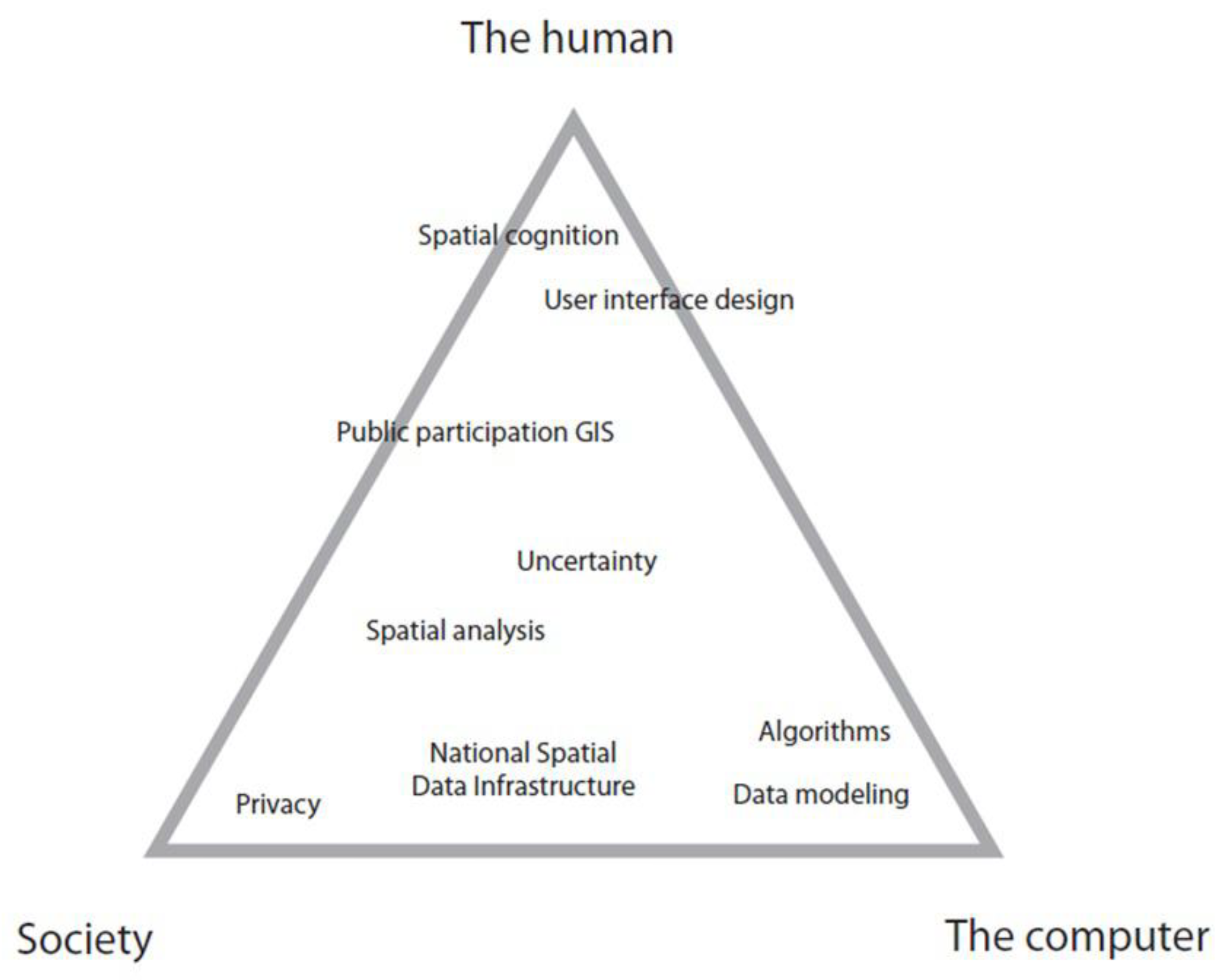
Figure 2.
Three representations of a temporal dimension in space: (a) a discretized space-time cube data architecture [35]; (b) a vectorized space-time cube depicting the Napoleonic Death March [36]; and (c) the evolution of a polygonal object in a vectorized layer against a temporal axis [37]. In (a) and (c), the temporal layering is discretized (how a GIS is typically envisioned architecturally), whereas in (b), there is no temporal layering at all, forming a continuous temporal dimension.
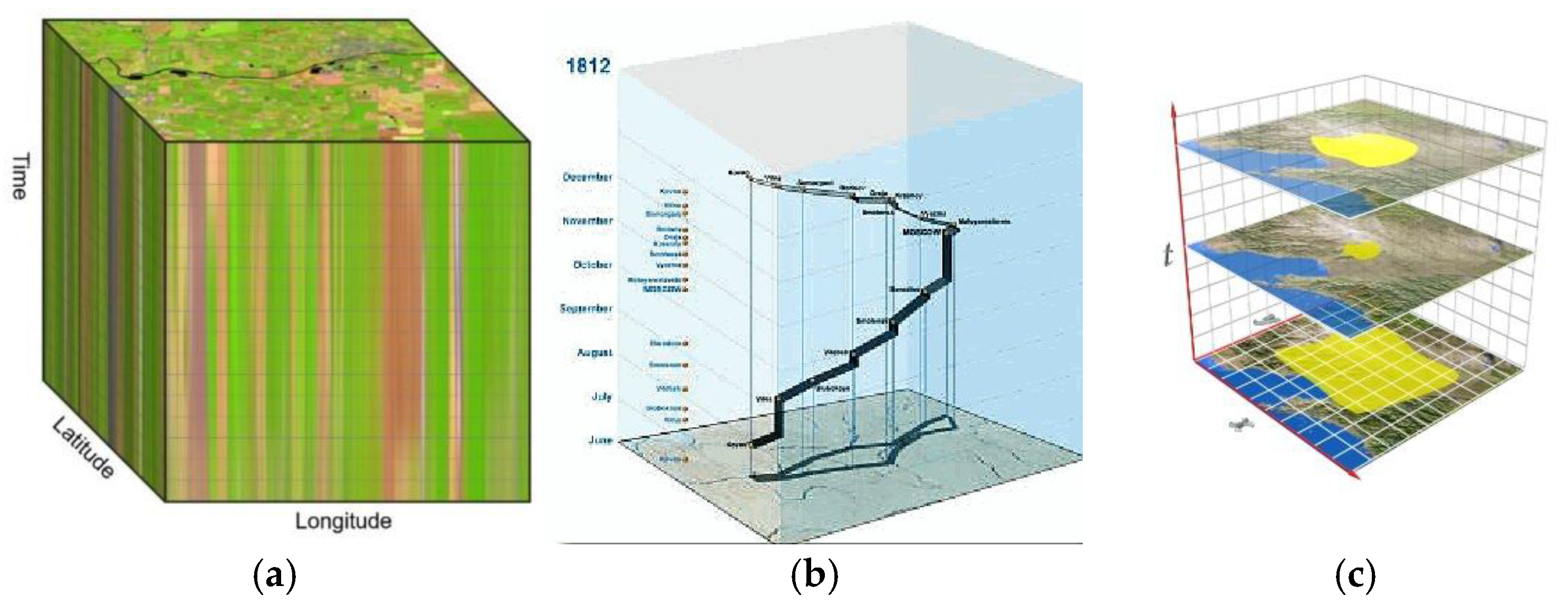
Figure 3.
Line segment in two-dimensional space treated topologically as if it came from a one-dimensional space.
Figure 3.
Line segment in two-dimensional space treated topologically as if it came from a one-dimensional space.
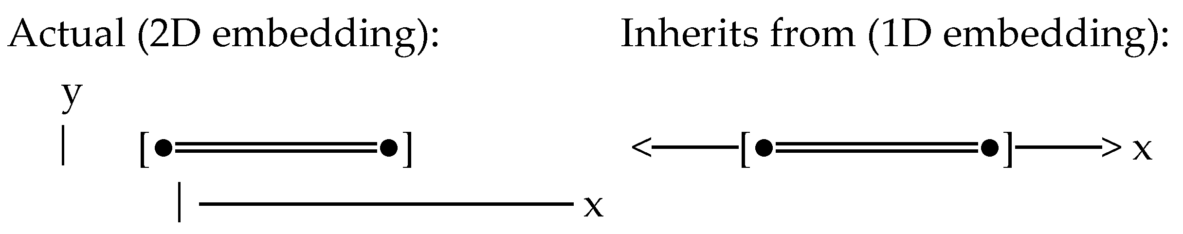
Figure 4.
Disconnected boundary points and exterior sectors in line segments.
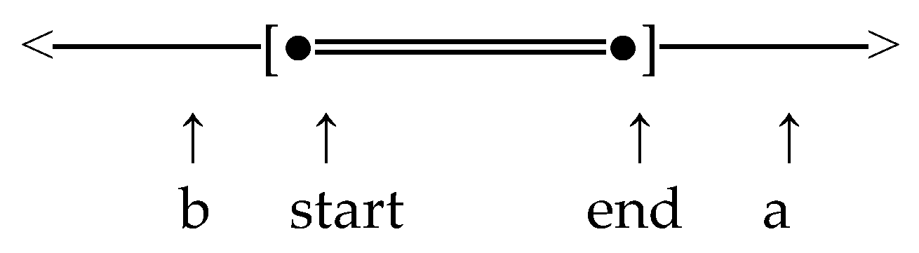
Figure 5.
Vocabulary mapping for identifiable components when an interval exists in a one-dimensional embedding space.
Figure 5.
Vocabulary mapping for identifiable components when an interval exists in a one-dimensional embedding space.
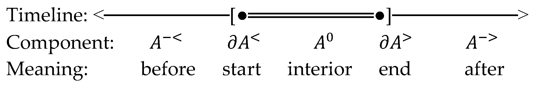
Figure 6.
Three homeomorphic deformations that can be applied to temporal intervals: (a) anisotropic scaling; (b) translation; and (c) isotropic scaling [55]. For intervals, anisotropic scaling is a monodirectional stretching or contraction of the object, translation is simply movement, and isotropic scaling is proportional growth/decline in both directions simultaneously.
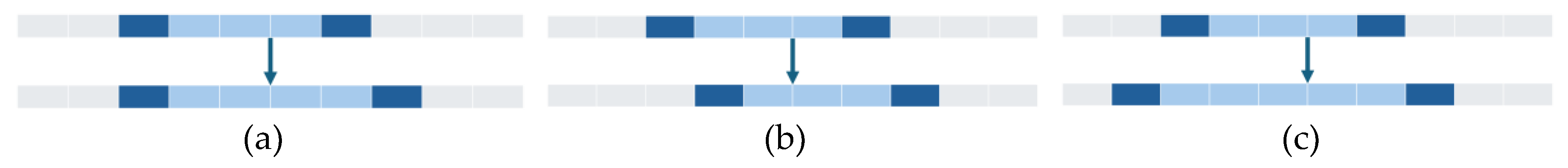
Figure 7.
Three distinct conceptual neighborhood graphs of the Allen interval relations, aligning with deformations of anisotropic scaling, translation, and isotropic scaling [19].
Figure 7.
Three distinct conceptual neighborhood graphs of the Allen interval relations, aligning with deformations of anisotropic scaling, translation, and isotropic scaling [19].
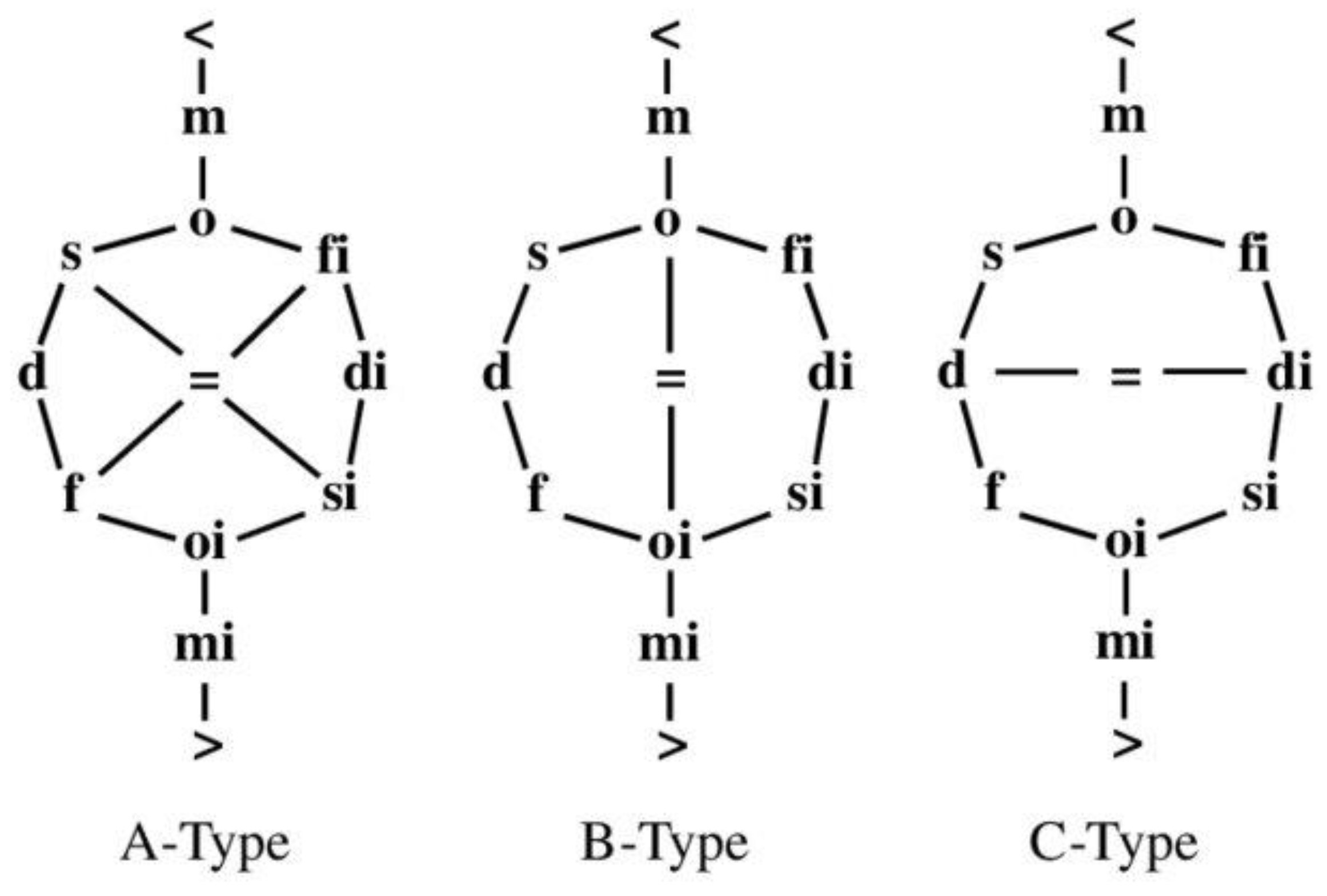
Figure 8.
Simulation protocol (adapted from [24,48]) for generating a test set of configurations with topological relations between two interval objects in
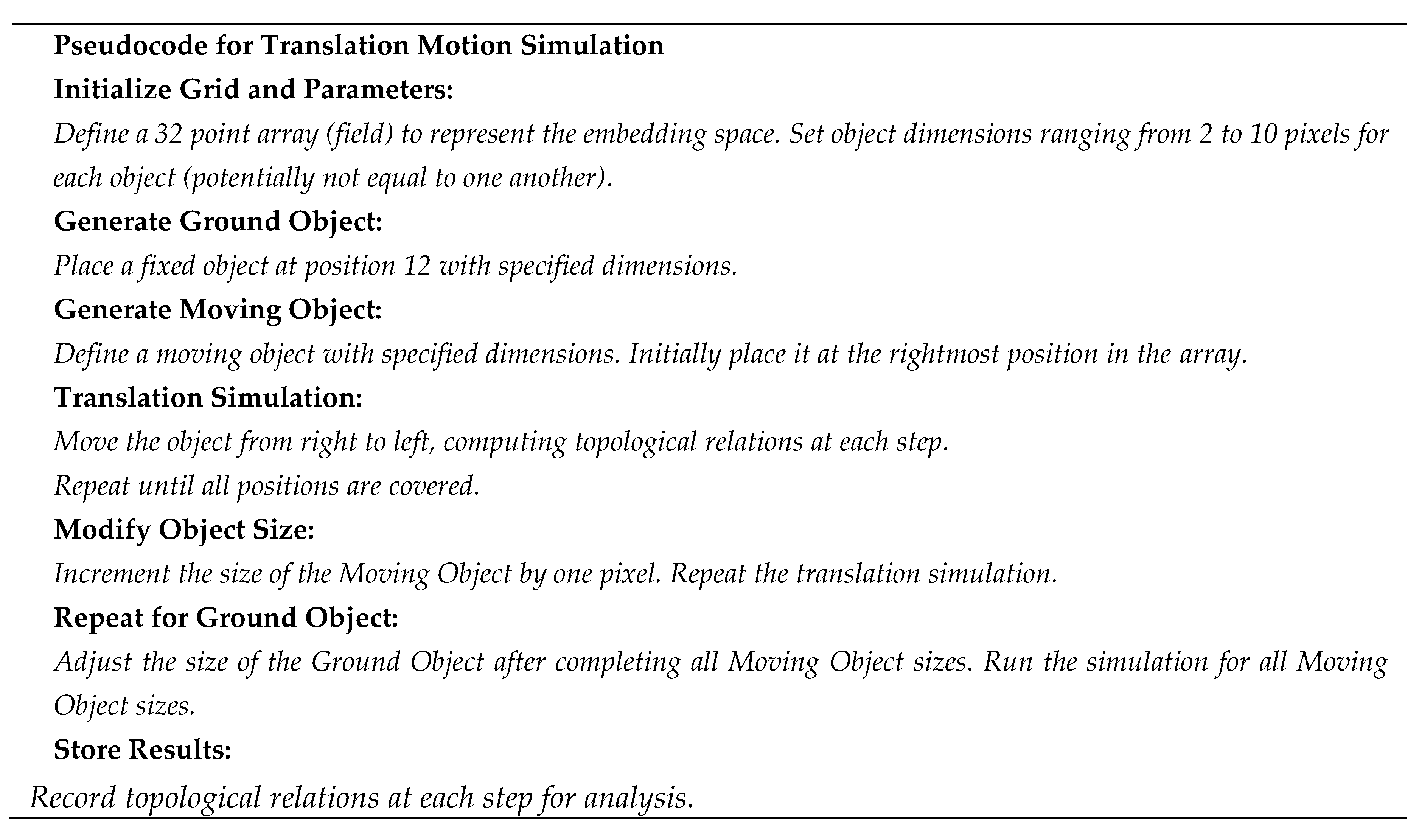
Figure 9.
Translation conceptual neighborhood graph derived from the simulation data. This graph is planar and is the only one to be disconnected because of the fixed sizes of the intervals in question in concert with the deformation not being able to change those fixed sizes. Each cluster in the graph represents various configurations of the presence of interior for both objects A and B.
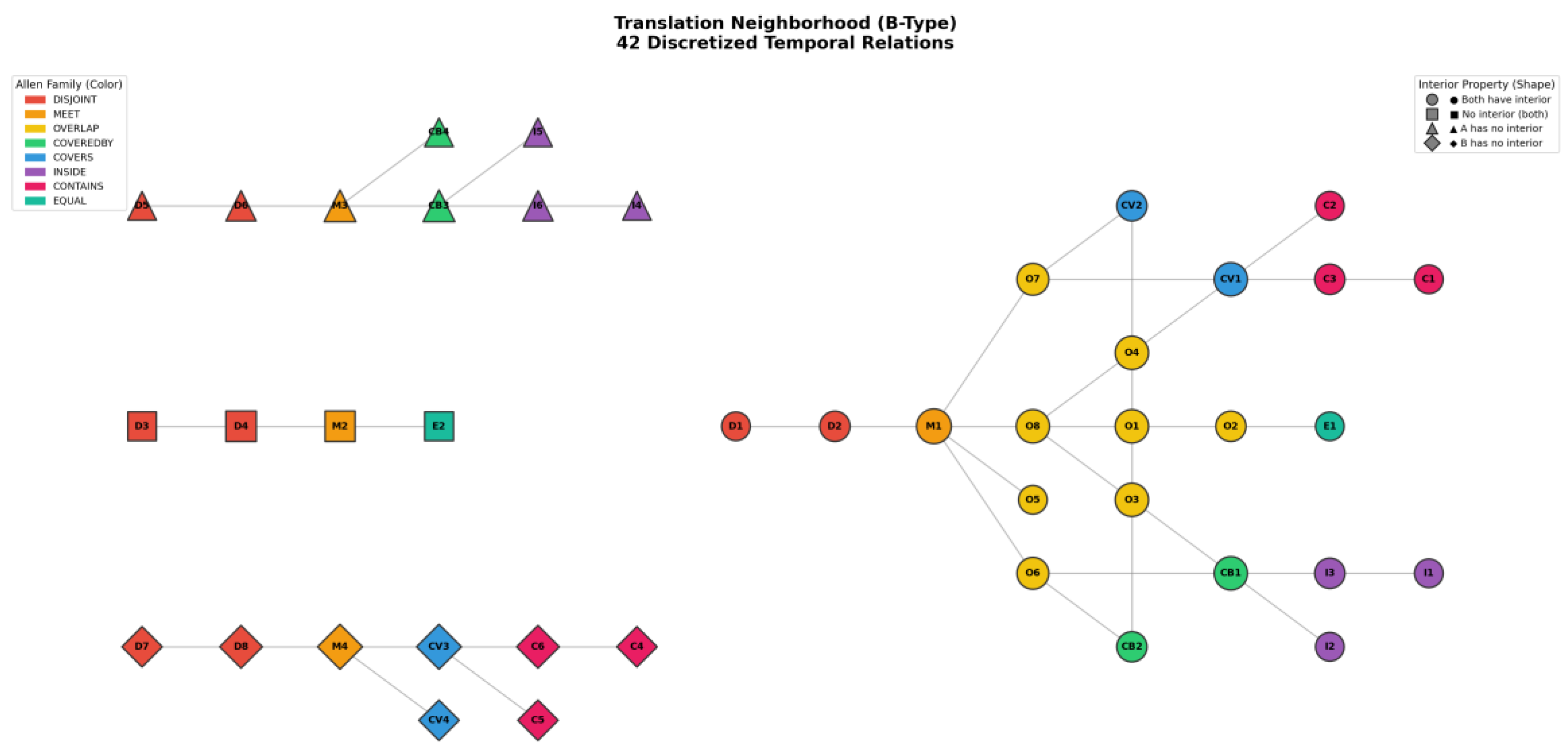
Figure 10.
Isotropic scaling conceptual neighborhood graph derived from the simulation data. Isotropic scaling demonstrates a different behavior of the connections (neighbors of different colors being possible or not), but maintains the symmetric property.
Figure 10.
Isotropic scaling conceptual neighborhood graph derived from the simulation data. Isotropic scaling demonstrates a different behavior of the connections (neighbors of different colors being possible or not), but maintains the symmetric property.
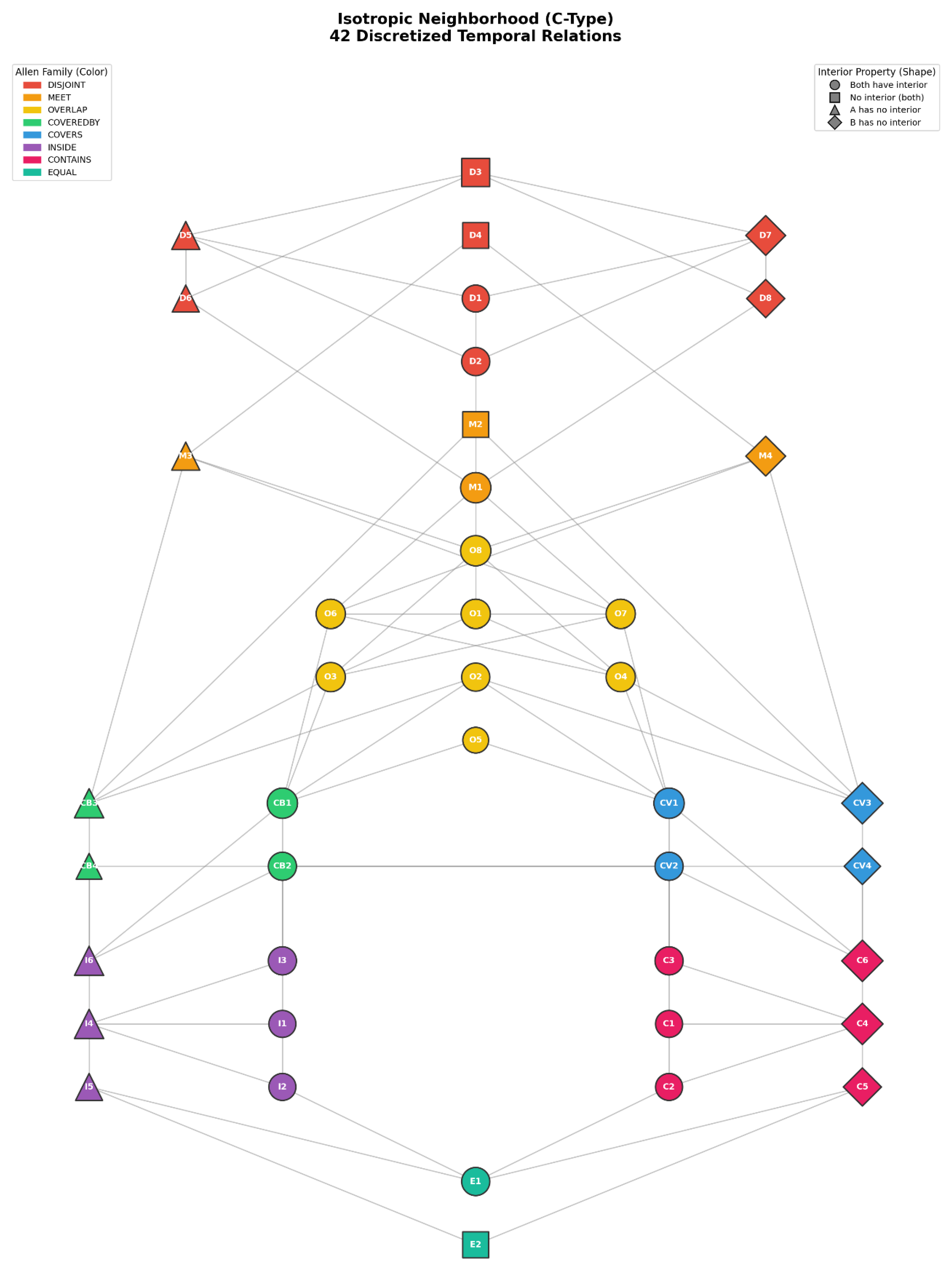
Figure 11.
Anisotropic scaling conceptual neighborhood graph derived from the simulation data. Similar to its isotropic counterpart, it is non-planar, symmetric, and follows the same consistent behavior of color-to-color progression.
Figure 11.
Anisotropic scaling conceptual neighborhood graph derived from the simulation data. Similar to its isotropic counterpart, it is non-planar, symmetric, and follows the same consistent behavior of color-to-color progression.
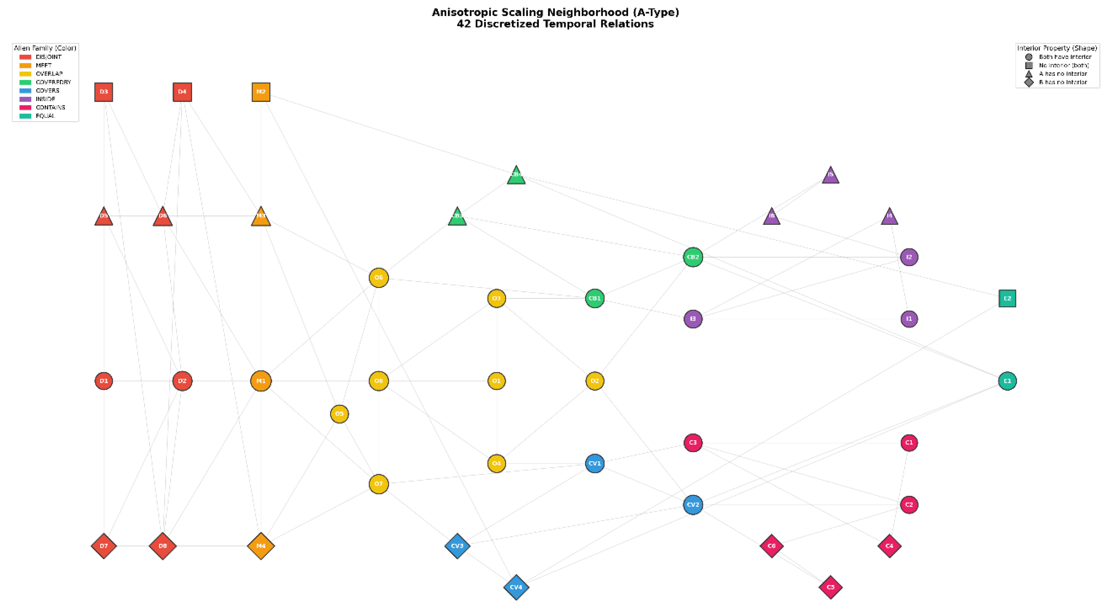
Figure 12.
Translation conceptual neighborhood graph of the discretized temporal relations. This neighborhood graph is generated by appending copies of the unordered translation conceptual neighborhood graph from Figure 9, glued together at the temporally symmetric relations.
Figure 12.
Translation conceptual neighborhood graph of the discretized temporal relations. This neighborhood graph is generated by appending copies of the unordered translation conceptual neighborhood graph from Figure 9, glued together at the temporally symmetric relations.
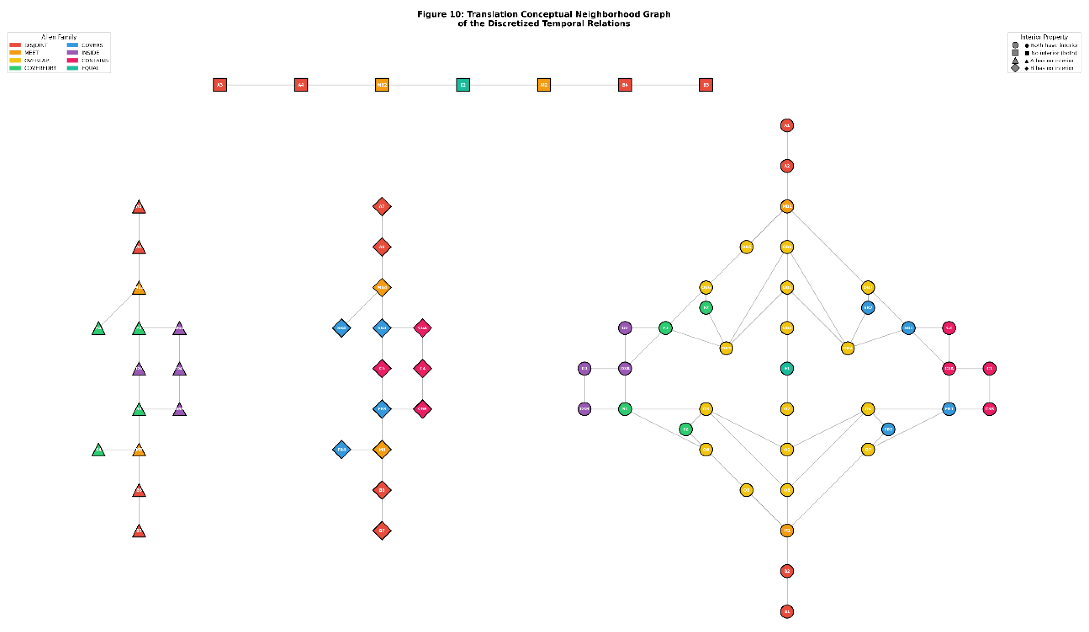
Figure 13.
Isotropic scaling conceptual neighborhood graph of the discretized temporal relations. This neighborhood graph is generated by appending copies of the unordered isotropic scaling conceptual neighborhood graph from Figure 10, glued together at the temporally symmetric relations.
Figure 13.
Isotropic scaling conceptual neighborhood graph of the discretized temporal relations. This neighborhood graph is generated by appending copies of the unordered isotropic scaling conceptual neighborhood graph from Figure 10, glued together at the temporally symmetric relations.
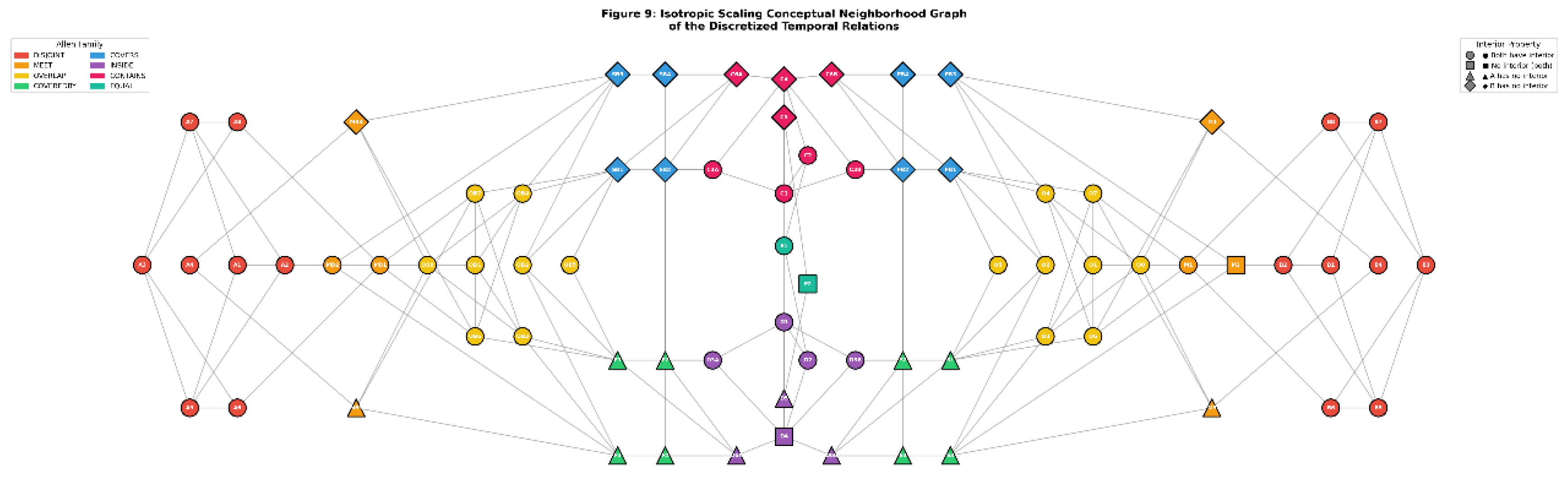
Figure 14.
Anisotropic scaling conceptual neighborhood graph of the discretized temporal relations. This neighborhood graph is generated by appending copies of the unordered anisotropic scaling conceptual neighborhood graph from Figure 11, glued together at the temporally symmetric relations.
Figure 14.
Anisotropic scaling conceptual neighborhood graph of the discretized temporal relations. This neighborhood graph is generated by appending copies of the unordered anisotropic scaling conceptual neighborhood graph from Figure 11, glued together at the temporally symmetric relations.
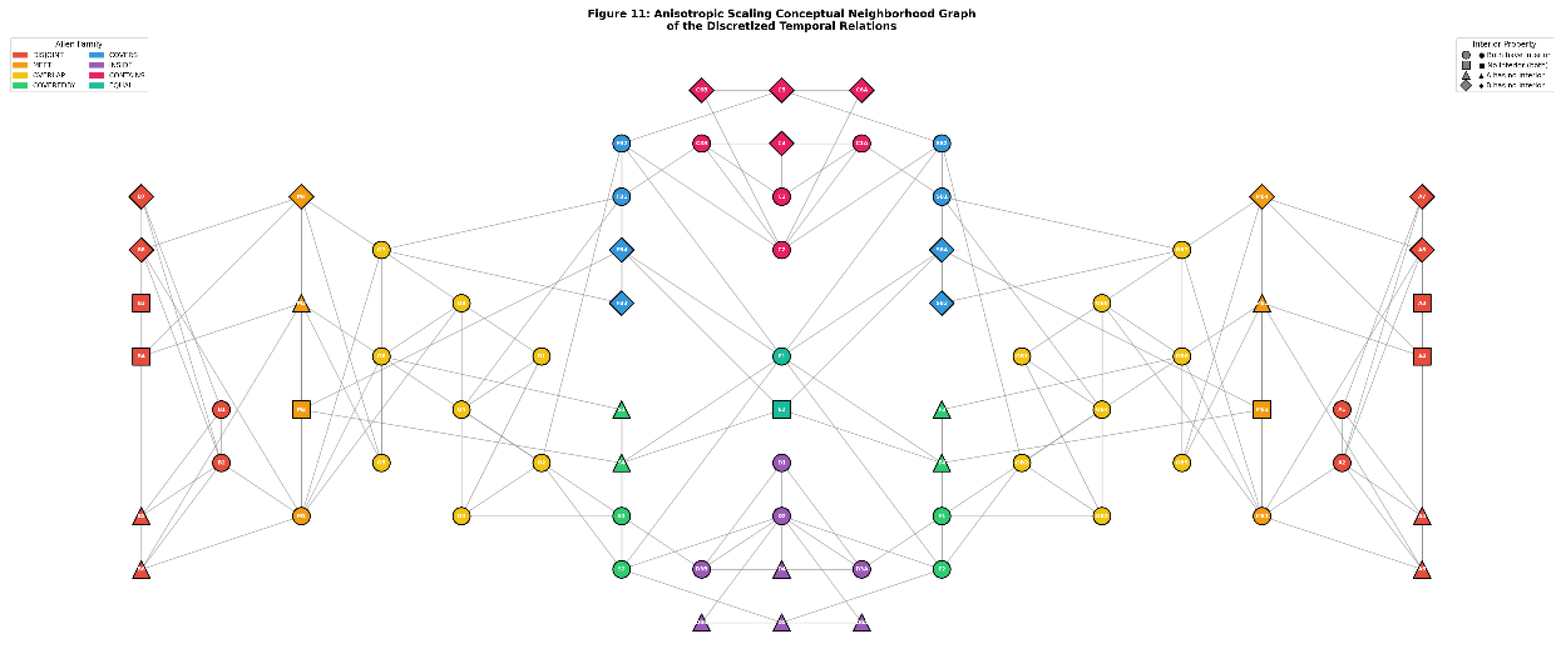
Figure 15.
The aggregated conceptual neighborhood graphs shown in (a) Table 11, (b) Table 9, and (c) Table 10, corresponding to the A-, B-, and C-neighborhoods [19,56]. The only difference between these graphs is the connection between coveredBy and covers in the C-neighborhood, the direct result of discretization.
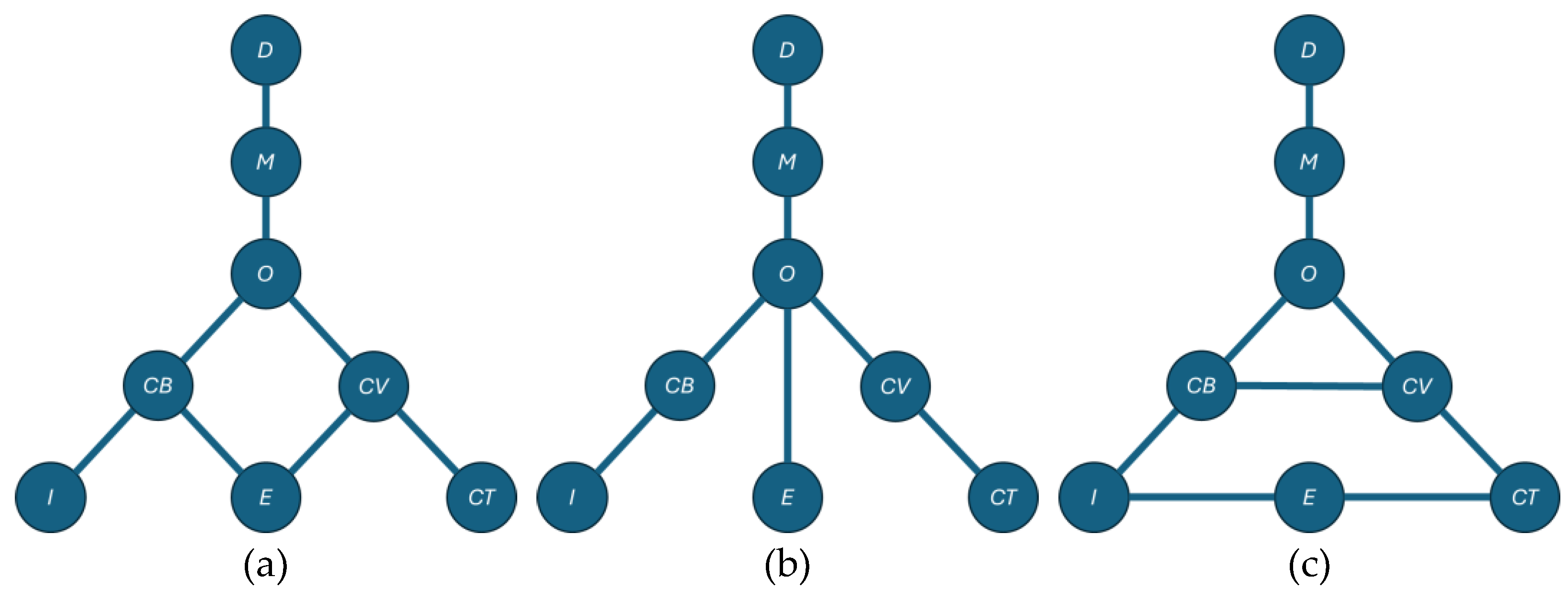
Figure 16.
A mapping of the Allen interval relations against properties of the relationships of their various endpoints. Various slices of this set of relations (conveniently organized by the basal structure of the conceptual neighborhood graphs of relations) share the same properties, with each relation itself being a unique intersection of a set of properties. By removing any one of the composite parts of the intersection logic, a set of relations rather than a singleton may occur [19].
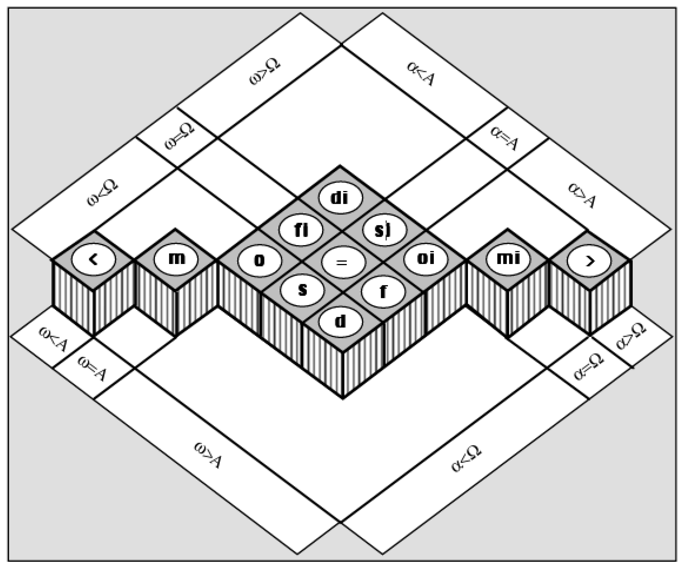
Figure 17.
Layered conceptual neighborhood graph of point-to-object direction symbols [53], an example of what conceptual neighborhood graphs should look like in a big-data age, emblematic of variety and cartographic generalization [61,62,63,64].
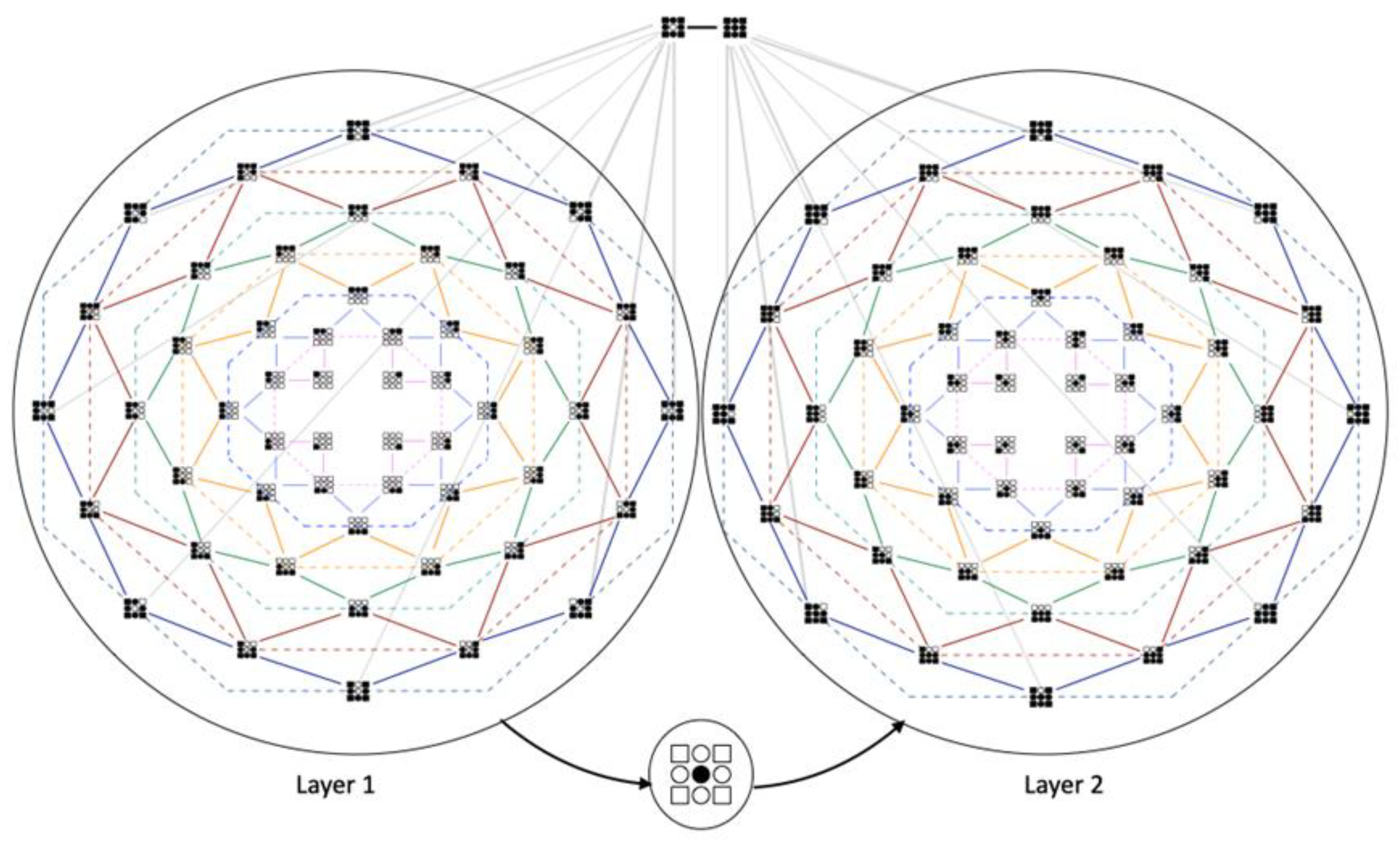
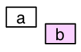 |
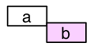 |
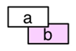 |
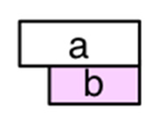 |
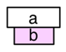 |
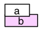 |
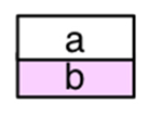 |
| before (<) | meets (m) | overlaps (o) | finished by (fi) | contains (di) | starts (s) | equal (=) |
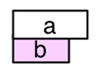 |
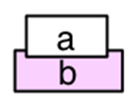 |
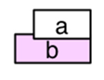 |
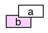 |
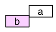 |
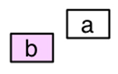 |
|
| started by (si) | during (d) | finishes (f) | overlapped by (oi) | met by (mi) | after (>) | |
Table 3.
Converse table of the Allen interval algebra [9]. Note that equal, contains, and during are temporally symmetric.
Table 3.
Converse table of the Allen interval algebra [9]. Note that equal, contains, and during are temporally symmetric.
| Non-Ordered Relation | Before Relation | After Relation (Mirror) |
|---|---|---|
| disjoint | before | after |
| meet | meets | met by |
| overlap | overlaps | overlapped by |
| coveredBy | starts | finishes |
| inside | during | during |
| covers | finished by | started by |
| contains | contains | contains |
| equal | equal | equal |
Table 4.
Discretized line-line relations in , organized by relational properties with respect to interior presence [14]. The blue group (rows 1-4) requires two objects both with interiors; the green group (row 5) requires two objects both without interiors; the red group (rows 6-9 left) requires an object A without an interior and an object B with an interior; the yellow group (rows 6-9 right) requires an object A with an interior and an object B without an interior. Relations that have a touch configuration to further refine them are denoted with an asterik. Each relation is given a shorthand name for visual purposes in Section 6 and Section 7.
|
disjoint* D1 (D2) 
|
meet M1 
|
equal E1 
|
contains* C1 (C3) 
|
containsTotal C2 
|
|||||
|
inside* I1 (I3) 
|
insideTotal I2 
|
overlap O1 
|
covers CV1 
|
coversTotal CV2 
|
|||||
|
coveredBy CB1 
|
coveredByTotal CB2 
|
overlapTotal O2 
|
overlapMeet O8 
|
overlapSmallA O6 
|
|||||
|
overlapSmallB O7 
|
overlapSmall O5 
|
overlapCovers O4 
|
overlapCoveredBy O3 
|
||||||
|
disjointNoInterior* D3 (D4) 
|
equalNoInterior E2 
|
meetNoInterior M2 
|
|||||||
|
disjointNoAInterior* D5 (D6) 
|
meetNoAInterior M3 
|
disjointNoBInterior* D7 (D8) 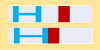
|
meetNoBInterior M4 
|
||||||
|
minimalCoveredBy CB3 
|
minimalInsideTotal I5 
|
minimalCovers CV3 
|
minimalContainsTotal C5 
|
||||||
|
minimalCoveredByTotal CB4 
|
minimalCoversTotal CV4 
|
||||||||
|
minimalInside* I4 (I6) 
|
minimalContains* C4 (C6) 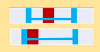
|
||||||||
Table 5.
Discretized temporal interval relations in , organized by Table 3 [14]. The blue group requires two objects both with interiors; the green group requires two objects both without interiors; the red group requires an object A without an interior and an object B with an interior; the yellow group requires an object A with an interior and an object B without an interior. Relations follow the numbering convention from Table 3. Touch relations originating from disjoint are not distinguishable via the 9+-intersection. Each relation is given a shorthand name for visual purposes in Section 6 and Section 7 that relates to its relation from Table 3 (e.g., D1 from Table 4 becomes B1 and A1, accounting for the temporal ordering).
| Parent Relation | Symbolic and Graphical Representation | Parent Converse | Symbolic and Graphical Representation | ||
|---|---|---|---|---|---|
|
before (from disjoint) |
B1 
|
B2 
|
after |
A1 
|
A2 
|
|
B3 
|
B4 
|
A3 
|
A4 
|
||
|
B5 
|
B6 
|
A5 
|
A6 
|
||
|
B7 
|
B8 
|
A7 
|
A8 
|
||
|
meet (from meet) |
M1 
|
M2 
|
met by |
MB1 
|
MB2 
|
|
M3 
|
M4 
|
MB3 
|
MB4 
|
||
|
overlaps (from overlap) |
O1 
|
O2 
|
overlapped by |
OB1 
|
OB2 
|
|
O3 
|
O4 
|
OB3 
|
OB4 
|
||
|
O5 
|
O6 
|
OB5 
|
OB6 
|
||
|
O7 
|
O8 
|
OB7 
|
OB8 
|
||
|
starts (from coveredBy) |
S1 
|
S2 
|
finishes |
F1 
|
F2 
|
|
S3 
|
S4 
|
F3 
|
F4 
|
||
|
during (from inside) |
D1 
|
D2 
|
during | -same- | -same- |
|
D4 
|
D5 
|
-same | -same | ||
|
D3A 
|
D6A 
|
D3B 
|
D6B 
|
||
|
finished by (from covers) |
FB1 
|
FB2 
|
started by |
SB1 
|
SB2 
|
|
FB3 
|
FB4 
|
SB3 
|
SB4 
|
||
|
contains (from contains) |
C1 
|
C2 
|
contains | -same- | -same- |
|
C4 
|
C5 
|
-same- | -same- | ||
|
C3A 
|
C6A 
|
C3B 
|
C6B 
|
||
|
equal (from equal) |
E1 
|
E2 
|
equal | -same- | -same- |
Table 6.
Translation conceptual neighborhood graph in Figure 9 as an edge list. Each relation that is the converse of another relation in the set relates to the converse relations to the relations that the original relation connects to.
Table 6.
Translation conceptual neighborhood graph in Figure 9 as an edge list. Each relation that is the converse of another relation in the set relates to the converse relations to the relations that the original relation connects to.
| Relation | Connected Relations | Converse Relation | Connected Relations |
|---|---|---|---|
| D1 | D2 | ||
| D2 | D1, M1 | ||
| D3 | D4 | ||
| D4 | D3, M2 | ||
| D5 | D6 | D7 | D8 |
| D6 | D5, M3 | D8 | D7, M4 |
| M1 | D2, O5, O6, O7, O8 | ||
| M2 | D4, E2 | ||
| M3 | D6, CB3, CB4 | M4 | D8, CV3, CV4 |
| O1 | O2, O3, O4, O8 | ||
| O2 | O1, E1 | ||
| O3 | O1, O8, CB1, CB2 | O4 | O1, O8, CV1, CV2 |
| O5 | M1 | ||
| O6 | M1, CB1, CB2 | O7 | M1, CV1, CV2 |
| O8 | M1, O1, O3, O4 | ||
| CB1 | O3, O6, I2, I3 | CV1 | O4, O7, C2, C3 |
| CB2 | O3, O6 | CV2 | O4, O7 |
| CB3 | M3, I5, I6 | CV3 | M4, C5, C6 |
| CB4 | M3 | CV4 | M4 |
| I1 | I3 | C1 | C3 |
| I2 | CB1 | C2 | CV1 |
| I3 | CB1, I1 | C3 | CV1, C1 |
| I4 | I6 | C4 | C6 |
| I5 | CB3 | C5 | CV3 |
| I6 | CB3, I4 | C6 | CV3, C4 |
| E1 | O2 | ||
| E2 | M2 |
Table 7.
Isotropic conceptual neighborhood graph in Figure 10 as an edge list. Each relation that is the converse of another relation in the set relates to the converse relations to the relations that the original relation connects to.
Table 7.
Isotropic conceptual neighborhood graph in Figure 10 as an edge list. Each relation that is the converse of another relation in the set relates to the converse relations to the relations that the original relation connects to.
| Relation | Connected Relations | Converse Relation | Connected Relations |
|---|---|---|---|
| D1 | D2, D5, D7 | ||
| D2 | D1, D5, D7, M1 | ||
| D3 | D5, D6, D7, D8 | ||
| D4 | M3, M4 | ||
| D5 | D1, D2, D3, D6 | D7 | D1, D2, D3, D8 |
| D6 | D3, D5, M1 | D8 | D3, D7, M1 |
| M1 | D2, D6, D8, O6, O7, O8 | ||
| M2 | CB3, CV3 | ||
| M3 | D4, O7, O8, CB3 | M4 | D4, O6, O8, CV3 |
| O1 | O3, O4, O6, O7, O8 | ||
| O2 | CB1, CB3, CV1, CV3 | ||
| O3 | O1, O7, O8, CB1, CB3 | O4 | O1, O6, O8, CV1, CV3 |
| O5 | CB1, CV1 | ||
| O6 | M1, M4, O1, O4, CB1 | O7 | M1, M3, O1, O3, CV1 |
| O8 | M1, M3, M4, O1, O3, O4 | ||
| CB1 | O2, O3, O5, O6, I3, I6 | CV1 | O2, O4, O5, O7, C3, C6 |
| CB2 | CV2, CV4, I3, I6 | CV2 | CB2, CB4, C3, C6 |
| CB3 | M2, M3, O2, O3, I6 | CV3 | M2, M4, O2, O4, C6 |
| CB4 | CV2, I6 | CV4 | CB2, C6 |
| I1 | I2, I3, I4 | C1 | C2, C3, C4 |
| I2 | I1, I4, E1 | C2 | C1, C4, E1 |
| I3 | CB1, CB2, I1, I4 | C3 | CV1, CV2, C1, C4 |
| I4 | I1, I2, I3, I5, I6 | C4 | C1, C2, C3, C5, C6 |
| I5 | I4, E1, E2 | C5 | C4, E1, E2 |
| I6 | CB1, CB2, CB3, CB4, I4 | C6 | CV1, CV2, CV3, CV4, C6 |
| E1 | I2, I5, C2, C5 | ||
| E2 | I5, C5 |
Table 8.
Anisotropic conceptual neighborhood graph in Figure 11 as an edge list. Each relation that is the converse of another relation in the set relates to the converse relations to the relations that the original relation connects to.
Table 8.
Anisotropic conceptual neighborhood graph in Figure 11 as an edge list. Each relation that is the converse of another relation in the set relates to the converse relations to the relations that the original relation connects to.
| Relation | Connected Relations | Converse Relation | Connected Relations |
| D1 | D2, D5, D7 | ||
| D2 | D1, D5, D6, D7, D8, M1 | ||
| D3 | D5, D6, D7, D8 | ||
| D4 | D6, D8, M3, M4 | ||
| D5 | D1, D2, D3, D6 | D7 | D1, D2, D3, D8 |
| D6 | D2, D3, D4, D5, M1, M3 | D8 | D2, D3, D4, D7, M1, M4 |
| M1 | D2, D6, D8, M3, M4, O6, O7, O8 | ||
| M2 | M2, M3, CB4, CV4 | ||
| M3 | D4, D6, M1, M2, O5, O6 | M4 | D4, D8, M1, M2, O5, O7 |
| O1 | O3, O4, O8 | ||
| O2 | O3, O4, CB2, CV2 | ||
| O3 | O1, O2, O8, CB1 | O4 | O1, O2, O8, CV1 |
| O5 | O6, O7, M3, M4 | ||
| O6 | M1, M3, O5, O8, CB1, CB3 | O7 | M1, M4, O5, O8, CV1, CV3 |
| O8 | M1, O1, O3, O4, O6, O7 | ||
| CB1 | O3, O6, CB2, CB3, I3 | CV1 | O4, O7, CV2, CV3, C3 |
| CB2 | O2, CB1, CB3, I2, I5, E1 | CV2 | O2, CV1, CV3, C2, C5, E1 |
| CB3 | O6, CB1, CB2, CB4 | CV3 | O7, CV1, CV2, CV4 |
| CB4 | M2, CB3, E1, E2 | CV4 | M2, CV3, E1, E2 |
| I1 | I3, I4 | C1 | C3, C4 |
| I2 | CB2, I3, I6 | C2 | CV2, C3, C6 |
| I3 | CB1, I1, I2, I4 | C3 | CV1, C1, C2, C4 |
| I4 | I1, I3 | C4 | C1, C3 |
| I5 | CB2, I6 | C5 | CV2, C6 |
| I6 | I2, I5 | C6 | C2, C5 |
| E1 | CB2, CB4, CV2, CV4 | ||
| E2 | CB4, CV4 |
Table 9.
Translation conceptual neighborhood graph from Table 6 mapped to its corresponding relational groups from the continuous line-line relations by removing the numerical designations.
Table 9.
Translation conceptual neighborhood graph from Table 6 mapped to its corresponding relational groups from the continuous line-line relations by removing the numerical designations.
| Relation | Connected Relations | Converse Relation | Connected Relations |
|---|---|---|---|
| D | D | ||
| D | D, M | ||
| D | D | ||
| D | D, M | ||
| D | D | D | D |
| D | D, M | D | D, M |
| M | D, O, O, O, O | ||
| M | D, E | ||
| M | D, CB, CB | M | D, CV, CV |
| O | O, O, O, O | ||
| O | O, E | ||
| O | O, O, CB, CB | O | O, O, CV, CV |
| O | M | ||
| O | M, CB, CB | O | M, CV, CV |
| O | M, O, O, O | ||
| CB | O, O, I, I | CV | O, O, C, C |
| CB | O, O | CV | O, O |
| CB | M, I, I | CV | M, C, C |
| CB | M | CV | M |
| I | I | C | C |
| I | CB | C | CV |
| I | CB, I | C | CV, C |
| I | I | C | C |
| I | CB | C | CV |
| I | CB, I | C | CV, C |
| E | O | ||
| E | M |
Table 10.
Isotropic conceptual neighborhood graph from Table 7 mapped to its corresponding relational groups from the continuous line-line relations by removing the numerical designations.
Table 10.
Isotropic conceptual neighborhood graph from Table 7 mapped to its corresponding relational groups from the continuous line-line relations by removing the numerical designations.
| Relation | Connected Relations | Converse Relation | Connected Relations |
|---|---|---|---|
| D | D, D, D | ||
| D | D, D, D, M | ||
| D | D, D, D, D | ||
| D | M, M | ||
| D | D, D, D, D | D | D, D, D, D |
| D | D, D, M | D | D, D, M |
| M | D, D, D, O, O, O | ||
| M | CB, CV | ||
| M | D, O, O, CB | M | D, O, O, CV |
| O | O, O, O, O, O | ||
| O | CB, CB, CV, CV | ||
| O | O, O, O, CB, CB | O | O, O, O, CV, CV |
| O | CB, CV | ||
| O | M, M, O, O, CB | O | M, M, O, O, CV |
| O | M, M, M, O, O, O | ||
| CB | O, O, O, O, I, I | CV | O, O, O, O, C, C |
| CB | CV, CV, I, I | CV | CB, CB, C, C |
| CB | M, M, O, O, I | CV | M, M, O, O, C |
| CB | CV, I | CV | CB, C |
| I | I, I, I | C | C, C, C |
| I | I, I, E | C | C, C, E |
| I | CB, CB, I, I | C | CV, CV, C, C |
| I | I, I, I, I, I | C | C, C, C, C, C |
| I | I, E, E | C | C, E, E |
| I | CB, CB, CB, CB, I | C | CV, CV, CV, CV, C |
| E | I, I, C, C | ||
| E | I, C |
Table 11.
Anisotropic conceptual neighborhood graph from Table 8 mapped to its corresponding relational groups from the continuous line-line relations by removing the numerical designations.
Table 11.
Anisotropic conceptual neighborhood graph from Table 8 mapped to its corresponding relational groups from the continuous line-line relations by removing the numerical designations.
| Relation | Connected Relations | Converse Relation | Connected Relations |
|---|---|---|---|
| D | D, D, D | ||
| D | D, D, D, D, D, M | ||
| D | D, D, D, D | ||
| D | D, D, M, M | ||
| D | D, D, D, D | D | D, D, D, D |
| D | D, D, D, D, M, M | D | D, D, D, D, M, M |
| M | D, D, D, M, M, O, O, O | ||
| M | M, M, CB, CV | ||
| M | D, D, M, M, O, O | M | D, D, M, M, O, O |
| O | O, O, O | ||
| O | O, O, CB, CV | ||
| O | O, O, O, CB | O | O, O, O, CV |
| O | O, O, M, M | ||
| O | M, M, O, O, CB, CB | O | M, M, O, O, CV, CV |
| O | M, O, O, O, O, O | ||
| CB | O, O, CB, CB, I | CV | O, O, CV, CV, C |
| CB | O, CB, CB, I, I, E | CV | O, CV, CV, C, C, E |
| CB | O, CB, CB, CB | CV | O, CV, CV, CV |
| CB | M, CB, E, E | CV | M, CV, E, E |
| I | I, I | C | C, C |
| I | CB, I, I | C | CV, C, C |
| I | CB, I, I, I | C | CV, C, C, C |
| I | I, I | C | C, C |
| I | CB, I | C | CV, C |
| I | I, I | C | C, C |
| E | CB, CB, CV, CV | ||
| E | CB, CV |
Disclaimer/Publisher’s Note: The statements, opinions and data contained in all publications are solely those of the individual author(s) and contributor(s) and not of MDPI and/or the editor(s). MDPI and/or the editor(s) disclaim responsibility for any injury to people or property resulting from any ideas, methods, instructions or products referred to in the content. |
© 2026 by the authors. Licensee MDPI, Basel, Switzerland. This article is an open access article distributed under the terms and conditions of the Creative Commons Attribution (CC BY) license.
Copyright: This open access article is published under a Creative Commons CC BY 4.0 license, which permit the free download, distribution, and reuse, provided that the author and preprint are cited in any reuse.


