Preprint
Article

This version is not peer-reviewed.

Machine Learning Approaches for Assessing Avocado Alternate Bearing Using Sentinel-2 and Climate Variables—A Case Study in Limpopo, South Africa

A peer-reviewed article of this preprint also exists.

Submitted:

30 October 2025

Posted:

31 October 2025

You are already at the latest version

Abstract

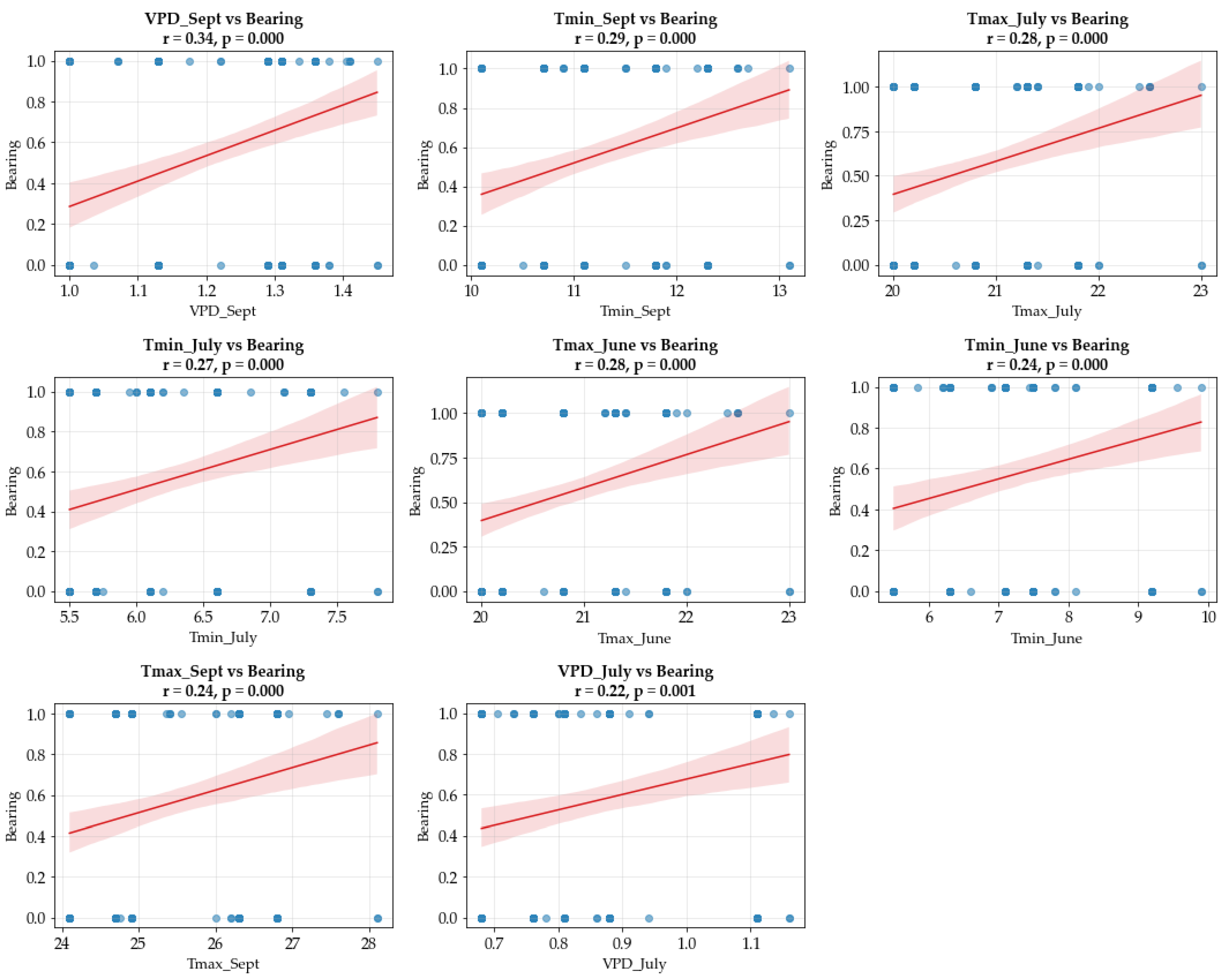
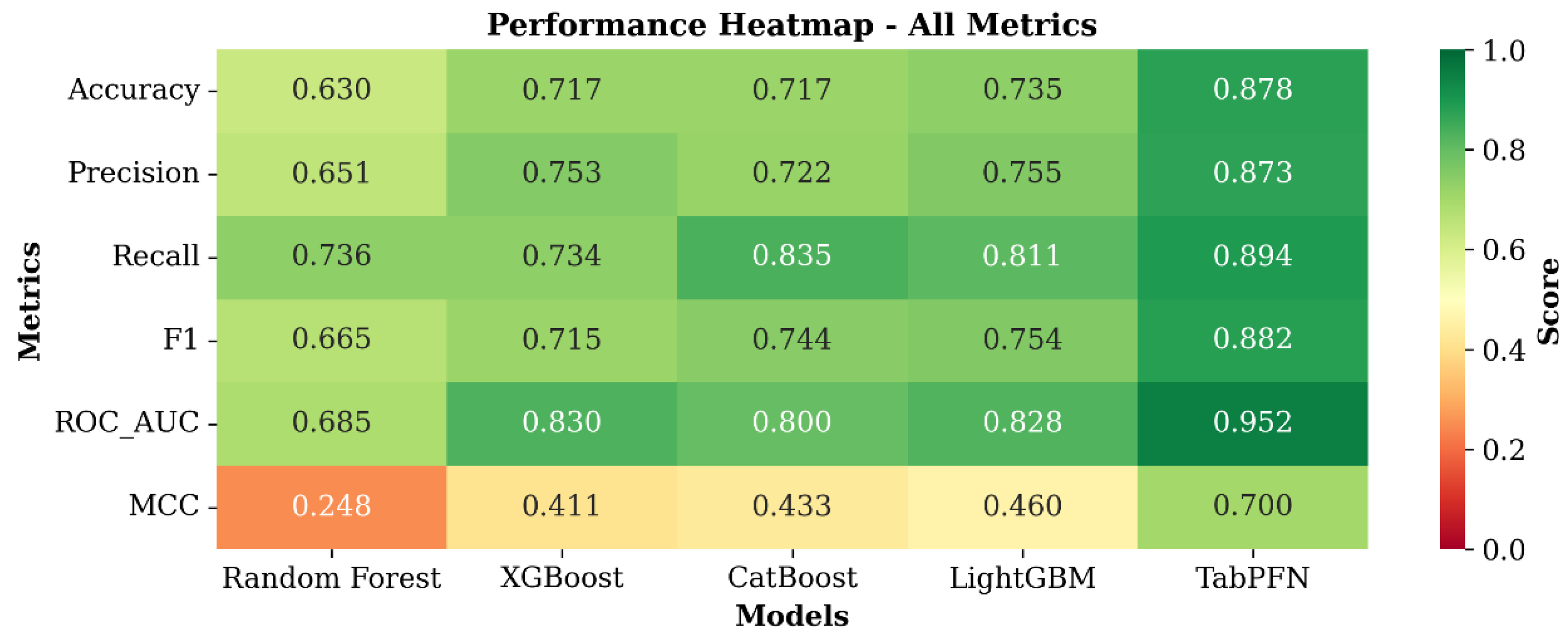
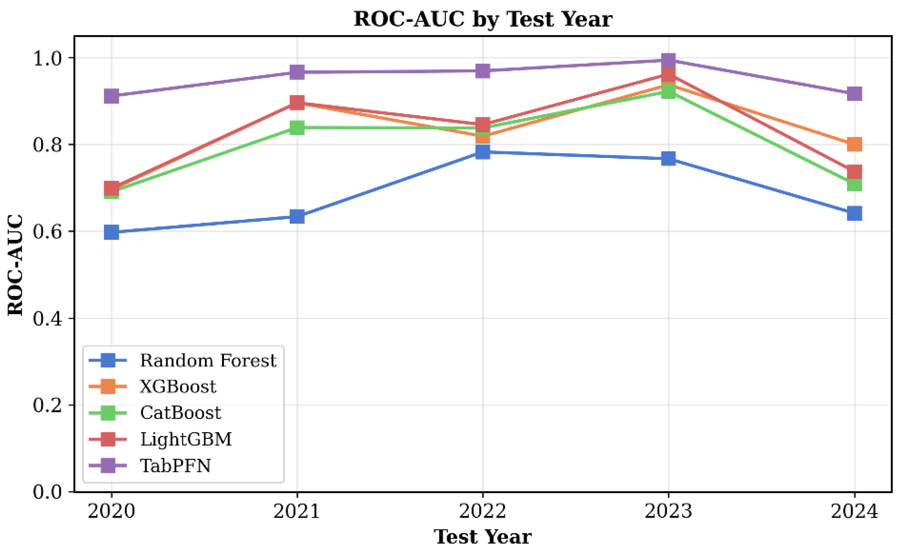
Alternate (irregular) bearing, characterized by large fluctuations in fruit yield between consecutive years, remains a major constraint to sustainable avocado (Persea americana) production. This study aimed to assess the potential of satellite remote sensing and climatic variables to characterize and predict alternate bearing patterns in commercial orchards in Tzaneen, Limpopo Province, South Africa. Historical yield data (2018–2024) from 46 ‘Hass’ avocado blocks were analyzed alongside Sentinel-2 derived vegetation indices (NDVI, GNDVI, NDRE, CIG, CIRE, EVI2, LSWI) and flowering indices (WYI, NDYI, MTYI). Climatic predictors including maximum temperature (Tmax), minimum temperature (Tmin), vapour pressure deficit (VPD), and precipitation were incorporated. Five machine learning algorithms—Random Forest, XGBoost, CATBoost, LightGBM, and TabPFN—were trained and tested using a Leave-One-Year-Out (LOYO) approach. Results showed that VPD, Tmin, and Tmax during the flowering period (July–September) were the most influential variables affecting subsequent yields. TabPFN achieved the highest predictive accuracy (Accuracy = 0.88; AUC = 0.95) and strongest temporal generalization. Spectral gradients between flowering and early fruit drop were lower during “on” years, reflecting stable canopy vigour. These findings demonstrate that integrating remote sensing and climatic indicators enables early discrimination of “on” and “off” years, supporting proactive orchard management and improved yield stability.

Keywords: 
;  ;  ;  ;  ;  ;  ;  

1. Introduction

Avocado (Persea americana Mill.) is one of the fastest growing fruit crops globally, gaining recognition for its nutritional value, popularity in variety of recipes and economic benefits. The global avocado production has expanded dramatically in the past two decades, reaching around 10.9 million metric tons in 2023 [1]. Leading producers include Mexico, Colombia, Peru, Dominican Republic, and Kenya, while emerging regions in Africa and Asia are increasingly contributing to global supply [2]. South Africa ranks among the top nine (2.1%) major avocado exporting countries, due to its subtropical climate, fertile soils, and comprehensive agronomic practices [3]. Avocados play a critical role in the country’s horticultural exports and rural economic development [4,5].
However, a persistent challenge undermining sustainable avocado production in South Africa and globally is alternate bearing, also referred to as irregular or biennial bearing. Alternate bearing (AB) is hypothesised to be a physiological phenomenon in which fruit trees produce a heavy yield one year (“on” year), followed by a substantially reduced or failed yield in the subsequent year (“off” year) [6]. Notably, AB does not always follow a strict biennial pattern; in some cases, it can occur in longer cycles, such as every two or three years. Although common in perennial fruit trees, this pattern makes it hard to predict yields, manage resources, and maintain stable markets, which can affect the economic profitability of commercial orchards [7,8].
The causes of AB are multifactorial and include intrinsic hormonal signals, nutrient allocation, environmental stressors and previous fruit load among others [9,10,11]. During an “on” year, excessive carbohydrate and nutrient investment into fruit development often depletes reserves needed for flower initiation in the following season, perpetuating the AB cycle. Additionally, environmental constraints such as drought, temperature extremes, and diseases and pest pressure may exacerbate this pattern [11,12]. This leads to major fluctuations in production and instability in the national avocado supply chain. From a sustainability perspective, AB affects not only yield consistency but also the efficient use of water, fertilizer, and labor, all of which are increasingly important from the perspective of climate resilience and sustainable farming practices [13]. Addressing AB is thus central to improving productivity, better management, and ensuring long-term orchard sustainability.
Conventional approaches to diagnosing AB rely on manual inspection, yield records, and visual phenology assessments [6,13]. While useful, these methods are labor-intensive, subjective, and often lack scalability across large commercial orchards. As the agricultural sector increasingly transitions toward digital and data-driven solutions, there is growing interest in leveraging remote sensing and machine learning (ML) technologies to enhance crop monitoring and decision-making [14,15].
Remote sensing technologies, particularly satellite-based platforms, have emerged as transformative tools in precision agriculture. Satellite remote sensing enables frequent, large-scale, and non-destructive observation of agricultural fields, offering valuable insights into vegetation health, crop yield potential, and phenological stages [16,17]. Among these platforms, the Sentinel-2 mission developed by the European Space Agency (ESA), has gained widespread use due to its high spatial resolution (10–20 meters), frequent revisit time (every 3 to 5 days) enabled by the twin satellites Sentinel-2A and 2B and their overlapping, and its 13-band multispectral imaging capabilities [17,18]. Sentinel-2 data support a variety of vegetation indices (VIs) that are correlated with biophysical crop parameters such as chlorophyll content, leaf area index (LAI), and canopy structure. The Normalized Difference Vegetation Index (NDVI) is the most widely used, to estimate vegetative vigour and biomass [19]. While NDVI is robust and broadly applicable, it may saturate under dense canopies and lacks sensitivity to subtle physiological changes [16,20]. To overcome such limitations, other indices like the Green Normalized Difference Vegetation Index (GNDVI), Normalized Difference Red Edge Index (NDRE), Chlorophyll Index Green (CIG), Chlorophyll Index Red Edge (CIRE), Enhance Vegetation Index 2 (EVI2) among others have been developed, particularly for perennial and woody crops [21,22,23,24].
The VIs are effective tools for monitoring canopy vigour and general plant health; however, they often fall short in capturing reproductive phenology, such as flowering and fruit set, which are central to understanding AB in perennial crops like avocado (Persea americana) [11,25]. Given the central role of reproductive development in AB, integrating flowering sensitive spectral indices provides an opportunity to enhance remote sensing based detection of “on” year and “off” year crops in avocado orchards. Recent advancements in spectral analysis have led to the development of flowering sensitive indices that focus on the optical properties of flowers, including their color, reflectance, and structural differences relative to foliage. The Weighted Yellowness Index (WYI) is specifically designed to enhance the detection of flowering by assigning greater weight to spectral bands associated with floral signals, while minimizing the contribution of bands dominated by chlorophyll and vegetation greenness [26]. The Normalized Difference Yellowness Index (NDYI) utilizes reflectance in the green and blue wavelengths to distinguish inflorescence areas from the surrounding canopy, offering an effective means of separating reproductive structures from vegetative background [27]. The Mango tree Yellowness Index (MTYI) serves as another flowering sensitive index that captures the yellow spectral response observed in flowering tree canopies and has shown promise in representing reproductive phenology in tropical fruit trees [26]. The integration of flowering indices (FIs) with traditional VIs offers a more holistic view of both vegetative and reproductive processes in avocado orchards. This is particularly valuable for detecting alternations between “on” year and “off” year cycles, where the extent of flowering and subsequent fruit retention following early fruit drop serve as critical indicators of AB behavior [25,28].
A number of previous studies have reported the significant influence of climate variables in initiating and reinforcing AB patterns in avocado (Persea americana Mill.) production systems in different ways for different regions [29,30,31,32]. Temperature extremes constitute one of the primary climatic factors influencing this phenomenon, as exposure to temperatures exceeding 40°C can cause severe physiological damage and stress, particularly during late summer heat waves [33]. According to Gafni [34], temperatures higher than 42°C are unfavourable for avocado production. Additionally, if temperatures rise up to and above 30°C for a number of days, it would adversely affect flowering phenology and fruit quality through mechanisms involving water stress and cellular dehydration, while low temperatures can similarly disrupt reproductive processes and reduce fruit set [33,35]. According to Sedgley and Grant [36], temperatures less than 12°C can affect flowering and reduce fertilisation. Water availability represents another critical determinant of bearing irregularity, as the temporal distribution of precipitation is often heterogeneous despite adequate cumulative annual rainfall. Evidence indicates that approximately 99.8% of avocado plantations require supplemental irrigation for at least one month annually [37]. Water deficit during critical developmental stages, particularly during bloom and fruit set, causes excessive flower and fruit drop, leading to low yields in subsequent seasons. Furthermore, water stress during fruit development can result in reduced fruit size and necrotic seeds, physiological disorders frequently associated with climatic phenomena such as El Niño [33]. Increasingly, avocado production is being challenged by irregular rainfall patterns and temperature extremes during these sensitive phenological phases, and such climatic stresses are projected to intensify under future climate change scenarios [33]. Gaining a deeper understanding of how weather variability influences tree growth, carbohydrate reserves, and hormonal balance is therefore essential for developing adaptive management strategies aimed at mitigating AB and achieving stable, sustainable avocado yields.
A number of ML approaches have been emerged as a powerful approach for analyzing complex, high-dimensional remote sensing and agro climatic datasets [38,39]. Supervised ML algorithms are especially useful for classification problems, such as detecting disease outbreaks, estimating yield, or identifying phenological stages [39,40]. These models can learn from labelled datasets, uncover intricate patterns, and make accurate predictions on unseen data, such as crop yield estimation, stress detection, and AB in perennial fruit crops. Among these, ensemble and boosting algorithms have shown strong performance due to their ability to capture nonlinear relationships and handle high-dimensional data. Random Forest (RF), for example, has been widely used for yield prediction and disease detection in orchards, offering robustness against overfitting and strong generalization across diverse datasets [41]. Extreme Gradient Boosting (XGBoost) has been successfully applied in crop yield forecasting and phenological stage classification, demonstrating high predictive accuracy and computational efficiency [42]. CatBoost, developed to handle categorical variables effectively, has recently gained attention in precision agriculture for tasks such as crop classification and stress monitoring, where mixed data types are common [43]. Light Gradient Boosting Machine (LightGBM) is another gradient boosting variant optimized for speed and scalability, and has been employed in remote sensing studies for vegetation mapping and biomass estimation with large-scale satellite data [44]. More recently, transformer-based models such as the Tabular Prior Data Fitted Network (TabPFN) have been introduced, enabling rapid and accurate predictions on tabular data by leveraging priors learned from synthetic datasets [45]. Collectively, these methods highlight the growing potential of advanced ML algorithms for tackling challenges in perennial fruit production, where AB and climate variability continue to limit prediction reliability and management outcomes.
Despite the availability of advanced remote sensing technologies and ML approaches, there remains limited research on AB in tree crops that integrates historic yield patterns, canopy spectral dynamics, climate variability, and predictive modelling. Previous studies on perennial crops with biennial bearing tendencies highlight this potential. For instance, Blanco, et al. [46] demonstrated that multispectral indices derived from unmanned aerial system (UAS) imagery, such as NDVI and NDRE, could effectively estimate canopy structure and yield variability in sweet cherry orchards, suggesting opportunities to capture AB through phenological signals. In jojoba, Lazare, et al. [47] showed that remote sensing combined with traditional agronomic measurements could reveal fluctuations in vegetative and reproductive performance across successive years. Similarly, Bernardes, et al. [48] used MODIS-derived VIs with wavelet filtering to monitor biennial yield effects in Brazilian coffee plantations, detecting clear interannual canopy fluctuations aligned with yield cycles. In spite of these advances, little attention has been directed toward combining high-resolution Sentinel-2 spectral indices with climate variables to assess AB in perennial crops, including avocado, particularly in the African context. To address this gap, the present study develops and validates a remote sensing based framework that integrates Sentinel-2 VIs and FIs with climate variables and multiple ML algorithms to detect AB in avocado orchards. This approach provides a scalable, data-driven solution to a longstanding agronomic challenge and contributes to advancing sustainable orchard management in major production regions.

2. Materials and Methods
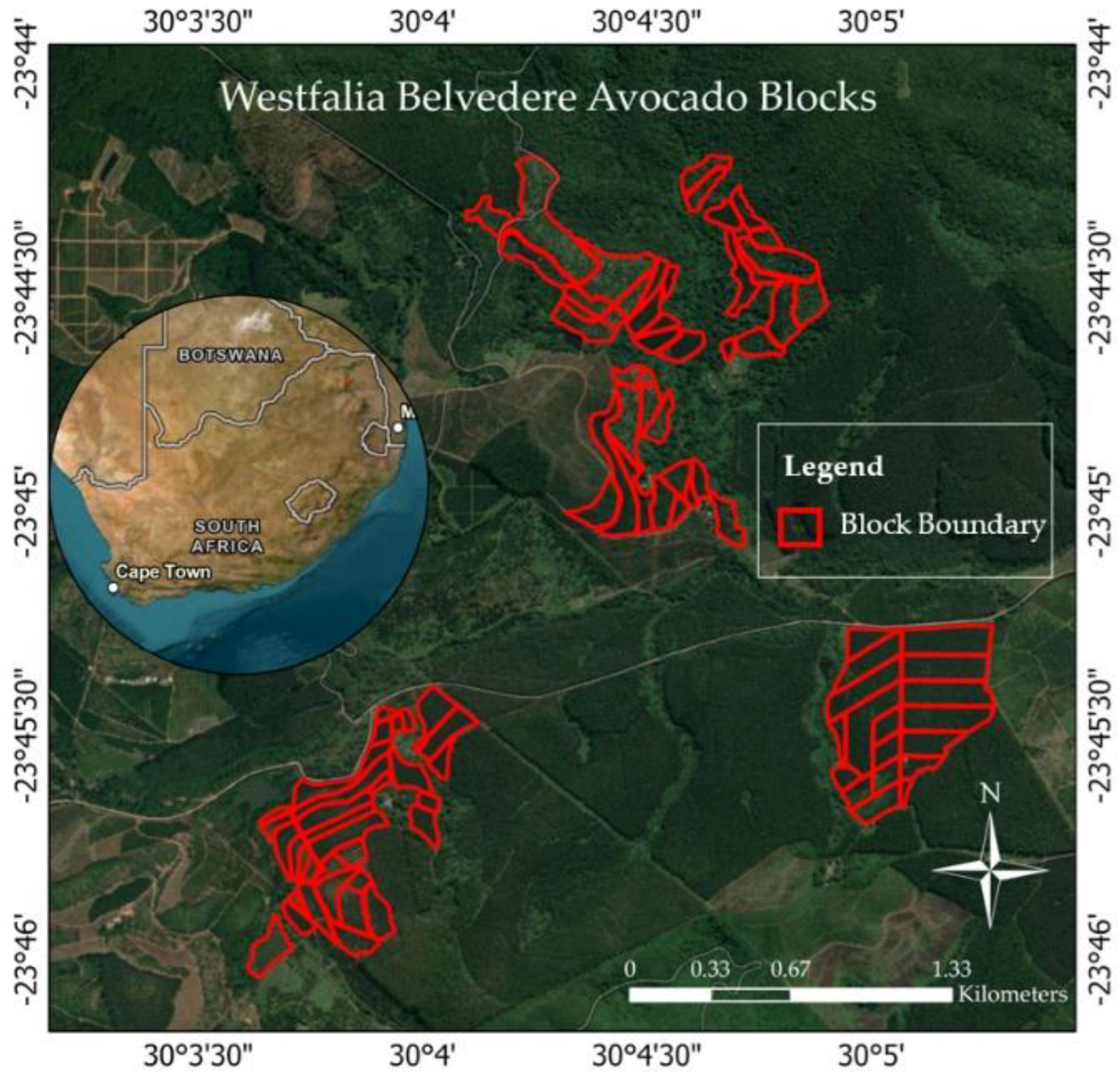
2.1. Study Area

This study was conducted in the Belvedere avocado orchards part of Westfalia Fruit Estates (Pty) Ltd, located in Tzaneen, a prominent agricultural region in the Limpopo Province of South Africa (Figure 1). The predominant avocado variety cultivated in the orchards is Hass. However, to enhance cross-pollination and ensure consistent fruit set, additional varieties such as Fuerte and Ryan are also planted in selected rows or sections within some orchard blocks. Geographically, the area lies approximately between latitudes 23.70°S and 23.78°S and longitudes 30.05°E and 30.10°E. Tzaneen is known for its favorable humid subtropical climate conditions for subtropical crops, particularly avocado and citrus, due to its fertile soils, adequate rainfall, and suitable climate [4,49].
The region experiences a subtropical climate characterized by warm, wet summers and mild, dry winters. The average annual temperature ranges between 15°C and 28°C, with peak summer temperatures reaching up to 35°C. The mean annual rainfall varies between 800 mm and 1,200 mm, mostly concentrated between October and March. The dominant soil types are deep, well-drained Ferralsols and Acrisols, which provide suitable conditions for perennial crops [49,50]. The four main climate variables used in this study, mean monthly maximum temperature (Tmax, °C), mean monthly minimum temperature (Tmin, °C), mean monthly vapor pressure deficit (VPD, kPa), and mean monthly precipitation (mm) from 2017 to 2024 are shown in Figure 2.

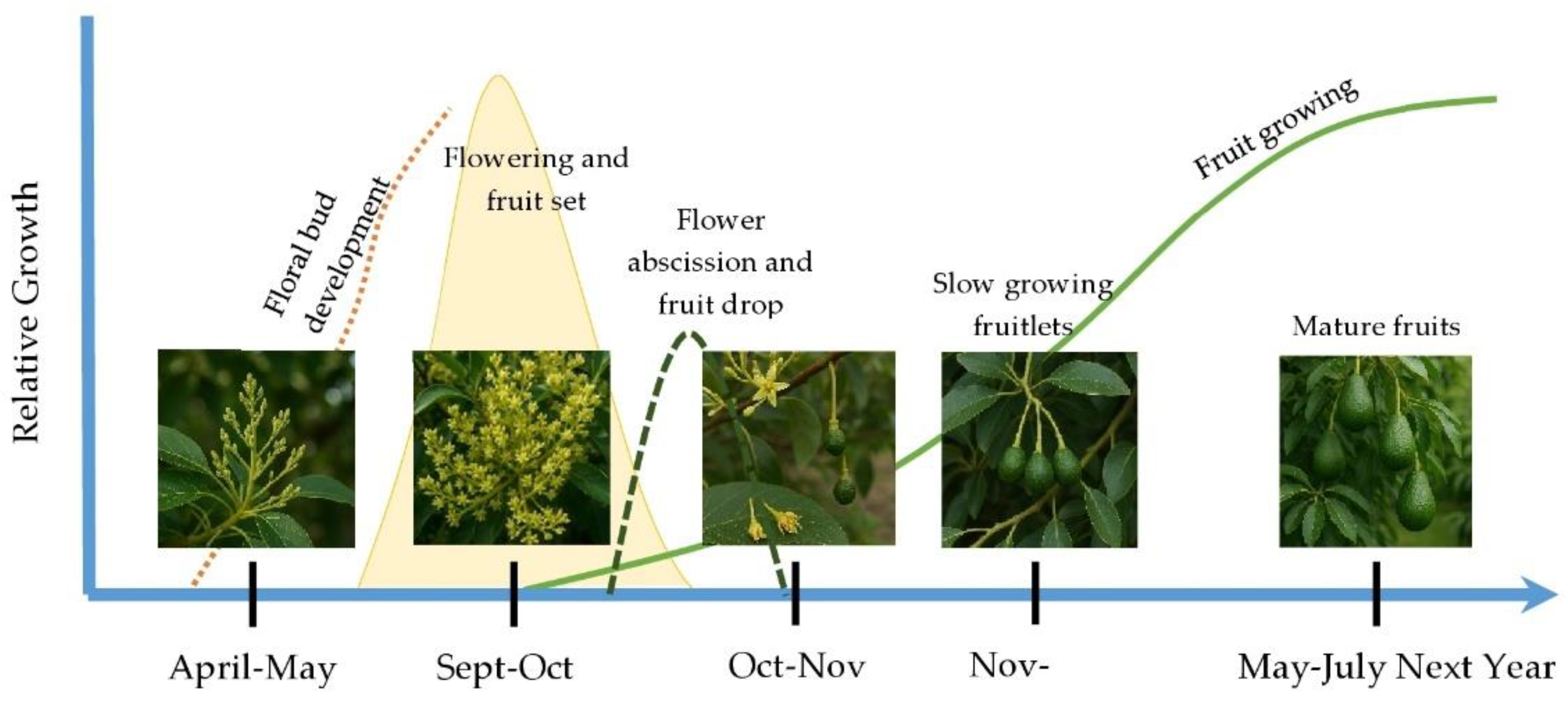
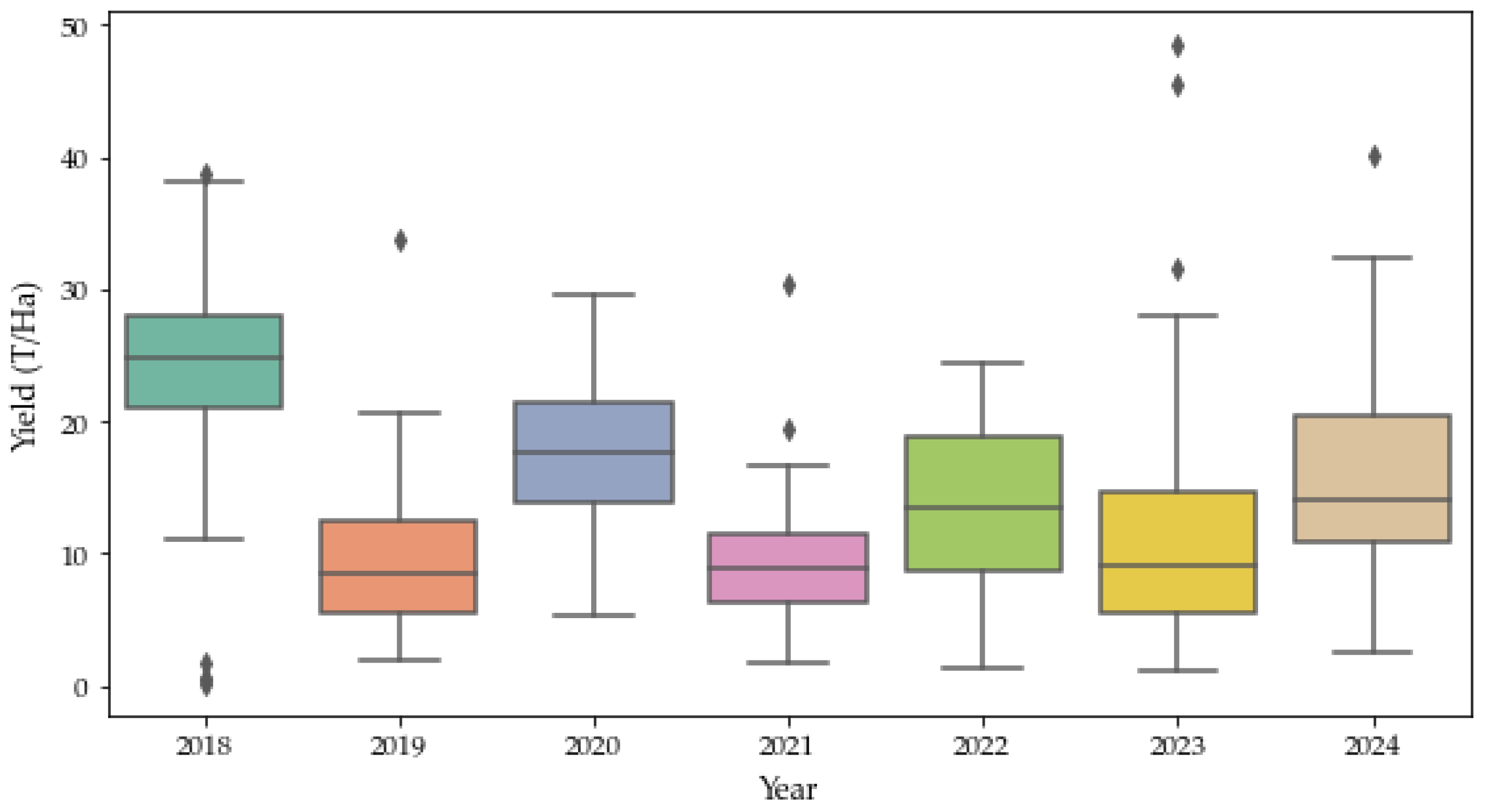
2.2. Avocado Phenology, Historical Yield and Alternate Bearing

The general phenological information of the avocado crops in Belvedere orchards in Tzaneen, South Africa was obtained from Westfalia Fruit Estates (Pty) Ltd. Avocado trees in the region typically follow a phenological cycle that begins with floral bud development in April-May, flowering and fruit set in late winter to early spring (August to September), followed by early fruit development in spring (October to November). A significant early fruit drop is observed around November – December (Figure 3). Fruit development continues through summer, with harvesting occurring from April to July depending on the cultivar and market conditions [6,13,51].
Historical avocado block yield data (T/ha) from 2018 to 2024 of 46 orchard blocks from Belveder farm, along with detailed farm maps delineating block boundaries, avocado varieties, planting year, and block area (ha), were obtained from Westfalia Fruit Estates (Pty) Ltd. The variation of yield in different seasons are shown in Figure 4. The yield distribution pattern is clearly showing an AB pattern in Belvedere farm in different seasons.
To facilitate the prediction of AB patterns in avocado orchards, annual yield records (t/ha) at the block level were used to classify each crop year as either an “on” year or “off” year. This binary classification enabled the development of supervised ML models using satellite derived VIs and FIs, and climate variables.
Traditionally, the Alternate Bearing Index (ABI), commonly defined as:
ABI   =   ( Year   1   Yield   -   Year   2   Yield ) ( Year   1   Yield +   Year   2   Yield )
ABI is widely used to quantify the degree or tendency of yield fluctuation between two successive years in an orchard. However, it does not indicate whether the upcoming year is becoming an “on” year or “off” year for any specific orchard.
To address this, a simplified thresholding method was adopted. For each orchard block, the median annual yield across all available years was computed. Each year was then assigned a binary label based on this block-specific average:
  • Years with yield greater than or equal to the median were labeled as “on” year;
  • Years with yield less than the median were labeled as “off” year.
This approach defines yields above the long-term median as biologically productive phases “on” year and yields below the median as recovery phases “off” year typically linked to AB. The use of the median, rather than the mean, provides a statistically robust threshold that is less sensitive to outliers. Consequently, this method minimizes the influence of sudden yield spikes or declines in individual years, ensuring a more stable and representative classification of long-term cropping patterns. The resulting binary labels served as the target variable for the supervised ML models developed in this study

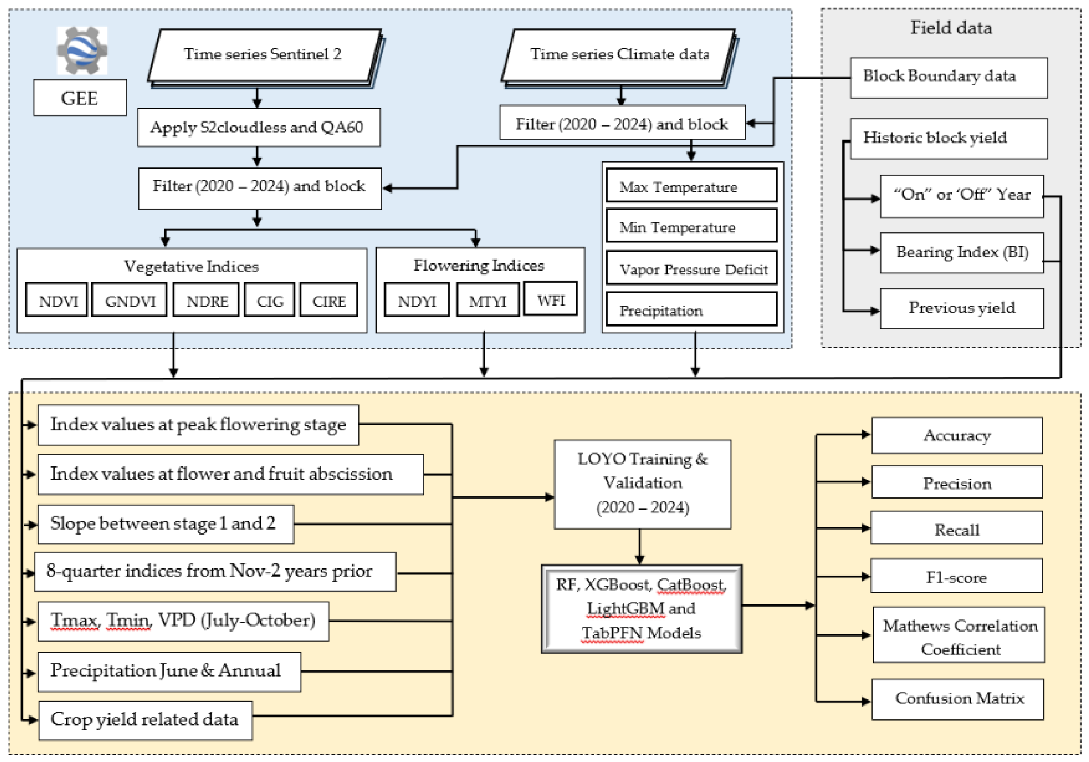
2.3. Sentinel 2 Data Acquisition and Spectral Indices

Harmonized Sentinel-2 Level-2A surface reflectance imagery was obtained through the Google Earth Engine (GEE), a cloud-based platform that enables efficient processing and analysis of multi-temporal remote sensing datasets [52]. Sentinel-2 imagery from both S2A and S2B satellites provides a high temporal resolution (5-day revisit) and spatial resolution of 10 - 20 meters, making it suitable for detecting vegetation dynamics at the orchard-block level. Data were acquired for the period from January 2016 to December 2024, encompassing multiple growing seasons of the Belvedere avocado farm. To minimize cloud contamination, the images were filtered using a cloud probability threshold (<5%), and the s2cloudless algorithm was applied for additional cloud and cloud shadow masking. Spatial filtering was performed by uploading orchard block boundary shapefiles provided by the Westfalia Fruit Estates (Pty) Ltd. into GEE Assets. Each image in the time series was clipped to individual orchard blocks, allowing for block specific analysis. These shapefiles also included metadata such as cultivar type, planting year, and block area (in hectares). From the cloud-masked Sentinel-2 imagery, a time series of ten VIs and FIs was calculated for each image date across all orchard blocks in GEE using band-specific formulas derived from Sentinel-2 reflectance values. These indices were chosen to capture both canopy vigour and flowering related spectral indices that are potentially associated with AB behaviour in avocado trees. Although several VIs exhibited high pairwise correlations, they were retained, since ensemble tree algorithms used in this study are inherently capable of handling correlated predictors and may extract distinct nonlinear relationships from redundant features.

2.3.1. Vegetation and Flowering Indices for Bearing Status Classification

The list of indices used in this study is given in Table 1 below.

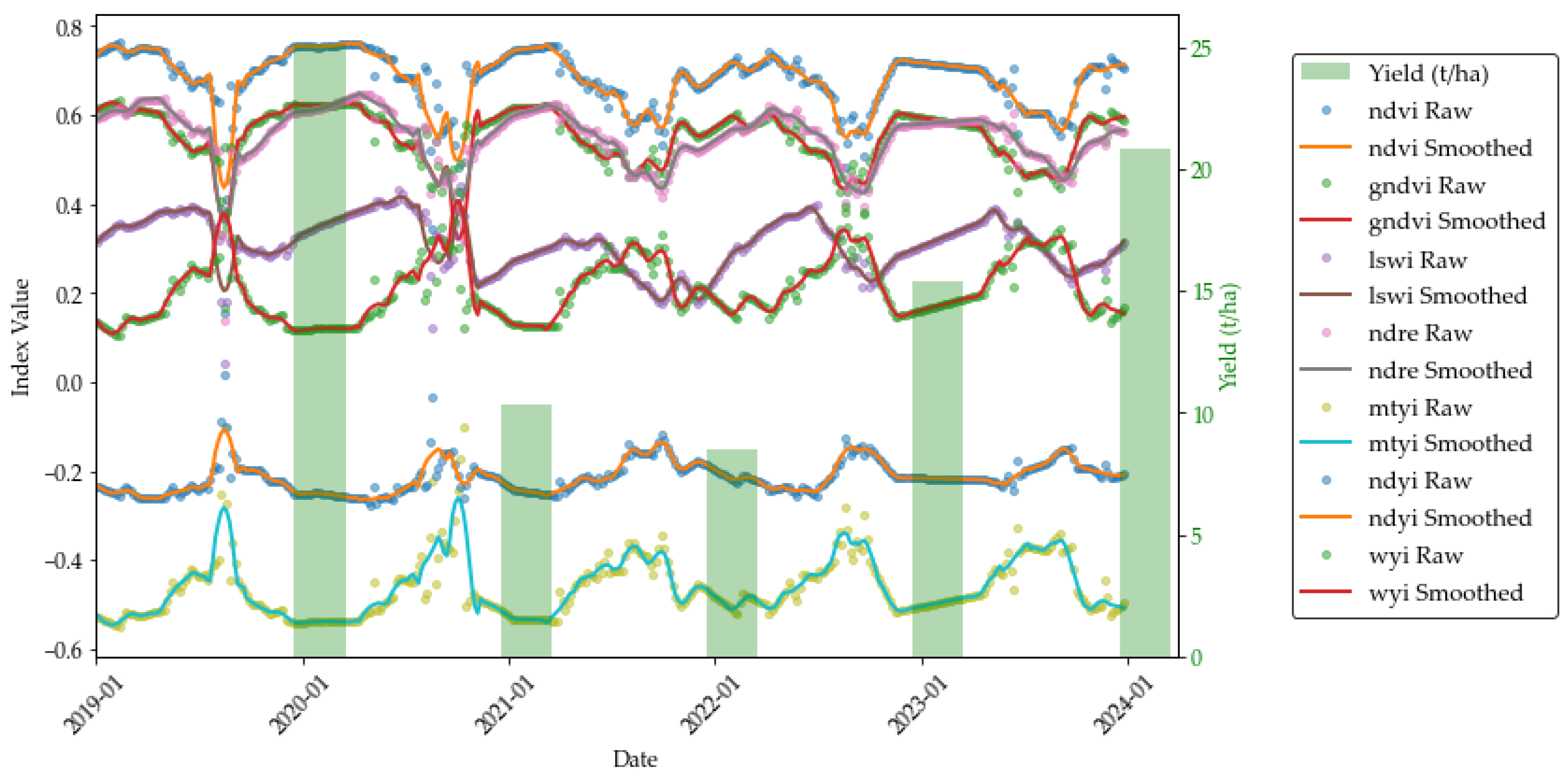
2.3.2. Savitzky-Golay Smoothing

Time-series data derived from satellite imagery are often affected by atmospheric conditions, cloud and cloud shadow cover, and residual noise, which can obscure true vegetation dynamics. To address this, the Savitzky–Golay (SG) filter was applied to smooth each time series VIs and FIs. The SG filter is a polynomial based convolution technique that performs a local least-squares regression within a moving window to reduce noise while preserving the shape and temporal structure of the original signal [59].
This method fits a low-degree polynomial to subsets of the data across a defined window, enabling the retention of key phenological features such as peaks and inflection points. The general form of the SG smoothing equation is:
Y j * =   1 N i = m i = m C i Y j 1 ,
where, Y is the original VIs value, Y* is the smoothed VIs or Fis value, Ci is the coefficient for the ith VIs or Fis value of the filter (smoothing window), N is the number of convoluting integers, which is equal to the smoothing window size (2m+1), and j is the running index of the original ordinate data table.
In this study, the smoothing parameters were set as m=5 (corresponding to an 11-point window) and a polynomial degree d=3. These parameters were selected to balance noise reduction and signal fidelity. The resulting smoothed VIs time series, sampled at a 5-day interval to match the Sentinel-2 revisit cycle, was used in all subsequent analyses to improve phenological characterization and model accuracy.

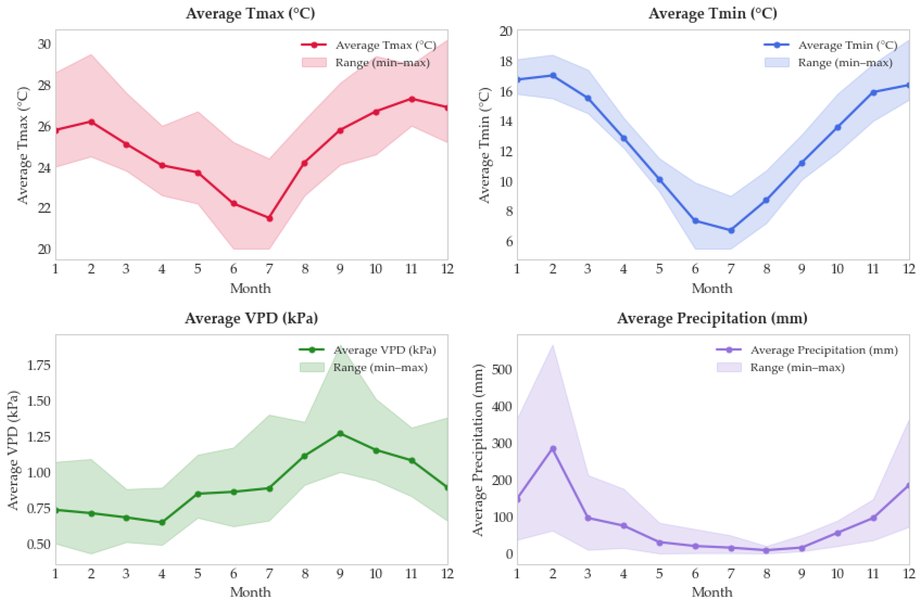
2.4. Climate Data Acquisition

In this study, monthly climate variables were acquired from the TerraClimate dataset [60] through the Google Earth Engine (GEE) platform [52]. TerraClimate is a high-resolution (~4 km) global dataset that provides monthly climate and water balance variables from 1958 onward, developed by integrating high resolution climatological normal (https://www.climatologylab.org/terraclimate.html) with time-varying reanalysis and observational data. This approach ensures both spatial and temporal consistency, making TerraClimate widely applicable in agricultural, hydrological, and ecological research [60]. For the defined study region and period, mean monthly maximum temperature (Tmax, °C), mean monthly minimum temperature (Tmin, °C), mean monthly vapor pressure deficit (VPD, kPa), and mean monthly precipitation (mm) were extracted using GEE (Figure 5). The cloud-based infrastructure of GEE facilitated efficient data access and processing without reliance on local storage or high-performance computing resources. Monthly aggregation was applied to align with crop growth cycles and phenological stages, improving the suitability of the data as ML model input variables. This integration provided reliable climate inputs, enabling consistent assessment of environmental variability and its effects on understanding AB of avocado crops.

2.5. Model Development

The methodology of data processing, feature extraction, model development and model evaluation are shown in the flow chart in Figure 6.

2.5.1. Feature Engineering of Vegetation and Flowering Indices as Well as Climate Variables

The AB in avocado is strongly associated with flowering dynamics and the early abscission of flowers or fruitlets. Previous studies have demonstrated that during “off” years, trees may exhibit normal flowering; however, low fruit set and elevated abscission rates largely driven by hormonal imbalances and restricted carbohydrate reserves contribute to reduced yields [28,61]. Building on this physiological basis, the present study incorporated flowering sensitive indices as a novel and scalable approach for detecting reproductive signals that are critical to predicting AB.
To extract phenologically relevant information, Savitzky–Golay smoothed time series of VIs and FIs were processed to derive three temporal metrics, which could be potential drivers of AB:
  • Peak Bloom Stage (August–September) – Maximum values of FIs and minimum values of VIs were extracted, corresponding to the stage of highest flower intensity and lowest vegetative dominance in the study area [29].
  • Early Fruit Drop (7–8 weeks after peak flowering) – Minimum values of FIs and maximum values of VIs were computed, reflecting the period when abscission processes are most pronounced and vegetative recovery is underway.
  • Temporal Gradient – The rate of change between the two above stages was calculated to capture sharp declines in FIs or distinct peaks in VIs, serving as strong indicators of “on” or “off” years.
In addition to these phenological metrics, all VIs and FIs were aggregated over the preceding eight quarters (three-month intervals) starting from November of the two prior years. This long-term temporal information enabled the incorporation of lagged effects from prior flowering and fruiting cycles, which are well-documented drivers of AB behavior.
The monthly climate variables (Tmax, Tmin, VPD and precipitation) were systematically correlated with historical yield records to identify critical periods influencing avocado productivity. The analysis revealed that the months from June to October exhibited the strongest associations with yield variation and were therefore selected as key climatic predictors for inclusion in the ML model development.
Finally, these engineered features were integrated with historical yield records (T/Ha) from previous two years and the ABI from previous year, to provide a comprehensive feature space for ML model development. The combined dataset thus captured spectral dynamics, flowering intensity, fruit abscission patterns, canopy vigour, and yield fluctuations allowing a multidimensional understanding of the drivers of AB in avocado production systems.
Feature scaling was performed using the StandardScaler function in scikit-learn, standardizing continuous variables to a mean of zero and a standard deviation of one. Although tree-based models are generally scale-invariant, standardization ensured numerical consistency and reproducibility across datasets. The scaler was fitted on the training data and applied to the test data to prevent data leakage and maintain model integrity.
Since the number of “on” and “off” year observations varied across years, the dataset exhibited class imbalance in the target variable. To address this and minimize bias in model training, the Synthetic Minority Over-sampling Technique (SMOTE) was applied to balance the classes. SMOTE creates synthetic samples of the minority class by interpolating between existing instances, thereby improving representation and model generalization [62]. This approach, increasingly used in agricultural studies [63], ensured adequate representation of both “on” and “off” year patterns, providing a balanced and reliable foundation for ML model development.

2.5.2. Machine Learning Model Algorithms

To classify AB patterns in avocado orchards, we evaluated five supervised ML algorithms, all implemented using the Scikit-Learn [64] and XGBoost [42] libraries in Python.
  • Random Forest (RF): RF is an ensemble classifier that constructs multiple decision trees through bootstrap aggregation [65]. Predictions are derived via majority voting across trees, providing resilience against overfitting and robustness in handling noisy, multicollinear datasets. For this study, the number of trees (n_estimators), maximum tree depth, and minimum samples per split were optimized using cross-validation.
  • Extreme Gradient Boosting (XGBoost): XGBoost implements gradient boosting with enhanced computational efficiency and regularization[42]. It builds trees sequentially, where each subsequent tree reduces the residual errors of the ensemble. Critical hyperparameters included learning rate, maximum tree depth, subsample fraction, and number of boosting iterations.
  • Categorical Boosting (CatBoost): CatBoost extends gradient boosting by incorporating ordered boosting to mitigate overfitting and reduce prediction shift [43]. While originally designed for categorical feature handling, in this study it was applied exclusively to continuous predictors. Hyperparameters such as learning rate, tree depth, and number of iterations were tuned using grid search.
  • Light Gradient Boosting Machine (LightGBM): LightGBM employs histogram-based feature binning and a leaf-wise growth strategy with depth constraints [44]. These optimizations accelerate training while reducing memory usage. Tuning parameters included number of leaves, maximum depth, feature fraction, and learning rate.
  • Tabular Prior Data Fitted Network (TabPFN): TabPFN is a transformer-based neural network trained on millions of synthetic datasets, approximating Bayesian inference for tabular data classification [45]. Unlike conventional algorithms, TabPFN requires minimal parameter adjustment and leverages prior knowledge to achieve strong generalization. In this study, the pretrained TabPFN model was directly applied without additional tuning.

2.5.3. Training and Validation Strategy

Leave-One-Year-Out (LOYO) Cross-Validation
A Leave-One-Year-Out (LOYO) cross-validation approach was adopted to evaluate temporal generalization. In each iteration, data from a single year were withheld as the test set, while models were trained on all remaining years. This process was repeated until each growing season (2020–2024) had served once as the validation fold.
LOYO validation is particularly well-suited for AB studies because it ensures strict temporal independence between training and testing. By preventing leakage of information across years, LOYO better represents operational conditions, where the goal is to predict bearing status of a forthcoming season using only historical data.
Hyperparameter Tuning of Machine Learning Models
For RF, XGBoost, CatBoost, and LightGBM, hyperparameters were optimized using a grid search approach combined with five-fold internal cross-validation within each training fold. The optimal settings were determined based on the F1-score, which provides a balanced measure of precision and recall and is particularly suitable for binary imbalanced datasets.
TabPFN was implemented using its default pretrained configuration, thereby eliminating the need for hyperparameter optimization while leveraging its transformer-based prior-fitting architecture.
The optimal hyperparameter configurations for each model are summarized in Table 2.

2.5.4. Model Evaluation Metrics

To assess the performance of ML classification models in identifying AB patterns in avocado orchards, specifically distinguishing “on” year (labeled as 1) from “off” year (labeled as 0), a set of widely accepted evaluation metrics was applied. These metrics offer a comprehensive view of each model’s predictive accuracy, reliability, and overall robustness within a binary classification context. Central to this assessment is the confusion matrix, which summarizes the model’s predictions by categorizing them into four key components: true positives (TP), true negatives (TN), false positives (FP; Type I error), and false negatives (FN; Type II error). This framework enables a detailed analysis of classification outcomes and supports the computation of various performance measures such as accuracy, precision, recall, and F1-score. The following metrics were used:
  • Accuracy: Accuracy measures the overall correctness of the model, defined as the ratio of correctly predicted observations to the total number of observations:
Accuracy = TP + FP TP + FP + TN + FN
While accuracy provides a general sense of model performance, it can be misleading in imbalanced datasets [66].
2.
Precision: Precision quantifies the proportion of positive predictions that are actually correct. It is especially important when the cost of false positives is high.
Precision = Tp TP + FP
High precision indicates a low false positive rate, which is critical when predicting "on" bearing years in agriculture, where resource misallocation could occur due to misclassification.
3.
Recall (Sensitivity or True Positive Rate): Recall indicates the proportion of actual positive cases that were correctly identified by the model:
Recall = TP TP + FN
A high recall ensures that most of the "on" bearing years are detected, minimizing false negatives and ensuring that productive seasons are not overlooked [67].
4.
F1-Score: The F1-score is the harmonic mean of precision and recall and is a balanced metric for evaluating classification performance when classes are imbalanced:
F 1 - score = 2   ×   Precision   ×   Recall Precision + Recall
F1-score is particularly useful when both false positives and false negatives are costly, as is often the case in phenological studies involving crop yield prediction [68].
5.
Matthews Correlation Coefficient (MCC): The Matthews Correlation Coefficient (MCC) is a comprehensive statistical metric that evaluates the quality of binary classifications by considering true and false positives and negatives. It is defined as:
MCC = TP × TN - ( FP   × FN ) ( TP + FP ) ( TP + FN ) ( TN + FP ) ( TN + FN )
MCC returns a value between −1 and +1, where +1 indicates perfect prediction, 0 represents random performance, and −1 corresponds to total disagreement between predictions and observations. Unlike accuracy or F1-score, MCC remains robust even with highly imbalanced datasets, providing a balanced measure of model performance across both classes (Chicco & Jurman, 2020). This makes it particularly valuable in agricultural modelling and remote sensing applications where class imbalance, such as between “on” and “off” bearing years of avocado crop is common.
6.
Confusion Matrix: The confusion matrix provides a detailed breakdown of predicted versus actual classes, helping to visualize classification errors:
Predicted Positive Predicted Negative
Actual Positive True Positive (TP) False Negative (FN)
Actual Negative False Positive (FP) True Negative (TN)
This matrix supports a deeper understanding of model behavior and error types in each class.
7.
Receiver Operating Characteristic (ROC) Curve and Area Under the Curve (AUC): The ROC curve plots the true positive rate (recall) against the false positive rate across various threshold settings. The AUC quantifies the model's ability to distinguish between classes:
  • An AUC of 1.0 indicates perfect classification.
  • An AUC of 0.5 suggests no discriminative power.
ROC-AUC is threshold-independent and provides a more nuanced evaluation of classifier performance over multiple thresholds [69].

2.5.5. Model Interpretation

Model interpretability was prioritized to link predictions with physiological and climatic drivers of AB. For RF, XGBoost, CatBoost, and LightGBM, permutation feature importance was calculated by measuring the reduction in predictive accuracy when each variable was randomly permuted.
For TabPFN, Shapley Additive Explanations (SHAP) values were computed (Lundberg & Lee, 2017). SHAP analysis decomposed each model output into additive feature contributions, thereby quantifying both the magnitude and direction of influence of individual variables.
This interpretability framework highlighted the importance of FIs (WYI, MTYI) and key climate variables (Tmax, VPD), consistent with known biological mechanisms driving carbohydrate partitioning and resource stress in avocado trees.

2.5.6. Computational Environment

All analyses were conducted in Python 3.10. The following libraries were employed: scikit-learn (RF), xgboost (XGBoost), catboost (CatBoost), lightgbm (LightGBM), and tabpfn (TabPFN). Model interpretability was implemented using the shap package. Sentinel-2 preprocessing and index computation were performed in GEE, while figure generation was carried out using matplotlib and seaborn libraries.

3. Results

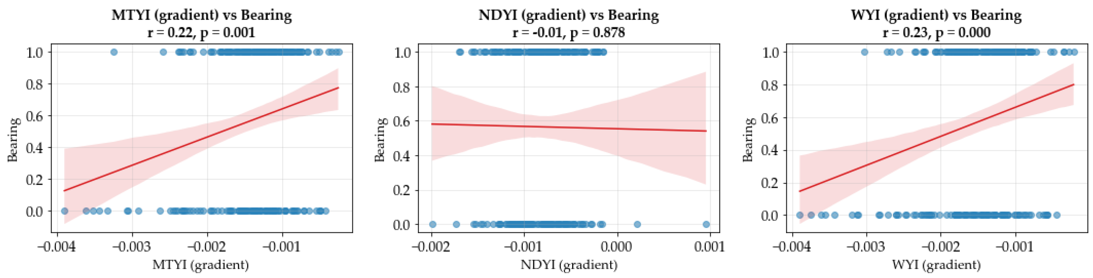
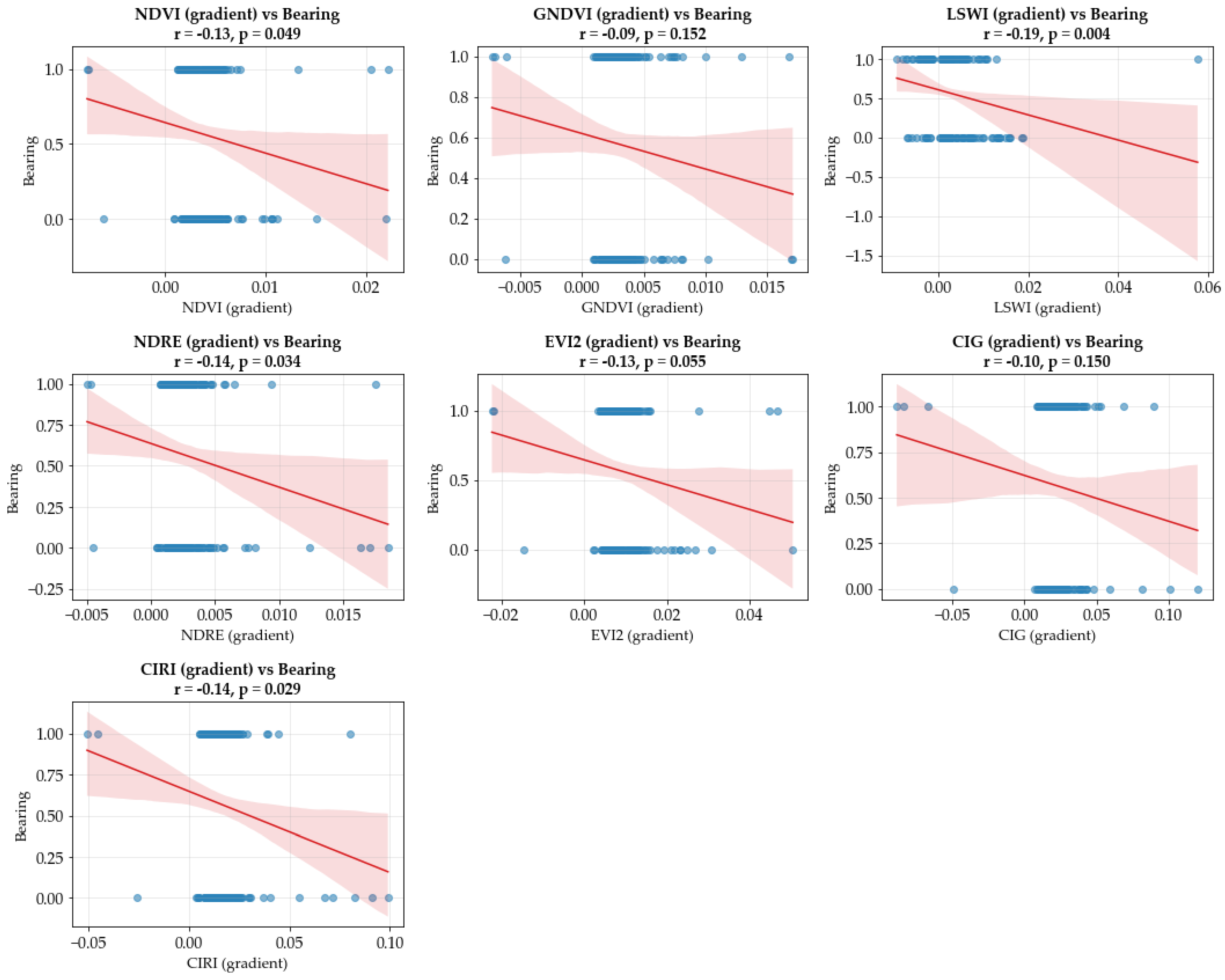
3.1. Temporal Dynamics of Vegetation and Flowering Indices

To characterize the flowering patterns and overall phenology of avocado trees in relation to the subsequent yield or AB, time-series data for seven VIs and FIs (all with values below 1.0 for visibility in the graph) are presented for an example block (‘Block 42’) in Figure 7. The temporal profiles of smoothed VIs and FIs values using the Savitzky–Golay filter and historical annual yield data in different years are also overlayed in the figure. The Sentinel-2 derived VIs and FIs exhibited distinct seasonal trends that aligned with the phenological cycle of avocado trees. The FIs (WYI, NDYI and MTYI) demonstrated clear and consistent peaks between August and September across most years, corresponding with known flowering periods for avocado in Tzaneen, whereas VIs showed a contrasting trend. During peak flowering months, NDVI, GNDVI, LSWI and NDRE tended to exhibit troughs, indicating a temporary reduction in canopy greenness due to the shift from vegetative to reproductive growth. These indices gradually increased following the flowering period, aligning with new leaf flushes and fruit development stages. One notable observation is the absence of a consistent relationship between peak FIs and yield. Years with strong peaks in FIs did not necessarily correspond to higher yields or “on” years, suggesting that early-season flowering intensity alone is not a reliable indicator of final production.
To gain deeper insight into flowering dynamics, the FIs values during the peak flowering period and their relationship with bearing status over the five-year study period (2020–2024) are presented in Figure 8. All three FIs exhibited weak negative correlations (R = - 0.06, - 0.03, and - 0.06, respectively) with p > 0.33, indicating that profuse flowering does not necessarily result in higher yields, which is consistent with the findings of Garner and Lovatt (2008).
The relationship between the temporal gradient of FIs from peak flowering to early fruit drop and bearing status is presented in Figure 9. Notably, MTYI and WYI exhibited steeper gradients during high-yielding “on” years compared to low-yielding “off” years. This indicates reduced flower and fruit abscission in on-years relative to off-years, highlighting the potential of these gradients as early indicators for predicting AB. However, NDYI didn’t show a significant correlation with r = -0.01.
An opposite trend of temporal gradient was observed between peak flowering and early fruit drop with bearing status for all seven VIs (Figure 10). In contrast to FIs, VIs (NDVI, GNDVI, LSWI, NDRE, EVI2, CIG, and CIRE) exhibited lower gradients during high-yielding “on” years compared to low-yielding “off” years. This pattern indicates that canopy vigour and greenness remain relatively stable in “on” years, with less pronounced temporal changes between peak flowering and early fruit drop.
Higher correlation coefficients (R) were found for the gradient of LSWI, CIRE, and NDRE (R = −0.19, −0.14, and −0.14 respectively), suggesting stronger negative relationships with AB patterns. These indices are sensitive to canopy water status and chlorophyll/nitrogen content, reflecting physiological constraints, such as water stress and nutrient depletion that contribute to flowering and fruit abscission, and ultimately lower yield in “off” years. The reduced gradients of all VIs in “on” years likely reflect minimal fruit drop and a steady accumulation of fruit set, whereas higher gradients in off years suggest greater fluctuations in canopy condition, potentially due to flower and fruit abscission. These results imply that low VIs gradients may serve as early indicators of stable canopy function associated with high yields, complementing the predictive insights provided by Fis.
The rank order of correlation strengths of different VIs and FIs aggregated over the preceding eight quarters (three-month intervals) starting from November of the two prior years with AB status were presented in Figure 11. In general, the quarter 2 (February to April) of 2 prior years (q2_y2) spectral VIs and FIs showed stronger relationships with AB patterns. Here also CIRE and NDRE, which are sensitive to canopy chlorophyll/nitrogen content performed better than other indices. Other VIs and FIs in q2_y2 (GNDVI, MTYI, CIG, WYI, NDVI EVI2) showed better performance.

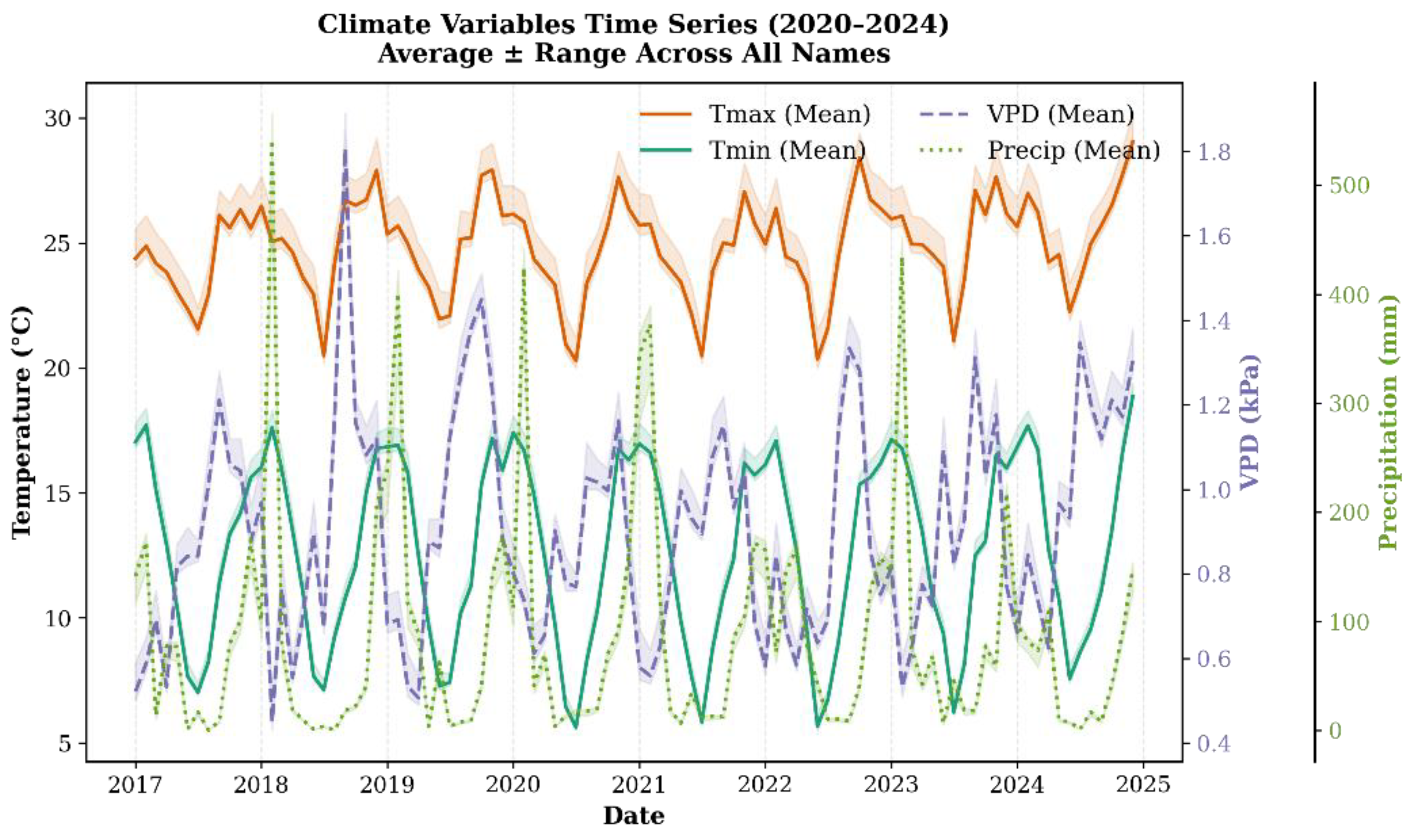
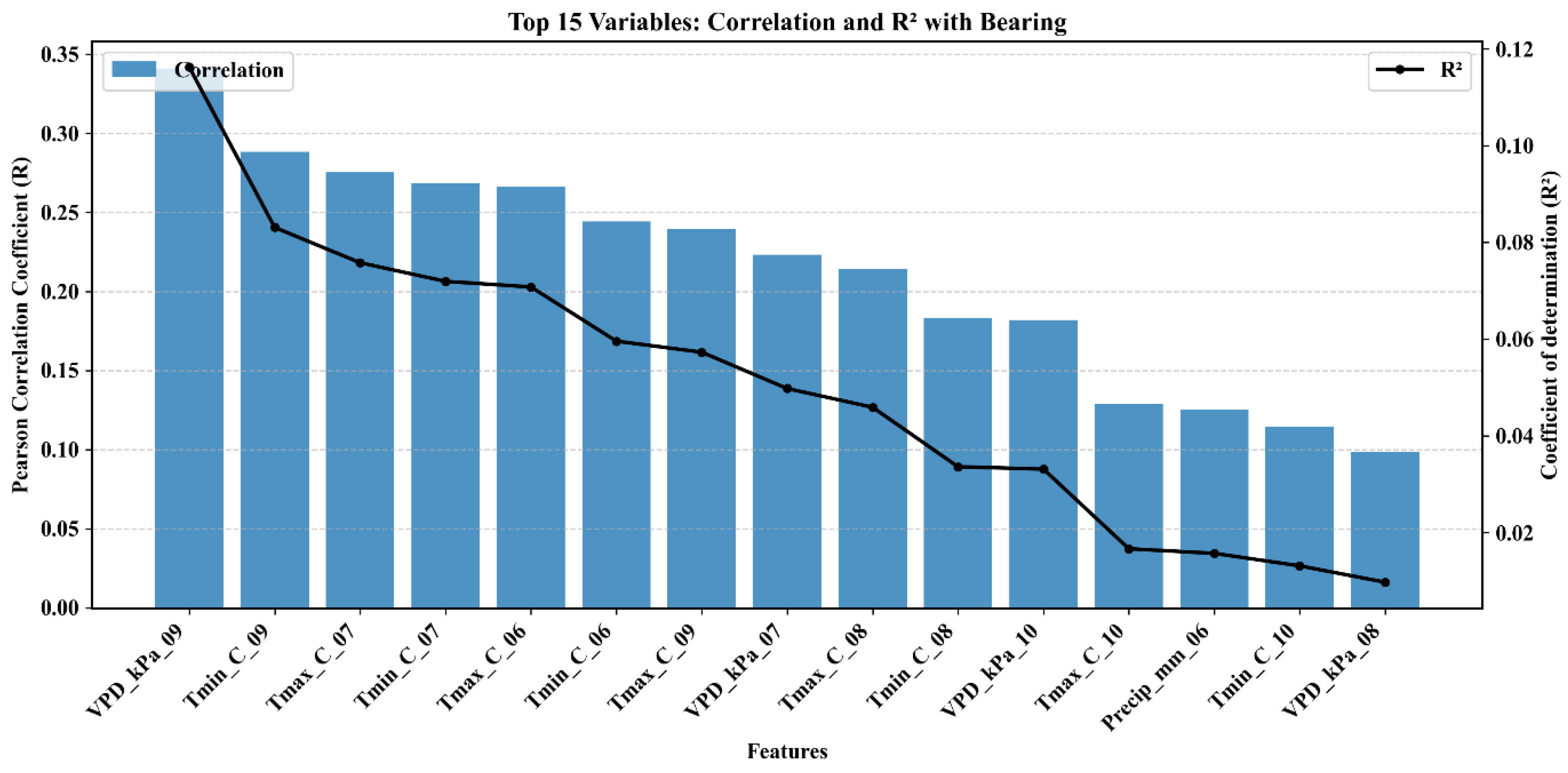
3.2. Climate Variables and Their Influence

The rank order of correlation strengths between the top 15 climate variables in different months and the bearing status in the following year is shown in Figure 12. Climate variables exerted a pronounced effect on orchard condition and bearing patterns. During peak flowering period (July to September), VPD, Tmin and Tmax showed a greater influence in bearing pattern of following year compared to other months.
The correlation of top 8 climate variables with bearing status is shown in Figure 13. The VPD during September, peak flowering period in the study region, when Tmax varies from 24 to 28 °C, showed a profound influence (R = 0.34) on high yielding or “on” year with VPD ranging from 1.0 to 1.85. The Tmin at that time varied from 10 to 13°C (Figure 4). Tmin at the same time period and Tmax in July also showed a positive correlation with R = 0.29 and R = 0.28 respectively. Overall, the correlation of VPD, Tmax and Tmin at the time of flowering and initial fruit set suggests that the climate variables could be a potential drivers for determining upcoming season bearing status for avocado crops in the study region. Precipitation in June showed little influence on bearing status, possibly due to supplemental irrigation practices implemented by growers.

3.3. Model Performance for Alternate Bearing Classification

Model performance metrics: Accuracy, Precision, Recall, F1-score, ROC-AUC and MCC are shown in Figure 14. Among the ensemble tree-based algorithms, RF and XGBoost achieved low performance, with mean accuracies of 0.63 and 0.71 respectively. CATBoost and LightGBM produced marginally higher F1-scores of 0.74 and 0.75 respectively, likely due to their enhanced capacity to handle categorical variables and class imbalance of AB through ordered boosting and gradient-based leaf optimization.
The TabPFN model outperformed all other approaches, achieving an overall Accuracy = 0.88, F1-score = 0.88, and AUC = 0.95 across LOYO folds. This superior performance can be attributed to the probabilistic and prior-informed architecture of TabPFN, which effectively integrates complex interdependencies among vegetation, flowering, and climatic predictors. Its meta-learning capability enables rapid generalization from limited temporal data while maintaining robustness against overfitting.

3.4. Temporal Stabiligy of Models

The comparative model accuracies and inter-annual consistency of five ML models shown in Figure 15, illustrates the TabPFN’s stable predictions across all test years from 2020 to 2024. The year-wise ROC-AUC revealed that all models demonstrated higher classification accuracy during pronounced “off” years (2021 and 2023) but experienced moderate accuracy during other seasons with intermediate yields or pronounced “on” years (2020, 2022 and 2024) except RF, which performed well in “on” years compared to “off” years (Figure 3 and Figure 12). TabPFN and XGBoost displayed the most consistent performance across years, maintaining balanced ROC-AUC for classifying “on” or “off” years.
Notably, TabPFN’s robustness under LOYO validation indicates its capacity to generalize effectively under variable climatic conditions in different years. For instance, during 2021 with lower yield or “off” year, the model retained high predictive accuracy (ROC-AUC = 0.93), whereas the ensemble models exhibited comparatively lower performance. These results suggest that TabPFN better captures nonlinear interactions between environmental stressors and canopy spectral responses associated with yield fluctuations.

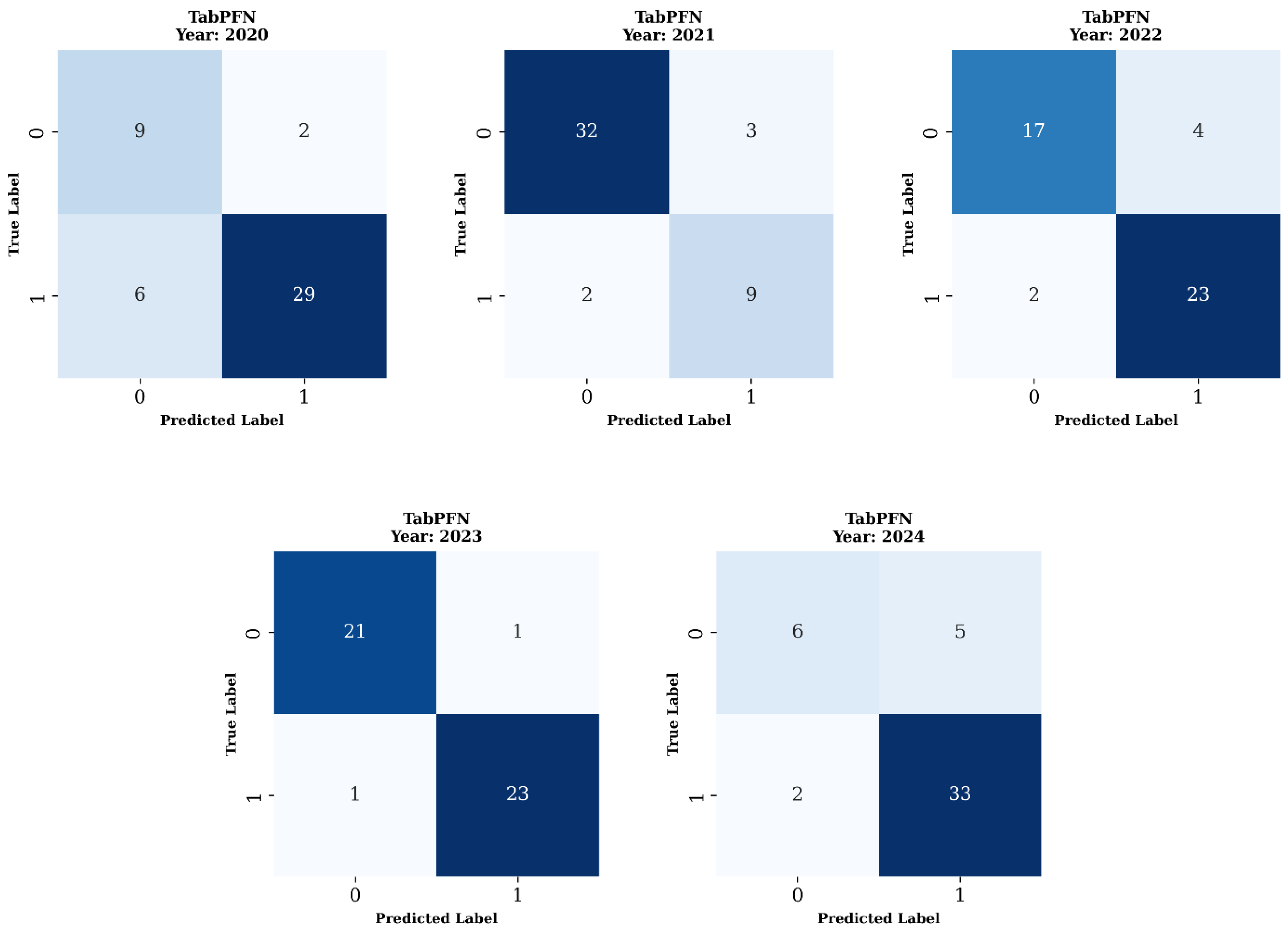
3.5. Confusion Matrix Analysis

A detailed examination of the confusion matrix (Figure 16) for the TabPFN classifier further illustrates its classification efficacy. Confusion matrix analysis revealed that TabPFN achieved balanced detection of both “on” and “off” years, with highest misclassification rates below 17%, which occurred in 2020 season. The best performed year was 2023, where, out of 46 test samples, the model correctly identified 21 “off” season samples and 23 “on” season samples. Only 1 false positive and 1 false negative were recorded, yielding a balanced error distribution. The Type I error (false positives) and Type II error (false negatives) remained minimal, supporting the model's robustness.

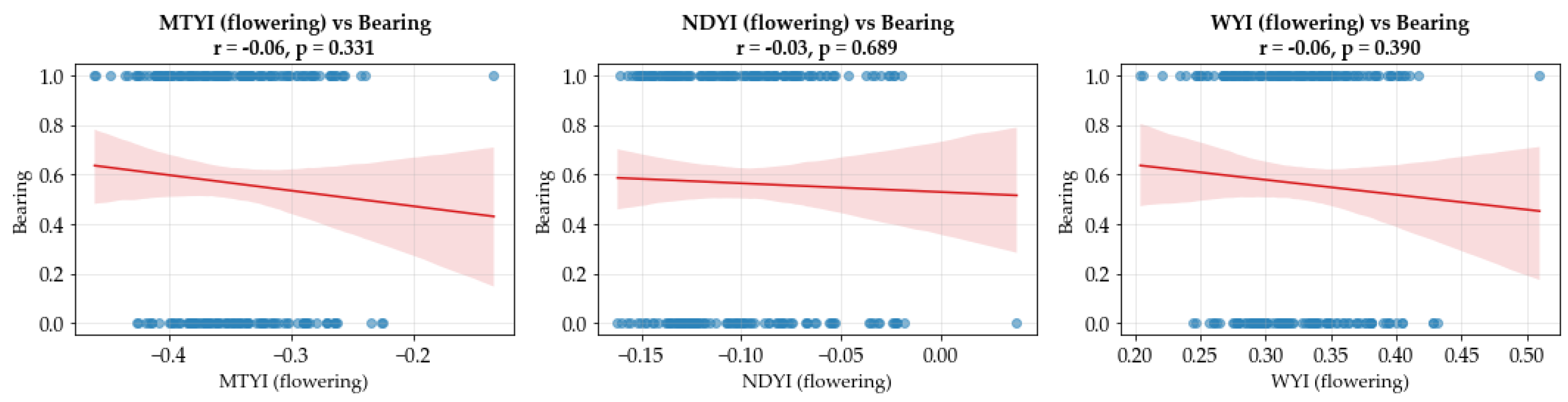
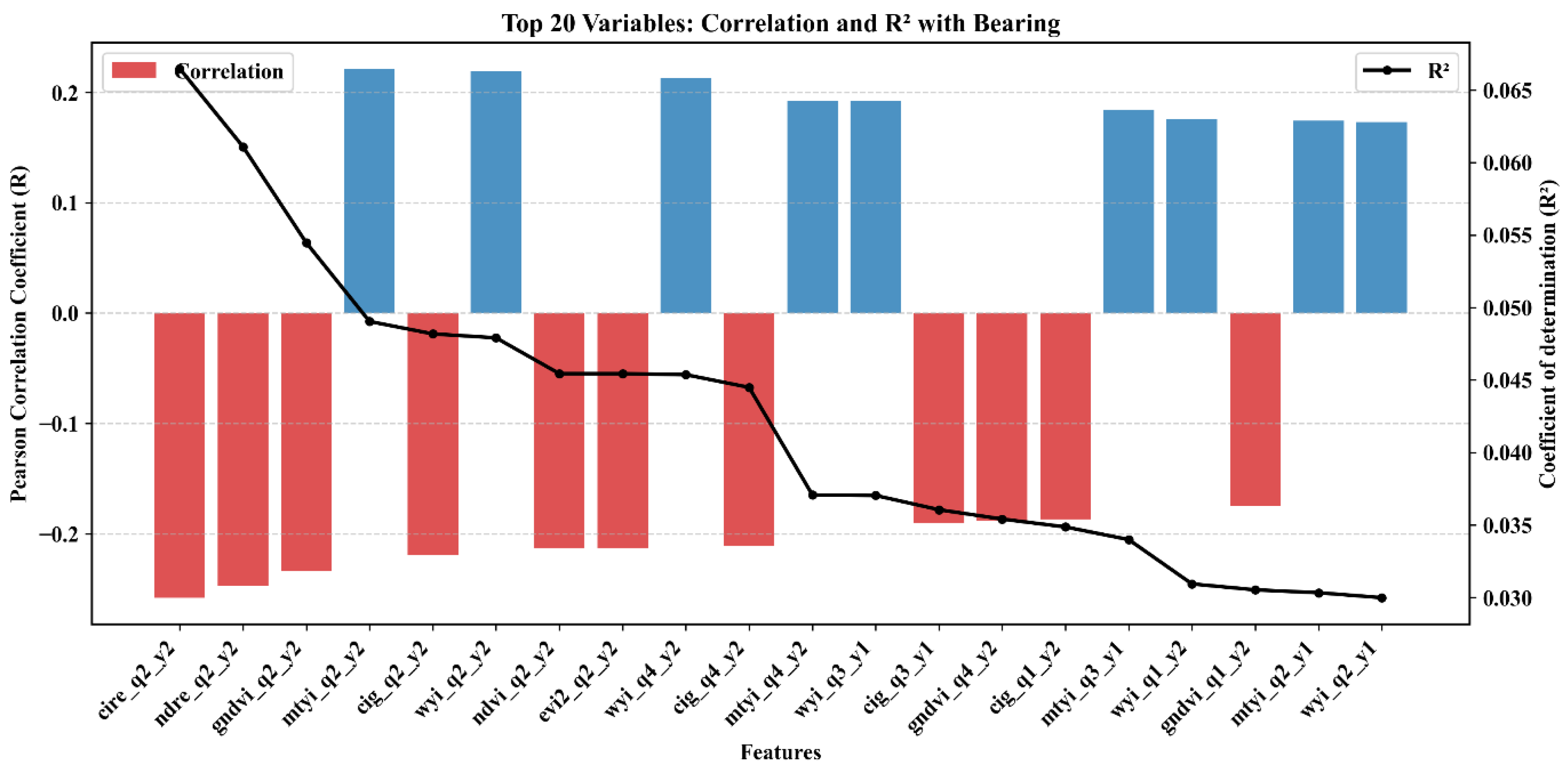
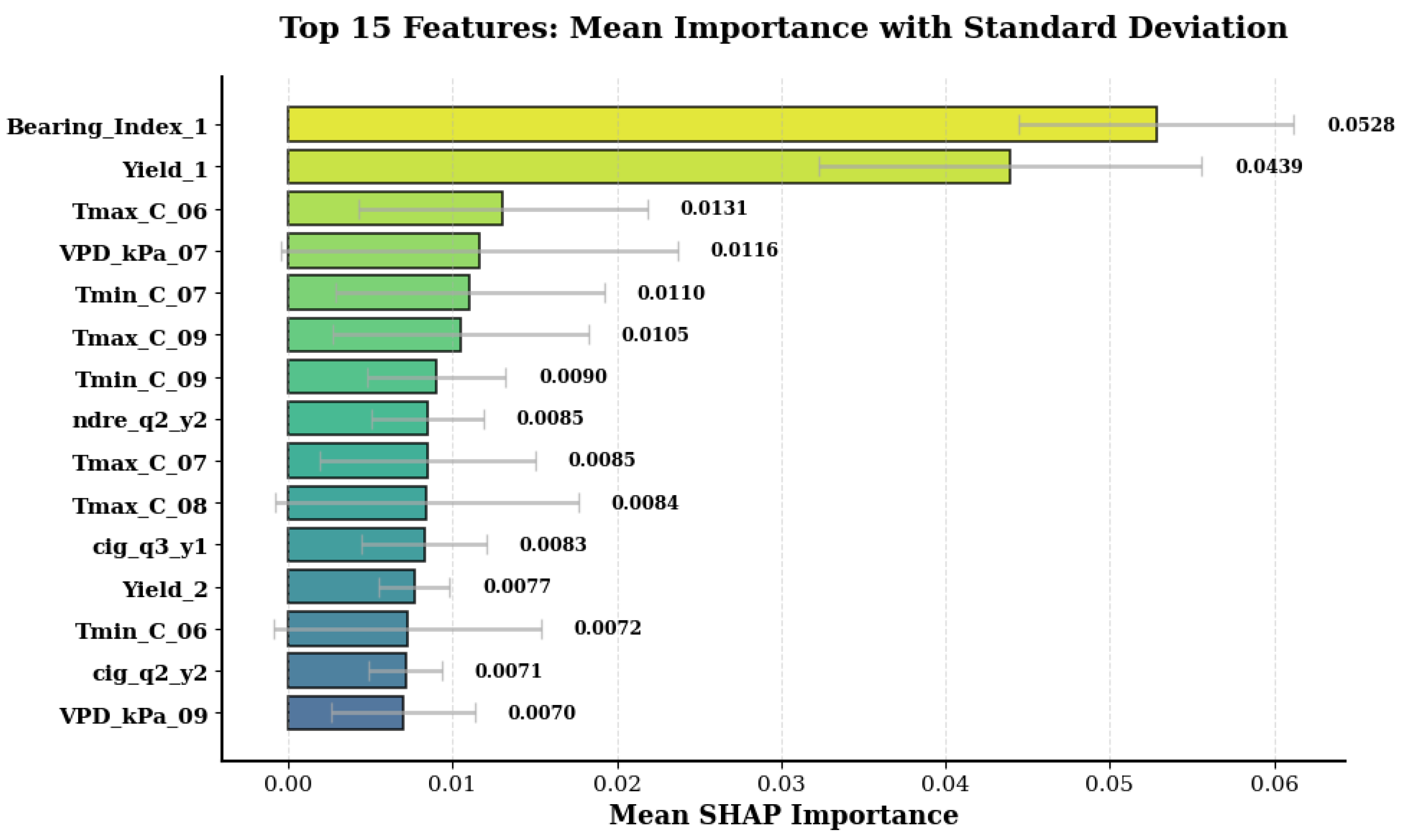
3.5. Feature Importance and Variable Contribution

Feature importance analysis (Figure 17) showed that climate variables and chlorophyll indices had the strongest influence on the model’s performance. In the TabPFN model, yield from the previous year and the bearing index were identified as two of the most important predictors of AB. The climate variables, Tmax, Tmin and VPD at the period of flowering and initial fruit set also played a major role, highlighting how weather conditions shape yield variation between years. Both chlorophyll indices, CIG and NDRE were observed as strong predictors, reflecting their link to canopy health and photosynthetic activity. These variables consistently ranked among the top features separating “on” and “off” years, confirming that both climate and physiological factors are central to AB. Overall, the results suggest that combining multiple spectral and climate variables provides a more reliable approach to predict AB.

4. Discussion

The phenomenon of AB in avocado has been widely recognised as a complex biological process influenced by both endogenous and exogenous factors [6,70]. In the present study, the integration of multi-temporal remote sensing indices and climate variables provided a comprehensive assessment of the mechanisms underlying this irregular yield pattern. The findings indicated that AB in avocado is not solely determined by the intensity of flowering but is governed by the combined influence of climatic stresses, canopy physiological responses, and post-flowering fruit retention dynamics.
Distinct seasonal patterns were observed for the VIs and FIs derived from Sentinel-2 imagery. The FIs (WYI, NDYI, and MTYI) exhibited consistent peaks between August and September, coinciding with the documented flowering period of avocado in subtropical regions such as Tzaneen. However, the magnitude of these peaks did not correspond consistently with high yields, confirming earlier observations by Garner and Lovatt [25] that excessive floral intensity does not necessarily translate into greater fruit production. It has been proposed that this discrepancy may result from the physiological trade-off between reproductive effort and subsequent fruit retention, as heavy flowering is frequently followed by extensive abscission of flowers and immature fruits [13,71]. Consequently, the quantity of flowers produced during an “on” year may not be an accurate indicator of potential yield unless environmental conditions remain favourable throughout the fruit-set period.
The analysis of temporal gradients of FIs further demonstrated that the rate of decline in index values after the peak flowering period was steeper during “on” years than during “off” years. This finding suggests that less abscission of flowers and fruitlets occurs during productive seasons. In contrast, VIs (NDVI, GNDVI, LSWI, NDRE, CIG, CIRE, and EVI2) exhibited an inverse relationship with bearing status, showing smaller gradients during “on” years and more pronounced declines during “off” years. Such behaviour is consistent with the physiological response of avocado trees under fruit-bearing stress, in which vegetative growth and canopy greenness are temporarily suppressed during heavy fruiting cycles [72]. The stability of canopy indices during high-yielding years may therefore reflect a more efficient balance between photosynthetic activity and fruit development, whereas greater fluctuations in “off” years may indicate resource reallocation to vegetative recovery.
Among the VIs, LSWI, CIRE and NDRE demonstrated the strongest negative correlation with AB status, implying that canopy water content and chlorophyll/nitrogen status play critical roles in determining the yield pattern. Similar associations between canopy water potential, nutrient status and yield variability have been reported in previous studies on avocado and other perennial fruit crops [73,74]. The results of the present analysis therefore support the hypothesis that spectral indicators of canopy physiology can serve as early indicators of forthcoming yield conditions.
Climate variables were also found to exert a decisive influence on bearing patterns. The correlation analysis revealed that vapour pressure deficit (VPD), minimum temperature (Tmin), and maximum temperature (Tmax) during the flowering period (July–September) were the most influential variables in determining the subsequent season’s yield. The positive correlation of VPD during September with bearing status suggested that moderate atmospheric demand for moisture may promote pollination efficiency and fruit set, whereas extreme VPD values could induce floral desiccation and abscission. These results are consistent with those reported by Acosta-Rangel, Li, Mauk, Santiago and Lovatt [35], who observed that climatic anomalies such as low temperature and water-deficit stress during flowering act as primary triggers for AB in avocado. The limited influence of rainfall observed in this study may be attributed to the widespread adoption of supplemental irrigation in commercial orchards, which mitigates short-term precipitation deficits.
The ML analysis provided further insight into the relative importance of the variables contributing to avocado AB classification. Among the models evaluated, the TabPFN algorithm demonstrated the highest predictive accuracy and temporal stability. This performance can be attributed to its ability to incorporate probabilistic priors and capture non-linear interdependencies between phenological, spectral, and climatic predictors. Ensemble tree-based models such as Random Forest and XGBoost achieved moderate performance, whereas LightGBM and CATBoost performed slightly better, likely due to their enhanced handling of categorical data and imbalanced classes. However, the superior performance of TabPFN (Accuracy = 0.88; AUC = 0.95) suggests that probabilistic transformer based frameworks are particularly well suited for time-dependent agricultural systems with limited and noisy training data. Its robustness during “off” years, where most other models showed reduced accuracy, further confirmed its capacity for generalisation under varying environmental conditions.
The feature-importance results from TabPFN identified previous-year yield and bearing index as dominant predictors, followed by climatic variables and chlorophyll-related indices (CIG and CIRE). This hierarchy emphasised the interconnected influence of historical productivity, physiological status, and environmental conditions on yield formation. The strong contribution of chlorophyll-based indices reflected their sensitivity to canopy photosynthetic efficiency, while the relevance of FIs (WYI, NDYI, and MTYI) reinforced the importance of reproductive dynamics during early fruit set. Collectively, these findings confirmed that AB in avocado is driven by an integrated response of physiological, climatic, and spectral factors rather than any single variable. Similar integrative interpretations have been proposed in other perennial crops such as citrus and olive [75,76], supporting the general applicability of the present approach.
The implications of these findings are significant for both research and orchard management. It is suggested that remote sensing monitoring of flowering and canopy physiological indices, when combined with climatic indicators, may provide an early-warning system for identifying potential “off” years. The capacity to predict AB several months in advance could facilitate the implementation of adaptive management strategies, such as regulated irrigation, canopy thinning, or nutrient supplementation, to mitigate yield fluctuations. Furthermore, the successful application of the TabPFN framework demonstrates the potential of integrating advanced ML with spectral and climatic data for forecasting crop performance in perennial systems.
In summary, the study confirmed that AB in avocado arises from a multifactorial interaction among flowering intensity, canopy physiological status, and climatic variability. The integration of multiple vegetation, flowering, and climatic indicators significantly enhanced the predictive accuracy of the model, highlighting the importance of combining diverse biophysical and environmental factors to improve yield prediction performance. These findings provide a foundation for developing remote sensing and climate based decision support tools aimed at stabilizing avocado yields, enhancing resilience to climatic variability, and promoting long-term orchard sustainability.

5. Conclusions

This study demonstrated that AB in avocado is influenced by the combined effects of flowering intensity, canopy physiological condition, and climatic variability. The integration of Sentinel-2 VIs and FIs with climate variables revealed that no single factor adequately explains yield fluctuations between “on” and “off” years. Instead, a holistic assessment of spectral and environmental factors provided deeper insight into the mechanisms underlying yield irregularity.
The FIs (WYI, NDYI, MTYI) effectively captured floral development patterns but were not consistently linked with yield or AB, confirming that high flowering intensity does not always result in higher productivity. In contrast, VIs sensitive to canopy chlorophyll and water content (CIG, CIRE, NDRE, LSWI) exhibited stronger correlations with bearing patterns, highlighting the importance of canopy stability after flowering. Climatic parameters, particularly VPD and temperature extremes during flowering, further influenced fruit set and yield, consistent with earlier findings in avocado and other perennial fruit crops [72,77].
Among the tested models, TabPFN achieved the highest predictive accuracy and temporal consistency, outperforming traditional ensemble approaches. Its ability to capture non-linear interactions and adapt to climatic variation made it particularly effective for modelling irregular yield behaviour. Feature-importance analysis confirmed the dominant roles of previous-year yield, climate factors, and chlorophyll-related indices in predicting bearing outcomes.
Overall, the integration of multisource remote sensing and climatic data provided an effective framework for early identification of low or high yield seasons. These findings offer valuable insights for precision management and yield stabilization in avocado orchards. Future research should incorporate physiological parameters such as carbohydrate reserves and nutrient dynamics to further enhance prediction accuracy and improve the resilience of avocado production systems.

Author Contributions

M.M.R. conceived the idea and designed the research. M.M.R. conducted the data analysis and drafted the manuscript. A.R. and T.B. revised the manuscript. M.M.R., A.R., and T.B. contributed to the scientific discussion of the article. All authors have read and agreed to the published version of the manuscript.

Funding

This research was funded by Westfalia Fruit Estates (Pty) Ltd, project number (TRIM A23/3798).

Acknowledgments

The authors gratefully acknowledge Westfalia Fruit Estates (Pty) Ltd for their generous financial support and provision of satellite and field data essential to this research. We also extend our sincere appreciation to Belvedere Fruit Growers and all contributing data partners for supplying comprehensive field-level avocado yield data and valuable insights that greatly enhanced the quality and applicability of this study.

Conflicts of Interest

The authors declare no conflicts of interest.

References

  1. FAOSTAT. Food and Agriculture Organization of the United Nations: Crops and livestock products. Availabe online: https://www.fao.org/faostat/en/ (accessed on 12 July 2025).
  2. Schwartz, M., Maldonado, Y., Luchsinger, L., Lizana, L.A. and Kern, W. Competitive Peruvian and Chilean avocado export profile. Acta Horticulture 2018, 1194, 1079 - 1084. [CrossRef]
  3. World'sTopExport. Avocado exports by country. Availabe online: https://www.worldstopexports.com/avocados-exports-by-country/ (accessed on 25 July 2025).
  4. Kephe, P.N.; Siewe, L.C.; Lekalakala, R.G.; Kwabena Ayisi, K.; Petja, B.M. Optimizing smallholder farmers' productivity through crop selection, targeting and prioritization framework in the Limpopo and Free State provinces, South Africa. Frontiers in Sustainable Food Systems 2022, 6, 738267.
  5. Zwane, S.; Ferrer, S.R. Competitiveness analysis of the South African avocado industry. Agrekon 2024, 63, 277-302.
  6. Wolstenholme, B.N. Alternate bearing in avocado: an overview. Obtenido de: http://www. avocadosource. com/papers/southafrica_papers/wolstenholmenigel2010. pdf 2010.
  7. Lovatt, C.; Zheng, Y.; Khuong, T.; Campisi-Pinto, S.; Crowley, D.; Rolshausen, P. Yield characteristics of ‘Hass’ avocado trees under California growing conditions. In Proceedings of Proceedings of the VIII World Avocado Congress, Lima, Peru; pp. 13-18.
  8. Goldschmidt, E.E.; Sadka, A. Yield alternation: horticulture, physiology, molecular biology, and evolution. Horticultural reviews 2021, 48, 363-418.
  9. Smith, H.M.; Samach, A. Constraints to obtaining consistent annual yields in perennial tree crops. I: Heavy fruit load dominates over vegetative growth. Plant Sci 2013, 207, 158-167. [CrossRef]
  10. Ali, H.; Abbas, A.; Rehman, A. Alternate bearing in fruit plants. Biol. Agri. Sci. Res. J 2022, 1.
  11. Jangid, R.; Kumar, A.; Masu, M.M.; Kanade, N.; Pant, D. Alternate Bearing in Fruit Crops: Causes and Control Measures. Asian Journal of Agricultural and Horticultural Research 2023, 10, 10–19. [CrossRef]
  12. Iturrieta, R.A. First things first: matching an alternate bearing model to confirmed field phenotypes of avocado (Persea americana, Mill.). University of California, Riverside, 2017.
  13. Lovatt, C. Eliminating alternate bearing of the ‘Hass’ avocado. In Proceedings of Proceedings of the California Avocado Research Symposium. University of California, Riverside, CA, USA; pp. 127-142.
  14. Liakos, K.G.; Busato, P.; Moshou, D.; Pearson, S.; Bochtis, D. Machine learning in agriculture: A review. Sensors 2018, 18, 2674.
  15. Kamilaris, A.; Prenafeta-Boldú, F.X. Deep learning in agriculture: A survey. Computers and electronics in agriculture 2018, 147, 70-90.
  16. Robson, A.; Rahman, M.M.; Muir, J. Using Worldview Satellite Imagery to Map Yield in Avocado (Persea americana): A Case Study in Bundaberg, Australia. Remote Sensing 2017, 9, 1223. [CrossRef]
  17. Rahman, M.M.; Robson, A.; Brinkhoff, J. Potential of Time-Series Sentinel 2 Data for Monitoring Avocado Crop Phenology. Remote Sensing 2022, 14, 5942. [CrossRef]
  18. Drusch, M.; Del Bello, U.; Carlier, S.; Colin, O.; Fernandez, V.; Gascon, F.; Hoersch, B.; Isola, C.; Laberinti, P.; Martimort, P. Sentinel-2: ESA's optical high-resolution mission for GMES operational services. Remote sensing of Environment 2012, 120, 25-36.
  19. Rouse, J.W.; Haas, R.H.; Schell, J.A.; Deering, D.W. Monitoring vegetation systems in the Great Plains with ERTS Proceedings of the Third Earth Resources Technology Satellite- 1 Symposium 1974, 301 317.
  20. Rahman, M.M.; Robson, A.J. A Novel Approach for Sugarcane Yield Prediction Using Landsat Time Series Imagery: A Case Study on Bundaberg Region. Advances in Remote Sensing, 2016, 5, 93-102. [CrossRef]
  21. Jiang, Z.; Huete, A.R.; Didan, K.; Miura, T. Development of a two-band enhanced vegetation index without a blue band. Remote sensing of Environment 2008, 112, 3833-3845.
  22. Delegido, J.; Verrelst, J.; Alonso, L.; Moreno, J. Evaluation of sentinel-2 red-edge bands for empirical estimation of green LAI and chlorophyll content. Sensors 2011, 11, 7063-7081.
  23. Immitzer, M.; Vuolo, F.; Atzberger, C. First experience with Sentinel-2 data for crop and tree species classifications in central Europe. Remote sensing 2016, 8, 166.
  24. Lin, S.; Li, J.; Liu, Q.; Li, L.; Zhao, J.; Yu, W. Evaluating the effectiveness of using vegetation indices based on red-edge reflectance from Sentinel-2 to estimate gross primary productivity. Remote Sensing 2019, 11, 1303.
  25. Garner, L.C.; Lovatt, C.J. The relationship between flower and fruit abscission and alternate bearing of 'Hass' avocado. Journal of the American Society for Horticultural Science 2008, 133, 3-10, doi:Doi 10.21273/Jashs.133.1.3.
  26. Afsar, M.M.; Iqbal, M.S.; Bakhshi, A.D.; Hussain, E.; Iqbal, J. MangiSpectra: A Multivariate Phenological Analysis Framework Leveraging UAV Imagery and LSTM for Tree Health and Yield Estimation in Mango Orchards. Remote Sensing 2025, 17, 703.
  27. Sulik, J.J.; Long, D.S. Spectral indices for yellow canola flowers. International Journal of Remote Sensing 2015, 36, 2751-2765.
  28. Salazar-García, S.; Lord, E.M.; Lovatt, C.J. Inflorescence and flower development of the 'Hass' avocado (Persea americana Mill.) during "on" and "off" crop years. Journal of the American Society for Horticultural Science 1998, 123, 537-544.
  29. Randela, M.Q. Climate change and avocado production: A case study of the Limpopo province of South Africa; University of Pretoria (South Africa): 2018.
  30. Howden, M.; Newett, S.; Deuter, P. Climate change-risks and opportunities for the avocado industry. In Proceedings of proceedings of the New Zealand and Australian Avocado Grower’s Conference. Holland, P.(Eds.) Tauranga, New Zealand; pp. 1-28.
  31. Anguiano, C.; Alcántar, R.; Toledo, B.; Tapia, L.; Vidales-Fernández, J. Soil and climate characterization of the avocado-producing area of Michoacán, Mexico. In Proceedings of Proceedings of the VI World Avocado Congress.
  32. Domínguez, A.; García-Martín, A.; Moreno, E.; González, E.; Paniagua, L.L.; Allendes, G. Identifying Optimal Zones for Avocado (Persea americana Mill) Cultivation in Iberian Peninsula: A Climate Suitability Analysis. Land 2024, 13, 1290.
  33. Ramírez-Gil, J.G., Henao-Rojas, J.C., & Morales-Osorio, J.G. Mitigation of the adverse effects of the El Niño (El Niño, La Niña) Southern Oscillation (ENSO) phenomenon and the most important diseases in avocado cv. Hass crops. Plants 2020, 9, 790. [CrossRef]
  34. Gafni, E. Effect of extreme temperature regimes and different pollinators on the fertilization and fruit-set processes in avocado. Hebrew University of Jerusalem., 1984.
  35. Acosta-Rangel, A.; Li, R.; Mauk, P.; Santiago, L.; Lovatt, C.J. Effects of temperature, soil moisture and light intensity on the temporal pattern of floral gene expression and flowering of avocado buds (Persea americana cv. Hass). Scientia Horticulturae 2021, 280, 109940. [CrossRef]
  36. Sedgley, M.; Grant, W.J.R. Effect of low temperatures during flowering on floral cycle and pollen tube growth in nine avocado cultivars. Scientia Horticulturae 1983, 18, 207-213. [CrossRef]
  37. Erazo-Mesa, E., Ramírez-Gil, J. G., & Sánchez, A. E. Avocado cv. Hass Needs Water Irrigation in Tropical Precipitation Regime: Evidence from Colombia. Water 2021, 13, 1942. [CrossRef]
  38. Brinkhoff, J.; Robson, A.J. Block-level macadamia yield forecasting using spatio-temporal datasets. Agricultural and Forest Meteorology 2021, 303, 108369. [CrossRef]
  39. Torgbor, B.A., Rahman, M. M., Brinkhoff, J., Sinha, P., & Robson, A. Integrating Remote Sensing and Weather Variables for Mango Yield Prediction Using a Machine Learning Approach. Remote Sensing 2023, 15, 3075. [CrossRef]
  40. Rahman, M.M.; Robson, A.; Bristow, M. Exploring the Potential of High Resolution WorldView-3 Imagery for Estimating Yield of Mango. Remote Sensing 2018, 10, 1866.
  41. Jeong, J.H.; Resop, J.P.; Mueller, N.D.; Fleisher, D.H.; Yun, K.; Butler, E.E.; Timlin, D.J.; Shim, K.-M.; Gerber, J.S.; Reddy, V.R., et al. Random Forests for Global and Regional Crop Yield Predictions. PLOS ONE 2016, 11, e0156571. [CrossRef]
  42. Chen, T.; Guestrin, C. XGBoost: A Scalable Tree Boosting System. In Proceedings of Proceedings of the 22nd ACM SIGKDD International Conference on Knowledge Discovery and Data Mining, San Francisco, California, USA; pp. 785–794.
  43. Dorogush, A.V.; Ershov, V.; Gulin, A. CatBoost: gradient boosting with categorical features support. ArXiv 2018, abs/1810.11363.
  44. Ke, G.; Meng, Q.; Finley, T.; Wang, T.; Chen, W.; Ma, W.; Ye, Q.; Liu, T.-Y. LightGBM: A Highly Efficient Gradient Boosting Decision Tree. In Proceedings of Neural Information Processing Systems.
  45. Hollmann, N.; Müller, S.G.; Eggensperger, K.; Hutter, F. TabPFN: A Transformer That Solves Small Tabular Classification Problems in a Second. In Proceedings of International Conference on Learning Representations.
  46. Blanco, V.; Blaya-Ros, P.J.; Castillo, C.; Soto-Vallés, F.; Torres-Sánchez, R.; Domingo, R. Potential of UAS-based remote sensing for estimating tree water status and yield in sweet cherry trees. Remote Sensing 2020, 12. [CrossRef]
  47. Lazare, S.; Zipori, I.; Cohen, Y.; Haberman, A.; Goldshtein, E.; Ron, Y.; Rotschild, R.; Dag, A. Jojoba pruning: New practices to rejuvenate the plant, improve yield and reduce alternate bearing. Scientia Horticulturae 2021, 277, 109793.
  48. Bernardes, T.; Moreira, M.A.; Adami, M.; Rudorff, B.F.T. Monitoring biennial bearing effect on coffee yield using modis remote sensing imagery. 2012 IEEE International Geoscience and Remote Sensing Symposium 2012, 3760-3763.
  49. Myeni, L.; Mahleba, N.; Mazibuko, S.; Moeletsi, M.E.; Ayisi, K.; Tsubo, M. Accessibility and utilization of climate information services for decision-making in smallholder farming: Insights from Limpopo Province, South Africa. Environmental Development 2024, 51, 101020. [CrossRef]
  50. Bunce, B. Municipal case study: Greater Tzaneen Local Municipality, Limpopo. GTAC/CBPEP/ EU project on employment-intensive rural land reform in South Africa: policies, programmes and capacities. 2020.
  51. Kotze, J. Phases of seasonal growth of the avocado tree. Research Report, South African Avocado Growers’ Association 1979, 3, 14–16.
  52. Gorelick, N.; Hancher, M.; Dixon, M.; Ilyushchenko, S.; Thau, D.; Moore, R. Google Earth Engine: Planetary-scale geospatial analysis for everyone. Remote Sensing of Environment 2017, 202, 18 - 27. [CrossRef]
  53. Rouse, J.W.; Haas, R.H.; Schell, J.A.; Deering, D.W. Monitoring vegetation systems in the Great Plains with ERTS. In Proceedings of Third Earth Resources Technology Satellite-1 Symposium - Volume I: Technical Presentations. NASA SP-351, NASA: Washington, DC, USA; pp. 309-317.
  54. Gitelson, A.A.; Kaufman, Y.J.; Merzlyak, M.N. Use of a green channel in remote sensing of global vegetation from EOS-MODIS. Remote Sensing of Environment 1996, 58, 289-298. [CrossRef]
  55. Barnes, E.; Clarke, T.; Richards, S.; Colaizzi, P.; Haberland, J.; Kostrzewski, M.; Waller, P.; Choi, C.; Riley, E.; Thompson, T., et al. Coincident detection of crop water stress, nitrogen status and canopy density using ground-based multispectral data. P. C. Robert, R.H.R.W.E.L., Ed. Madison American Society of Agronomy: 2000; pp. 1–15.
  56. Gitelson, A.A.; Gritz, Y.; Merzlyak, M.N. Relationships between leaf chlorophyll content and spectral reflectance and algorithms for non-destructive chlorophyll assessment in higher plant leaves. Journal of Plant Physiology 2003, 160, 271-282. [CrossRef]
  57. Gao, B.C. NDWI - A normalized difference water index for remote sensing of vegetation liquid water from space. Remote Sensing of Environment 1996, 58, 257-266, doi:Doi 10.1016/S0034-4257(96)00067-3.
  58. Fernando, H.; Ha, T.; Attanayake, A.; Benaragama, D.; Nketia, K.A.; Kanmi-Obembe, O.; Shirtliffe, S.J. High-Resolution Flowering Index for Canola Yield Modelling. Remote Sensing 2022, 14, 4464.
  59. Savitzky, A.; Golay, M.J. Smoothing and differentiation of data by simplified least squares procedures. Analytical chemistry 1964, 36, 1627-1639.
  60. Abatzoglou, J.T.; Dobrowski, S.Z.; Parks, S.A.; Hegewisch, K.C. TerraClimate, a high-resolution global dataset of monthly climate and climatic water balance from 1958–2015. Scientific Data 2018, 5, 170191. [CrossRef]
  61. Garner, L.C.; Lovatt, C.J. The Relationship Between Flower and Fruit Abscission and Alternate Bearing of ‘Hass’ Avocado. Journal of the American Society for Horticultural Science J. Amer. Soc. Hort. Sci. 2008, 133, 3-10. [CrossRef]
  62. Chawla, N.V., Bowyer, K. W., Hall, L. O., & Kegelmeyer, W. P. SMOTE: Synthetic Minority Over-sampling Technique. Journal of Artificial Intelligence Research 2002, 16, 321–357. [CrossRef]
  63. Li, J.; Zhu, Q.; Wu, Q.; Fan, Z. A novel oversampling technique for class-imbalanced learning based on SMOTE and natural neighbors. Inf. Sci. 2021, 565, 438–455. [CrossRef]
  64. Pedregosa, F.; Varoquaux, G.e.; Gramfort, A.; Michel, V.; Thirion, B.; Grisel, O.; Blondel, M.; Prettenhofer, P.; Weiss, R.; Dubourg, V., et al. Scikit-learn: Machine learning in Python. the Journal of machine Learning research. Journal of Machine Learning Research 2011, 12, 2825-2830.
  65. Breiman, L. Random Forests. Machine Learning 2001, 45, 5-32. [CrossRef]
  66. Sokolova, M.; Lapalme, G. A systematic analysis of performance measures for classification tasks. Information Processing & Management 2009, 45, 427-437. [CrossRef]
  67. Powers, D.M.W. Evaluation: from precision, recall and F-measure to ROC, informedness, markedness and correlation. ArXiv 2011, abs/2010.16061.
  68. Saito, T.; Rehmsmeier, M. The precision-recall plot is more informative than the ROC plot when evaluating binary classifiers on imbalanced datasets. PLoS One 2015, 10, e0118432. [CrossRef]
  69. Bradley, A.P. The use of the area under the ROC curve in the evaluation of machine learning algorithms. Pattern Recognition 1997, 30, 1145-1159. [CrossRef]
  70. Monselise, S.P., & Goldschmidt, E. E. Alternate bearing in fruit trees. Horticultural reviews 1982, 4, 128-173.
  71. Whiley, A. Crop management. CABI 2002, 10.1079/9780851993577.0231, 231–258. [CrossRef]
  72. Whiley, A.W.; Rasmussen, T.S.; Saranah, J.B.; Wolstenholme, B.N. Delayed harvest effects on yield, fruit size and starch cycling in avocado (Persea americana Mill.) in subtropical environments. I. the early-maturing cv. Fuerte. Scientia Horticulturae 1996, 66, 23-34. [CrossRef]
  73. Silber, A.; Naor, A.; Cohen, H.; Bar-Noy, Y.; Yechieli, N.; Levi, M.; Noy, M.; Peres, M.; Duari, D.; Narkis, K., et al. Irrigation of ‘Hass’ avocado: effects of constant vs. temporary water stress. Irrigation Science 2019, 37, 451-460. [CrossRef]
  74. Sommaruga, R.; Eldridge, H.M. Avocado Production: Water Footprint and Socio-economic Implications. EuroChoices 2021, 20, 48-53. [CrossRef]
  75. Lavee, S. Biennial bearing in olive (Olea europaea). Annales : Series Historia Naturalis 2007, 17, 101-112.
  76. Goldschmidt, E.E. Fifty Years of Citrus Developmental Research: A Perspective. HortScience 2013, 48, 820-824. [CrossRef]
  77. Schaffer, B.A.; Wolstenholme, B.N.; Whiley, A.W. The avocado: botany, production and uses; CABI: 2013.
Figure 1. Study area located in Tzaneen, Limpopo, South Africa.
Preprints 182956 g001
Figure 2. Monthly variations of mean monthly maximum temperature (Tmax, °C) and mean monthly minimum temperature (Tmin, °C), mean monthly vapor pressure deficit (VPD, kPa), and mean monthly precipitation (mm) averaged across all sites from 2017 to 2024. Shaded areas represent the range (minimum to maximum) among sites for each month.
Preprints 182956 g002
Figure 3. Avocado crop flowering and fruit growing stages at different times of year for Belvedere avocado orchards in Tzaneen, South Africa. The illustrations were created using the grower’s data with modifications from the avocado crop cycle (Wolstenholme, 2010).
Preprints 182956 g003
Figure 4. Variation of yield in different seasons for Belvedere avocado orchards (46 orchards) in Tzaneen, South Africa.
Preprints 182956 g004
Figure 5. Monthly mean (solid line) and standard deviation (shaded area) of (a) mean monthly maximum temperature (Tmax °C), (b) mean monthly minimum temperature (Tmin °C), (c) mean monthly vapour pressure deficit (VPD kPa), and (d) mean monthly precipitation (mm), showing seasonal climate variation across the study region from 2016 to 2024 period.
Preprints 182956 g005
Figure 6. Flowchart of the methodological framework including data acquisition, preprocessing, feature extraction, modelling and evaluation.
Preprints 182956 g006
Figure 7. Temporal vegetation and flowering indices and yield for one example orchard block (Block Name ‘42’) in Belvedere avocado farm in Tzaneen, South Africa.
Preprints 182956 g007
Figure 8. Relationship between flowering indices (MTYI, NDYI, and WYI) during the flowering period and bearing status. Each panel shows the regression relationship between the respective flowering index and bearing status, with corresponding Pearson correlation coefficients (r) and significance levels (p).
Preprints 182956 g008
Figure 9. Relationship between temporal gradient of flowering indices (MTYI, NDYI, and WYI) between the flowering period and early fruit drop with the bearing status. Each panel shows the regression relationship between the respective flowering index and bearing status, with corresponding Pearson correlation coefficients (r) and significance levels (p).
Preprints 182956 g009
Figure 10. Relationship of temporal gradient of vegetative indices (NDVI, GNDVI, LSWI, NDRE, EVI2, CIG and CIRE) between the flowering period and early fruit drop with the bearing status. Each panel shows the regression relationship, with corresponding Pearson correlation coefficients (r) and significance levels (p).
Preprints 182956 g010
Figure 11. The rank of correlation of top 20 VIs and FIs in different quarters and years, with the bearing status. Pearson correlation coefficient (R) is given in primary y axis and correlation of determination (R2) in secondary y axis.
Preprints 182956 g011
Figure 12. The rank of correlation between top 15 climate variables in different months and bearing status. Pearson correlation coefficient (R) in primary y axis and correlation of determination (R2) is given to secondary y axis.
Preprints 182956 g012
Figure 13. Relationship of top 8 climate variables in different months (VPD_sept, Tmin_Sept, Tmax_July, Tmin_July, Tmax_June, Tmin_June, Tmax_Sept and VPD_July) with the bearing status. Each panel shows the regression relationship between the respective flowering index and bearing status, with corresponding Pearson correlation coefficients (r) and significance levels (p).
Preprints 182956 g013
Figure 14. The heatmap of all metrices (Accuracy, Precision, Recall, F1, ROC-AUC and MCC) of five ML models (Random Forest, XGBoost, CatBoost, LightGBM and TabPFN).
Preprints 182956 g014
Figure 15. The models ROC_AUC of all models in different test years under LOYO validation.
Preprints 182956 g015
Figure 16. Confusion matrices TabPFN model in different test years under LOYO validation.
Preprints 182956 g016
Figure 17. Mean Feature importance ranking of top 15 variables in TabPFN from 2020 to 2024 test years.
Preprints 182956 g017
Table 1. The vegetation and flowering indices used in the study.
Index Description Sentinel 2 Formula Purpose References
NDVI Normalized difference vegetation index B 8   -   B 4 B 8 + B 4 Canopy vigour, and biomass [53]
GNDVI Green normalized difference vegetation index B 8   -   B 3 B 8 + B 3 Canopy vigour, and biomass [54]
NDRE Normalized difference red edge index B 8 - B 5 B 8 + B 5 Chlorophyll content and photosynthetic activity [55]
CIG Chlorophyll Index Green B 8 B 3 1 Canopy chlorophyll content [56]
CIRE Chlorophyll Index Red Edge B 8 B 5 1 Canopy chlorophyll content [56]
EVI2 Enhance Vegetation Index 2 2.5 x ( B 8 - B 4 ) B 8 + ( 2.4 xB 4 ) + 1 High biomass minimizing soil and atmosphere influences [21]
LSWI Land Surface Water Index B 8 - B 11 B 8 + B 11 Water content in vegetation [57]
WYI Weighted yellowness index 5 × B 3 + 3 × B 4 - ( B 8   -   B 5 ) 5 × B 3 + 3 × B 4 + ( B 8 + B 5 ) Flowering detection (yellow reflectance) [26]
NDYI Normalized Difference Yellowness Index B 4 - B 2 B 4 + B 2 Flower pigment contrast [58]
MTYI Mango tree yellowness index ( B 3 + B 4 ) - ( B 8 + B 5 ) B 3 + B 4 + ( B 8 + B 5 ) Tree flowering index [26]
Table 2. Optimal hyperparameters for the machine learning (ML) algorithms used in this study.
Model Parameter Value
Random Forest (RF) n_estimators 500
max_depth 4
min_samples_split 20
XGBoost n_estimators 100
learning_rate 0.1
max_depth 4
CatBoost iterations 600
learning_rate 0.05
depth 6
LightGBM n_estimators 200
learning_rate 0.05
max_depth 6
TabPFN configuration Default pretrained model (no tuning)
Disclaimer/Publisher’s Note: The statements, opinions and data contained in all publications are solely those of the individual author(s) and contributor(s) and not of MDPI and/or the editor(s). MDPI and/or the editor(s) disclaim responsibility for any injury to people or property resulting from any ideas, methods, instructions or products referred to in the content.
Copyright: This open access article is published under a Creative Commons CC BY 4.0 license, which permit the free download, distribution, and reuse, provided that the author and preprint are cited in any reuse.
Prerpints.org logo

Preprints.org is a free preprint server supported by MDPI in Basel, Switzerland.

Subscribe

Disclaimer

Terms of Use

Privacy Policy

Privacy Settings

© 2025 MDPI (Basel, Switzerland) unless otherwise stated