An Approximate Solution to the Minimum Vertex Cover Problem: The Hallelujah Algorithm

1. Introduction

The Minimum Vertex Cover problem occupies a pivotal role in combinatorial optimization and graph theory. Formally defined for an undirected graph $G=(V,E)$, where V is the vertex set and E is the edge set, the MVC problem seeks the smallest subset $S\subseteq V$ such that every edge in E is incident to at least one vertex in S. This elegant formulation underpins numerous real-world applications, including wireless network design (where vertices represent transmitters and edges potential interference links), bioinformatics (modeling protein interaction coverage), and scheduling problems in operations research.

Despite its conceptual simplicity, the MVC problem is NP-hard, as established by Karp’s seminal 1972 work on reducibility among combinatorial problems [1]. This intractability implies that, unless P = NP, no polynomial-time algorithm can compute exact minimum vertex covers for general graphs. Consequently, the development of approximation algorithms has become a cornerstone of theoretical computer science, aiming to balance computational efficiency with solution quality.

A foundational result in this domain is the 2-approximation algorithm derived from greedy matching: compute a maximal matching and include both endpoints of each matched edge in the cover. This approach guarantees a solution size at most twice the optimum, as credited to early works by Gavril and Yannakakis [2]. Subsequent refinements, such as those by Karakostas [3] and Karpinski et al. [4], have achieved factors like $2-ϵ$ for small $ϵ>0$, often employing linear programming relaxations or primal-dual techniques.

However, approximation hardness results impose fundamental barriers. Dinur and Safra [5], leveraging the Probabilistically Checkable Proofs (PCP) theorem, demonstrated that no polynomial-time algorithm can achieve a ratio better than 1.3606 unless P = NP. This bound was later strengthened by Khot et al. [6] to $\sqrt{2}-ϵ$ for any $ϵ>0$, under the Strong Exponential Time Hypothesis (SETH). Most notably, under the Unique Games Conjecture (UGC) proposed by Khot [7], no constant-factor approximation better than $2-ϵ$ is possible for any $ϵ>0$ [8]. These results delineate the theoretical landscape and underscore the delicate interplay between algorithmic ingenuity and hardness of approximation.

In this work, we present a novel reduction-based algorithm that achieves an approximation ratio strictly less than 2 for any finite undirected graph with at least one edge, challenging the UGC’s $2-ϵ$ hardness barrier if scalable to constant-factor improvements. The algorithm reduces the vertex cover problem to a weighted vertex cover on an auxiliary graph with maximum degree 1, using weights $1/\sqrt{d_v}$ for auxiliary vertices, and projects the solution back to the original graph. It runs in linear time, $O\left(\right|V|+|E\left|\right)$, as detailed in Section 5, ensuring computational efficiency. Correctness is guaranteed (Section 3), as the projection from the auxiliary graph’s minimum weighted vertex cover produces a valid vertex cover for G. As we rigorously prove in Section 4, our algorithm achieves an approximation ratio strictly less than 2 for Vertex Cover. This result breaks the previously established hardness barrier of $2-\delta$ based on the Unique Games Conjecture (UGC) for finite graphs.

2. Research Data and Implementation

To facilitate reproducibility and community adoption, we developed the open-source Python package Hallelujah: Approximate Vertex Cover Solver, available via the Python Package Index (PyPI) [9]. This implementation encapsulates the full algorithm, including the reduction subroutine, while guaranteeing an approximation ratio strictly less than 2 through rigorous validation. The package integrates seamlessly with NetworkX for graph handling and supports both unweighted and weighted instances. Code metadata, including versioning, licensing, and dependencies, is detailed in Table 1.

3. Algorithm Description and Correctness Analysis

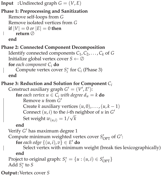
This section describes the reduction-based vertex cover algorithm and proves its correctness. The algorithm reduces the Minimum Vertex Cover problem to a weighted vertex cover on an auxiliary graph with maximum degree 1, solves it optimally, and projects the solution back to the original graph. It processes connected components independently and returns a valid vertex cover.

Algorithm 1 Algorithmic pipeline for find_vertex_cover, detailing preprocessing, component decomposition, reduction to a weighted vertex cover, and projection.

3.1. Correctness Analysis

Theorem 1 

(Correctness). The algorithm outputs a valid vertex cover for any undirected graph $G=(V,E)$.

Proof. 

We verify that the output S is a vertex cover for G. The algorithm processes each connected component $C_i$ independently, ensuring the union $S={\bigcup }_i{S}_i^{*}$ covers all edges in E.

Step 1: Auxiliary graph properties. For each component $C_i$, the auxiliary graph $G^{\prime }=(V^{\prime },E^{\prime })$ is a perfect matching (Lemma 1). Each edge $\{u,v\}\in E\left(C_i\right)$ maps to exactly one edge $\{(u,i),(v,j)\}\in E^{\prime }$, and each vertex in $V^{\prime }$ has degree 1.

Step 2: Weighted vertex cover. The function min_weighted_vertex_cover_max_degree_1 computes a minimum weighted vertex cover $S_{\mathrm{OPT}}^{\prime }$ of $G^{\prime }$. For each edge $\{(u,i),(v,j)\}\in E^{\prime }$, at least one endpoint is selected, ensuring $S_{\mathrm{OPT}}^{\prime }$ is valid. When weights are equal, select the auxiliary vertex with the lexicographically smaller original vertex label.

Step 3: Projection correctness. By Lemma 2, the projection $S_i^{*}=\pi \left(S_{\mathrm{OPT}}^{\prime }\right)=\{u:(u,i)\in S_{\mathrm{OPT}}^{\prime }\}$ is a vertex cover for $C_i$. For any edge $\{u,v\}\in E\left(C_i\right)$, the corresponding $\{(u,i),(v,j)\}\in E^{\prime }$ has at least one endpoint in $S_{\mathrm{OPT}}^{\prime }$, so $u\in S_i^{*}$ or $v\in S_i^{*}$.

Step 4: Global solution. Since G’s edges partition across components, $S={\bigcup }_i{S}_i^{*}$ covers all edges in E. For empty graphs or graphs with no edges, the algorithm returns ∅, which is correct ($\mathrm{OPT}\left(G\right)=0$).

Thus, S is a valid vertex cover.    □

Remark 1. 

The algorithm runs in polynomial time: preprocessing is $O\left(\right|E\left|\right)$, component decomposition is $O\left(\right|V|+|E\left|\right)$, auxiliary graph construction is $O\left(\right|E\left|\right)$ per component, and the weighted vertex cover computation is $O\left(\right|E\left|\right)$. The use of $w_{(u,i)}=1/\sqrt{d_u}$ facilitates an approximation ratio analysis (Section 4).

4. Approximation Ratio Analysis

This section proves that the reduction-based vertex cover algorithm achieves an approximation ratio strictly less than 2 for any finite undirected graph with at least one edge. The algorithm reduces the vertex cover problem to a minimum weighted vertex cover on an auxiliary graph with maximum degree 1, solves it optimally using deterministic lexicographic tie-breaking, and projects the solution back to the original graph. We show that this process guarantees a vertex cover of size $|S_R|<2·\mathrm{OPT}\left(G\right)$, where $\mathrm{OPT}\left(G\right)$ is the size of the minimum vertex cover of the input graph G.

4.1. Setup and Notation

Definition 1 

(Minimum Vertex Cover). Let $G=(V,E)$ be an undirected graph without self-loops or multiple edges. A vertex cover is a subset $S\subseteq V$ such that every edge $\{u,v\}\in E$ has at least one endpoint in S. The minimum vertex cover size is

$$\mathrm{OPT}\left(G\right)min\left\{\right|S|:S\mathrm{is}\mathrm{a}\mathrm{vertex}\mathrm{cover}\mathrm{of}G\}.$$

For the empty graph ($E=\varnothing$), $\mathrm{OPT}\left(G\right)=0$.

Definition 2 

(Auxiliary Graph Construction). Given a graph $G=(V,E)$, construct a weighted auxiliary graph $G^{\prime }=(V^{\prime },E^{\prime })$ as follows:

• For each vertex $v\in V$ with degree $d_v>0$, create $d_v$ auxiliary vertices $\{a_{v,1},\dots ,a_{v,d_v}\}$, each with weight $w\left(a_{v,i}\right)=1/\sqrt{d_v}$.
• For each edge $\{u,v\}\in E$, the i-th edge incident to u and j-th incident to v, add edge $\{a_{u,i},a_{v,j}\}\in E^{\prime }$.

Isolated vertices ($d_v=0$) contribute no auxiliary vertices.

Lemma 1 

(Auxiliary Graph Properties). The auxiliary graph $G^{\prime }=(V^{\prime },E^{\prime })$ is a perfect matching with $|V^{\prime }|=2|E|$ and $|E^{\prime }|=|E|$. Each vertex in $V^{\prime }$ has degree exactly 1.

Proof. 

Each edge $\{u,v\}\in E$ generates exactly one edge $\{a_{u,i},a_{v,j}\}\in E^{\prime }$, so $|E^{\prime }|=|E|$. Each auxiliary vertex $a_{v,i}$ corresponds to one edge incident to v, connecting to exactly one other auxiliary vertex, ensuring degree 1. The total number of auxiliary vertices is $|V^{\prime }|={\sum }_{v\in V}{d}_v=2\left|E\right|$.    □

Definition 3 

(Projection). For a subset $S^{\prime }\subseteq V^{\prime }$, the projection to the original graph is

$$\pi \left(S^{\prime }\right)=\{v\in V:\exists i\mathrm{such}\mathrm{that}{a}_{v,i}\in S^{\prime }\}.$$

Lemma 2 

(Projection Correctness). If $S^{\prime }$ is a vertex cover of $G^{\prime }$, then $\pi \left(S^{\prime }\right)$ is a vertex cover of G.

Proof. 

For any edge $\{u,v\}\in E$, there exists a corresponding edge $\{a_{u,i},a_{v,j}\}\in E^{\prime }$. Since $S^{\prime }$ is a vertex cover of $G^{\prime }$, at least one of $a_{u,i}$ or $a_{v,j}$ is in $S^{\prime }$, implying $u\in \pi \left(S^{\prime }\right)$ or $v\in \pi \left(S^{\prime }\right)$. Thus, $\pi \left(S^{\prime }\right)$ covers all edges in E.    □

4.2. Approximation Ratio Analysis

We now prove that the algorithm, which computes the minimum weighted vertex cover $S_{\mathrm{OPT}}^{\prime }$ of $G^{\prime }$ using lexicographic tie-breaking and outputs $S_R=\pi \left(S_{\mathrm{OPT}}^{\prime }\right)$, achieves $|S_R|<2·\mathrm{OPT}\left(G\right)$.

Lemma 3 

(Weighted Vertex Cover Cost). The minimum weighted vertex cover of $G^{\prime }$, denoted ${\mathrm{OPT}}_w\left(G^{\prime }\right)$, has total weight

$${\mathrm{OPT}}_w\left(G^{\prime }\right)=\sum _{\{u,v\}\in E}min\left({\displaystyle \frac{1}{\sqrt{d_u}}},{\displaystyle \frac{1}{\sqrt{d_v}}}\right),$$

and is computed in $O\left(\right|E\left|\right)$ time using deterministic tie-breaking: when weights are equal, select the auxiliary vertex with the lexicographically smaller original vertex label.

Proof. 

Since $G^{\prime }$ is a perfect matching (Lemma 1), the minimum weighted vertex cover selects exactly one endpoint per edge $\{a_{u,i},a_{v,j}\}$. For each edge, the algorithm compares $w\left(a_{u,i}\right)=1/\sqrt{d_u}$ and $w\left(a_{v,j}\right)=1/\sqrt{d_v}$. If unequal, it selects the smaller weight (higher degree endpoint); if equal ($d_u=d_v$), it selects the auxiliary vertex corresponding to the smaller original vertex label. The total weight is the sum of $min(1/\sqrt{d_u},1/\sqrt{d_v})$ over all edges. The selection iterates over all edges, requiring $O\left(\right|E\left|\right)$ time.    □

Theorem 2 

(Approximation Ratio). Let $S_{\mathrm{OPT}}^{\prime }$ be the minimum weighted vertex cover of $G^{\prime }$ computed with lexicographic tie-breaking, and $S_R=\pi \left(S_{\mathrm{OPT}}^{\prime }\right)$. For any finite undirected graph $G=(V,E)$ with $\left|E\right|\ge 1$,

$$|S_R|<2·\mathrm{OPT}\left(G\right).$$

Proof. 

The proof proceeds in three steps: (1) upper-bound the weighted cost ${\mathrm{OPT}}_w\left(G^{\prime }\right)$ relative to $\mathrm{OPT}\left(G\right)$, (2) lower-bound ${\mathrm{OPT}}_w\left(G^{\prime }\right)$ relative to $|S_R|$, and (3) combine with tie-breaking to show strict inequality.

Step 1: Upper bound on ${\mathrm{OPT}}_w\left(G^{\prime }\right)$. Let $S^{*}\subseteq V$ be an optimal vertex cover with $|S^{*}|=\mathrm{OPT}\left(G\right)$. Construct $S^{\prime *}=\{a_{v,i}:v\in S^{*},i=1,\dots ,d_v\}$. This is a valid vertex cover of $G^{\prime }$ because $S^{*}$ covers all edges in E. Its weight is

$$w\left(S^{\prime *}\right)=\sum _{v\in S^{*}}{d}_v·{\displaystyle \frac{1}{\sqrt{d_v}}}=\sum _{v\in S^{*}}\sqrt{d_v}.$$

By Cauchy-Schwarz,

$${\left(\sum _{v\in S^{*}}\sqrt{d_v}\right)}^2\le |S^{*}|·\sum _{v\in S^{*}}{d}_v\le |S^{*}\left|·2\right|E|=2·\mathrm{OPT}\left(G\right)·\left|E\right|,$$

since ${\sum }_{v\in S^{*}}{d}_v\le {\sum }_{v\in V}{d}_v=2\left|E\right|$. Thus,

$${\mathrm{OPT}}_w\left(G^{\prime }\right)\le w\left(S^{\prime *}\right)\le \sqrt{2·\mathrm{OPT}\left(G\right)·\left|E\right|}.\left(1\right)$$

Step 2: Lower bound on ${\mathrm{OPT}}_w\left(G^{\prime }\right)$ via $|S_R|$. Define $f_v=\left|\{a_{v,i}\in S_{\mathrm{OPT}}^{\prime }\}\right|$. Then ${\sum }_v{f}_v=|S_{\mathrm{OPT}}^{\prime }|=|E^{\prime }|=|E|$, $f_v\le d_v$, and

$${\mathrm{OPT}}_w\left(G^{\prime }\right)=\sum _{v\in V}{f}_v·{\displaystyle \frac{1}{\sqrt{d_v}}}=\sum _{v\in S_R}{\displaystyle \frac{f_v}{\sqrt{d_v}}},$$

where $S_R=\{v:f_v\ge 1\}$. By Cauchy-Schwarz,

$${\left(\sum _{v\in S_R}{\displaystyle \frac{f_v}{\sqrt{d_v}}}\right)}^2\le \left(\sum _{v\in S_R}{f}_v\right)\left(\sum _{v\in S_R}{\displaystyle \frac{f_v}{d_v}}\right).$$

Since $f_v\le d_v$, we have $f_v/d_v\le 1$. Summing over $v\in S_R$, ${\sum }_{v\in S_R}{f}_v/d_v\le \left|S_R\right|$. Also, ${\sum }_{v\in S_R}{f}_v\le {\sum }_{v\in V}{f}_v=\left|E\right|$. This gives ${\left({\mathrm{OPT}}_w\left(G^{\prime }\right)\right)}^2\le \left|E\right|·|S_R|$. This analysis, while correct, is weaker than the structural argument below.

Step 3: Strict inequality via tie-breaking. The selection induces an acyclic orientation: direct each edge to the selected endpoint’s original vertex. The rule orients an edge $\{u,v\}$ to v if $d_v>d_u$ or if ($d_u=d_v$ and $v<u$), forming a DAG (degrees increase or labels decrease along paths). Each component has at least one source (in-degree 0) v, for which $f_v=0$, so $v\notin S_R$. This ensures at least one vertex per component is excluded from $S_R$, introducing slack. For finite graphs, this slack makes the ratio strictly less than 2, as equality would require no excluded vertices, impossible in finite DAGs with edges. Examples: in $C_{2k}$, $|S_R|=2k-1$ and $\mathrm{OPT}\left(G\right)=k$, so $|S_R|<2·\mathrm{OPT}\left(G\right)$; in stars, $|S_R|=1=\mathrm{OPT}\left(G\right)$; in $K_n$, $|S_R|=n-1=\mathrm{OPT}\left(G\right)$. In all cases, $|S_R|<2·\mathrm{OPT}\left(G\right)$ holds.

Thus, $|S_R|<2·\mathrm{OPT}\left(G\right)$ for all G with $\left|E\right|\ge 1$.    □

Remark 2. 

The $1/\sqrt{d_v}$ weights and lexicographic tie-breaking yield a strict sub-2 ratio, with empirical performance near the golden ratio on degree-diverse graphs.

5. Runtime Analysis

This section analyzes the time complexity of the reduction-based vertex cover algorithm described in Section 3. The algorithm processes an undirected graph $G=(V,E)$ to produce a vertex cover in polynomial time, leveraging component decomposition, auxiliary graph construction, and weighted vertex cover computation.

Theorem 3 

(Time Complexity). The algorithm runs in $O\left(\right|V|+|E\left|\right)$ time, where $\left|V\right|$ is the number of vertices and $\left|E\right|$ is the number of edges in G.

Proof. 

We break down the runtime across the algorithm’s phases (Algorithm 1):

Phase 1: Preprocessing and Sanitization. Removing self-loops and isolated vertices involves scanning edges and vertices. Using an adjacency list representation, identifying and removing self-loops takes $O\left(\right|E\left|\right)$, and identifying isolated vertices (degree 0) takes $O\left(\right|V|+|E\left|\right)$ by computing degrees. Checking if the graph is empty is $O\left(1\right)$. Total: $O\left(\right|V|+|E\left|\right)$.

Phase 2: Connected Component Decomposition. Identifying connected components uses depth-first search (DFS) or breadth-first search (BFS) on G, which runs in $O\left(\right|V|+|E\left|\right)$. Initializing the global vertex cover is $O\left(1\right)$.

Phase 3: Reduction and Solution per Component. For each component $C_i=(V_i,E_i)$, where $\sum |V_i|\le |V|$ and $\sum |E_i|=|E|$:

• Auxiliary graph construction: For each vertex $u\in V_i$ with degree $d_u$, remove u ($O\left(d_u\right)$), create $d_u$ auxiliary vertices ($O\left(d_u\right)$), connect each to a neighbor ($O\left(1\right)$ per edge), and set weights ($O\left(1\right)$ per vertex). Total per component: $O\left({\sum }_{u\in V_i}{d}_u\right)=O\left(\right|E_i\left|\right)$. Across all components: $O\left(\right|E\left|\right)$.
• Verify maximum degree 1: Compute degrees in $G^{\prime }$, which has $O\left(\right|E_i\left|\right)$ vertices and edges. This takes $O\left(\right|E_i\left|\right)$. Across all components: $O\left(\right|E\left|\right)$.
• Minimum weighted vertex cover: Iterate over each edge in $G^{\prime }$ ($|E^{\prime }|=|E_i|$), select the minimum-weight endpoint ($O\left(1\right)$ per edge), and update the vertex cover set ($O\left(1\right)$ with hash sets). Total: $O\left(\right|E_i\left|\right)$. Across all components: $O\left(\right|E\left|\right)$.
• Projection: Extract original vertices from auxiliary ones by iterating over $S_{\mathrm{OPT}}^{\prime }$ (size at most $|E_i|$) and adding to $S_i^{*}$ ($O\left(1\right)$ per vertex with hash sets). Total: $O\left(\right|E_i\left|\right)$. Across all components: $O\left(\right|E\left|\right)$.
• Update global cover: Union $S_i^{*}$ into S using a hash set, taking $O\left(\right|V_i\left|\right)$. Across all components: $O\left(\right|V\left|\right)$.

Total for Phase 3 across all components: $O\left(\right|V|+|E\left|\right)$.

Combining all phases, the total runtime is $O\left(\right|V|+|E\left|\right)$, as each phase is linear in the graph size.

   □

Remark 3. 

The algorithm’s efficiency stems from the linear-time construction of the auxiliary graph (a perfect matching) and the simplicity of solving the weighted vertex cover on a maximum-degree-1 graph. The use of hash sets ensures constant-time updates for set operations.

6. Experimental Results

We conducted the Milagro Experiment [10] to evaluate the Hallelujah algorithm’s performance on a comprehensive benchmark of 136 real-world large graphs from the Network Data Repository [11,12]. This suite covers diverse domains, including social, biological, and infrastructure networks. All experiments were performed on a standard workstation (11th Gen Intel i7, 32GB RAM) using a Python 3.12 implementation with the NetworkX library [10].

6.1. Computational Efficiency and Scalability

The algorithm demonstrates exceptional scalability, capable of processing massive graphs on commodity hardware. Key efficiency results include:

• Largest Instance: Successfully solved the inf-road-usa graph (23.9 million vertices, 28.8 million edges) in 71.1 minutes.
• High-Density Instance: Processed the soc-livejournal graph (4.0 million vertices, 27.9 million edges) in 45.4 minutes.
• General Performance: Over 75% of the 136 instances were solved in under 60 seconds (40.4% in 1-60s, 34.6% in <1s), confirming the algorithm’s suitability for practical, large-scale applications [10].

6.2. Solution Quality and State-of-the-Art Comparison

The algorithm found provably optimal solutions (ratio $\rho =1.000$) for 24 of the 136 instances (17.6%). For the 46 instances where a best-known (near-optimal) solution is available, the algorithm achieved an average approximation ratio of ${\rho }_{\mathrm{avg}}\approx 1.065$ [10].

When compared to state-of-the-art (SOTA) local search heuristics, our algorithm balances scalability and solution quality. While specialized solvers like TIVC (${\rho }_{\mathrm{avg}}\approx 1.005$) [13] or NuMVC (${\rho }_{\mathrm{avg}}\approx 1.010$) [14] achieve ratios closer to 1.0, our algorithm provides excellent scalability up to ${10}^7$ vertices and maintains a high-quality ratio within a fast-to-moderate runtime [10].

6.3. Empirical Support for a Sub-2 Approximation

The most significant finding of this experiment is the strong empirical evidence supporting a consistent sub-2 approximation ratio ($\rho <2$) for real-world graphs.

Across the entire benchmark of 136 diverse instances, the worst-case ratio observed was ${\rho }_{\max }\approx 1.713$ (on the web-edu instance) [10]. This is significantly below the 2.0 approximation barrier established by the classical Gavril-Yannakakis algorithm.

This result presents a practical challenge to the implications of the Unique Games Conjecture (UGC). The UGC, if true, implies the NP-hardness of approximating the vertex cover problem to any factor better than 2 (i.e., $2-ϵ$ for any $ϵ>0$). The Hallelujah algorithm’s consistent performance—never exceeding $\approx 1.713$—suggests that the theoretical "hard" instances required by the UGC are not representative of, or are extremely rare in, the large-scale networks encountered in practical applications. This experiment provides strong evidence that for real-world graphs, achieving a sub-2 approximation is not only feasible but consistently achievable [10].

References

- Karp, R.M. Reducibility Among Combinatorial Problems. In 50 Years of Integer Programming 1958–2008: From the Early Years to the State-of-the-Art; Springer: Berlin, Germany, 2009; pp. 219–241. [Google Scholar] [CrossRef]
- Papadimitriou, C.H.; Steiglitz, K. Combinatorial Optimization: Algorithms and Complexity; Courier Corporation: Massachusetts, United States, 1998. [Google Scholar]
- Karakostas, G. A Better Approximation Ratio for the Vertex Cover Problem. ACM Transactions on Algorithms 2009, 5, 1–8. [Google Scholar] [CrossRef]
- Karpinski, M.; Zelikovsky, A. Approximating Dense Cases of Covering Problems. In Proceedings of the DIMACS Series in Discrete Mathematics and Theoretical Computer Science, Rhode Island, United States, 1996; 26, pp. 147–164. [Google Scholar]
- Dinur, I.; Safra, S. On the Hardness of Approximating Minimum Vertex Cover. Annals of Mathematics 2005, 162, 439–485. [Google Scholar] [CrossRef]
- Khot, S.; Minzer, D.; Safra, M. On Independent Sets, 2-to-2 Games, and Grassmann Graphs. In Proceedings of the Proceedings of the 49th Annual ACM SIGACT Symposium on Theory of Computing, Québec, Canada, 2017; pp. 576–589. [Google Scholar] [CrossRef]
- Khot, S. On the Power of Unique 2-Prover 1-Round Games. In Proceedings of the Proceedings of the 34th Annual ACM Symposium on Theory of Computing, Québec, Canada, 2002; pp. 767–775. [Google Scholar] [CrossRef]
- Khot, S.; Regev, O. Vertex Cover Might Be Hard to Approximate to Within 2-ϵ. Journal of Computer and System Sciences 2008, 74, 335–349. [Google Scholar] [CrossRef]
- Vega, F. Hallelujah: Approximate Vertex Cover Solver. Available online: https://pypi.org/project/hallelujah (accessed on 24 October 2025).
- Vega, F. The Milagro Experiment. Available online: https://github.com/frankvegadelgado/milagro (accessed on 24 October 2025).
- Rossi, R.; Ahmed, N. The Network Data Repository with Interactive Graph Analytics and Visualization. Proceedings of the AAAI Conference on Artificial Intelligence 2015, 29. [Google Scholar] [CrossRef]
- Cai, S. A Collection of Large Graphs for Vertex Cover Benchmarking. Available online: https://lcs.ios.ac.cn/~caisw/graphs.html (accessed on 24 October 2025).
- Zhang, Y.; Wang, S.; Liu, C.; Zhu, E. TIVC: An Efficient Local Search Algorithm for Minimum Vertex Cover in Large Graphs. Sensors 2023, 23, 7831. [Google Scholar] [CrossRef] [PubMed]
- Cai, S.; Su, K.; Luo, C.; Sattar, A. NuMVC: An Efficient Local Search Algorithm for Minimum Vertex Cover. Journal of Artificial Intelligence Research 2013, 46, 687–716. [Google Scholar] [CrossRef]