
Submitted:
29 October 2025
Posted:
30 October 2025
You are already at the latest version
Abstract
Pairs trading via futures calendar spreads offers a robust market-neutral approach to exploiting transient mispricings, yet real-time implementation is hindered by asynchronous trading. This paper introduces a Cointegrated Ising Spin Model for real-time signal generation in high-frequency spread trading. The model links the macro-level equilibrium of cointegration with micro-level agent interactions, representing prices as magnetizations in an agent-based system. A novel \( \Delta \)-weighted arbitrage force dynamically adjusts agents’ corrective behavior to account for information staleness. Calibrated on tick-by-tick Brent crude oil futures, the model produces a time-varying probability of spread reversion, enabling probabilistic trading decisions. Backtesting demonstrates a 74.65\% success rate, confirming the model’s ability to generate stable, data-driven arbitrage signals in asynchronous environments. The model bridges macro-level cointegration with micro-level agent interactions, representing prices as magnetizations within an agent-based Ising system. A novel feature is a \( \Delta \)-weighted arbitrage force, where the corrective pressure applied by agents in response to the standard Error Correction Term is dynamically amplified based on information staleness. The model is calibrated on historical tick data and designed to operate in real time, continuously updating its probability-based trading signals as new quotes arrive.
Keywords:
spread trading
; crude oil
; ointegrated Ising Spin Model
1. Introduction
Statistical Arbitrage and Futures Spread Trading
Trading futures calendar spreads—the simultaneous purchase and sale of futures contracts on the same asset but with different delivery months—is a cornerstone of high-frequency statistical arbitrage (SA) [10]. Such strategies aim to profit from temporary deviations in the price relationship between contracts, relying on the statistical likelihood that these mispricings will revert to a historical or theoretical equilibrium [15]. Unlike pure arbitrage, SA strategies involve risk but seek to generate market-neutral returns by exploiting these predictable patterns, which are often identified through quantitative models [15][18].
Futures contracts, due to their standardized nature and liquidity, are frequently employed in SA strategies. Inter-calendar spreads, in particular, are a popular strategy involving the simultaneous purchase of a futures contract for one delivery month and the sale of another futures contract for a different delivery month, on the same underlying asset [10]. These spreads can reflect market expectations about future supply and demand, storage costs (cost of carry), and convenience yields. Deviations in these spreads from their historical norms or fundamentally expected levels can present SA opportunities, assuming mean reversion or predictable patterns in the term structure. Spread trading strategies, particularly those based on pairs of liquid instruments, are widely employed across financial markets. These strategies rely on identifying temporary deviations in price relationships—often modeled via cointegration—that are expected to mean-revert over time. Pairs may consist of contracts on the same underlying asset with different maturities (calendar spreads), or different but closely related assets (inter-market spreads), such as futures, ETFs, or equities with fundamental or statistical linkages. The effectiveness of such strategies depends critically on the availability of high-frequency trading data, adequate market depth, and minimal execution delays.
Although the framework developed in this paper is general and applicable to any such pair exhibiting liquid and asynchronous trading, we illustrate its implementation using the Brent crude oil futures of the first and second-month. These contracts are among the most actively traded globally, offering a natural testbed for evaluating high-frequency arbitrage strategies under real-world conditions.
2. Literature Review
The model presented in this paper draws upon several distinct but interconnected streams of financial and econophysics literature: statistical arbitrage focusing on pairs trading and cointegration, agent-based modeling using Ising spin systems, and the analysis of high-frequency market dynamics.
2.1. Statistical Arbitrage, Pairs Trading, and Cointegrated Models
A foundational concept in quantitative finance is the exploitation of temporary deviations from statistically identified equilibrium relationships between assets, a field formally known as Statistical Arbitrage (SA) [15]. The primary goal of SA is to construct market-neutral portfolios that profit from the expected correction of these mispricings, thereby isolating alpha from broader market movements. The most prominent implementation of this concept is pairs trading, a strategy involving a long position in an underpriced asset paired with a short position in a related, overpriced asset [9][10][18]. The success of this approach hinges on identifying assets whose prices exhibit a stable long-run relationship.
The theoretical underpinnings for identifying such relationships often stem from concepts like Arbitrage Pricing Theory (APT). APT suggests that if two securities share identical risk factor exposures, their expected returns over a given period should be the same [18]. Deviations from this parity, manifested in the spread between their (log) prices, are expected to be temporary and mean-reverting, forming the basis for pairs trading.
The econometric cornerstone for identifying mean-reverting spreads between non-stationary price series is the concept of cointegration, famously developed by Engle and Granger [7]. If two non-stationary time series, say the log-prices and , are cointegrated, there exists a linear combination
(the spread, or cointegrating residual) that is stationary. The parameter is the cointegration coefficient, and (or an intercept in the cointegrating relation) represents the long-run equilibrium level of the spread.
The dynamics of cointegrated systems are often captured by a Vector Error Correction Model (VECM). A VECM describes how the individual series adjust when the spread deviates from its long-run equilibrium. A common representation of the VECM, including first-order lagged difference terms for short-run dynamics, is:
where and are the speeds of adjustment, is the error correction term (ECT) from the previous period, and are coefficients for the first-order lagged differences of and [8,18]. More general VECM representations would include higher-order lags of these differences.
For the VECM system to be stable and mean-reverting, the adjustment speeds and must possess specific signs. With the ECT defined as , stability requires and (for ) . These signs ensure that a positive deviation (ECT ) is corrected by a decrease in and/or an increase in , and vice versa for a negative deviation. The model presented here adapts this error-correction principle, translating the statistical adjustment speeds into a ’PullTerm’ that directly influences agent behavior at the micro-level, as detailed in Section 3.
Trading strategies are then built by taking positions when the spread deviates significantly (e.g., by a threshold ) from its mean , expecting a reversion [9,18]. The Stock-Watson common trends model provides another perspective, suggesting that cointegrated series share common underlying non-stationary components that are nullified in the cointegrating relationship [17,18]. Advanced pairs trading frameworks may also incorporate tools like Kalman filters for dynamic hedge ratio estimation and other indicators like the Hurst exponent to assess mean-reversion persistence [10].
However, a critical limitation of the classic VECM framework (Eqs. 2 and ) is the assumption that error correction is driven solely by the disequilibrium of the immediately preceding period. In high-frequency markets, this assumption is often violated, as information lags and gradual price discovery can lead to delayed adjustments [10]. This issue of "delayed cointegration" has recently been explored from a continuous-time, mathematical finance perspective. For instance, Yan et al. [19] model the cointegrated price process as a path-dependent stochastic delay differential equation (SDDE), representing the limit of a high-order VECM. Their work focuses on deriving a mathematically optimal portfolio allocation by solving a system of Riccati partial differential equations.
While such analytical approaches provide a rigorous theoretical foundation for delayed adjustment, they are often difficult to implement and calibrate directly with discrete, asynchronous tick data. The present study addresses the same fundamental problem of delayed error correction but from a complementary, micro-founded perspective. Instead of modeling the continuous price path,this study uses an agent-based framework to model the discrete event-time dynamics. The model’s key innovation—a -weighted arbitrage force—explicitly incorporates the empirically observed time staleness of trades, offering a practical, data-driven mechanism to account for delayed information processing in a high-frequency environment.
2.2. Ising Models in Finance
The Ising model, originating from statistical mechanics to describe ferromagnetism, has found extensive application in finance and econophysics as a framework for modeling agent-based interactions and collective phenomena [6,14]. The application of ferromagnet theory to social imitation, where individual agent decisions (spins) are influenced by neighbors and global fields, provides a theoretical basis for these models [4]. In this context, agents (traders) are represented by spins, typically binary (), indicating buy/sell decisions or bullish/bearish sentiment. The aggregate state of the system is often measured by the total magnetization , representing the overall market mood or trend [2,6]. Callen and Shapero [4] discuss how concepts like order parameters (e.g., alignment of fish, phase angle of fireflies) and even a "social temperature" can be analogous to physical systems, further justifying the use of such physics-inspired models for collective human behavior.
Agent decisions (spin flips) in financial Ising models are governed by a local field . Bornholdt’s influential work [2], for example, models this local field to include:
- Global Field/External Influence (): An external field, often related to the general state of the market (e.g. magnetization ), can influence individual spins. In many financial Ising models, such as Bornholdt’s, this term often induces an anti-ferromagnetic tendency (minority game characteristic), where agents are incentivized to take positions contrary to the majority if they believe profits lie in being contrarian [2,6]. This component is crucial for generating complex dynamics such as "expectation bubbles" and intermittency. Note: this is distinct from the ECM adjustment speeds .
- Stochasticity/Temperature (): The probability of a spin flip is often a logistic function of the local field, , where (inverse temperature) controls the randomness of agent decisions. High (low temperature) implies more deterministic behavior based on the local field [6]. This can be seen as analogous to the concept of "social temperature", where higher randomness equals higher social temperature [4].
Ising models, particularly configurations like those proposed by Bornholdt [2] and further explored by others (e.g., Kaizoji et al. [12], Dvořák [6]), have been successful in replicating several stylized facts of financial markets. These include volatility clustering, heavy tails in return distributions, and the slow decay of autocorrelation in absolute returns [5,6,14]. Kukacka and Kristoufek [14] found that the Bornholdt (2001) model exhibited a strong tendency towards multifractal behavior, a complex dynamic feature observed in real financial data, arising from its inherent correlation structure. The "frustration" mechanism in such models, stemming from competing influences (e.g., herding vs. contrarian global field), is key to generating rich market dynamics.
3. A Probabilistic Agent-Based Model of Spread Reversion
The analytical framework presented herein bridges the gap between purely statistical time series models (like VECM for cointegration) and the micro-foundations of simulation-based Agent-Based Models. It proposes a hybrid framework where the perceived market disequilibrium—derived from a macro-level cointegrating relationship—directly influences micro-level agent decisions, creating a novel feedback loop for modeling asynchronously traded, cointegrated assets. Conventional econometric models, such as VECM, are inherently retrospective and assume synchronous price discovery. In contrast, the model proposed here is designed for live implementation, continuously ingesting market quotes to generate real-time spread-trading signals
3.1. Theoretical Foundation and Empirical Implementation
The formal specification of this framework requires distinguishing between the true underlying market sentiment and what is observable at any given moment, explicitly accounting for the asynchronicity of trades. In the theoretical model, for each contract , a latent magnetization represents the true, unobserved aggregate sentiment of all agents. The observed magnetization, , only updates when a trade occurs, with the time elapsed since the last trade denoted by .
A core challenge in high-frequency markets is that asset prices do not update simultaneously. To conceptualize how agents might internalize this, we can define a theoretical, staleness-adjusted Error Correction Term (ECT′), where the perceived spread is adjusted based on the age (staleness) of the last trade in each contract. This adjusted ECT′ reflects a hypothetical perception of disequilibrium that discounts stale price observations. Conceptually, this could be calculated using the last observed market sentiment (magnetization) for each contract, weighted by its staleness:
where is an exponential weighting function modeling the decay of information relevance. While this ECT′ provides the theoretical motivation, this study’s practical implementation models this effect more directly by applying a -weighting to the arbitrage force that agents exert in response to the standard, empirically observed ECT, as detailed in Section 3.3.
To operationalize this framework for empirical application, we ground the model in the results of the preliminary VECM analysis. The observable spread at any time t, denoted , is defined as the cointegrating residual, or the empirical Error Correction Term (ECT), from the estimated long-run relationship:
where and are the parameters for the cointegrating vector and the long-run mean, respectively, estimated from the VECM. **This empirically observed disequilibrium, , serves as a direct and tractable proxy for the theoretical disequilibrium otherwise captured by the difference in latent magnetizations.** The model’s core function is to compute the conditional probability that this spread will revert towards its mean. This is achieved by simulating the collective behavior of a heterogeneous agent population partitioned into two distinct behavioral archetypes: trend-followers and contrarians.
3.2. The Agent-Based Ising Spin Model
The evolution of the latent magnetization is driven by the collective decisions of individual agents, modeled as spin flips. The probability of an agent i adopting a positive spin (e.g., a bullish stance) for contract X at time t is governed by a logistic function of a "local field," :
The local field synthesizes the forces influencing an agent’s decision at time t, based on information available at :
The first two terms represent standard forces in financial Ising models: herding/imitation and a contrarian reaction to the market trend. The third term, the `PullTerm`, is the novel component that directly links the agent’s decision to the cointegrating relationship. It quantifies the arbitrage pressure derived from the perceived disequilibrium, as defined in the empirical implementation by Equations (10) and ().
3.3. Microfoundations of Agent Behavior and Local Field Specification
The model’s dynamics are driven by the aggregate decisions of this heterogeneous agent population. Let and represent the time elapsed (staleness) since the last trade for contracts A and B, respectively. The decision calculus for each agent type is informed by a synthesis of momentum and mean-reversion signals.
3.3.1. Modeling Agent Influences
The forces acting upon the agents are designed to capture well-documented financial phenomena: herding, momentum-chasing, and arbitrage-driven error correction.
First, a Herding/Momentum Influence () captures the tendency for social imitation, where agents’ decisions are influenced by the perceived aggregate sentiment of the market. This is formalized by the simulated market sentiment from the previous period:
This term creates a feedback loop where a tendency to buy (or sell) in one period increases the probability of similar behavior in the next.
Second, a pure Follower Influence () represents the behavior of chartists or momentum traders who act on recent price changes. This force is responsible for amplifying spread deviations. Its strength is governed by the parameter :
A positive and significant ensures the model can generate the positive feedback dynamics that temporarily drive prices away from equilibrium.
Third, the Contrarian Influence (The `PullTerm`) is the critical error-correction force that underpins the mean-reverting tendency of the spread. It represents the behavior of arbitrageurs who identify deviations from the long-run equilibrium and trade to correct them. This term is the practical implementation of the staleness-weighted arbitrage response motivated by the theoretical ECT’ concept. It is a function of the spread’s deviation from its mean, scaled by the adjustment speed parameter, . Critically, it incorporates information staleness, where the parameter models the degree to which arbitrageurs amplify their reaction based on the age of price data:
The negative sign ensures that a positive spread deviation () generates a negative (sell) pressure. The term means that the corrective force is amplified by staleness.
3.3.2. Agent Decision Probabilities
These distinct informational influences are synthesized into a "local field", , for each agent type, representing the net decision-making force.
The translation of this deterministic field into a stochastic decision is governed by a logistic function. The parameter , analogous to the inverse temperature in statistical mechanics, controls the rationality or noise level of the agents.
The average buy probability for the contrarian agent group is the arithmetic mean: .
3.3.3. Market-Level Aggregation and Reversal Probability
The micro-level decisions are aggregated to yield a market-level signal, reflecting the market ecology. The parameter represents the proportion of contrarian agents in the total population, .
Finally, this aggregate probability is translated into the model’s ultimate prescriptive output: the conditional probability of mean reversion, . If the spread is too high (), reversion implies selling.
3.4. Parameter Estimation via Trading Simulation
The estimation of parameters for the proposed agent-based model presents a formidable challenge. The high-dimensional latent state space, representing the configuration of all agent spins, renders conventional methods such as Maximum Likelihood Estimation (MLE) computationally infeasible due to an intractable likelihood function. Similarly, while the Simulated Method of Moments (SMM) is a viable alternative for many Agent-Based Models, it focuses on matching a set of pre-selected statistical properties (moments) of the empirical data. Given that the primary goal of this research is to develop a framework for a profitable trading strategy, we adopt a more direct and performance-oriented estimation approach: "simulation-based optimization". Instead of matching statistical moments, this methodology defines an objective function based on the success rate of a trading strategy derived from the model itself. The model parameters are then optimized to maximize this performance metric over the historical dataset, directly aligning the parameter estimation process with the model’s ultimate application. The model’s free parameters, encapsulated in the vector , are optimized by maximizing the historical performance of a trading strategy.
3.4.1. Trading Signal Generation
A trade signal is generated when the model’s probabilistic output exceeds a calibrated threshold, indicating a high likelihood of mean reversion.
- Sell Signal Generation: A signal to sell the spread is generated at time t if and the reversal probability exceeds a sell threshold ().
- Buy Signal Generation: A signal to buy the spread is generated at time t if and the reversal probability exceeds a buy threshold ().
For the backtest, the trading strategy’s logic is defined by a sophisticated, dual-filter trigger mechanism that requires a specific alignment of statistical conviction with confirming market dynamics. A trade signal is generated only when a set of stringent conditions are met: for a sell signal, for example, the spread must be overvalued (), the model must indicate a high probability of reversion (), and recent positive momentum in the spread must validate the entry point. Buy signals are generated symmetrically. This dual requirement acts as a powerful safety mechanism, ensuring the strategy enters a trade precisely as a strong deviation shows signs of exhaustion, rather than attempting to trade against adverse momentum.
3.4.2. Defining a Successful Trade
A trade executed at time t is assessed for success based on the price movement in the subsequent tick, . A trade is deemed successful if the spread moves in the predicted direction.
- A sell trade is successful if the spread decreases at (i.e., ).
- A buy trade is successful if the spread increases at (i.e., ).
3.4.3. Hybrid Objective Function for Optimization
Optimizing for the raw success rate is a direct approach, but it ignores the probabilistic confidence of each signal. A more robust methodology evaluates the model’s probabilistic accuracy, but only for those instances that trigger a trade. This ensures the optimization focuses on improving actionable forecasts. To balance signal quality with overall trading performance, we define a hybrid objective function.
First, we define the realized outcome of a trade signal issued at time t. Let be a binary variable indicating if the spread reverted in the subsequent period, :
Next, we define the set of time steps where a trade signal is generated, denoted :
The objective is to maximize the statistical consistency between the forecast and the outcome for all . This is captured by a conditional Mean Squared Error (MSE) objective:
where is the number of trade signals. If no trades are generated, the objective is 0.
To reconcile signal quality with trading frequency, this calibration metric is combined with the raw trading success rate, , forming the final hybrid objective function:
where is a weighting parameter. This objective function is maximized over the training dataset using a global optimization algorithm.
4. Empirical Implementation and Calibration of the Cointegrated Ising Spin Model
The empirical validity and operational viability of the Cointegrated Ising Spin Model (CISM) are established through its implementation and calibration as a novel framework for generating real-time, probabilistic trading signals in high-frequency environments. The Cointegrated Ising Spin Model establishes a sophisticated synthesis between macro-level econometric principles and micro-level agent dynamics by conceptualizing the prices of two cointegrated futures contracts as aggregate magnetizations emerging from an underlying Ising spin system. Within this system, agent decisions are governed by a triad of forces—herding, momentum, and arbitrage—the last of which incorporates a central methodological advance: a novel -weighted adjustment mechanism. This mechanism dynamically corrects for the informational staleness inherent in asynchronous trade arrivals, a feature of paramount importance for live operational viability. The empirical exercise presented herein is therefore not a conventional backtest but rather the crucial training and calibration phase for a real-time decision engine. Its dual objectives are, first, to demonstrate the model’s capacity to be robustly trained on high-frequency, event-time tick data, and second, to verify that the estimated parameters yield economically meaningful and stable dynamics requisite for reliable deployment in live trading conditions.
The empirical validation is conducted using high-frequency tick data for the two most liquid Brent crude oil futures contracts—the front-month (LCOc1) and second-month (LCOc2)—sourced from the LSEG Eikon platform and traded on the Intercontinental Exchange (ICE) in London. Each contract represents 1,000 barrels of crude oil, is quoted in U.S. dollars per barrel with a minimum tick size of $0.01, and adheres to a standard expiration schedule central to calendar-spread trading. The ICE Brent futures market operates electronically on a near-continuous basis (02:00 to 23:00 London time) and exhibits a well-defined intraday liquidity profile that peaks during the London–New York session overlap, rendering it an ideal environment for this study. For the calibration phase, the training dataset comprises a representative trading day, 20 June 2025, from 09:30 to 23:00 London time. A raw tick-by-tick capture at a one-second sampling rate initially yielded approximately 42,000 time-stamped observations. To construct an event-time series reflective of actual market activity, non-trading intervals were systematically removed, retaining only timestamps with at least one trade in either contract. This filtering process resulted in a final dataset of approximately 16,000 observations, corresponding to an average trade arrival in the spread every 2.6 seconds. This resultant asynchronicity is not treated as a data imperfection but is instead embraced as a fundamental market characteristic that the CISM is architected to exploit. The elapsed time between consecutive trades, denoted , becomes a direct and essential input that modulates the model’s arbitrage intensity. When operationalized, the same measure is computed continuously from the incoming market data feed, allowing the model to dynamically adjust its internal state and generate updated trading probabilities at the native frequency of the market itself. To our knowledge, this work represents the first empirical realization of an Ising-based model specifically designed for, and validated on, asynchronous financial time series. Before proceeding to the calibration of the Cointegrated Ising Spin Model, it is essential to formally establish the statistical properties of the underlying price series and confirm the existence of a long-run equilibrium relationship, which is a fundamental prerequisite for the model. The initial step in this preliminary analysis is to examine the descriptive statistics of the processed, event-time data series, which are presented in Table 1.
A Vector Error Correction Model (VECM) is estimated to confirm the presence of a long-run equilibrium. The spread, or cointegrating residual, is defined as:
where is the cointegrating coefficient and is the long-run equilibrium level. The VECM specification is given by:
where and represent the speeds of adjustment towards equilibrium, and , capture short-run dynamic effects.
The VECM estimation results, presented in Table 2, provide strong statistical evidence for a stable cointegrating relationship. The estimated cointegrating coefficient is highly significant and economically intuitive, reflecting a market in weak contango where the forward price trades at a slight premium to the spot price, consistent with storage and financing costs between contract expiries.
The adjustment speed parameters are both statistically significant and possess the correct signs for a stable system. The negative sign of indicates that the front-month contract decreases in price to correct a positive disequilibrium, while the positive sign of shows the second-month contract increases. The relative magnitudes suggest an asymmetric adjustment process where the more liquid front-month contract bears approximately 56% of the total correction. The significant short-run coefficients and reveal strong positive feedback and momentum spillover between contracts, characteristic of cointegrated futures trading in high-frequency environments.
Figure 1 visually confirms the stationarity and mean-reverting behavior of the Error Correction Term, providing the statistical foundation upon which the real-time trading strategy is built.
4.1. Agent-Based Model Calibration and Trading Performance
Following the establishment of cointegration, this study calibrates the agent-based model using a performance-driven methodology specifically designed for real-time operation. The model’s key innovation is a -weighted arbitrage force that dynamically amplifies corrective pressure based on information staleness, making it uniquely suited for asynchronous high-frequency environments where trade arrivals are irregular.
Model parameters are optimized using a hybrid objective function that balances probabilistic forecast accuracy with raw trading success:
where measures the conditional mean squared error between predicted and realized reversals on trade events, and is the raw in-sample success rate. Optimization employs a staged approach combining coarse grid search, simulated annealing, and derivative-free local solvers.
The calibrated parameters, presented in Table 3, reveal a compelling market ecology dominated by sophisticated arbitrage activity. The high proportion of contrarian agents () suggests an environment rich with latent arbitrage capital poised to enforce mean reversion. The nearly equal magnitudes of momentum strength () and contrarian strength () describe a high-tension equilibrium where momentum-driven deviations meet aggressive corrective responses.
The high agent determinism () indicates rational, purposeful response to market signals. Crucially, the substantial staleness weight () confirms the importance of the -weighted arbitrage mechanism, revealing that information staleness amplifies rather than degrades perceived arbitrage opportunities in this market.
The model’s practical performance is evaluated through comprehensive backtesting. Table 4 details the trading results, demonstrating the effectiveness of using the model’s probabilistic output for real-time signal generation.
The backtest yielded 217 trades with an overall success rate of 74.65%. The strategy demonstrates nuanced state-dependent behavior: stricter sell conditions generated fewer trades (80) but higher success (78.75%), while slightly more lenient buy thresholds permitted more entries (137 trades) to capture violent snap-back reversals while maintaining strong performance (72.26%). This asymmetry likely reflects day-specific microstructural effects that the model successfully navigates.
4.2. Model Diagnostics and Dynamics
An examination of the key statistical series provides crucial insight into the model’s inner workings and validates the trading strategy’s premises. Table 5 presents distributional properties of both the Error Correction Term and the model’s primary output, the conditional probability of reversion ().
The ECT’s stationarity is confirmed by a runs test that decisively rejects the random walk null hypothesis (Z-Score = -45.72, p < 0.01), establishing that spread deviations are indeed temporary. The distribution of is well-behaved and centered (mean 0.3943, median 0.3682), indicating the model is discerning and does not perpetually signal high reversion likelihood. The negative excess kurtosis (-1.326) suggests a platykurtic distribution capable of generating a wide range of probability values.
The model’s effectiveness emerges most clearly in the distribution tails. A powerful relationship exists where large, infrequent spread deviations trigger sharp increases in reversion probability. When the ECT reaches its 95th percentile (deviation of +0.0874), the reversal probability jumps to 0.8645—far exceeding trading thresholds. This relationship strengthens further at the 99th percentile. This dynamic is precisely what the trading strategy exploits: lying in wait for high-conviction forecasts that occur only during significant market dislocations (top 5-10% of spread deviations).
4.3. Robustness and Sensitivity Analysis
This study conducts targeted sensitivity analyses to validate the model’s architecture against overfitting and establish parameter necessity.
- Staleness Weight (): Reducing the calibrated value () by an order of magnitude materially decreased both trade signals and success rate, providing strong evidence that the -weighted arbitrage force is a primary source of predictive edge.
- Agent Determinism (): Systematically lowering compressed the predictive distribution of toward 0.5, eroding signal clarity and reducing performance. This validates that strategy success depends on identifying high-conviction moments requiring agent rationality.
- Relative Balance of Forces (): Altering the near-equal ratio of momentum to contrarian strength induced regime shifts. Higher ratios created trend-dominated markets with lower success rates; lower ratios led to passive markets with insufficient trades. This demonstrates critical sensitivity to the precise competitive balance between opposing market forces.
These analyses collectively demonstrate that the model’s performance arises not from any single parameter but from the synergistic interplay of its core features: staleness amplification, agent determinism, and the delicate balance between trend and counter-trend forces. The architecture proves robust to perturbations, with performance degradation following predictable patterns when key mechanisms are compromised.
5. Discussion
The empirical results demonstrate the potential of the proposed Cointegrated Ising Spin framework. Before concluding, it is useful to contextualize the model’s contribution by comparing its core features to those of traditional financial and econophysical models, and to discuss the study’s limitations and avenues for future research.
5.1. Model Novelty and Strategic Value
While the proposed framework builds upon concepts from econophysics, it introduces key innovations that tailor it specifically to high-frequency statistical arbitrage, offering distinct advantages over traditional approaches. This model is designed as a real-time signal generator for non-directional arbitrage strategies. Its core logic is not limited to futures calendar spreads but can be applied to any pair of cointegrated assets–such as cross-listed equities, related ETFs, or inter-commodity spreads–that exhibit strong mean-reverting forces and are traded asynchronously at high frequencies.
The model’s novelty can be summarized in three key departures from the standard approaches in both econometrics and agent-based modeling:
- Endogenous, Econometrically-Grounded Arbitrage Force: Traditional agent-based and Ising models (e.g., [2,12]) often rely on abstract or exogenous fundamental values, deriving agent decisions from forces like local herding and a global contrarian field. In contrast, the model’s primary driver is the novel `PullTerm’. This term is an endogenous force derived directly from an empirically estimated, macro-level econometric relationship–the cointegration vector. This elegantly anchors micro-level agent behavior to an observable, mean-reverting macro-level equilibrium, bridging the gap between econometrics and econophysics and providing a theoretically sound foundation for the trading signals.
- Explicit Modeling and Exploitation of Asynchronous Time: Standard time-series models and Ising models struggle with asynchronous data, often assuming synchronous time steps (). The model’s key innovation is how it operationalizes a -weighted arbitrage force. By explicitly incorporating the real-world time elapsed since the last trade () for each asset, this framework turns asynchronicity from a data problem into a source of alpha. This dynamic weighting of the corrective force yields a more accurate, real-time response to market disequilibrium that is uniquely suited for generating signals from tick-level data.
- A Prescriptive, Probabilistic Output: The output of many quantitative models is a latent state (e.g., aggregate magnetization) or a binary signal. The model’s primary output is a prescriptive, conditional probability of mean reversion. By aggregating agent decisions, the model directly calculates an instantaneous, actionable probability that the spread will converge. This transforms the model from a purely descriptive tool into a sophisticated, probabilistic signal generator, allowing for the construction of more nuanced, risk-aware strategies that move beyond static threshold rules.
5.2. Limitations and Future Research
Despite the promising results, it is crucial to acknowledge the limitations of this study, which provide clear avenues for future work.
First, the model parameters were calibrated and backtested on a historical dataset from a single trading day. This approach, while useful for demonstrating the framework’s internal consistency and potential, carries a significant risk of overfitting. A crucial next step is to perform rigorous out-of-sample validation by training the model on data from one period and testing its performance on subsequent, unseen data to assess its true predictive power and robustness across different market regimes.
Second, the backtest was conducted without explicit transaction costs. In a live market, the bid-ask spread, commissions, and potential slippage represent direct and unavoidable costs that would reduce the reported profitability. A comprehensive assessment requires incorporating these frictions, though the highly liquid nature of the Brent futures market provides a robust foundation for the model’s initial validation.
Third, the small trade sample (217 trades) generated in the one-day backtest is a limitation for conclusively validating a high-frequency strategy. A longer testing period generating a larger number of trades is required to confirm the statistical significance and robustness of the performance.
Finally, the framework itself has scope for improvement. Parameter calibration could be enhanced with more dynamic optimization methods to better adapt to changing market conditions. The objective function could also be modified to maximize risk-adjusted metrics like the Sharpe ratio instead of raw success rates. Further extensions could involve endogenizing the trade arrival process or incorporating a wider variety of heterogeneous agent types with different memory lengths and risk tolerances.
6. Conclusions
This study demonstrates that combining econometric cointegration with agent-based modeling can yield a powerful, probabilistic trading framework for asynchronous markets. The Cointegrated Ising Spin Model integrates the statistical structure of the VECM with the behavioral microdynamics of agents, translating macro-level error correction into real-time, probability-based trading signals. Applied to Brent crude oil futures, the model achieved a 74.65% predictive success rate, validating the economic relevance of the -weighted arbitrage mechanism.
This paper has addressed the significant challenge of modeling and trading cointegrated, asynchronously traded assets, with a direct application to Brent crude oil futures spreads. We proposed a novel hybrid framework that integrates the macro-level dynamics of a Vector Error Correction Model (VECM) with the micro-foundations of an agent-based Ising spin model. The key innovation is the introduction of a `PullTerm` into the agent decision-making process, ...which is driven by a -weighted arbitrage force that explicitly accounts for information staleness.
The parameters of the agent-based model were estimated through a direct, performance-driven optimization of a probability-based trading strategy, aligning the model’s calibration with its practical goal. The in-sample backtest of the optimized strategy yielded a strong overall success rate of 74.65%, highlighting the potential of using such hybrid agent-based models to move beyond static-threshold arbitrage strategies toward more dynamic, probability-driven approaches.
By calibrating the Cointegrated Ising Spin Model on historical tick data and subsequently feeding it with live market quotes, the proposed framework establishes a deployable architecture for automated spread trading. This dual design—training offline and executing online—extends the conventional boundaries of statistical arbitrage by transforming an econometric model into an adaptive, continuously operating decision system. In doing so, it enables real-time monitoring and signal generation in markets where asynchronicity and information staleness are inherent features of price formation.
Overall, this study demonstrates that bridging statistical time-series modeling with agent-based simulation yields a robust and versatile framework for capturing the microdynamics of spread reversion. The methodology provides a practical blueprint for next-generation, non-directional arbitrage strategies capable of functioning in live trading environments. Its flexibility allows seamless adaptation across asset classes characterized by liquidity, asynchronous price discovery, and mean-reverting behavior, paving the way for a new class of real-time, probabilistic trading systems grounded in sound econometric principles.
Acknowledgments
The author would like to thank David H Bolton for programming support.
References
- Alfarano, S., Lux, T., Wagner, F. (2005). Estimation of agent-based models: the case of an asymmetric herding models. Computational Economics, 26, 19–49.
- Bornholdt, S. (2001). Expectation Bubbles in a Spin Model of Markets: Intermittency from Frustration across Scales. International Journal of Modern Physics C, 12(05), 667–674.
- Brock, W. A. & Hommes, C. H. (1998). Heterogeneous Beliefs and Routes to Chaos in a Simple Asset Pricing Model. Journal of Economic Dynamics and Control, 22(8-9), 1235–1274.
- Callen, E., & Shapero, D. (1974). A theory of social imitation. Physics Today, 27(7), 23–28.
- Cont, R. (2001). Empirical Properties of Asset Returns: Stylized Facts and Statistical Issues. Quantitative Finance, 1(2), 223–236.
- Dvořák, P. (2012). From Microscopic Rules to Macroscopic Phenomena: Ising Model in Finance. (Unpublished bachelor thesis). Charles University in Prague.
- Engle, Robert F. and C. W. Granger. (1987). Co-integration and Error Correction: Representation, Estimation and Testing. Econometrica, 55(2), 251–276.
- Enders, Walter. (1995). Applied Econometric Time Series. New York: John Wiley & Sons, Inc.
- Gatev, Evan, G., William, N. Goetzmann, and K. Greet Rouwenhorst. (1999). Pairs Trading: Performance of a Relative Value Arbitrage Rule. NBER Working Papers 7032, National Bureau of Economic Research Inc.
- He, C., Wang, T., Liu, X., & Huang, K. (2023). An innovative high-frequency statistical arbitrage in Chinese futures market. Journal of Innovation & Knowledge, 8(2023), 100429.
- Hommes, C. H. (2006). Heterogeneous Agent Models in Economics and Finance. In L. Tesfatsion & K. L. Judd (editors), Handbook of Computational Economics, volume 2, chapter 23, pp. 1109–1186. Elsevier.
- Kaizoji, T., S. Bornholdt, & Y. Fujiwara (2002). Dynamics of Price and Trading Volume in a Spin Model of Stock Markets with Heterogeneous Agents. Physica A: Statistical Mechanics and its Applications, 316(1-4), 441–452.
- Kirman, A. (1993). Ants, rationality, and recruitment. The Quarterly Journal of Economics, 108(1), 137–156.
- Kukacka, J., & Kristoufek, L. (2020). Do ‘complex’ financial models really lead to complex dynamics? Agent-based models and multifractality. Journal of Economic Dynamics and Control, 113, 103855.
- Lazzarino, M., Berrill, J. and Šević, A. (2018). What Is Statistical Arbitrage? Theoretical Economics Letters, 8, 888-908.
- Sieczka, P. & J. A. Holyst (2007). A Threshold Model of Financial Markets. arXiv:0711.3106 [q-fin.ST].
- Stock, James H. and Mark W. Watson. (1988). Testing for Common Trends. Journal of the American Statistical Association, 83(404), 1097–1107.
- Vidyamurthy, G. (2004). Pairs Trading: Quantitative Methods and Analysis. John Wiley & Sons.
- Yan, T., Chiu, M. C., & Wong, H. Y. (2022). Pairs trading under delayed cointegration. Quantitative Finance, 22(9), 1627–1648.
Figure 1.
Time Series of the Estimated Error Correction Term (ECT). The series represents the deviation from the long-run equilibrium, calculated as . The plot visually confirms the stationary, mean-reverting nature of the spread.
Figure 1.
Time Series of the Estimated Error Correction Term (ECT). The series represents the deviation from the long-run equilibrium, calculated as . The plot visually confirms the stationary, mean-reverting nature of the spread.
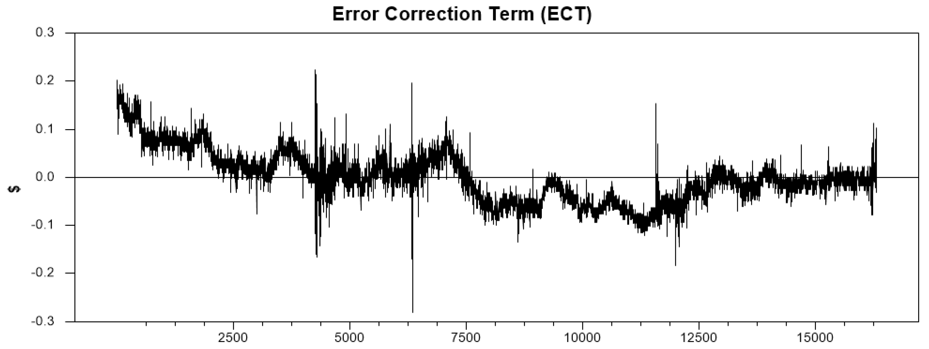

Table 1.
Summary Statistics for Futures Prices.
| Series | Observations | Mean ($) | Std. Dev. | Minimum ($) | Maximum ($) |
|---|---|---|---|---|---|
| (LCOc1) | 16,318 | 76.78 | 0.359 | 75.61 | 77.50 |
| (LCOc2) | 16,318 | 75.24 | 0.327 | 74.09 | 75.86 |
Table 2.
VECM Estimated Coefficients.
| Variable | Coefficient | Std. Error | T-Statistic | p-value |
|---|---|---|---|---|
| Adjustment Speeds | ||||
| -0.02574 | 0.00214 | -12.01 | 0.0000 | |
| 0.02011 | 0.00225 | 8.93 | 0.0000 | |
| Cointegrating Parameter | ||||
| 1.02045 | 0.00005 | 20596.37 | 0.0000 | |
| Short-Run Dynamics | ||||
| 0.41446 | 0.00257 | 161.15 | 0.0000 | |
| 0.33730 | 0.00210 | 160.28 | 0.0000 | |
Table 3.
Calibrated Parameters for the Agent-Based Model.
| Parameter | Calibrated Value |
|---|---|
| Proportion of Contrarians, | 78 |
| Agent Determinism, | 5.387 |
| Momentum Strength, | 34.225 |
| Contrarian Strength, | 34.888 |
| Staleness Weight, | 25.282 |
| Sell Threshold, | 0.504 |
| Buy Threshold, | 0.454 |
Table 4.
Trading Strategy Performance.
| Trade Execution Summary | Performance Summary | ||
|---|---|---|---|
| Sell Trades | 80 | Overall Success Rate | 74.65% |
| Successful Sells | 63 | Sell Success Rate | 78.75% |
| Buy Trades | 137 | Buy Success Rate | 72.26% |
| Successful Buys | 99 | Total Trades | 217 |
Table 5.
Descriptive Statistics: ECT and Reversal Probability.
| Metric | ECT (Spread) | Prob(Reversal) |
|---|---|---|
| Summary Statistics | ||
| Mean | 0.0002 | 0.3943 |
| Std. Dev. | 0.0525 | 0.2905 |
| Skewness | 0.5127 | 0.2411 |
| Kurtosis (excess) | 0.3251 | -1.3260 |
| Minimum | -0.2815 | 0.0000 |
| Maximum | 0.2238 | 0.9489 |
| Percentiles | ||
| 1st | -0.0946 | 0.0003 |
| 5th | -0.0767 | 0.0109 |
| 25th | -0.0377 | 0.1170 |
| 50th (Median) | -0.0036 | 0.3682 |
| 75th | 0.0293 | 0.6823 |
| 95th | 0.0874 | 0.8645 |
| 99th | 0.1510 | 0.8934 |
| Stationarity Test | ||
| Runs Test (Z-Score) | -45.72*** | – |
Disclaimer/Publisher’s Note: The statements, opinions and data contained in all publications are solely those of the individual author(s) and contributor(s) and not of MDPI and/or the editor(s). MDPI and/or the editor(s) disclaim responsibility for any injury to people or property resulting from any ideas, methods, instructions or products referred to in the content. |
© 2025 by the authors. Licensee MDPI, Basel, Switzerland. This article is an open access article distributed under the terms and conditions of the Creative Commons Attribution (CC BY) license (http://creativecommons.org/licenses/by/4.0/).
Copyright: This open access article is published under a Creative Commons CC BY 4.0 license, which permit the free download, distribution, and reuse, provided that the author and preprint are cited in any reuse.


