
Submitted:
28 October 2025
Posted:
30 October 2025
You are already at the latest version
Abstract
This paper proposes a universal method for optimizing decisions under complex structured uncertainty based on the integration of Bayesian networks (BN) and linear programming (LP). The method allows formalizing and taking into account not only individual probabilities of events, but also their complex cause-and-effect relationships, which is especially important for management tasks in the agro-industrial complex, logistics, energy, and other areas. The use of BNs provides automatic inference of joint probabilities of complex scenarios, while the use of LP allows finding optimal management decisions taking into account all relevant constraints and risks. The effectiveness and advantages of the method are demonstrated by a case study of farm planning, which shows that the integration of BN and LP provides more realistic, flexible, and adaptive optimization compared to classical stochastic and robust approaches. A comparative analysis with traditional methods is conducted, and issues of computational complexity, scalability, and prospects for further development of the methodology are discussed.
Keywords:
bayesian networks
; linear programming
; structured uncertainty
; optimization
; probabilistic graph models
; risk management
; stochastic programming
; robust optimization
; distributed robust optimization
; decision making
1. Introduction
Optimization under uncertainty has been an actively developing field for several decades. Despite rapid progress in optimization theory and methods in recent years, planning under uncertainty remains one of the most important unsolved problems in optimization. In other words, the task of developing optimal solutions with incomplete information about parameters remains relevant to this day.
There is a wide range of methodologies for accounting for uncertainty in optimization models [1]. Despite the variety of approaches, serious problems arise when accounting for uncertainty. First, stochastic models suffer from the curse of dimensionality: the number of scenarios (realizations) grows exponentially with an increase in the number of random parameters or decision-making stages. This leads to extremely large problems, especially in multi-stage (multi-step) formulations, and is further complicated by the presence of integer variables. Approximate methods such as scenario sampling, scenario tree reduction, or decomposition algorithms are often required to make the solution of such problems feasible in practice. Second, reliable statistics are not always available for specifying distributions. A simple assumption about the form of the distribution under uncertainty may be incorrect and give the model false confidence. In situations of epistemic uncertainty (incomplete knowledge), the use of probabilistic models is unjustified—instead, robust or fuzzy approaches must be used. However, taking the epistemic component into account greatly complicates the task: as noted in a recent review, even moderate inclusion of parameter uncertainty can turn a previously solvable (treatable) optimization model into a computationally unsolvable one [2]. Third, each approach imposes its own limitations. For example, robust optimization requires the a priori specification of uncertainty bounds and, in its basic form, does not distinguish between the probabilities of different scenarios; its results may be overly conservative. Fuzzy and other non-parametric methods, although flexible in describing uncertainty, lack a strict probabilistic interpretation, which makes it difficult to calibrate them and compare them with the level of risk.
Current research is aimed at overcoming these limitations and developing unified methodologies. In particular, there is a lack of a unified mathematical basis for accounting for epistemic uncertainty beyond the simplest models with interval boundaries. In practice, uncertainty due to a lack of knowledge is most often modeled roughly—for example, by intervals of possible values—while more complex forms (e.g., p-box models with uncertain probability distributions) are still poorly integrated into optimization algorithms. Research is needed that proposes advanced models of uncertainty (including a combination of aleatory and epistemic components) and corresponding optimization methods. Shariatmadar et al. point out [2] that the development of a unified approach to optimization under epistemic uncertainty is a task of paramount importance, opening up great opportunities for new results. Of course, this will be followed by the question of effective algorithms for solving such problems, since classical methods may not be able to cope with the increased complexity of the model.
In addition, contemporary authors emphasize the promise of integrating existing approaches, taking into account behavioral and multi-criteria aspects. For example, there is interest in accounting for the behavioral factors and preferences of decision-makers: combining robust optimization with the conclusions of behavioral economics can yield models that better correspond to real-world decisions made by people under conditions of uncertainty. The task of extending distributed robust optimization methods to dynamic and multi-agent situations, where uncertainty is realized sequentially over time or between several interacting participants, also remains open. Progress in these areas will allow for a more complete consideration of the nature of uncertainty in complex systems.
The problem of optimization under uncertainty is far from being finally solved. There are various approaches, each with its own strengths and limitations, and none of them provides a universal solution for all cases. Based on the accumulated results (stochastic, robust, fuzzy, etc.) and taking into account the problems noted by researchers, this article will propose a more universal theoretical approach to optimization under uncertainty, designed to increase the reliability and effectiveness of decisions under conditions of incomplete information.
2. Literature Review
Modern Stochastic Optimization Methods
Stochastic programming (stochastic optimization) is a classical approach where uncertainty is modeled as a random variable with a known distribution [3]. The solution is usually constructed as a multi-stage plan (recursive solutions) that takes into account various scenarios for the realization of uncertain parameters. Advanced variants include two-stage models (decisions are divided into "here and now" and "pending" stages) and their generalization—multi-stage models that allow decisions to be revised as uncertainty is revealed. For example, in a two-stage formulation, the first step is fixed decisions until the outcomes are known, and the second is optimal responses for each scenario; multi-stage problems extend this to a sequence of decisions over time. An important advantage of stochastic models is the ability to explicitly account for probability distributions: the optimization goal is often formulated as minimizing the mathematical expectation of costs or a risk-neutral criterion, which gives a probability-weighted decision that is optimal "on average." In addition, stochastic problems naturally take into account the effect of recursion: the ability to adapt decisions as uncertainty is revealed (so-called recourse decisions).
A number of algorithms have been developed to solve stochastic optimization problems. The classic approach is to form a scenario tree that discretizes a continuous distribution into a finite set of scenarios with corresponding probabilities. A direct solution of the equivalent deterministic form is often impossible for large models due to the exponential growth in the number of scenarios (a "combinatorial explosion" for multi-stage problems). To overcome this problem, decomposition schemes are used, such as the Bender method and its stochastic variations for two-stage problems, as well as progressive scenario aggregation (PSA) or hierarchical methods for multi-stage problems. Significant progress has been made in scenario generation: Monte Carlo methods are used—random sampling of outcomes followed by averaging (SAA)—which, with a sufficient number of generated scenarios, converge to the optimal solution of the initial problem. Intelligent scenario generation methods are also being developed, aimed at minimizing the number of scenarios while preserving the key statistical properties of the "true" distribution. For example, algorithms are used to select scenarios that coincide with the initial distribution in terms of a number of moments or probability characteristics, as well as problem-driven approaches that take into account the sensitivity of the objective function to different outcomes. Separately, it is worth mentioning problems with endogenous uncertainty, where the solutions themselves influence the disclosure or distribution of random parameters. Such problems (for example, when the time of information appearance depends on the chosen strategy) are significantly more complex than typical models with exogenous uncertainty. Nevertheless, algorithms are also proposed for them—for example, modified scenario partitioning schemes and approaches with the solution of nested optimization problems—which is the subject of current research.
Stochastic methods allow solutions to be obtained that are optimal in terms of average risk or a specified level of reliability, using probabilistic information directly. In particular, two-stage and multi-stage models make it possible to simulate step-by-step decision-making and refine the plan as the situation becomes clearer. Stochastic programming is successfully applied in a variety of areas, from financial planning to power system management, demonstrating high efficiency when reliable estimates of the distribution of uncertain parameters are available. Limitations: the key difficulty is the exponential growth in dimensionality when taking into account many detailed scenarios, especially in multi-stage problems. The method is also sensitive to the quality of probabilistic assumptions: if the actual distribution differs significantly from that assumed in the model, the resulting solution may be far from optimal in reality. Generating scenarios is not trivial in itself; although there are methods for reducing dimensionality (e.g., selecting representative scenarios), there remains a trade-off between the detail of uncertainty accounting and computational complexity. In addition, a risk-neutral formulation (optimization of mathematical expectation) does not control the variation of results—for tasks where guaranteed reliability is important, additions are required (e.g., restrictions on the probability of violations—so-called chance constraints, or the inclusion of risk measures such as CVaR). Solving such risk-averse stochastic problems further complicates the calculations, although many works on this topic have appeared in recent years [4].
Robust and Distributed Robust Optimization
Robust optimization is based on the principle of guaranteed results in the worst case. Instead of a probability distribution, a set of possible realizations of uncertain parameters (uncertainty set) is specified, and solutions that minimize the worst-case scenario (max-min approach) are optimized. Classical works have shown that for convex uncertainty networks (interval, polygonal, ellipsoidal), robust problems can be transformed into equivalent convex programs of moderate dimension. This makes the method attractive: it does not require precise knowledge of the distribution, but only the boundaries of uncertainty, and ensures the stability of solutions. Modern textbooks and monographs [5] describe a whole arsenal of robust methods, including adaptive robust optimization (a multi-stage analogue where solutions in subsequent steps may depend on the parameters actually implemented) and hybrid stochastic-robust models that combine probabilistic and worst-case approaches.
Distributionally Robust Optimization (DRO) is a combination of stochastic and robust approaches [6]. Here, uncertainty is modeled by incomplete knowledge of the distribution: instead of a single prior distribution, a family of admissible distributions consistent with the available information is considered. The goal of DRO is to find a solution that optimizes the worst-case random distribution from this set [7]. In other words, we protect the solution not against a specific parameter realization, but against all uncertainty regarding the probability distribution. This approach is particularly relevant when statistical data is limited or there is a risk of bias in distribution estimates—for example, in financial problems with short historical series or rapid structural changes. Over the past decade, DRO has experienced explosive growth in both operations research and statistical learning. It has been shown that many DRO problems are equivalent to introducing special regularizers in statistical models or equivalent to optimizing certain risk measures, and are also closely related to adversarial learning in machine learning.
The most important element of any DRO model is the choice of the type of distribution set. There are several popular classes of such sets [8]:
Moment sets: defined by constraints on the first and/or higher moments of the distribution (mathematical expectation, variance, covariance, asymmetry, etc.). For example, a classic assumption is that all distributions have given mean and variance values. In this case, the DRO solution often boils down to worst-case response problems solved by methods of moment theory and linear programming. Recent studies extend moment sets to include higher moments (third, fourth, etc.), which is relevant, for example, when optimizing with machine learning data, where distributions can be significantly non-Gaussian. It has been theoretically proven that for polynomial objective functions and moment constraints, the DRO problem can be equivalently transformed into a linear (or semidefinite) form on cones of moments and positive definite matrices. To solve it, sequential relaxations of moment conditions (Moment-SOS method) are used, for which convergence to the optimum is justified. Although such algorithms are still of limited applicability due to their high computational complexity, they have laid an important theoretical foundation.
Divergence-based sets: here, a set of distributions is defined by the neighborhood around a certain base distribution according to the statistical divergence metric. For example, ϕ-divergence (a class of distance measures including Kulback–Leibler KL divergence, Pearson χ² distance, TV distance, etc.) is widely used [9]. An alternative is the Wasserstein metric, based on the minimum transport distances between distributions. Divergence ambiguity sets are usually defined as , where D is the chosen metric, P(0)is the distribution estimate (e.g., empirical), and ρ is the acceptable deviation level. In recent years, such DRO models have attracted enormous attention due to their connection with confidence regions in statistics and random noise in machine learning. Special solution algorithms have been developed for them: for example, DRO with KL divergence for many tasks reduces to convex problems (often semidefinite programs). DRO with Wasserstein metric usually leads to problems with randomly induced constraints, which are solved by decomposition methods or by using optimality conditions in dual space. In 2020–2024, a number of reviews summarizing these methods were published. For example, Wang [10] presented a review of algorithms for DRO problems with ϕ-divergences and Wasserstein metric, highlighting key schemes designed to reduce the computational complexity of such problems.
Other types: there are also specialized ambiguity sets, for example, those defined by density form (constraints on the distribution type) or combined ones. Separately, we can note the work on decision-dependent ambiguity, where the set of admissible distributions depends on the decision itself (dual uncertainty model). This complicates the problem, but more accurately reflects cases where the decision itself affects the distribution estimate (for example, the choice of an investment portfolio affects the quality of statistical assumptions about returns). Studies have proposed methods for solving such problems through iterative updates of the distribution estimate and robust constraints.
The key advantage of classical robust optimization is the guarantee that the solution will satisfy the constraints and have an acceptable objective for all realizations in a given range of uncertainty. This ensures high reliability in critical applications (energy, transportation, finance) and relatively simple implementation with linear models. However, a purely robust approach is often overly conservative: by focusing on extreme scenarios, the solution can significantly sacrifice efficiency in typical situations. Distributed robust optimization mitigates this drawback by allowing the reliable part of statistical information (e.g., moments or similarity to historical distribution) to be taken into account and not overplaying against completely improbable scenarios. DRO provides flexibility in adjusting conservatism: the size of the ambiguity set can be chosen based on confidence in the data (e.g., the divergence radius ρ is related to statistical confidence intervals). Thus, DRO solutions are generally less conservative and more adaptive than strictly robust ones. In addition, DRO models often have an interpretation through risk aversion: it is known that optimizing the worst distribution is equivalent to minimizing a coherent risk measure (such as CVaR) with the appropriate choice of ambiguity set. On the other hand, the computational complexity for distributed robust problems is higher. In the worst case, DRO leads to a two-level optimization problem (the outer level is the solution, the inner level is "nature" choosing the worst distribution), which may require solutions through cumbersome dual transformations or iterative schemes. Modern algorithms (combinations of analytical solutions for the inner problem and cut-offs for the outer one) have made significant progress, but for large models (e.g., network or discrete-continuous), DRO is still of limited applicability without special dimension reduction techniques. Also, the choice of the ambiguity set is often heuristic: if it is set too broadly, the solution will be almost as conservative as in the robust case; if too narrow, risks may be underestimated. Therefore, the issue of calibrating the ambiguity set based on real data (through bootstrapping, confidence estimates of divergences, etc.) is being actively studied. In general, robust and distributed robust optimization complement stochastic methods, allowing both incomplete knowledge of the distribution and the desire for guaranteed reliability of solutions to be taken into account.
Integration of Probabilistic Models with Optimization Problems
Contemporary research notes the synergistic effect of combining probabilistic modeling methods for uncertainty (statistical graph models) with classical optimization approaches. In particular, Bayesian networks (BN) and other probabilistic graph models are increasingly being incorporated into optimization tasks to more accurately represent the dependencies between random factors. A Bayesian network compactly describes the joint distribution of a set of interdependent variables through a directed acyclic graph; this allows causal dependencies in complex systems to be taken into account. BN integration can take place in different ways. One approach is to use the network to generate scenarios or distributions: for example, in project management, methods have been developed where, based on a Bayesian Network constructed according to a network schedule, possible scenarios of deadlines and costs are generated for schedule stability analysis [11]. This approach improves traditional scenario analysis by considering correlated events described by the network rather than independent probabilities.
Another integration option is to embed a probabilistic model into an optimization problem. For example, dynamic Bayesian networks can be combined with optimal control and learning methods. In Zheng's work [12], a dynamic BN was constructed for biotechnological production tasks, reflecting complex interdependent bioprocess indicators; based on it, a model-controlled learning enhancement algorithm was implemented, optimizing the process control policy. Such a policy takes into account the conclusions of the BN about the hidden states of the process and demonstrates high efficiency with scarce data, achieving robustness to model risk through probabilistic assessment of cause-and-effect relationships. In the energy sector, attempts are being made to integrate Bayesian neural networks (BNN) into optimization planning models to account for nonlinear stochastic dependencies between demand and generating capacity. For example, it has been proposed to integrate BNN predictions of renewable generation and demand (with a quantitative assessment of their uncertainty) directly into the optimal power system control model [13]—this allows decisions to be weighted based on probabilistic forecasts rather than a single point estimate during the optimization phase.
The integration of probabilistic graphs makes it possible to take into account complex correlations and the stochastic structure of uncertainty that goes beyond independent or simple dependencies. Unlike "flat" stochastic models, Bayesian networks allow, for example, cascade effects to be taken into account (which is particularly important in supply chain management, project risk management, medical diagnostics, etc.). Combining them with optimization leads to more realistic solutions: the optimizer understands which combinations of factors are likely and which are practically impossible, and can mitigate the effect of uncertainty spreading through the chain of events. The application of such combinations is noticeable in logistics and inventory management (where BN models failures and delays in different links of the supply chain, and optimization uses this information for robust planning), in the energy sector (graph models predict weather and price factors for optimal dispatching), and other areas. Limitations and challenges: integration complicates the model—instead of a single optimization problem, a set of problems with probabilistic conclusions must be solved. This often requires special algorithms or approximations (e.g., scenario deployment of a graph model). In addition, the probabilistic models themselves may have epistemic uncertainty (uncertainty in the structure or parameters of the BN), which is transferred to the optimization solution. Finally, the dimension increases: for example, including discrete BN nodes as variables can lead to combinatorial growth of the problem state. Nevertheless, the trend towards merging AI/machine learning methods with optimization under uncertainty is gaining momentum, and successful demonstrations of this approach are already appearing in industry (e.g., optimization of equipment maintenance with failure prediction through BN, portfolio optimization taking into account Bayesian models of financial indicators, etc.)..
Imprecise Uncertainty Models
Classical probabilistic methods assume the existence of an exact distribution or at least point estimates of probabilities. Imprecise (fuzzy) uncertainty models reject this assumption, allowing uncertainty to be specified in the form of ranges or bound estimates of probabilistic characteristics. This approach reflects epistemic uncertainty—uncertainty due to a lack of knowledge, as opposed to aleatory (random) uncertainty inherent in the phenomena themselves. Imprecise models include:
P-box models (Probability-box) – probability boxes that set upper and lower bounds for the distribution function. In other words, for each point x, an interval of possible values is set for the probability . P-box combines the features of interval and probability approaches: we do not know the exact form of the distribution, but we are sure that it lies between two envelopes. Analysis with p-box uncertainty usually boils down to finding the boundaries of possible values of the desired indicator (for example, the minimum and maximum possible expected value of the target function for all distributions compatible with the given p-box). This is essentially analogous to a distributed robust problem, but at a more aggregated level. The key difficulty is the need for a double loop: an outer loop over all distributions between the boundaries and an inner loop over the calculation of metrics for each distribution. Current research is focused on improving the efficiency of p-box uncertainty propagation. For example, Ding [14] proposed a combined optimization-integral method for estimating the response boundaries of structural systems under parametric p-box uncertainty. Their approach uses Bayesian global optimization to search for extreme distribution configurations within the p-box, and then a fast numerical method (unscented transform) to calculate the mathematical expectation of the response for a given configuration. This method allows iterative refinement of lower and upper expectation estimates, reusing information between iterations, taking into account numerical integration errors, and significantly improving computational efficiency. In the authors' examples, the new algorithm achieved accurate boundaries with much lower computational costs than brute force search, demonstrating progress in solving problems with p-box uncertainty.
Interval probabilities are a special case of an imprecise model, where the probabilities of outcomes or events are given by intervals instead of exact values. Solving an optimization problem with such uncertainties usually boils down to a robust formulation: one must ensure that the conditions are satisfied for any admissible set of probabilities from the given intervals. In practice, interval probabilities can arise when aggregating expert estimates or uncertainties in statistical frequencies. Formally, the apparatus of interval probabilities intersects with possibility theory and belief theory (Dempster-Shafer), where there are also upper/lower measures.
Possibility theory is an alternative mathematical theory of uncertainty based on the concepts of possibility and necessity instead of probability. Here, uncertainty is defined by the possibility function , which reflects the degree of admissibility of each outcome (a number from [0,1], where 1 is a completely possible outcome and 0 is impossible). The relationship with probabilities is as follows: , and for any event A, the measure of possibility and the measure of necessity are determined. Optimization problems within the framework of possibility theory are usually formulated as maxmin models with respect to levels of possibility or necessity. For example, possibility programming solves the problem of minimizing costs while requiring that constraints be satisfied with a certain degree of necessity (i.e., with a very high degree of certainty). Recent works combine this apparatus with robustness: the concept of distributed-robust possibilistic optimization has been introduced, where uncertainty in the possibility function is treated similarly to an ambiguity set for distribution. Guillaume [15] in the journal Fuzzy Sets and Systems showed how to solve linear programming problems with coefficients that are fuzzy (via possibilities) in the worst case relative to an entire class of feasible possibility distributions. Such problems are equivalent to certain large-scale robust problems, and modified algorithms are proposed for them, combining methods of possibility theory (α-cuts, satisfaction levels) with classical robust optimization. The theory of possibilities is useful where data is extremely scarce and it is difficult to justify the type of distribution—it provides a coarser description of uncertainty that requires fewer assumptions. However, solutions based on it are interpreted differently (rather as "largely reliable" rather than probabilistically guaranteed) and often lead to very conservative results, comparable to purely robust ones.
Epistemic uncertainty and two-level models. In many practical situations, uncertainty has a dual nature: there is both unavoidable random variation (aleatorics) and incomplete knowledge of distribution parameters (epistemics). The standard approach is to separate these components and use two-level modeling of uncertainty. For example, the upper level can represent the unknown true distribution as a random variable (in the spirit of Bayesian model uncertainty), and the lower level can represent the generation of outcomes from this distribution. This point of view leads to the methodology of imprecise probability, where uncertainty about probabilities is itself expressed through second-order probabilities or through multiple distributions. Solving optimization problems with such uncertainty often boils down to a multi-stage nesting: first, "nature" selects one specific distribution from among the possible ones (epistemic step), then an outcome is generated from it (aleatory step), after which a decision is made or the objective function is evaluated. A complete solution requires protection against both an unfavorable distribution choice and an unfavorable outcome. In 2020, NASA held a competition on uncertain design problems, where the question of separating these aspects was acute. One of the successful solutions proposed a method based on Bayesian calibration followed by probability boundary analysis [16]. First, Bayesian updating was used to obtain a posteriori distributed estimate of uncertain parameters (a second-order distribution reflecting epistemic uncertainty after data consideration), then probability bounds analysis was performed to estimate the range of probable model outcomes, taking into account this second-order distribution. This approach clearly separates aleatory uncertainty (considered within the model) and epistemic uncertainty (covered by the outer layer through a p-box for parameter distribution). In the literature, similar ideas have been developed within the framework of robust Bayesian analysis [17] and trust theory, offering tools for cases where classical Bayesian inference gives too narrow estimates.
The imprecise approach allows modeling situations of extreme uncertainty, where it is impossible or unconvincing to specify exact probabilities. Decisions based on them are usually guaranteed to be reliable: for example, optimization with p-box ensures that requirements are met for a whole spectrum of distributions, rather than a single assumption. Imprecise models are good at merging expert information and data—for example, interval probabilities are easily set by experts and then refined as statistics are collected. Limitations: the price of the general approach is significant conservatism and computational complexity. Interval and p-box estimates often lead to very wide ranges of optimal values, which makes decision-making difficult (the decision is "safe from everything," but may be too costly or inefficient). Computationally, problems with imprecise uncertainty tend to increase in dimension: for example, p-box requires nested optimization, possibility theory requires enumeration by α levels, etc. Despite progress (as in the aforementioned work by Ding, where the propagation of p-box is accelerated through Bayesian optimization), these methods are often cumbersome for large-scale systems. Nevertheless, in areas with increased safety and reliability requirements (aviation, construction, nuclear energy), imprecise approaches are already being used, allowing decisions to be justified with a minimum of assumptions.
3. Problem Formulation
Consider a typical optimization problem under uncertainty, in which optimal decisions must be made to manage certain resources or processes with incomplete information about external parameters and environmental factors. Let us assume that there is a system whose state and performance depend on two types of variables: controllable and uncontrollable (random).
3.1. Structure and Description of Task Data
In general, the system is described by the following set of variables:
- Controllable variables – decisions made by the decision maker (DM). Examples of such decisions include production volumes, the amount of materials purchased, resource allocation, investment levels, etc.
- Random variables – external factors whose state cannot be directly controlled by the DM and is probabilistic in nature. These can be variables such as weather conditions (temperature, precipitation), product demand, resource availability, procurement costs, etc.
Let us assume that the probabilistic characteristics of these variables can be represented as a probability distribution P(s) obtained on the basis of statistical data, expert estimates, or a priori information.
3.2. The Relationship Between Controlled and Random Parameters
Let us also assume that there is some causal or functional relationship between the controllable variables x and random parameters s, described by conditional probabilities. For example, the amount of resources consumed or management efficiency may depend on external conditions (weather, demand, availability of supplies):
where q is the intermediate results (e.g., crop yield, resource efficiency, demand satisfaction level, etc.). These intermediate results can affect the system's target indicators, such as profit, production cost, or resource allocation efficiency.
3.3. Objective Function and Constraints
The main goal of the problem is to determine the optimal values of the controllable variables x in order to maximize (or minimize) the expected value of the objective function, taking into account the uncertainty of random factors:
where is the objective function depending on controllable variables and random parameters. The objective function can be represented as profit, system performance, resource efficiency, etc.
At the same time, the solution to the problem must satisfy a system of constraints specified by conditions such as equalities or inequalities:
- Constraints on resources and production capacity:
- Constraints on controllable variables:
3.4. Integration of Probabilistic Information into the Model
A distinctive feature of the proposed approach is the use of a probabilistic model (Bayesian network) to describe uncertainty and causal relationships between random and controllable parameters. In particular, we believe that the structure of uncertainty of external parameters can be represented as a Bayesian network:
where denotes the set of parent nodes for si. This structure allows us to explicitly take into account the causal relationships between external parameters and simplifies the analysis of uncertainties and risks.
In addition, to integrate external probabilistic information (e.g., weather or market forecasts), the model allows external probabilistic estimates to be included and posterior parameter distributions to be refined through Bayesian inference. For example, if external information E is available (e.g., a synoptic forecast with probabilities):
After such refinement of probabilities, the objective function becomes conditional on external information E:
Thus, the integration of Bayesian networks and linear programming allows not only to formally account for uncertainty, but also to use current data to update and refine the model.
3.5. Final Formulation of the Problem
Let us now formulate the task in its entirety:
with the following constraints:
where:
x is the vector of controllable variables (decisions);
s — random variables (environmental factors);
F(x,s) is the objective function reflecting the efficiency of resource management;
— constraints related to resources and production capabilities;
P(s∣E) is the conditional probability distribution that takes into account external information E.
Thus, the proposed approach formalizes the optimization problem under uncertainty by integrating probabilistic modeling and linear programming methods, taking into account causal relationships and external probability estimates. This provides a higher quality, more robust, and realistic solution in complex decision-making situations.
4. Methodology
ThThis section details the proposed methodology for integrating Bayesian networks (BN) with linear programming (LP) tasks. The approach presented includes step-by-step modeling of uncertainty, calculation of conditional expectations, and subsequent formulation of the optimization task.
4.1. Building a Bayesian Network for Modeling Uncertainty
The first step of the proposed method is to construct a Bayesian network that reflects the causal and probabilistic relationships between the random variables of the problem. A Bayesian network is a directed acyclic graph (DAG) whose nodes correspond to variables (random and controllable) and whose edges correspond to the direction of causal relationships.
Formally, the BN represents the joint distribution of all variables X=(X1,X2,…,Xn) as the product of conditional probabilities:
where Parents(Xi ) is the set of parent nodes of variable Xi .
Each conditional probability is specified using conditional probability tables (CPT), which explicitly indicate the probabilities of all possible states of the variable given the known states of its parent nodes. These tables are constructed based on expert data, historical observations, or predictive models.
4.2. Calculation of Conditional Expectations Using CPT
After constructing a Bayesian network, the next step is to calculate the conditional expectations of the objective function or intermediate variables that will be used in the optimization model. For example, if the objective function is profit (or cost), its expected value is calculated as follows:
Let the objective function F(x,s) depend on the controllable variables x and random variables s=(s1 ,s2 ,…,sm ). Then the conditional expectation F for fixed control x can be expressed as:
where P(s1 ,s2 ,…,sm ) is obtained directly from the CPT of the constructed Bayesian network:
Thus, CPT is directly used to calculate probability weights and conditional expectations, which further act as coefficients in the optimization problem.
4.3. Formulation of the Optimization Problem Taking Probabilities into Account
Based on the obtained conditional expectations, the objective function of the optimization problem is formulated as a weighted sum of the function values for different scenarios:
where P(s) is the probability of the scenario, calculated using the CPT of the Bayesian network, and F(x,s) is the objective function for a given scenario s.
To include probabilistic information in the constraints, the problem is formulated as follows:
with constraints:
where S is the set of all possible scenarios of states of variables s. Thus, the constraints take into account the fulfillment of conditions for each possible state of the environment, which guarantees the robustness and stability of solutions.
4.4. Accounting for Complex Scenarios and Dependencies
Since in real-world problems the state of one random variable can significantly affect other variables (for example, weather affects crop yields, and crop yields affect demand, etc.), the proposed approach explicitly takes these relationships into account through the structure of the Bayesian network.
In the case of complex dependencies, the conditional expectations of the objective function are calculated sequentially from the upper nodes of the network to the lower ones. Formally, this can be represented as follows:
Let the variables be ordered such that the nodes in the network are numbered from the top level to the bottom. Then the conditional expectations are calculated recursively:
By sequentially calculating these expectations for all network nodes from top to bottom, we obtain final probabilistic estimates that are integrated into the objective function and constraints of the optimization problem.
4.5. Final LP Problem in Matrix Form
With an arbitrary number of nodes, variables, and scenarios, the final LP problem in matrix form is formulated as follows:
with constraints:
where:
x is the vector of controllable variables;
C — vector of expected coefficients of the objective function, calculated using the CPT of the Bayesian network;
A is the coefficient matrix that takes into account probability constraints and scenario dependencies, also calculated based on CPT;
b is the vector of right-hand sides of constraints (resources, budgets, standards, etc.).
Thus, the initial uncertainty of the problem is embedded directly into the parameters of matrix A and vector C, which ensures a direct and consistent influence of Bayesian probabilistic conclusions on the optimal solutions of the LP problem.
4.6. General Algorithm for Integrating BN and LP
The final algorithm of the proposed approach is as follows:
- Construction of the Bayesian network structure (selection of variables and connections).
- Filling in conditional probability tables (CPT) based on data or expert estimates.
- Bayesian inference: calculation of conditional expectations and probabilities of all scenarios based on CPT.
- Formulation of the objective function and constraints using the obtained probability characteristics.
- Solving the final LP problem using standard linear programming methods.
- Analysis of the obtained solution with the possibility of reverse adjustment of the CPT or network structure to improve the quality of solutions.
The proposed methodology provides a transparent and structured mechanism for integrating uncertainties modeled by Bayesian networks with resource optimization tasks, ensuring stable and informed decisions.
5. Examples and Case Studies
5.1. Problem Formulation and Section Objective
The purpose of this section is to demonstrate the capabilities and advantages of the proposed method of integrating Bayesian networks (BN) and linear programming (LP) using specific examples of optimization under conditions of complex uncertainty. Using the example of an agricultural enterprise management task, we will show how the proposed methodology allows us to take into account multiple interrelated uncertainties (climate, weather, diseases, market), form adequate probabilistic estimates, and make more informed management decisions compared to classical optimization approaches.
5.2. Example: A Complex Multi-Stage Problem
Consider the task of planning the activities of a farm, in which it is necessary to determine the optimal volume of cultivation of two crops (A and B) in order to maximize expected profit. The following interrelated sources of uncertainty affect the outcome of the activity:
- Climatic conditions (stable or variable) that determine the nature of the weather.
- Weather conditions (favorable or unfavorable), affecting temperature, precipitation, and crop yields.
- Temperature and precipitation levels, which are determined by the weather.
- The risk of plant diseases, which depends on both temperature and precipitation.
- Crop yields, which depend on weather conditions and the presence of diseases.
- The cost of fertilizers and chemicals, which depends on both the state of the global market and the level of plant disease.
- Global market conditions, which determine the cost of resources and shape demand for products.
- Demand for products, which depends on crop yields and the global market.
- Product prices, which depend on both demand and crop yields.
This approach allows us to take into account the complex hierarchy of uncertainties and their multi-level interrelationships and obtain a realistic assessment of risks for management decisions.
The structure of the Bayesian network is shown in Figure 1. The nodes of the network correspond to the parameters listed above, and the arcs reflect causal relationships:
- Climate affects weather, weather affects temperature and precipitation.
- Temperature and precipitation together determine the probability of disease occurrence.
- Weather and diseases affect crop yields.
- Yield and the global market shape demand.
- Demand and crop yields determine product prices.
- The global market and diseases affect the cost of fertilizers.
This structure allows us to formally describe the complex, multi-level relationships between all key factors of uncertainty in agricultural production.
Each node in the network is assigned a conditional probability table (CPT). Table 1 shows the probabilities for some key nodes as an example:
Probabilities can be obtained based on expert estimates, historical data analysis, and statistical or machine models trained on corporate/industry data. Detailed methods for obtaining CPT are discussed in previous sections of this article.
The Variable Elimination algorithm (implemented in the pgmpy library) is used to derive the probabilities of all possible combinations of system states. This derivation allows us to automatically obtain joint probabilities for all scenarios, even with a large dimension of uncertainty space. Table 2 shows a fragment of the joint probability distribution for the most likely scenarios:
Using the obtained joint probabilities of scenarios, the corresponding profit from growing crops A and B is calculated for each scenario (taking into account yield, price, demand, and resource costs). The total expected profit for each crop is determined as the weighted sum across all scenarios. The problem is formulated as a linear programming problem:
where xA , xB — areas sown with crops A and B,
E[PA ],E[PB ] — expected profits per unit area, calculated according to BN.
In the basic version (without additional constraints), the solution to the problem leads to maximization of the area of the most profitable crop, which leads to a "one-sided" result (the entire field is occupied by the crop with the maximum expected income). This reflects a classic feature of linear models with constraints only on the total resource.
For more realistic and balanced optimization, additional constraints were introduced:
- Resource cost constraint: a limit on the budget for fertilizers and chemicals (e.g., no more than 35,000 currency units for the entire farm).
- Chance constraints (risk management): a requirement that profits in "adverse" scenarios (low yields) exceed a certain minimum.
- Nonlinear effects (e.g., market saturation): a decrease in additional profit when the area of a single crop is increased due to a drop in demand or price.
The optimization results taking these factors into account are shown in Table 3 and Figure 2. As can be seen, as the problem becomes more complex and constraints are added, the solutions become more balanced and economically sustainable, and the area is divided between crops more flexibly.
Table 3 and Figure 2 show the values of optimal profits and space structures for different problem formulations:
The graph (Figure 2) shows how the expected profit and decision structure change when moving from the simplest formulation to the extended one, illustrating the flexibility and adaptability of the method.
5.3. Comparison of the Proposed Approach with Traditional Methods
To compare the effectiveness of the proposed methodology, an analysis was conducted using classical approaches:
- Stochastic programming: simple probability scenarios were considered without taking into account dependencies (for example, independent probabilities of "weather" and "yield").
- The result is often overestimated or underestimated profits and a failure to take joint risks into account.
- Robust optimization: maximization of profits in the worst (most unfavorable) scenario.
- The solution turns out to be too conservative, and potential may not be fully realized.
- Distributed robust optimization (DRO): accounting for uncertainty in the probabilities of the scenarios themselves (e.g., varying the probability of "favorable weather" within a certain range). The solution is more robust, but requires searching through scenarios and does not take structural dependencies into account.
As can be seen, the proposed approach provides more realistic and flexible solutions, especially when there are complex interdependencies between sources of uncertainty. In addition, automating probability inference through BN offers advantages in computational efficiency and adaptability compared to manual scenario exploration.
6. Discussion
[The main novelty of the proposed method is the integration of Bayesian networks (BN) and linear programming (LP) to solve optimization problems under multiple interrelated sources of uncertainty. Unlike classical stochastic, robust, or even distributed robust methods, which assume the independence of random parameters or are limited to manual scenario screening, the integration of BN allows describing complex cause-and-effect relationships between all key parameters of the problem.
[As shown in Figure 1, a Bayesian network allows us to formalize a hierarchy of risk factors—climate, weather, disease, market, etc.—and calculate joint probabilities for all possible scenarios of the system, even if their number is exponentially large. Such an inference mechanism is impossible for classical methods without significant simplifications of the uncertainty structure.
[The fundamental difference in the approach is that the probabilities of events affecting the optimization objective function are not set manually or based on independent scenarios, but are automatically calculated based on the structure of the BN and its conditional probabilities. This allows for flexible responses to new data, consideration of expert information, adjustment of relationships between factors, and ultimately the construction of more realistic decision-making models.
[The advantages are particularly evident in tasks where there are many sources of uncertainty and causal relationships between them. As shown in the examples and graphs, the proposed approach not only provides more flexible and robust solutions, but also allows for better risk control and prevention of systematic errors associated with ignoring the interrelationships between factors.
[The proposed method is most beneficial in tasks where there are numerous uncertainties and complex dependencies between them. Classic examples include agriculture, energy systems, logistics, and project management, where the outcome of the system depends on a combination of weather, technological, market, managerial, and other factors. The greater the dimensionality and structural complexity of uncertainties, the greater the contribution of Bayesian networks to their modeling.
[In tasks with a limited number of independent random parameters (for example, if all uncertainty boils down to "will it rain or not"), the advantages of the proposed approach are minimal—the results practically coincide with classical stochastic or even deterministic methods. In these cases, complicating the model may be excessive.
[Another limitation is the need for high-quality source data to build the CPT and network structure. If such data is unavailable or expert estimates are unstable, this can negatively affect the final calculations.
[Building a complex Bayesian network and performing inference involve a significant computational load, since the number of scenarios grows exponentially with the number of nodes and the dimension of the CPT. However, thanks to the local structure of the CPT and modern inference algorithms (such as Variable Elimination, Belief Propagation, etc.), the calculations remain manageable for practical tasks, especially if the network structure is low-tree or allows approximation.
For industrial tasks with a large number of nodes, it is recommended to:
- Use CPT approximations, clustering of similar states, and limiting the depth of consideration.
- Apply selective or variational inference instead of exhaustive scenario enumeration.
- Integrate regular CPT updates based on streaming data and machine learning methods to keep the probability model up to date without completely rebuilding it.
- As the graphs show, the additional computational complexity is well justified by the gain in quality and realism of solutions as the complexity of the tasks increases.
Further development of the method can proceed in several directions:
- Automation of BN structure construction and training. Inclusion of machine learning tools and IIoT data for dynamic real-time updating of CPT and graph structure.
- Dynamic (multi-step) tasks. Extension of the approach to dynamic control and optimization tasks with feedback (dynamic Bayesian networks, reinforcement learning).
- Approximation and variational inference methods. For scalability on very large tasks, further development of effective numerical inference methods is necessary.
- Interdisciplinary application. Transfer of the proposed approach to other industries (energy, transportation, medicine, finance) where structured uncertainty plays a critical role.
Overall, the integration of Bayesian networks and linear programming opens up new opportunities for building adaptive, robust, and realistic optimization models under uncertainty, responding to the challenges of modern digital manufacturing and management.
7. Conclusions
This paper developed and analyzed a universal method for integrating Bayesian networks and linear programming to solve optimization problems under complex, multidimensional, and structured uncertainty. The main scientific contribution of the research is that, for the first time, a formal scheme has been proposed that allows taking into account not only the probabilities of individual scenarios, but also the entire spectrum of cause-and-effect relationships between uncertain parameters characteristic of real production, economic, and management tasks.
A comprehensive example from the agro-industrial sector demonstrates the practical feasibility, flexibility, and versatility of the approach. The results showed that the proposed integration of BN and LP provides significantly more realistic, flexible, and robust solutions compared to traditional stochastic, robust, and distributed-robust methods. The new method is particularly valuable in situations where classical approaches become inadequate due to the inability to take into account complex relationships between sources of uncertainty or due to the exponential growth in the number of scenarios when manually searching through them.
A comparative analysis confirmed that with a small number of independent random parameters, the advantages of the method are minimal, but with an increase in dimension and complexity of the structure of uncertainties, the gains become fundamental. The graphs and tables clearly show that BN integration allows a compromise to be achieved between flexibility, realism, and computational feasibility, even for large systems.
The practical significance of the methodology is determined by its applicability for building adaptive decision support systems in a wide variety of industries, from agriculture and manufacturing to energy, logistics, and finance. The integration of probabilistic graph models with optimization procedures is becoming an integral part of digital twins, intelligent manufacturing platforms, and modern control systems.
Further development of the approach is seen in the automation of BN construction based on stream data and machine learning, in the study of dynamic and multi-step tasks, as well as in the development of numerical methods to accelerate inference and increase scalability. This opens up broad prospects for interdisciplinary application and integration with artificial intelligence methods in industry and economics.
Overall, the proposed method forms a new paradigm for optimizing solutions under complex uncertainty and can serve as a foundation for building intelligent adaptive decision support systems in the digital economy.
Author Contributions
Conceptualization, A.S. and A.A.; methodology, A.A. and G.N; software, G.N.; validation, G.N.; formal analysis, A.A.; investigation, G.N.; resources, A.A.; data curation, G.N.; writing—original draft preparation, G.N.; writing—review and editing, A.A.; visualization, G.N.; supervision, A.S.; project administration, A.S.; funding acquisition, A.S. All authors have read and agreed to the published version of the manuscript.
Funding
This research was conducted as part of the grant funding project AP9679142 “Search for optimal solutions in BNin models with linear constraints and linear functionals. Development of algorithms and programs.” The authors gratefully acknowledge the support provided by the Ministry of Science and Higher Education of the Republic of Kazakhstan.
Data Availability Statement
No externally sourced datasets were used. All data are synthetic and were generated as part of the study. Data sharing is not applicable to this article.
Conflicts of Interest
The authors declare that the research was conducted without any commercial or financial relationships that could be construed as a potential conflict of interest.
References
- Keith, A. J. , & Ahner, D. K. ( 300, 319–353. [CrossRef]
- Shariatmadar, K.; et al. arXiv:2212.00862. – 2022.
- Li, C. , Grossmann I. E. A review of stochastic programming methods for optimization of process systems under uncertainty //Frontiers in Chemical Engineering. – 2021. – Vol. 2. – P. 622241.
- Keith A., J. , Ahner D. K. A survey of decision making and optimization under uncertainty //Annals of Operations Research. – 2021. – Vol. 300. – No. 2. – P. 319-353.
- Sun X., A.; et al. Robust optimization in electric energy systems. – Cham : Springer, 2021. – Vol. 313.
- Rahimian, H. , Mehrotra S. Frameworks and results in distributionally robust optimization //Open Journal of Mathematical Optimization. – 2022. – Vol. 3. – P. 1-85. [CrossRef]
- Kuhn, D. , Shafiee S., Wiesemann W. Distributionally robust optimization //Acta Numerica. – 2025. – Vol. 34. – P. 579-804.
- Nie, J.; et al. Distributionally robust optimization with moment ambiguity sets //Journal of Scientific Computing. – 2023. – Vol. 94. – No. 1. – P. 12.
- Wang, Z.; et al. A review of algorithms for distributionally robust optimization using statistical distances //Journal of Industrial and Management Optimization. – 2024. – P. 0-0.
- Ghahtarani, A. , Saif A., Ghasemi A. Robust portfolio selection problems: a comprehensive review //Operational Research. – 2022. – Vol. 22. – No. 4. – P. 3203-3264.
- Khodakarami, V. Applying Bayesian networks to model uncertainty in project scheduling : dissertation. – 2009.
- Zheng, H.; et al. Policy optimization in dynamic Bayesian network hybrid models of biomanufacturing processes //INFORMS Journal on Computing. – 2023. – Vol. 35. – No. 1. – P. 66-82.
- Iseri, F.; et al. Planning strategies in the energy sector: Integrating Bayesian neural networks and uncertainty quantification in scenario analysis & optimization //Computers & Chemical Engineering. – 2025. – Vol. 198. – P. 109097.
- Ding, C.; et al. Estimation of Response Expectation Bounds under Parametric P-Boxes by Combining Bayesian Global Optimization with Unscented Transform //ASCE-ASME Journal of Risk and Uncertainty in Engineering Systems, Part A: Civil Engineering. – 2024. – Vol. 10. – No. 2. – P. 04024017.
- Guillaume, R. , Kasperski A., Zieliński P. Distributionally robust possibilistic optimization problems //Fuzzy Sets and Systems. – 2023. – Vol. 454. – P. 56-73.
- Gray, A.; et al. Bayesian calibration and probability bounds analysis solution to the Nasa 2020 UQ challenge on optimization under uncertainty //Proceedings of the 30th European Safety and Reliability Conference and 15th Probabilistic Safety Assessment and Management Conference. – Research Publishing Services, 2020. – P. 1111-1118.
- Insua D., R. , Criado R. Topics on the foundations of robust Bayesian analysis //Robust Bayesian Analysis. – 2000. – P. 33-44.
Figure 1.
Bayesian network of uncertainties.

Figure 2.
Comparison of expected profits under different conditions.
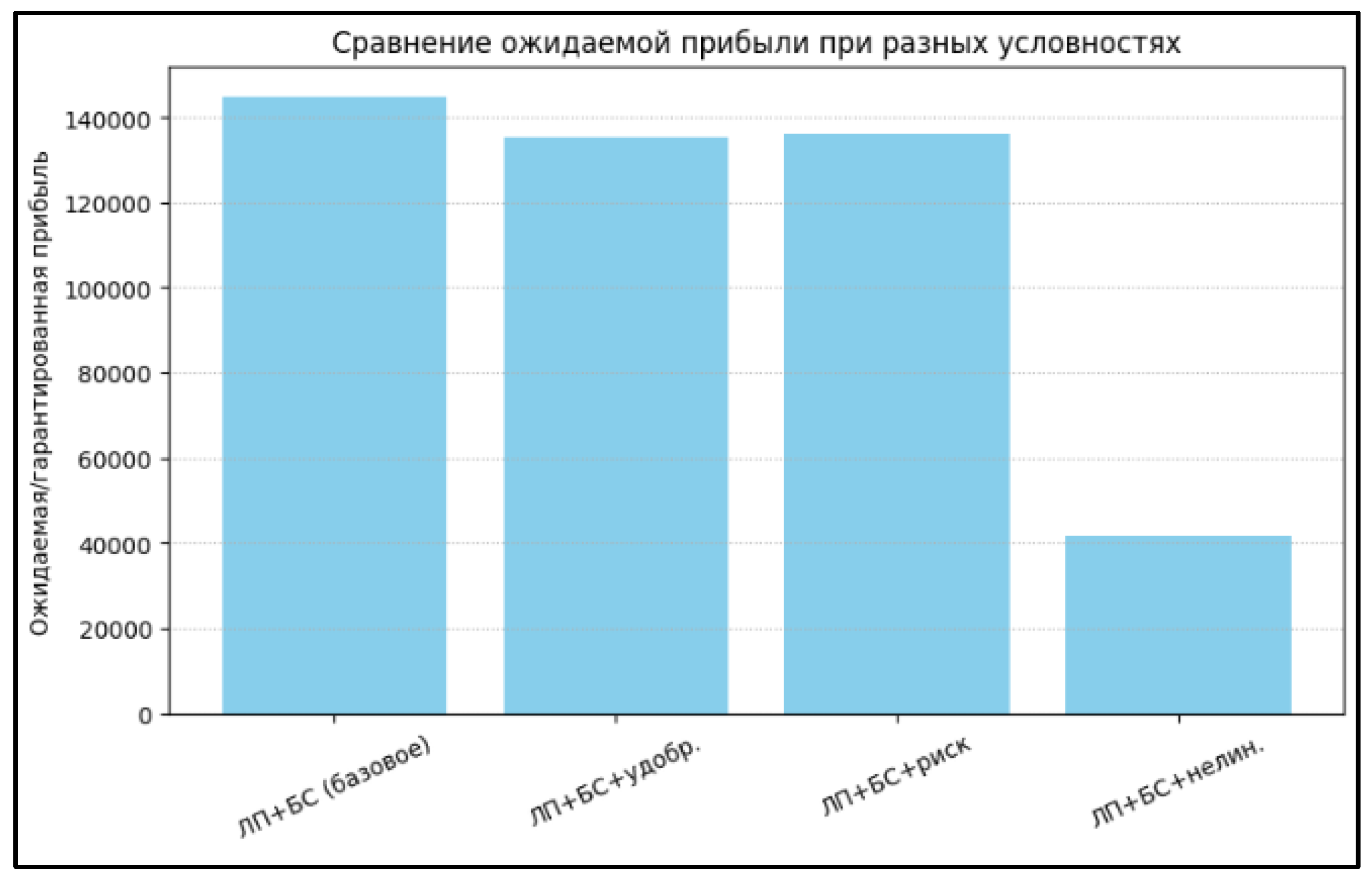
Figure 3.
Comparison of optimization approaches under complex uncertainty.
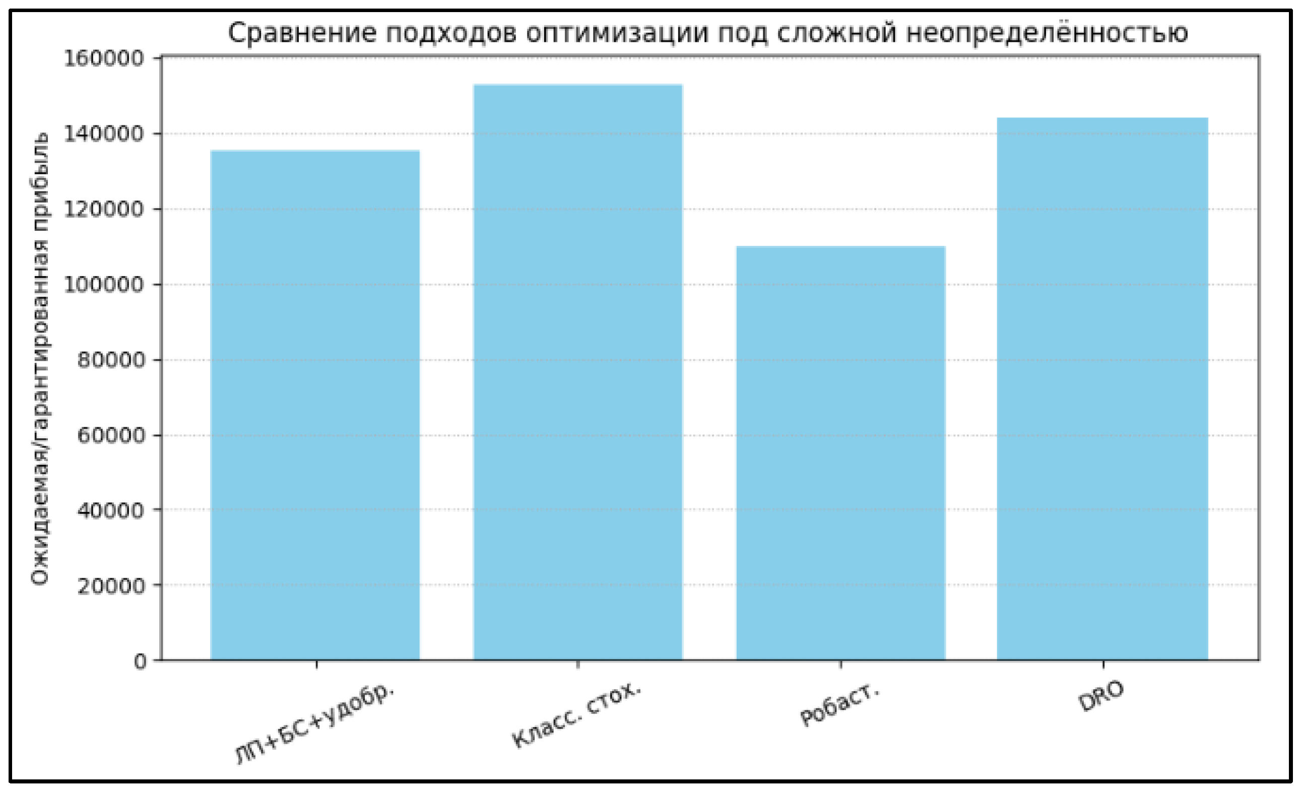

Table 1.
CPT fragment.
| № | Climate | Weather | Temperature | Precipitation | Diseases | Yield | Fertilizer costs | Global market | Demand | Price | Probability |
| 1 | Stable | Benefit. | Normal | Normal | No | High | Low | Stable | High | High. | 0.109610 |
| 2 | Stable | Good. | Extreme | Normal | No | High | Low | Stable | High | High | 0.031317 |
| 3 | Stable | Good. | Normal | Anom. | No | High | Low | Stable | High | High | 0.028417 |
| 4 | Change | Benefit. | Normal | Normal | No | High | Low | Stable | High | High | 0.027402 |
Table 2.
Fragment of the joint probability distribution.
| № | Probability | Profit_A | Profit_B |
| 1 | 0.109610 | 1980.0 | 1782.0 |
| 2 | 0.031317 | 1980.0 | 1782.0 |
| 3 | 0.028417 | 1980.0 | 1782.0 |
| 4 | 0.027402 | 1980.0 | 1782.0 |
Table 3.
Distribution and expected profit under different conditions.
| Method | A | B | Expected profit |
| LP+BN (baseline) | 10 | 0 | 144,787.79 |
| LP+BN + fertilizer restriction | 33.92 | 66.08 | 135219.64 |
| LP+BN + chance restrictions | 39.27 | 60.73 | 135995.01 |
| LP+BN + market saturation | 33.3 | 50 | 41723.82 |
Table 4.
Comparison with classical methods.
| Method | Expected profit | Nature of the solution | Complexity of implementation |
| LP+BN (proposed) | 135,219.64 | Flexible, realistic | Medium |
| Stochastic | 153000.00 | Usually one-sided | Low |
| Robust | 110,000.00 | Very conservative | Low |
| DRO | 144,000.00 | Moderately conservative | Average |
Disclaimer/Publisher’s Note: The statements, opinions and data contained in all publications are solely those of the individual author(s) and contributor(s) and not of MDPI and/or the editor(s). MDPI and/or the editor(s) disclaim responsibility for any injury to people or property resulting from any ideas, methods, instructions or products referred to in the content. |
© 2025 by the authors. Licensee MDPI, Basel, Switzerland. This article is an open access article distributed under the terms and conditions of the Creative Commons Attribution (CC BY) license (http://creativecommons.org/licenses/by/4.0/).
Copyright: This open access article is published under a Creative Commons CC BY 4.0 license, which permit the free download, distribution, and reuse, provided that the author and preprint are cited in any reuse.


