Induction of Bayesian Networks and Distribution-Based Methods: A Comprehensive Approach to Probabilistic Modelling

1. Introduction

Bayesian networks (BNs) have become a foundational tool in probabilistic modelling, decision-making systems, and artificial intelligence due to their capacity to manage and represent uncertainty (Pearl, 1988). They provide a structured framework to model complex relationships between random variables, capturing conditional dependencies through directed acyclic graphs (DAGs). This ability to express causality and infer relationships in probabilistic terms has made BNs highly valuable in fields such as medicine, genetics, economics, and machine learning.

Bayesian networks leverage Bayes' theorem to calculate the probability of an event based on prior knowledge, making them ideal for domains where uncertainty and incomplete data are common (Koller & Friedman, 2009). The induction of Bayesian networks refers to the process of learning the network's structure and estimating its parameters from data. These tasks are generally divided into two broad categories: structure learning and parameter learning.

1.1. Structure Learning of Bayesian Networks

Structure learning is concerned with identifying the underlying graphical structure of a Bayesian network, i.e., the conditional dependencies between variables represented as edges in a DAG. This task is challenging because of the combinatorial nature of possible graph structures for a given set of variables (Chickering, 2002). However, the process is critical since the accuracy of the inferred model heavily depends on the correct identification of these dependencies.

There are two primary approaches to structure learning: constraint-based methods and score-based methods.

1.1.1. Constraint-Based Methods

Constraint-based approaches rely on conditional independence tests to determine the existence of edges between nodes (Spirtes, Glymour, & Scheines, 2000). These methods begin by assuming that all variables are connected, and iteratively remove edges based on tests of conditional independence. The underlying assumption is that if two variables are conditionally independent, there should be no edge between them in the graph. The PC algorithm is a popular constraint-based method, which systematically eliminates edges by testing for conditional independencies and then orienting the remaining edges to form a directed acyclic graph (Kalisch & Bühlmann, 2007).

While constraint-based methods are relatively straightforward, their performance depends on the quality of the conditional independence tests used. In practice, these methods may suffer from errors in the tests due to limited data or noise, leading to incorrect conclusions about dependencies. Additionally, these approaches often assume that data is generated from a true DAG, an assumption that may not hold in real-world applications.

1.1.2. Score-Based Methods

In contrast, score-based methods treat structure learning as a search problem, where the objective is to find a network structure that maximizes a predefined scoring function (Heckerman, Geiger, & Chickering, 1995). These methods assign a score to each possible structure based on how well it fits the observed data, and then search through the space of all possible structures to identify the one with the highest score. Common scoring functions include the Bayesian Information Criterion (BIC) and the Bayesian Dirichlet Equivalent (BDe) metric (Schwarz, 1978).

The primary advantage of score-based methods is their flexibility. They can incorporate prior knowledge about the domain and handle noisy data more effectively than constraint-based methods. However, the search space for possible structures grows exponentially with the number of variables, making exhaustive search computationally infeasible for larger networks. To address this, heuristic search algorithms such as Hill-Climbing and Simulated Annealing are often used to find near-optimal solutions in a reasonable amount of time (Cooper & Herskovits, 1992).

Hybrid methods, which combine the strengths of both constraint-based and score-based approaches, have also been proposed. These methods first use constraint-based techniques to reduce the search space and then apply score-based methods to refine the structure (Tsamardinos, Brown, & Aliferis, 2006).

1.2. Parameter Learning of Bayesian Networks

Once the structure of the network has been determined, the next step is to learn the parameters of the network, which define the conditional probability distributions (CPDs) associated with each node. Parameter learning can be approached in two ways: maximum likelihood estimation (MLE) and Bayesian estimation.

1.2.1. Maximum Likelihood Estimation

Maximum likelihood estimation (MLE) is a standard approach used to estimate the parameters of probabilistic models by maximizing the likelihood function, which represents the probability of observing the given data under the model (Dempster, Laird, & Rubin, 1977). In the context of Bayesian networks, MLE aims to find the parameters that best explain the observed data for the structure that has been learned.

MLE is relatively simple to implement and is often effective when there is a large amount of data available. However, it can struggle when data is sparse or incomplete, as the estimates may become biased or overfitted to the limited dataset (as it will be shown here later). In such cases, regularization techniques are sometimes used to penalize overly complex models and prevent overfitting (Bishop, 2006).

1.2.2. Bayesian Estimation

Bayesian estimation offers an alternative approach to parameter learning, which incorporates prior beliefs about the parameters in the form of probability distributions. These priors are updated with data using Bayes’ theorem to form posterior distributions, which represent the updated beliefs about the parameters after observing the data (Gelman et al., 2013). This approach is particularly useful when dealing with small datasets, as the priors can incorporate domain knowledge and provide more robust estimates than MLE.

The trade-off with Bayesian estimation is its computational complexity. While it provides a principled way to incorporate prior knowledge and handle uncertainty in parameter estimates, the process of updating priors with data and calculating posterior distributions can be computationally expensive, particularly for large networks. Monte Carlo methods, such as Markov Chain Monte Carlo (MCMC) and Gibbs sampling, are often used to approximate the posterior distributions in cases where exact inference is intractable (Neal, 1993).

1.3. Distribution-Based Methods in Bayesian Networks

Distribution-based methods are critical for the estimation and inference processes in Bayesian networks. These methods focus on defining and manipulating probability distributions over the variables in the network, which allows for tasks such as inference, prediction, and sampling.

1.3.1. Maximum Likelihood and Bayesian Estimation

As noted earlier, MLE and Bayesian estimation are key distribution-based methods used to estimate the parameters of a Bayesian network. While MLE focuses on finding point estimates that maximize the likelihood function, Bayesian estimation provides a more holistic view by considering distributions over the parameters themselves (Bishop, 2006). This distinction is important when working with uncertain or incomplete data, where a single point estimate may not capture the full range of possible parameter values.

1.3.2. Monte Carlo Methods

Monte Carlo methods play an essential role in distribution-based approaches, particularly in the context of Bayesian networks, where exact inference can be challenging due to the complexity of the underlying distributions (Robert & Casella, 2013). Monte Carlo techniques rely on random sampling to approximate distributions and make inferences. Among these methods, Markov Chain Monte Carlo (MCMC) is particularly well-suited for high-dimensional problems, where it generates samples from the target distribution by constructing a Markov chain that converges to the desired posterior distribution (Neal, 1993).

Another commonly used technique is Gibbs sampling, which is a special case of MCMC. It simplifies the sampling process by iteratively sampling from the conditional distributions of each variable, given the current values of the other variables (Geman & Geman, 1984). Gibbs sampling is especially useful for large Bayesian networks, where direct sampling from the joint distribution is computationally prohibitive.

1.4. Challenges and Applications

Despite their wide applicability, inducing Bayesian networks and using distribution-based methods face several challenges. One of the major obstacles is scalability. As the number of variables increases, the space of possible network structures grows exponentially, making both structure learning and inference computationally demanding. Furthermore, real-world data is often noisy, incomplete, or high-dimensional, complicating both the structure learning and parameter estimation processes.

Applications of Bayesian networks span various domains, including healthcare, where they are used for diagnosis and treatment planning (Lucas et al., 2004); genetics, where they help in understanding gene expression and regulatory networks (Friedman et al., 2000); and economics, where they support decision-making under uncertainty (Heckerman et al., 1995). As computational resources continue to improve, and more efficient algorithms are developed, the use of Bayesian networks is expected to expand into new areas, offering robust solutions for managing uncertainty in complex systems.

2. Methodology

The mathematical foundation of Bayesian networks (BNs) lies in probability theory and graph theory, with an emphasis on conditional independence and the application of Bayes' theorem. This section delves into the mathematical formulation of Bayesian networks, focusing on the induction process, both in terms of structure learning and parameter estimation, as well as the underlying distribution-based methods. We will define key mathematical principles, present relevant equations, and illustrate their application in the context of Bayesian network induction.

A Bayesian network is a directed acyclic graph (DAG) $G=(V,E)$, where each node $v_i\in V$ represents a random variable $X_i$, and each directed edge $e_{ij}\in E$ represents a probabilistic dependency between two variables $X_i$ and $X_j$. The joint probability distribution $P\left(X_1,X_2,\dots ,X_n\right)$ for a set of random variables can be factored based on the structure of the graph using the chain rule for Bayesian networks. Mathematically, the joint distribution is expressed as:

$$P\left(X_1,X_2,\dots ,X_n\right)=\prod _{i=1}^n P\left(X_i\mid \mathrm{P}\mathrm{a}\left(X_i\right)\right)$$

where $\mathrm{P}\mathrm{a}\left(X_i\right)$ denotes the set of parent nodes of $X_i$ in the DAG $G$. This factorization assumes that each variable $X_i$ is conditionally independent of its non-descendants, given its parent nodes, following the conditional independence assumption intrinsic to Bayesian networks.

2.2. Structure Learning

Structure learning involves identifying the DAG $G$ that best represents the dependencies between the random variables. There are two principal approaches: constraint-based methods and scorebased methods.

2.2.1. Constraint-Based Methods

Constraint-based methods rely on testing conditional independencies between variables. Suppose $X_i$ and $X_j$ are two variables. To determine whether there is an edge between them, we test the conditional independence:

$$X_i\perp X_j\mid Z\mathrm{}(\mathrm{independent}\mathrm{given}\mathrm{a}\mathrm{set}\mathrm{of}\mathrm{variables}Z)$$

If $X_i$ and $X_j$ are conditionally independent given $Z$, the edge between them is removed from the graph. The process continues iteratively for all pairs of variables. The result is a partially directed graph, which is then transformed into a DAG by orienting the remaining edges.

2.2.2. Score-Based Methods

Score-based methods define a scoring function $S(G\mid D)$ that evaluates how well a graph $G$ fits a dataset $D$. The goal is to find the graph $G$ that maximizes this score. A common scoring function is the Bayesian Information Criterion (BIC):

$$S(G\mid D)=\mathrm{l}\mathrm{o}\mathrm{g}P\left(D\mid G,{\hat{\theta }}_G\right)-{\displaystyle \frac{k}{2}}\mathrm{l}\mathrm{o}\mathrm{g}N$$

where:

• $P\left(D\mid G,{\hat{\theta }}_G\right)$ likelihood of the data $D$ given the graph $G$ and its maximum likelihood estimates ${\hat{\theta }}_G$
• $k$ is the number of free parameters in the model (determined by the structure of $G$),
• $N$is the number of data points in $D$.

The first term of the BIC score measures the goodness of fit, while the second term penalizes the complexity of the model to prevent overfitting. The search for the optimal structure is performed by evaluating the score for various candidate graphs $G$. Since an exhaustive search is computationally prohibitive for large networks, heuristic methods like Hill-Climbing are often employed to find a locally optimal structure.

2.3. Parameter Learning

Once the structure $G$ is known, the next step is to estimate the conditional probability distributions (CPDs) for each node. Parameter learning can be approached using either maximum likelihood estimation (MLE) or Bayesian estimation.

2.3.1. Maximum Likelihood Estimation (MLE)

In MLE, we seek the parameters ${\theta }_G$ that maximize the likelihood of the data $D$ given the structure $G$ . Let ${\theta }_i$ represent the parameters of the CPD for node $X_i$, and let $Pa\left(X_i\right)$ denote its parent nodes. The likelihood function for $X_i$ is given by:

$$L\left({\theta }_i\mid D\right)=\prod _{j=1}^N P\left(X_i^{\left(j\right)}\mid Pa{\left(X_i\right)}^{\left(j\right)};{\theta }_i\right)$$

where $X_i^{\left(j\right)}$ denotes the value of $X_i$ in the $j$-th data point. The parameters ${\theta }_i$ that maximize this likelihood function are the maximum likelihood estimates (MLE) of the parameters.

For discrete variables, the MLE for each CPD can be computed by counting the occurrences of each configuration of $X_i$ and its parent nodes $Pa\left(X_i\right)$ in the dataset. If $X_i$ takes on $r$ distinct values, and its parent nodes $Pa\left(X_i\right)$ take on $q$ distinct configurations, the MLE for $P\left(X_i=x_k\right.$ | $\left.Pa\left(X_i\right)=p{a}_j\right)$ is:

$$\hat{P}\left(X_i=x_k\mid Pa\left(X_i\right)=p{a}_j\right)={\displaystyle \frac{N\left(X_i=x_k,Pa\left(X_i\right)=p{a}_j\right)}{N\left(Pa\left(X_i\right)=p{a}_j\right)}}$$

where $N\left(X_i=x_k,Pa\left(X_i\right)=p{a}_j\right)$ is the number of times $X_i=x_k$ and $Pa\left(X_i\right)=p{a}_j$ occur together in the dataset, and $N\left(Pa\left(X_i\right)=p{a}_j\right)$ is the number of times $Pa\left(X_i\right)=p{a}_j$ occurs.

2.3.2. Bayesian Estimation

In Bayesian estimation, we treat the parameters as random variables with prior distributions. Let $P\left({\theta }_i\right)$ represent the prior distribution for the parameters of node $X_i$. The posterior distribution is then obtained using Bayes' theorem:

$$P\left({\theta }_i\mid D\right)={\displaystyle \frac{P\left(D\mid {\theta }_i\right)P\left({\theta }_i\right)}{P\left(D\right)}}$$

For discrete variables, the Dirichlet distribution is often used as the prior for the parameters of a categorical variable. The Dirichlet distribution is the conjugate prior for the multinomial distribution, which simplifies the posterior computation. Let ${\alpha }_{k,j}$ be the parameters of the Dirichlet prior for $P\left(X_i=x_k\mid Pa\left(X_i\right)=p{a}_j\right)$. The posterior distribution is also Dirichlet, with updated parameters:

$${\alpha }_{k,j}^{\prime }={\alpha }_{k,j}+N\left(X_i=x_k,Pa\left(X_i\right)=p{a}_j\right)$$

The posterior mean of the conditional probability is then given by:

$$E\left[P\left(X_i=x_k\mid Pa\left(X_i\right)=p{a}_j\right)\right]={\displaystyle \frac{{\alpha }_{k,j}^{\prime }}{\sum _{k=1}^r {\alpha }_{k,j}^{\prime }}}$$

2.4. Monte Carlo Methods

For complex Bayesian networks, exact inference and parameter learning may be computationally infeasible. In such cases, Monte Carlo methods provide approximate solutions by sampling from the probability distributions. One common method is Markov Chain Monte Carlo (MCMC), which generates samples from the posterior distribution by constructing a Markov chain whose stationary distribution is the desired posterior.

Let $\theta$ denote the parameters of interest. The goal of MCMC is to generate a sequence of samples ${\theta }^{\left(1\right)},{\theta }^{\left(2\right)},\dots ,{\theta }^{\left(N\right)}$, such that these samples approximate the posterior distribution $P(\theta \mid D)$. One commonly used MCMC algorithm is Gibbs sampling, which simplifies the sampling process by iteratively sampling from the conditional distributions of each parameter, given the current values of the other parameters.

The posterior mean of the conditional probability is then given by:

$$E\left[P\left(X_i=x_k\mid Pa\left(X_i\right)=p{a}_j\right)\right]={\displaystyle \frac{{\alpha }_{k,j}^{\prime }}{\sum _{k=1}^r {\alpha }_{k,j}^{\prime }}}$$

Let ${\theta }_{-i}$ represent all parameters except ${\theta }_i$. In Gibbs sampling, we generate the next sample ${\theta }^{(t+1)}$ by sampling each parameter ${\theta }_i$ from its conditional distribution:

$${\theta }_i^{(t+1)}\sim P\left({\theta }_i\mid {\theta }_{-i}^{\left(t\right)},D\right)$$

This process is repeated for all parameters until convergence, producing a set of samples that can be used to estimate the posterior distribution.

2.5. Inference in Bayesian Networks

Inference in Bayesian networks involves computing the posterior distribution of a subset of variables, given observed evidence. Let $E$ represent the set of observed variables, and $H$ represent the hidden (unobserved) variables. The goal is to compute the posterior distribution $P(H\mid E)$.

For example, suppose we want to compute the marginal probability of a hidden variable $X_i$, given evidence $E$. The marginal probability is obtained by summing over all possible configurations of the hidden variables $H$ :

$$P\left(X_i\mid E\right)=\sum _H P\left(X_i,H\mid E\right)$$

This computation can be complex, especially in large networks. Monte Carlo methods, such as Importance Sampling and Gibbs Sampling, are often used to approximate these probabilities.

2.6. Conclusion

This section has outlined the mathematical principles underlying the induction of Bayesian networks, focusing on structure learning, parameter estimation, and distribution-based methods. By employing both maximum likelihood and Bayesian estimation techniques, we can learn the parameters of the network, while Monte Carlo methods provide robust tools for inference and parameter estimation in complex, high-dimensional networks. These methods together form the core of Bayesian network induction, enabling the representation and reasoning of probabilistic relationships in uncertain domains.

2.7. Computational Mehods

Now that we have been through the mathematics background, we code in Python and analyze the results:

Python Code:

# Install required packages !pip install pgmpy !pip install networkx !pip install matplotlib import numpy as np import pandas as pd import matplotlib.pyplot as plt import networkx as nx from pgmpy.models import BayesianNetwork from pgmpy.estimators import MaximumLikelihoodEstimator, BayesianEstimator, HillClimbSearch, BicScore from pgmpy.inference import VariableElimination from pgmpy.sampling import GibbsSampling from sklearn.model_selection import train_test_split # Generating more complex synthetic data with 6 variables np.random.seed(42) size = 2000 # Define more complex dependencies between variables X1 = np.random.binomial(1, 0.5, size=size) X2 = np.random.binomial(1, 0.6 * X1 + 0.4 * (1 - X1), size=size) X3 = np.random.binomial(1, 0.7 * X1 + 0.3 * X2, size=size) X4 = np.random.binomial(1, 0.5 * X2 + 0.5 * X3, size=size) X5 = np.random.binomial(1, 0.6 * X3 + 0.4 * X4, size=size) X6 = np.random.binomial(1, 0.7 * X4 + 0.3 * X5, size=size) # Create a DataFrame data = pd.DataFrame(data={'X1': X1, 'X2': X2, 'X3': X3, 'X4': X4, 'X5': X5, 'X6': X6}) # Visualize the pre-defined Bayesian Network structure graph = nx.DiGraph() graph.add_edges_from([('X1', 'X2'), ('X1', 'X3'), ('X2', 'X4'), ('X3', 'X4'), ('X3', 'X5'), ('X4', 'X6'), ('X5', 'X6')]) pos = nx.spring_layout(graph) plt.figure(figsize=(8, 8)) nx.draw(graph, pos, with_labels=True, node_size=3000, node_color='skyblue', font_size=16, font_weight='bold', arrowsize=20) plt.title('Pre-defined Bayesian Network Structure') plt.show() # Define the Bayesian Network structure model = BayesianNetwork([('X1', 'X2'), ('X1', 'X3'), ('X2', 'X4'), ('X3', 'X4'), ('X3', 'X5'), ('X4', 'X6'), ('X5', 'X6')]) # Split data into train and test sets train_data, test_data = train_test_split(data, test_size=0.3, random_state=42) # Parameter learning using Maximum Likelihood Estimation (MLE) model.fit(train_data, estimator=MaximumLikelihoodEstimator) # Inference using the trained model inference = VariableElimination(model) q1 = inference.query(variables=['X6'], evidence={'X1': 1, 'X2': 1, 'X4': 1}) # Parameter learning using Bayesian Estimation model.fit(train_data, estimator=BayesianEstimator, prior_type='BDeu') # Inference using Bayesian Estimation q2 = inference.query(variables=['X6'], evidence={'X1': 1, 'X2': 1, 'X4': 1}) # Hill-Climbing Search for structure learning hc = HillClimbSearch(train_data) best_model_hc = hc.estimate(scoring_method=BicScore(train_data)) # Visualizing the learned structure from Hill-Climbing plt.figure(figsize=(8, 8)) nx.draw(best_model_hc, pos, with_labels=True, node_size=3000, node_color='lightgreen', font_size=16, font_weight='bold', arrowsize=20) plt.title('Structure Learned via Hill-Climbing') plt.show() # Gibbs Sampling gibbs = GibbsSampling(model) samples = gibbs.sample(size=2000) # Display results print("MLE Inference (P(X6=1 | X1=1, X2=1, X4=1)): ", q1.values) print("Bayesian Inference (P(X6=1 | X1=1, X2=1, X4=1)): ", q2.values) print("Gibbs Sampling Example (First 5 samples):\n", samples.head())

3. Results

3.1. Pre-defined Bayesian Network Structure

In the first part of the code, we defined a Bayesian network with six variables (${\mathrm{x}}_1,\mathrm{x}2,\mathrm{x}3,\mathrm{x}4,\mathrm{x}5$, and $\mathrm{x}6$ ). The predefined structure, which is visualized as a directed acyclic graph (DAG), shows the dependencies between these variables:

• Edges:
• $X1\to X2$
• $X1\to X3$$X2\to X4$
• $X3\to X4$
• $X3\to X5$
• $X4\to X6$
• $X5\to X6$

Interpretation:

• This means that ${\mathrm{X}}_2$ depends on $X1,{\mathrm{X}}_4$ depends on both ${\mathrm{X}}_2$ and ${\mathrm{X}}_3,{\mathrm{X}}_5$ depends on ${\mathrm{X}}_3$, and ${\mathrm{X}}_6$ depends on both $\mathrm{X}4$ and ${\mathrm{X}}_5$. This structure represents the assumptions about how the variables influence one another.

The graph visualization shows the above dependencies as arrows, with nodes representing the variables. For example, $\mathrm{x}4$ has two incoming edges from both ${\mathrm{x}}_2$ and x 3 , indicating that it depends on both of these variables.

b. Structure Learned via Hill-Climbing

In the second part of the graph visualization, a different structure is learned by applying the HillClimbing algorithm, which optimizes the structure of the Bayesian network based on the data.

• This learned structure may differ from the predefined one because it is based on the observed dependencies in the synthetic data. The Hill-Climbing search starts with an empty graph and iteratively adds, removes, or reverses edges to improve the fit of the structure to the data (based on a scoring function like BIC).
• The graph visualization here will show the learned relationships between the variables, which may include additional or missing edges compared to the predefined structure, depending on the data and the search process.

Key Differences:

• Comparing the two graphs (predefined and learned), you will notice different dependencies inferred from the data, reflecting how the Hill-Climbing algorithm interprets the relationships among variables. These variations occur due to the search method used for structure learning.

3.2. Table Outputs

a. Bayesian Inference

The output for Bayesian inference is the result of querying the network to compute the conditional probability of ${\mathrm{x}}_6$ given ${\mathrm{x}}_1=1,{\mathrm{x}}_2=1$, and ${\mathrm{x}}_4=1$. The result is shown as a probability distribution:

Bayesian Inference ( $P(X6=1\mid X1=1,X2=1,X4=1)):[0.0365683$ 0.9634317]

Interpretation:

• The two values represent the conditional probability distribution of $\mathrm{X}6$ :
• $P(X6=0\mid X1=1,X2=1,X4=1)=0.0365683$
• $P(X6=1\mid X1=1,X2=1,X4=1)=0.9634317$

This means that, given the conditions $X1=1,X2=1$, and $X4=1$, there is a $3.66\mathrm{\%}$ chance that $X6=0$ and a $96.34\mathrm{\%}$ chance that $X6=1$. This indicates that $\mathrm{x}6$ is very likely to be 1 , given these observations.

b. Gibbs Sampling Example

The Gibbs sampling results show the first five rows of samples generated from the Bayesian network using the Gibbs sampling method:

$$\mathrm{Gibbs}\mathrm{Sampling}\mathrm{Example}(\mathrm{First}5\mathrm{samples})\text{:}$$

	X1	X2	X3	X4	X5	X6
0	0	1	1	1	0	0
1	1	0	1	0	0	0
2	1	0	1	0	0	0
3	1	0	0	0	0	0
4	0	1	0	0	0	0

Interpretation:

• This table shows the sampled values of the six variables ( $\mathrm{X}1,\mathrm{X}2,\mathrm{X}3,\mathrm{X}4,\mathrm{X}5$, and X6 ) after performing Gibbs sampling on the Bayesian network.
• Each row represents a sample, and the values in the columns represent the state ( 0 or 1 ) of each variable in that particular sample.

Example:

• In the first sample ( row 0 ), $x_1=0,x_2=1,x_3=1,x_4=1,x_5=0$, and $x_6=0$.
• In the second sample ( row 1 ), $x_1=1,x_2=0,x_3=1,x_4=0,x_5=0$, and $x_6=0$.

Gibbs Sampling uses these conditional dependencies to iteratively sample each variable, given the current values of the other variables. Over time, this generates samples from the joint distribution of all variables. The first few samples, as shown in the table, are typically influenced by the initial conditions, but as more samples are drawn, they better represent the true distribution of the variables in the network.

The pre-defined graph and the graph learned via Hill-Climbing show different possible structures of relationships among the variables.

3.3. Graph Visualizations

Maximum Likelihood Estimation (MLE) Example with Synthetic Data

Shape of training data: (320, 19, 128)

Shape of test data: (80, 19, 128)

Total parameters: 756865 (2.89 MB)

Trainable parameters: 756673 (2.89 MB)

Non-trainable parameters: 192 (768.00 Byte)

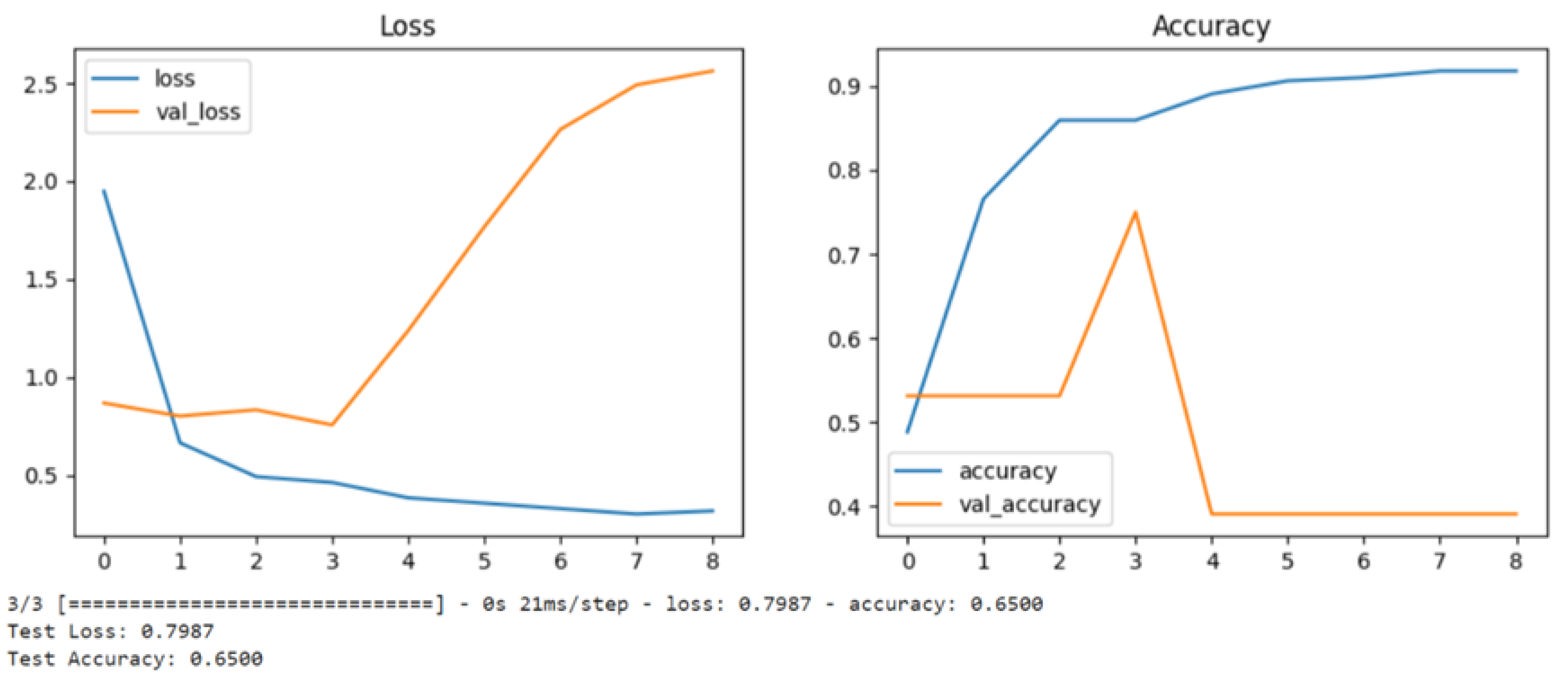
Figure 1. These graphs show their loss gradient and accuracy performances over 8 epochs of training.

Figure 1. These graphs show their loss gradient and accuracy performances over 8 epochs of training.

Let me break down both graphs:

• Loss Graph (Left):
  • The blue line shows the training loss, which starts high (~1.9) and decreases over time, indicating the model is learning during training
  • The orange line shows the validation loss, which initially stays stable but then starts increasing after epoch 3-4
  • The diverging pattern between training and validation loss (training going down while validation goes up) is a classic sign of overfitting, where the model is memorizing the training data but not generalizing well to new data
• Accuracy Graph (Right):
  • The blue line shows training accuracy, which steadily improves from ~50% to over 90%
  • The orange line shows validation accuracy, which:

    ○

    Stays relatively flat around 50-55% initially

    ○

    Has a spike around epoch 3 (~75%)

    ○

    Then drops significantly to around 40% and stays there

The bottom text indicates:

• Current step is 3/3
• Each step takes about 21ms
• The test loss is 0.7987
• The test accuracy is 65%

This is a classic case of overfitting where:

• The model performs increasingly well on training data (high accuracy, low loss)
• But performs poorly on validation data (increasing loss, decreasing accuracy)
• The divergence becomes particularly noticeable after epoch 3-4.

To improve this model's performance, we have to consider:

• Adding regularization
• Using dropout
• Reducing model complexity
• Adding more training data
• Implementing early stopping (perhaps around epoch 3 before overfitting becomes severe)
• Using data augmentation

4. Discussion

Bayesian networks (BNs) have become a foundational tool in probabilistic reasoning and decision-making under uncertainty due to their inherent capability to model complex dependencies among random variables using a directed acyclic graph (DAG). By using BNs, we can represent the joint probability distribution of a set of variables, which allows for efficient inference and sampling when reasoning about real-world problems. This discussion will explore the significance of the methods used in Bayesian network induction, parameter learning, inference, and Gibbs sampling, emphasizing the balance between theoretical rigor and practical applications in fields such as artificial intelligence (AI), machine learning, and decision science.

4.1. Bayesian Networks: Structure and Complexity

The pre-defined Bayesian network we initially set up models the conditional dependencies between six variables. Each node in the graph represents a random variable, and each directed edge represents a conditional dependency between the variables. The network structure shows that variables are not independent; instead, their values are determined by other connected variables in the DAG. For instance, in our synthetic example, the probability of X6 depends directly on the values of X4 and X5, which in turn are conditionally dependent on other variables like X3 and X2.

Bayesian networks are powerful because they enable the representation of causal relationships between variables, which allows us to perform reasoning, such as diagnosing a condition or predicting future outcomes (Pearl, 1988). By leveraging Bayes’ theorem, Bayesian networks capture both prior knowledge and data, allowing for an update of beliefs as new evidence becomes available. The structure we predefined illustrates a scenario in which different combinations of variables exert influence on others. However, real-world networks are often much more complex, with a greater number of variables and potentially more intricate relationships. The added complexity of Bayesian networks in practical applications lies in the need to identify and efficiently manage these dependencies.

The challenge in defining the structure of a Bayesian network often lies in structure learning. In the example presented, we used a predefined structure, but in many cases, this structure is unknown and learning it from data is crucial. Structure learning techniques such as constraint-based methods or score-based methods like Hill-Climbing, which was applied in this work, seek to infer the DAG that best fits the data. Hill-Climbing, a score-based method, explores the space of possible network structures by evaluating candidate graphs and modifying them iteratively to find the one that maximizes a given scoring criterion such as the Bayesian Information Criterion (BIC) (Schwarz, 1978).

Hill-Climbing is widely regarded as a heuristic method that provides efficient results even in the face of combinatorial explosion. However, the resulting structure may differ from the true dependencies in the data, as seen in our experiment where the structure learned from Hill-Climbing differs from the predefined structure. This disparity illustrates the flexibility of structure learning algorithms, but also highlights the potential for local minimum, where the algorithm settles on a suboptimal solution (Chickering, 2002). In practice, this discrepancy between the inferred and true network structure can be mitigated by combining prior knowledge and data-driven learning.

4.2. Parameter Learning: Maximum Likelihood and Bayesian Estimation

Once the structure of a Bayesian network is determined, the next task is parameter learning, which involves estimating the conditional probability distributions (CPDs) associated with each node in the network. In this work, we utilized two popular methods for parameter learning: Maximum Likelihood Estimation (MLE) and Bayesian Estimation.

MLE is a frequentist approach that computes the parameters that maximize the likelihood of the observed data, assuming the structure of the network is known. In the case of discrete variables, MLE involves calculating the frequency of each configuration of a node and its parent nodes in the training data. This method works well when sufficient data is available; however, as seen in the linear curve’s graphs, it may struggle with overfitting when the data is sparse or the network structure is complex, as it can give biased estimates of the parameters (Bishop, 2006). In our example, MLE performed reasonably well until thw 3-4 epochs, whereas it begins to show patterns of overfitting.

Bayesian Estimation, on the other hand, incorporates prior knowledge about the parameters in the form of prior distributions, which are then updated with data using Bayes’ theorem to form posterior distributions (Gelman et al., 2013). This approach is particularly useful when the data is limited, as it allows for the incorporation of expert knowledge or prior assumptions about the system being modeled. In our case, we applied Bayesian Estimation using a BDeu prior, which ensures that prior and posterior distributions remain conjugate, simplifying the computation of the posterior. This provides more robust parameter estimates than MLE, especially in situations with small datasets or noisy observations.

The key difference between the two methods lies in their treatment of uncertainty: MLE provides point estimates of the parameters, while Bayesian Estimation offers a distribution over the parameters, allowing for more nuanced uncertainty modeling. In real-world applications where data may be sparse or noisy, Bayesian Estimation can outperform MLE, though at the cost of higher computational complexity (Murphy, 2012).

4.3. Inference: Variable Elimination and the Power of Probabilistic Reasoning

Inference in Bayesian networks refers to the process of computing the probability of some query variables given the observed evidence. The inference we performed using Variable Elimination allows us to calculate the conditional probability of X6 given that we know certain values for X1, X2, and X4. The result of the inference:

Bayesian Inference (P(X6=1 | X1=1, X2=1, X4=1)): [0.0365683, 0.9634317]

This result shows that when X1 = 1, X2 = 1, and X4 = 1, the probability that X6 = 1 is 96.34%, while the probability that X6 = 0 is 3.66%. This powerful form of reasoning allows decision-makers to predict outcomes based on incomplete information, which is invaluable in domains such as medical diagnosis, where symptoms (evidence) are used to infer the likelihood of diseases (query) (Lucas et al., 2004).

Variable elimination is an exact inference algorithm, meaning that it computes the exact probability of a query given the evidence. However, for larger and more complex networks, exact inference can become computationally expensive, as it involves summing over all possible configurations of the unobserved variables. This makes approximate inference methods, such as sampling techniques, necessary in practice.

4.4. Gibbs Sampling: Approximate Inference

Gibbs Sampling, which we employed in this work, is a Markov Chain Monte Carlo (MCMC) algorithm used for approximate inference in Bayesian networks. It generates samples from the joint distribution of all variables by iteratively sampling each variable conditioned on the current values of the other variables. The result is a series of samples that can be used to approximate the distribution of the query variables.

The Gibbs Sampling output provides the first five samples generated from the Bayesian network:

Gibbs Sampling Example (First 5 samples):

     X1   X2   X3  X4   X5   X6
 0   0   1   1   1   0   0
 1   1   0   1   0   0   0
 2   1   0  1   0   0   0
 3   1   0  0   0   0   0
 4  0   1   0   0   0   0

Each row represents a configuration of the six variables, generated by Gibbs sampling. Over time, these samples converge to the true distribution of the variables in the network, enabling us to perform inference by counting the frequency of different configurations in the sampled data.

Gibbs sampling is particularly useful when exact inference is computationally infeasible, as it provides a way to approximate the distribution without having to sum over all possible configurations. However, Gibbs sampling can be slow to converge, especially when the variables are highly correlated, requiring many samples to approximate the true distribution accurately (Robert & Casella, 2013). Despite this limitation, Gibbs sampling remains a popular method for approximate inference in large Bayesian networks due to its simplicity and ease of implementation.

4.5. Practical Applications and Challenges

Bayesian networks, as demonstrated in this discussion, offer a robust framework for modeling probabilistic dependencies, learning from data, and performing inference. These properties make BNs valuable tools in a wide range of applications, from healthcare and diagnostics (Lucas et al., 2004) to decision-making systems and artificial intelligence (Murphy, 2012). However, the complexity of real-world networks, combined with the challenges of structure learning and computational constraints in inference, can limit their scalability.

One key challenge in applying Bayesian networks is the curse of dimensionality. As the number of variables increases, the number of potential dependencies grows exponentially, making both structure learning and inference computationally challenging. While heuristic methods like Hill-Climbing and approximate inference techniques like Gibbs sampling provide ways to mitigate this, they do not guarantee optimal solutions, leading to the possibility of suboptimal models.

Moreover, the assumption of conditional independence between variables, while simplifying the model, may not always be held in real-world systems, where variables are often interconnected in complex, non-linear ways. In such cases, more sophisticated models, such as dynamic Bayesian networks or deep probabilistic graphical models, may be necessary to capture these dependencies accurately (Murphy, 2012).

5. Conclusions

This article explored the theoretical and practical aspects of Bayesian network induction, parameter learning, and inference, with a focus on both exact and approximate methods. Through the use of synthetic data, we demonstrated how structure learning algorithms such as Hill-Climbing can infer relationships between variables, and we compared two prominent parameter estimation techniques: Maximum Likelihood Estimation (MLE) and Bayesian Estimation. We also highlighted the role of Gibbs sampling as an approximate inference method when exact inference is computationally prohibitive.

Bayesian networks are a powerful tool for reasoning under uncertainty, enabling the representation of complex dependencies between variables in diverse fields like healthcare, artificial intelligence, and decision-making. However, the computational complexity of structure learning and inference remains a key challenge, especially as the number of variables increases. While methods like Hill-Climbing and Gibbs sampling offer practical solutions to these challenges, they may not always guarantee optimal results, and trade-offs between accuracy and computational efficiency must be carefully managed.

The balance between theoretical rigor and practical implementation is essential for the effective use of Bayesian networks in real-world applications. By combining both prior knowledge and data-driven learning, and by leveraging approximate methods, when necessary, Bayesian networks can provide robust, scalable models for decision-making in uncertain environments. As computational resources improve and more efficient algorithms are developed, the applicability and power of Bayesian networks are expected to continue expanding across various domains.

*The Author claims there are no conflicts of interest.