
Submitted:
28 October 2025
Posted:
30 October 2025
You are already at the latest version
Abstract
As devices and systems shrink in size, understanding heat transfer at the mesoscopic scale becomes increasingly critical for the design of efficient thermal management strategies. This study investigates convective heat transfer in concentric cylinders, a geometry which is relevant to small-scale technologies. Finite elements simulation are used to examine the influence of geometry and temperature on effective thermal conductivity, and on a parameter introduced as the apparent thermal transfer coefficient. It is found that the effective thermal conductivity goes above unity for inner and outer radii at the millimeter scale, which is smaller than that predicted by previous analytical studies. This deviation is attributed to the fact that finite element simulations capture the behavior of temperature boundary layers more accurately at small scales than analytical models. These insights aid in identifying conditions in which convection can be ignored, significantly simplifying thermal simulations. This work also reveals that at mesoscales, the ratio between outer and inner radius for which a cylinder can be considered free-standing, is much larger than at the macroscale. This highlights the importance of taking the surrounding surfaces into consideration when performing experiments on the heat transfer properties of mesoscale cylinders such as wires.
Keywords:
finite element
; concentric cylinders
; small-scale
; simulation
; fluid
1. Introduction
Heat transfer between concentric cylinders, also known as annuli, has been extensively studied at the macro scale. In 1975, Raithby and Hollands published seminal work that has become the reference work for the theory of convective heat loss for various geometries, including concentric cylinders [1,2]. Their result is expressed by the following equation:
where q is the heat transfer rate per cylinder length, and and are the temperatures on the inner and outer cylinders respectively. and are the radius of the inner and outer cylinders, and is the effective thermal coefficient of the fluid. This equation is very similar to the exact solution to the concentric cylinder geometry for conductive heat transfer, which can be shown to be:
The key parameter change is k, which is the regular thermal conductivity of the fluid. The relation between k and given by the empirical equation
Since the convective heat transfer rate should not be less than the conductive-only heat transfer rate, if Equation 3 yields a result less than one. Furthermore, is the Prandtl number and is the Rayleigh number for the concentric cylinder geometry
where g is the gravitational acceleration, is the volumetric thermal expansion coefficient, is the kinematic viscosity and is the thermal diffusivity of the fluid. The length scale parameter is given by
It can be seen that scales linearly with the absolute size of , with a less straightforward relation to the relative size of to . The concentric cylinder geometry is shown schematically in Figure 1a), and a plot of as predicted by Equation 3 is shown in Figure 1b).
Raithby and Hollands found that Equation 3 holds for a wide range of , relating the equation to the previous experimental studies using air as the fluid by Beckmann, and Grigull and Hauf [3,4].
Although only the temperature difference between and enters into equations 1 and 4, their absolute values matters indirectly through temperature dependent material parameters. Thus for a given fluid, three experimental parameters can be used to vary : , , and . The experimental data originally used to verify Equation 3 fit well for . Since a low might entail either a small temperature difference and/or a small geometry, one might assume that this means Equation 3 holds for small scales, as long as continuum equations hold. However, this assumption would be incorrect: The experimental data relied chiefly on varying through , and , with never being below –1. Thus, for small scales with air as the fluid medium, the correlation for has not been tested.
At the same time, in the development of Equation 3, Raithby and Holland assumed that the radial temperature profile in a concentric cylinder geometry can be divided into three parts: two boundary layers close to the surfaces, where the temperature changes rapidly, and one intermediate layer, where the temperature does not change with radial distance. At small scales, estimating the size of these boundary layers becomes a chicken-and-egg issue: They are dependent on the heat flux, but the heat flux is dependent on the effective heat transfer coefficient, which is dependent on the size of the boundary layer. The behavior of in concentric cylinder geometries as and approach small scales has remained largely unexplored and, as such, remains an open question.
Heat transfer on the small scale is becoming ever more relevant, and thus there is now a need to investigate this unsolved issue. On the technological side, the development of MEMS has turned mesoscale heat transfer problems into practical issues of economic significance. On the scientific side, the ever increasing availability of nano- and microfabrication capabilities among the scientific community has led to more research on small-scale phenomena in general. Whenever this involves temperature differences, heat transfer problems become relevant as potential error sources. Such issues are typically avoided all together by performing experiments in vacuum [5,6,7].
With a better understanding of small-scale heat transfer in air, one could in some instances avoid such complicated and expensive experimental procedures. Additionally, a solid understanding of small-scale heat transfer at the continuum level helps distinguish between behaviors that fall within the continuum model and those that go beyond it.
Finally, it is relevant to the interpretation of existing experimental works on related systems. While the heat transfer properties of concentric cylinder geometries have not been experimentally examined at small scales, there are some works on the heat transfer properties of nominally free-standing micro-wires [8,9]. While these works do not examine concentric cylinders, the short distance in absolute terms between micro-wires and nearest surfaces, means that a concentric cylinder geometry can be seen as a relevant first approximation model of the experimental set-ups.
In this work, we use the finite element method to numerically investigate the influence of geometry and temperature difference on the convective heat transfer properties of concentric cylinders. Two physical models are built: one assuming conduction as the only heat transfer mechanism, and one explicitly modelling natural convection. The models are built and the heat transfer evaluated for a large range of , and . The results are then compared to those predicted by Equation 3.
2. Materials and Methods
A single concentric cylinder geometry was built, as shown in Figure 2a). The geometry consists of two half circles, with the left side using symmetry conditions, thus physically representing two full circles. To enable automatic meshing and simulation of a large number of parameter combinations, and where varied through scaling parameters:
Here, , and . scales the entire geometry, while scales the relative distance between the cylinder walls. To cover a large parametric space, and were varied exponentially with between and , and between and .
The boundary situated at is held at , while the temperature at is varied through a temperature difference parameter : , where is varied exponentially between K and K.
Based on these boundary conditions and geometries, two different two-dimensional physical simulation models were built using the commercial finite element software COMSOL. One model considered only heat transfer by conduction, using the heat transfer in solids and fluids COMSOL module. The other model also included convection by laminar flows, using both the heat transfer in solids and fluids module and the laminar flow module. The heat transfer in solids and fluids module solves the equation
where is the thickness of the system, is the density, the specific heat capacity, the translational motion and T the temperature. Q and contains additional global and local heat sources and is the thermoelastic damping. Finally, the conductive heat flux is
For the laminar flow module, the governing equations are the Navier-Stokes equations. Assuming a weakly compressible, stationary one-phase flow with no turbulence, the relevant Navier-Stokes equations become
and
Here, p is the pressure, is the identity matrix, is the dynamic viscosity, is the surface normal of the boundary, is the volume force vector, and is gravity. Gravity was applied perpendicular to the length of the cylinders.
When combining the laminar flow and heat transfer modules, the viscous heating term is added to the the right hand side of Equation 7:
The conduction-only model was meshed using only linear, triangular elements, while the convection model also made use of layers of linear rectangular elements, around the boundaries. The finest meshing settings available in COMSOL were used. For the smallest geometrical parameters, this entails minimum element size of about 80– and a maximum size of around 40–. For the largest parameter combination, it results in a minimum size of 4– and a maximum size of 2–. Generally, this results in good quality elements, with some lower quality elements around the smaller cylinder when . A plot of element quality based on skewness is given in Figure 2 b) and c).
Material parameters were imported from COMSOL’s materials library for air. The relevant parameters are all included as functions of temperature.
For each combination of parameters, a steady-state simulation was run for each of the physical models, to estimate the the heat transfer Q from the inner to the outer cylinder. Based on this, was calculated as
where is the resulting heat transfer from the convection model, while is the result from the conduction-only model.
3. Results and Discussion
Figure 3a) show the evaluated values for for all parameters combinations. It is clear that for most of the parameter space, as long as , and are sufficiently small, . This suggests that for this part of the parameter space, convection plays little role in the heat transfer.
This is qualitatively in line with the analytical model of Raithby and Hollands. To compare the quantitative predictions of as their analytical solution is plotted in Figure 3b) as a function of and compared to our results, for 100–, for three different . Our numerical results predict significantly higher than their analytical result. Put differently, our results predict that the transition from convection-dominated to conduction-dominated heat transfer happens for smaller , and than what Raithby and Hollands’ model does.
To examine the behavior of the system around the inflection point where it transitions from the conductive to the convective regime, we plot the temperature profiles along a horizontal line at for nine combinations of and , keeping 10K–K in Figure 4b). It is evident that the boundary layer is tied to : where the boundary layers are well developed, with a large region of intermediate temperature in the middle, is larger.
In Figure 4a), velocity streamlines for the same parameter combinations as in Figure 4b) are plotted. Black lines indicate equithermal lines, set 1K–K apart. By comparison with Figure 4a), it is clear that the increase in is also tied to the establishment of a “plume”.
To explore the experimental implication of these results, we define an apparent thermal transfer coefficient as
where A is the surface area of the inner cylinder, and is either the conductive or convective total heat transfer between the cylinders.
The thermal transfer coefficient is an interface property, and is thus only a meaningful concept when discussing a free-standing cylinder. On the macro scale, the regime transfer between a free-standing cylinder and concentric cylinders starts to occur more or less when [10]. However, this is not given for smaller scales. The apparent heat transfer coefficient is what one would perceive to be the thermal transfer coefficient of a cylinder of radius if measuring with a surrounding surface away.
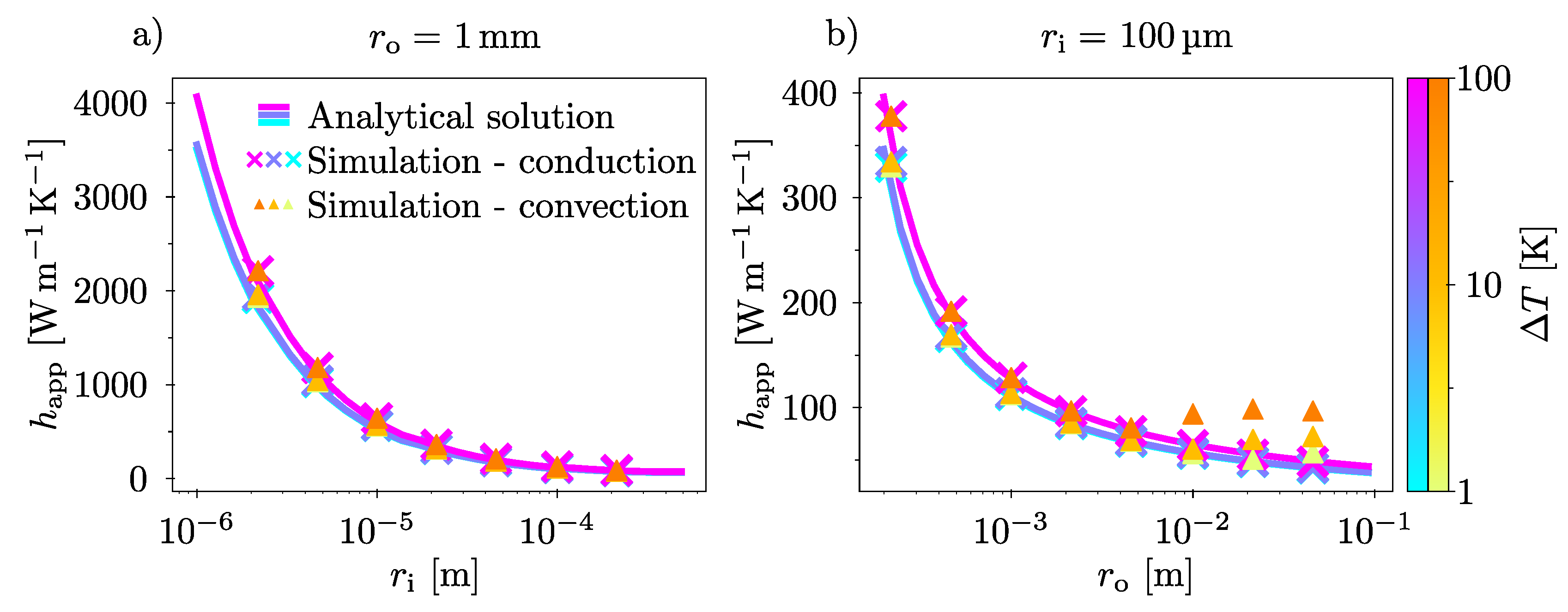
One way to determine the distance for which the transfer from a concentric cylinder regime to a free-standing wire regime occurs, is when becomes constant with increasing . In Figure 5b), is plotted for 100–. It can be seen from the convection simulation results that the apparent thermal transfer coefficient for 100– does not reach a stable level before 2– for 100K–K, and only stabilizes for even larger for lower . This implies that for a wire of 100–, the free standing regime only starts when - a very large deviation from the macro scale.
An important implication of our results is the extent to which conduction-only simulations can replicate the outcomes of convection-inclusive simulations. This finding is valuable given that convection simulations are significantly more complex and computationally demanding. If the size regimes where convection effects are negligible can be reliably identified, conduction-based simulations may serve as an efficient alternative for estimating heat transfer properties in more complex geometries.
To illustrate this point, we plot as a function of , for 1– in Figure 5a). As can be seen, the simulation model, the conduction model, and the the analytical model all yields very similar results. Furthermore, they are all able to reproduce the trends experimentally reported by Wang & Tang and by Wang et al. [8,9].
While 1– is not, perhaps, a large distance, it is certainly a magnitude that is practical to work with experimentally. Thus, although some more direct experimental comparisons might be required to confirm these numerical results, they nevertheless offer a simple solution in estimating heat loss to air for experiments on the small scale: By ensuring a surface sitting around 1– away from an experimental region of interest, one should be able to accurately model the thermal behaviour of the system without needing to include convection.
Another interesting observation is the fact that there is a point of minimum heat transfer. For a given and , it can be seen from Figure 5b) that the apparent thermal transfer coefficient in the beginning is decreasing for increasing , until it increases slightly again towards the right hand side of the graph. At the turning point, the curvature effect that causes the to increase with decreasing is not very prevalent, yet the convective properties of air have not yet become dominant. This means that for a given , there is a relatively narrow region of where the poor thermal conductivity of air can be directly utilized to make it act as a thermal insulator.
Even if the focus in this work has been on air as the fluid, it is possible to make some general conclusions as to how replacing air with another fluid would change the results presented here. Provided that the relevant properties of the replacement fluid are approximately linear over the temperature range investigated, all trends should remain the same. From this, one can use equations 3 and 4 to predict in which way a change in fluid properties would change the outcome. For instance, for a given parameter combination, a fluid with a higher kinematic viscosity would presumably have a smaller than air, all other things being equal.
4. Conclusion
This work provides a better understanding of small-scale heat transfer in air-filled concentric cylinders. Combinations of parameters where heat transfer goes from convection-dominated to conduction-dominated are identified. This transition is substantially different from what previous analytical works suggest: We find that that convection plays a role at smaller sizes and temperature differences than others have found previously. This can be explained by earlier works not properly accounting for the behaviour of temperature boundary layers at small scales. Using the finite element method, this is accounted for in our model. Thus, our work can be used in future research to identify parameter combinations where it can be safely assumed that conduction is the main heat transfer mechanism – potentially greatly simplifying modelling of heat transfer problems.
Furthermore, we illustrate for the first time the importance of accurate control of surrounding surfaces when performing small-scale heat transfer experiments. It is shown that a cylinder with a micrometer-scaled radius cannot be assumed to be freestanding unless the nearest surface is at least some hundreds of removed. This is very different from the macro-scale assumption that a cylinder is freestanding of the nearest surface is at least away.
Author Contributions
Conceptualization, TW; methodology, TW; software, TW; validation, TW; formal analysis, TW; data curation, TW; writing—original draft preparation, TW; writing—review and editing, JH, ZZ; visualization, TW; supervision, JH, ZZ; funding acquisition, JH. All authors have read and agreed to the published version of the manuscript.
Funding
The Research Council of Norway is acknowledged for the support to the Infrastructure project Norwegian Micro- and Nano-Fabrication Facility, NorFab, project no. 295864
Institutional Review Board Statement
Not applicable
Data Availability Statement
Data Availability Statement: The raw data supporting the conclusions of this article will be made available by the authors on request.
Conflicts of Interest
The authors declare no conflicts of interest.
References
- Raithby, G.; Hollands, K. A General Method of Obtaining Approximate Solutions to Laminar and Turbulent Free Convection Problems. In Advances in Heat Transfer; Elsevier, 1975; Vol. 11, pp. 265–315. [CrossRef]
- Bergman, T.L.; Lavines, A.S.; Incropera, F.P.; Dewitt, D.P. Fundamentals of Heat and Mass Transfer, 7th ed.; John Wiley & Sons, Ltd, 2011.
- Beckmann, W. Die Wärmeübertragung in zylindrischen Gasschichten bei natürlicher Konvektion. Forschung auf dem Gebiet des Ingenieurwesens A 1931, 2, 213–217. [Google Scholar] [CrossRef]
- Grigull, U.; Hauf, W. NATURAL CONVECTION IN HORIZONTAL CYLINDRICAL ANNULI. In Proceedings of the International Heat Transfer Conference 3. Begel House Inc., 1966. [CrossRef]
- Cheng, Z.; Liu, L.; Xu, S.; Lu, M.; Wang, X. Temperature Dependence of Electrical and Thermal Conduction in Single Silver Nanowire. Scientific Reports 2015, 5, 10718. [Google Scholar] [CrossRef] [PubMed]
- Lu, L.; Yi, W.; Zhang, D.L. 3ω Method for Specific Heat and Thermal Conductivity Measurements. Review of Scientific Instruments 2001, 72, 2996–3003. [Google Scholar] [CrossRef]
- Soini, M.; Zardo, I.; Uccelli, E.; Funk, S.; Koblmüller, G.; Fontcuberta i Morral, A.; Abstreiter, G. Thermal Conductivity of GaAs Nanowires Studied by Micro-Raman Spectroscopy Combined with Laser Heating. Applied Physics Letters 2010, 97, 263107. [Google Scholar] [CrossRef]
- Wang, X.; Guo, R.; Jian, Q.; Peng, G.; Yue, Y.; Yang, N. Thermal Characterization of Convective Heat Transfer in Microwires Based on Modified Steady State “Hot Wire” Method. ES Materials & Manufacturing 2019, Volume 5 (September 2019), 65–71.
- Wang, Z.L.; Tang, D.W. Investigation of Heat Transfer around Microwire in Air Environment Using 3ω Method. International Journal of Thermal Sciences 2013, 64, 145–151. [Google Scholar] [CrossRef]
- Atayılmaz, Ş.Ö. Experimental and Numerical Study of Natural Convection Heat Transfer from Horizontal Concentric Cylinders. International Journal of Thermal Sciences 2011, 50, 1472–1483. [Google Scholar] [CrossRef]
Figure 1.
a) shows a sketch of the concentric cylinder geometry, with length L approaching infinity. Note that L and are not directly related. b) shows a plot of the result in Equation 3 for air, with 273– and 283–. Notice the logarithmic range for and , going from micrometer to meter scale. The red area is where Equation 3 returns values less than one, which can be interpreted as the model predicting that there is only conduction, no convection.
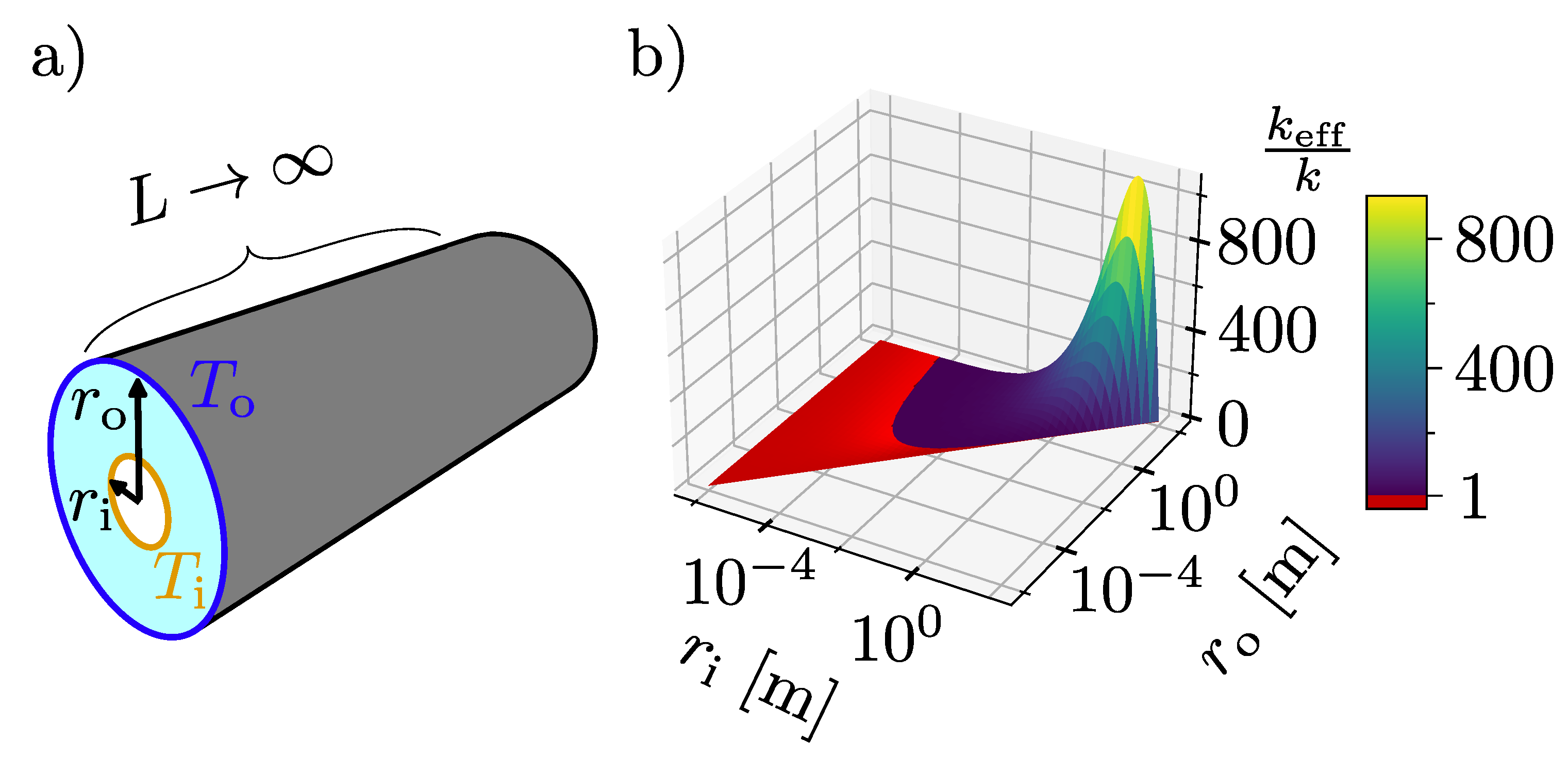
Figure 2.
a) shows a schematic of the simulated geometry, where the concentric cylinder geometry has been reduced to a 2D problem “cut in half”, by assuming an infinitely long cylinder with gravity working in negative -direction. b) and c) shows examples of the mesh and their quality, as measured by skewness. b) is a magnification of the area surrounding , in a combination of parameters that is challenging to mesh, where . c) shows the entire mesh quality of the smallest combination of parameters, where and Mesh outlines are removed for clarity.
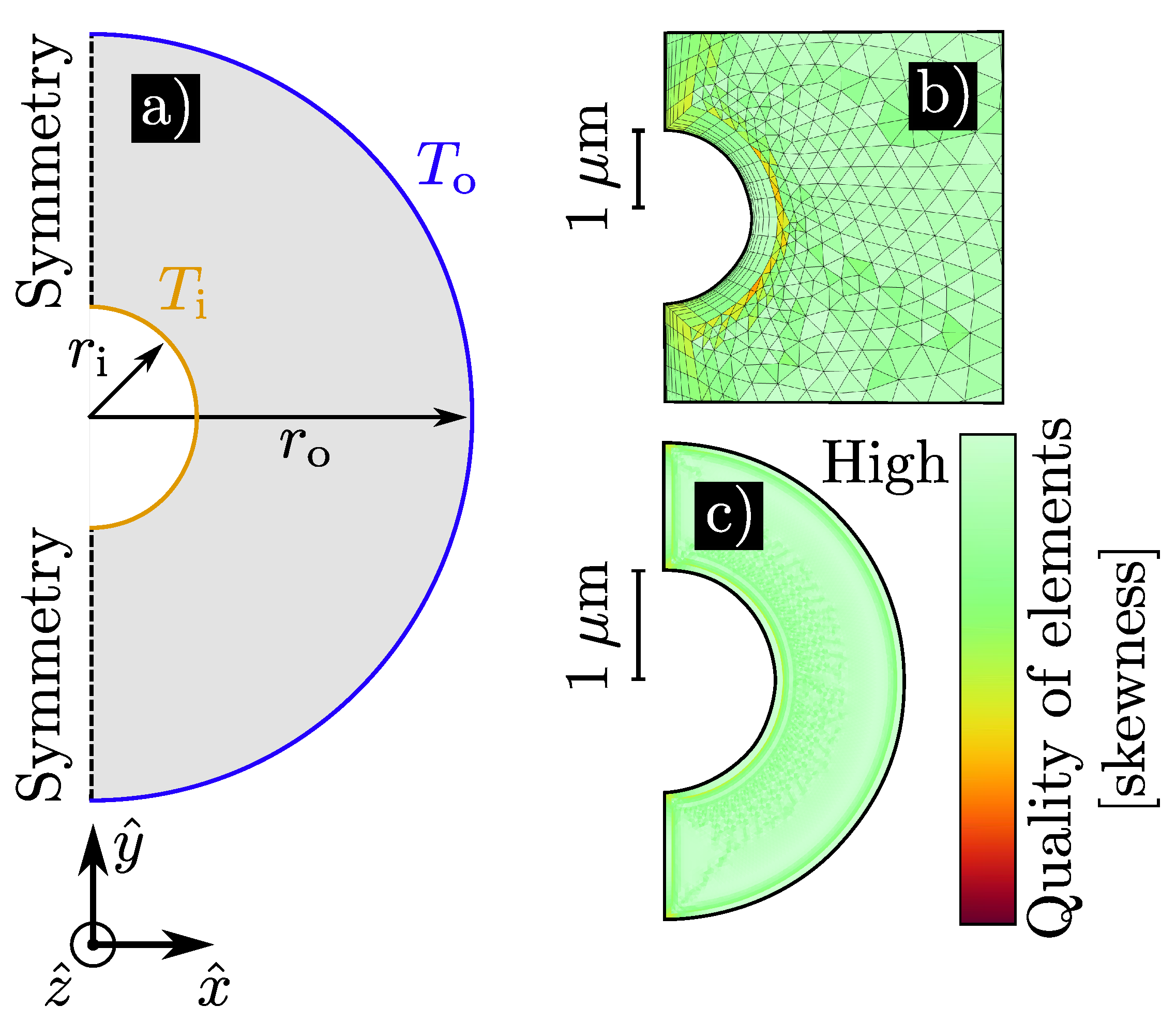
Figure 3.
a) shows the simulated value of for all combinations of parameters done. It is evident that the ratio is close to one for most of the parameter space, but increases once exceeds 1cm–cm. b) Compares some of the results of this work with those predicted by Raithby and Hollands ([1]) as a function of , for 100– and 1, 10 and 100–. Compared to their work, we predict the onset of convection for a substantially smaller .
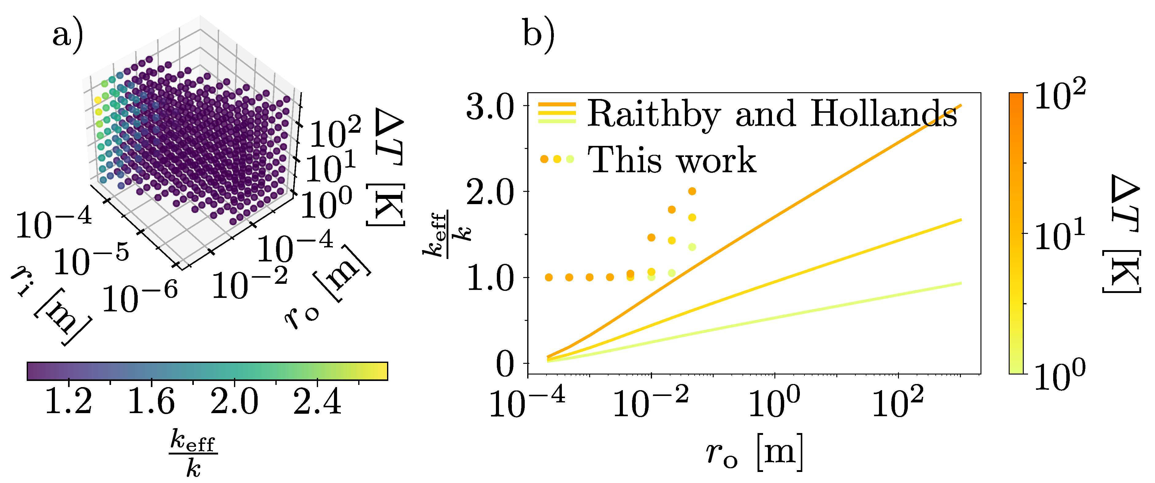
Figure 4.
a) shows velocity streamlines of nine different combinations of and , chosen around the point where starts to increase. As the size of the system increases, the velocity of the air circulation increases. Additionally, the temperature distribution changes from being radial, to a more asymmetrical “plume”. The increased circulation is in turn causing a larger . b) Local temperature plotted as a normalized function of x at for the same nine combinations of and as in a). or all curves. It is clear that as increases, the temperature profile changes. For low values, they are similar to a , which is the solution form for conduction between to cylinders. For larger values of , the temperature profiles develop three distinct regions: Two regions of falling temperatures with increasing distance from the inner cylinder, situated closest to the cylinder walls, and a middle region with a relatively constant temperature.
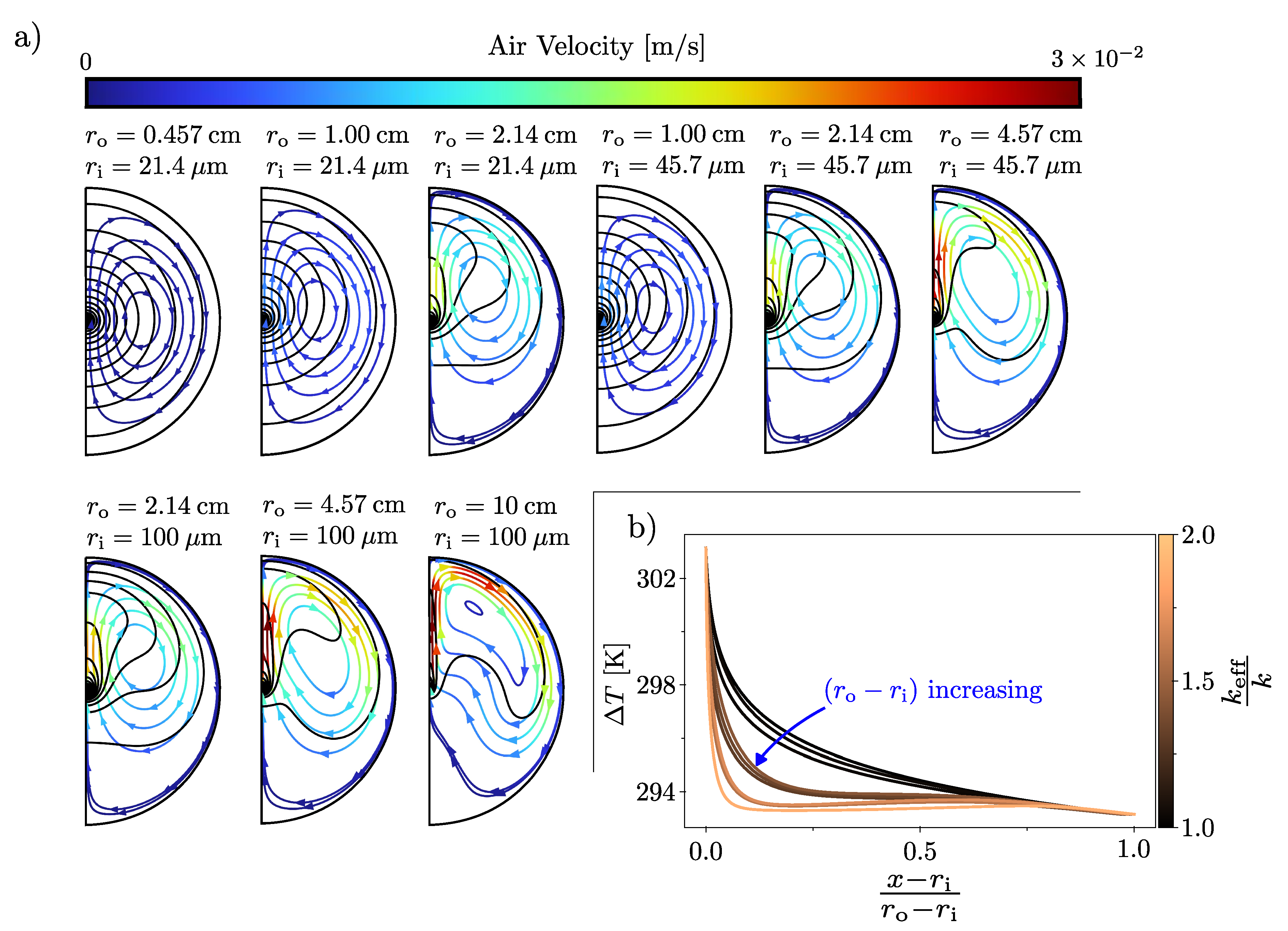
Figure 5.
, as defined in Equation 13 as a function of for a constant in a), and vice versa in b), for three different temperature differences. The analytical solution is based on Equation , assuming .
Figure 5.
, as defined in Equation 13 as a function of for a constant in a), and vice versa in b), for three different temperature differences. The analytical solution is based on Equation , assuming .
Disclaimer/Publisher’s Note: The statements, opinions and data contained in all publications are solely those of the individual author(s) and contributor(s) and not of MDPI and/or the editor(s). MDPI and/or the editor(s) disclaim responsibility for any injury to people or property resulting from any ideas, methods, instructions or products referred to in the content. |
© 2025 by the authors. Licensee MDPI, Basel, Switzerland. This article is an open access article distributed under the terms and conditions of the Creative Commons Attribution (CC BY) license (http://creativecommons.org/licenses/by/4.0/).
Copyright: This open access article is published under a Creative Commons CC BY 4.0 license, which permit the free download, distribution, and reuse, provided that the author and preprint are cited in any reuse.


