
Submitted:
28 October 2025
Posted:
29 October 2025
You are already at the latest version
Abstract
The construction and human operation of reservoirs have made terrestrial hydrological processes increasingly complex, posing challenges to large-scale flood modeling. While many hydrological models have incorporated reservoir operation schemes to improve discharge estimation, the influence of reservoir representation on model parameterization has not been sufficiently evaluated—an issue that fundamentally affects the spatial reliability of distributed modelling. Additionally, the limited availability of reservoir regulation data impedes dam-inclusive flood simulation. To overcome these limitations, this study proposes a synergistic modeling framework for data-scarce dammed basins. It integrates a fully satellite-based reservoir operation scheme into a distributed hydrological model and incorporates reservoir processes into model parameter calibration. The framework’s feasibility was tested using the DRIVE flood model (coupled version named DRIVE-Dam) through a case study in the Nandu River Basin, southern China. Two calibration strategies, with and without dam operations (CWD vs. CWOD), were compared. Results show that reservoir dynamics were effectively reconstructed by combining satellite altimetry with FABDEM topography, successfully supporting the development of the reservoir scheme. Multi-station comparisons across the basin indicate that, while CWD slightly improved streamflow estimation (NSE and KGE > 0.75, similar to CWOD), it enhanced cross-basin peak discharge and flood event duration capture with reduced bias, boosting flood detection probability from 0.54 to 0.60 and reducing false alarms from 0.28 to 0.15. The improvements stem from refined parameterization enabled by a physically complete model structure. In contrast, CWOD leads to subdued flood impulses and prolonged recession due to spurious parameters distorting baseflow and runoff responses, highlighting that neglecting reservoir processes can result in unrealistic parameter estimations and compromised model reliability across space. The proposed methodology provides a technical reference for flood forecasting in dammed watersheds. The findings reveal the enhancement effect of reservoir representation on conventional model parameterization and emphasize the great potential of satellite observations for improving hydrological modeling in data-limited regions.
Keywords:
reservoir operation scheme
; satellite altimetry
; remote sensing
; reservoir dynamics reconstruction
; distributed hydrological model
; parameter calibration
; flood prediction
; DRIVE
1. Introduction
Over recent decades, artificial reservoirs have been constructed worldwide [1,2,3]. While they provide crucial services such as hydropower generation and flood control, reservoirs also fragment river networks [4,5] and alter the timing and distribution of water flows [6,7,8,9,10]. These alterations exacerbate the nonlinearity of water systems and heighten uncertainty in predictions of extreme hydrological events [11,12]. Under the intensifying anthropogenic activities, traditional hydrological models—which are primarily built on natural processes—require essential modifications, such as structure-parameterization, to reconcile discrepancies with realities. This adaptation is a critical step toward improving large-scale hydrological modelling and flood forecasting.
Distributed hydrological models (DHMs) constitute the dominant model family in watershed flood forecasting, requiring parameter calibration for operational application [13,14,15,16,17]. Single-site calibration (SSC) is a basic and widely used method that optimizes model parameters by minimizing discrepancies between simulated and observed flows at a hydrologic station [15,18,19,20,21,22,23,24]. Capitalizing on DHM’s watershed discretization capability, SSC achieves the added benefit of generating optimized flow estimates across upstream multi-areas (subbasins or grid points) using just one gauge [25,26]. Taking this structural advantage, real-time flood forecasting systems at both global and regional scales adopt DHMs as their core engine to provide comprehensive flood information across large domains [17,27,28,29]. Moreover, due to the sparse, unevenly distributed gauges globally, downstream flow records have become the de facto basin-wide hydrological proxies for model calibration and evaluation, leading to the prevalence of SSC [15,30].
However, reservoirs pose challenges to the DHM-SSC framework, potentially leading to estimation errors throughout the basin and reducing the model’s reliability. The parameters to be optimized are typically from DHM’s Land Surface Model component, which generates the hydrological fluxes across the watershed and drives the routing component. This generic structure-parameterization of DHMs is deficient for dammed basins since matching modelled natural flow with observed unnatural (regulated) hydrographs during calibration distorts parameters, inducing not only elevated false alarm rates in downstream flood predictions [17], but also misrepresentation of upstream water conditions, such as surface runoff, infiltration, and baseflow [31]. Alfieri, Bucherie [32] showed that even in operational flood forecasting in well-calibrated catchments, higher uncertainties remain in those where the dam regulation is more prominent. To tackle these challenges, the hydrological community has developed parameter regionalization approaches, which transfer parameters calibrated from small, natural catchments to larger, regulated ones through specific algorithms [33,34,35,36,37]. Yet, as an increasing number of newly constructed reservoirs occupy headwater basins [3,38], these indirect methods will lose advantages, necessitating solutions for direct model calibration.
Integrating reservoir processes into DHMs and including them within the calibration are expected to reduce parameter misestimation. Theoretically, the model’s robustness is affected by both structure and parameter; a more realistic physical structure facilitates better parameterization. Although numerous reservoir operation schemes (modules) have been developed and integrated into DHMs, which (comprehensively reviewed by [39]), they are designed only for better downstream simulation accuracy through improving model structure. Few studies have explored the further influences of reservoir representation on model parameterization. Dang, Chowdhury [31] and Zhong, Zhao [40] incorporated dam regulation into SSC on the Mekong River and China’s Dongjiang basin, respectively, and achieved reduced model error at the downstream calibrated station. Nevertheless, the reliability of the dam-included calibration still lacks comprehensive assessments for the distributed simulation, such as detecting floods at different locations over the basin.
Furthermore, limited data availability constrains reservoir modeling in regulated basins, obstructing the spreading of dam-included DHM calibration among the community. The reservoir operation schemes rely heavily on actual operation data for precise modelling. The layered characteristics of reservoir capacity are the key scheme parameters, need to be calibrated against in-situ storage time series provided by local management authorities [41,42,43,44,45,46,47,48,49]. However, across the globe, strategic water resource policies often restrict data access [1,47,50,51,52,53,54,55,56]. Even GRanD [57], which may be considered as the most comprehensive global reservoir attribute dataset, cannot provide adequate key parameters [58,59]. Moreover, the GRanD includes only about 7,000 large reservoirs globally, while tens of thousands of small- and medium-sized reservoirs [60,61] lack open-access characteristics when incorporated into high-resolution and regional simulations. Thus, developing a reservoir modeling framework independent of ground-based observations and attribute records is essential.
Advances in satellite observation offer opportunities for reservoir modeling in data-scarce regions. Shen, Yamazaki [59] and Hanazaki, Yamazaki [58] utilized monthly remotely sensed surface area data to determine parameters in reservoir schemes. Dong, Yang [47] reconstructed daily reservoir storage by integrating 10-day satellite altimetry with DEM-derived bathymetry, enabling parameter calibration for the reservoir module. These studies have shown the application potential of remote sensing, yet employed it merely as an auxiliary tool for estimating selected parameters, while critical reservoir features such as total capacity were still derived from the GRanD database. A fully satellite-based reservoir operation scheme remains unrealized but would be invaluable for simulating reservoir dynamics in data-unavailable basins. Yassin, Razavi [43] demonstrated the feasibility of using historical storage statistics to define the prior-knowledge-limited scheme parameters. This suggests that a reservoir scheme could be established by reconstructing high-frequency water dynamics through the integration of satellite altimetry and DEM. Notably, existing studies rely on the outdated SRTM DEM for storage estimation [47,51,53,56], whereas new generation, lower-error DEMs, such as the Forest And Buildings removed Copernicus 30m DEM (FABDEM [62]) have yet to be exploited in this context.
This study aims to improve hydrologic model calibration and flood prediction in dam-regulated basins under low-data-availability conditions, focusing on addressing two questions:
- 1)
- How can remote sensing data alone be used to develop a reservoir operation scheme that enhances the accuracy of flow estimation by the DHM at dam sites?
- 2)
- To what extent does incorporating reservoir operations into DHM calibration improve hydrological (flood) estimates across the basin, and what are the associated spatial-temporal effects?
We developed a modeling framework that combines satellite altimetry and DEM data to reconstruct daily reservoir dynamics and establish a reservoir operation scheme, which was incorporated into the DRIVE [17] hydrological model (termed DRIVE-Dam). DRIVE-Dam was tested using two parameter optimization strategies: calibration with dam (CWD) and calibration without dam (CWOD). Multiple basin-internal hydrological stations were utilized to validate the effectiveness of the two calibration strategies. Furthermore, the mechanistic differences in model-internal hydrological response were comparatively analyzed.
2. Study Area
The Nandu River Basin (NRB), Hainan Island’s largest river system, was selected due to its combination of strong reservoir regulation and recurrent flooding characteristics that align with the research aims. This 7,176 km² basin features a 311 km mainstem [63] with a 703 m total elevation gradient (Figure 1). The NRB is characterized by a tropical monsoon climate with mean annual temperatures of 22-26 °C and average precipitation of 1,914 mm. Distinct seasonal precipitation patterns prevail, with >80% of annual rainfall concentrated during the May-October wet season. The July-October typhoon-prone period frequently triggers extreme floods, causing severe socioeconomic impacts [64].
Located in the NRB’s upper reach, Songtao Reservoir functions as the principal hydraulic infrastructure, boasting a 3.345 billion m³ storage capacity[65]. This facility integrates multipurpose operations including flood control, irrigation, municipal water supply, and hydropower generation. Its operational duality involves (1) dry-season prioritization of water allocation for downstream urban-industrial sectors, and (2) wet-season implementation of coordinated flood mitigation through peak shaving and controlled discharge, with strategic impoundment ensuring year-round water security. The dam regulation has significantly modified the hydrological spatiotemporal distribution, compromising flood forecasting and emergency response in the urbanized reaches. During the flood season, the Hainan Meteorological Service must assess flood conditions across the entire basin, not just in the downstream areas, to deliver timely early warnings. This necessitates the development of a dam-included DHM covering the full basin extent. The local water authority’s restriction on real-time sharing of dam operational data with the meteorological agency motivates the use of satellite-based reservoir modeling.
3. Data and Methodology
The proposed modelling framework (as seen in Figure 2) targets a representative DHM calibration situation where only downstream flow observations are available for calibration in a dam-regulated catchment. Reservoir storage time series were first reconstructed using satellite data to establish the reservoir module. A pre-calibration step is designed for the module parameter estimation, after which the DRIVE-Dam can execute the CWD.
3.1. Data Sources
The 1/16° resolution soil, vegetation, and land-cover parameter datasets [66] are employed as the static input for the VIC component of the DRIVE. The DRTR routing component of DRIVE utilizes a 1 km-resolution HydroSHEDS DEM [67] and its derivation of a set of hydrography, which is processed by the DRT algorithm [68,69], including flow direction, flow distance, stream order, slope, and catchment area. Meteorological forcing data include IMERG V07 Final satellite precipitation [70,71], and MERRA-2 wind speed and temperature, linearly resampled to 1/16° resolution matching the VIC spatial mask, at daily temporal intervals. Daily streamflow observations (2001–2017) were obtained from three hydrological stations (Figure 1).
The altimetry data of Songtao Reservoir (2011-2021) were obtained from the multi-source fused and enhanced satellite product published by Shen, Liu [72], including 104 points (average interval: 39.8 days; range: 2–198 days) based on measurements from SARAL (29 days), CryoSat (57 days), and ICESat-2 (18 days) satellite. The 30-m resolution FABDEM was employed to extract reservoir slope topography for deriving water level-area-volume (H-A-V) relationships, as it demonstrates high vertical accuracy globally [62,73]. Official water level and storage records (2015-2021) from the reservoir authority were used to validate the satellite altimetry interpolation and storage variation estimates.
3.2. DRIVE-Dam Hydrological Model Framework
3.2.1. DRIVE Model
The DRIVE distributed hydrological model was chosen as the base for coupling the reservoir scheme and conducting calibration experiments. Developed specifically for flood simulation [17], the DRIVE model integrates the VIC model [74] with advanced land surface flux simulation capability and the DRTR routing model, featuring adaptable river network parameterization across different scales [68,69], thereby enabling flexible multi-scale flood monitoring and forecasting [75]. DRIVE not only serves as the core of the Global Flood Monitoring System (GFMS, with resolutions at 1km and ~12 km, http://flood.umd.edu) but also captures the spatiotemporal evolution of floods at local scales [75,76]. The DRIVE model is well-suited for this study because its VIC component represents a typical land surface model requiring calibration. While Jiang, Wu [77] employed DRIVE for calibration methodology research, their study did not account for reservoir effects. In this study, we adopted a nested-grid configuration, with the VIC operating at a 1/16° resolution and the DRTR routing at a 1 km resolution, extracting baseflow and runoff from the corresponding 1/16° VIC cell.
3.2.2. Development and Coupling of Reservoir Scheme in DRIVE
We developed a parametric reservoir operation scheme to represent the reservoir storage-release process within the DRIVE model explicitly. This scheme builds upon the approach used in LISFLOOD (LISFLOOD Scheme [78]), which vertically partitions the storage capacity into operational zones and estimates the dam release by a piecewise function. This realistic design has established the LISFLOOD Scheme as a prevailing paradigm in reservoir modeling, with numerous derived variants demonstrating effective reproduction of observed reservoir operation patterns [43,47,58,79]. The proposed reservoir scheme aims to estimate the outflow, which first satisfies the mass conservation equations:
where and represent reservoir’s inflows and outflows respectively. P and E represent precipitation and evaporation, respectively, which are vertical fluxes and are already included in the land-surface flux calculations of the VIC model. Equation (2), expressed in finite difference form of equation (1), uses subscripts t and t+1 to denote the current and next model time steps, respectively, in which Vt (water storage of the last step) and Qin are known while and are unknown. The subsequently determined by Equation (3a), which represents the generic operation rule of a reservoir with four operational zones and three characteristic water-level-corresponding storage volumes (the conceptual diagram is shown in Figure 3):
where Vd, Vc, and Vf represent the water storage volumes corresponding to the dead storage level, conservation level, and flood control level, respectively. In this study, we propose to determine Vd, Vc, and Vf via satellite-derived water storage time series (see details in Section 3.3.2) as they are usually not included in publicly available data. Qmin, Qn, and Qf denote the minimum required flow, normal flow, and non-damaging downstream flow, respectively, and are estimated based on simulated inflow. In Equation 3b and 3c, r1 and r2 represent the nonlinear control factors for reservoir outflow when the water storage falls within the two intermediate operation zones. The parameter k determines their response to the storage ratio, needs to be calibrated from 0 to 1. The prior estimation and calibration of these static parameters are detailed in Table S1.
When storage falls below the dead storage level (Vt < Vd), releases are restricted to the minimum required flow (Qmin) to sustain downstream ecological integrity. For water volume between the dead storage and conservation levels (Vd ≤ Vt < Vc), releases prioritize meeting normal downstream water demands (Qn), ensuring efficient water use and maintaining long-term water availability. When storage is between the conservation and flood control levels (Vc ≤ Vt < Vf), releases aim to maintain non-damaging downstream flow (Qf), balancing downstream safety with precautionary flood storage capacity. When storage reaches or exceeds the flood control level (Vt ≥ Vf), the reservoir operation actively increases release to reduce storage and mitigate flood risks rapidly for flood control.
The key changes in our proposed scheme compared to the original LISFLOOD Scheme lies in the modification of storage filling ratio multipliers and when Vd≤Vt<Vf. In the LISFLOOD Scheme, these multipliers are linear functions of Vt. Our tests on multiple reservoirs in China indicated that this leads to an excessively rapid decline in simulated storage volume after the reservoir reaches its maximum storage phase at the end of the wet season. In practical reservoir management in China, outflows during this period are carefully regulated to maintain adequate storage and ensure a continuous water supply throughout the forthcoming dry season. We adjusted the multipliers to nonlinear terms r1 and r2 to address this issue, with detailed explanations provided in Figure S1 in Section S1. The parameter k adjusts the responses of r1 and r2 to the filling ratio, enabling optimal alignment with real variation. In this study, k is set to 0.6 after calibrating.
The proposed reservoir scheme (Equations (2) and (3)) was fully integrated into the DRIVE model (hereafter referred to as DRIVE-Dam), in which each reservoir is simplified as a dam grid cell in the routing scheme, replacing the original river cells, and provides the estimated dam outflow for downstream flow simulation (Figure 3).
3.3. Satellite-Based Reservoir Storage Reconstruction
3.3.1. H-A-V Relationship Extraction from FABDEM
The estimation and calibration of the reservoir module parameters (for Vd, Vn, Vf) require water storage time series. Since in-situ storage could not be directly measured, it needs to be converted from observable water level and surface area data. Previous approaches relied on pairing water levels (H) from satellite altimetry with surface areas (A) from optical imagery using temporally matched remote sensing data - a method often compromised by cloud contamination and data gaps [80,81,82,83]. In this study, we adopted a workflow similar to Dong, Yang [47] for an accurate reconstruction of daily water levels from satellite altimetry data. Then, daily storage volumes (V) were derived using a water elevation-area-storage (H-A-V) relationship, which is defined from high-quality topographic data, circumventing the limitations of the methods based on satellite images.
The H-A-V extraction algorithm adheres to two fundamental principles: (1) topographic consistency, assuming that the H-A relationship below the base water surface in DEM is consistent with that derived from the nearshore slope [84]; and (2) hydraulic connectivity, where topographic features constrain the expansion of the inundated area as the water level incrementally rises in DEM. It first defines the initial water surface of the reservoir in the FABDEM, then iteratively raises the water level. At each rising step, the algorithm identifies adjacent grid cells matching the current surface edge elevation, expanding the inundated area to all neighboring cells at or below this level, thus generating the corresponding H-A pairs. A schematic is shown in Figure 4a, while the delineated reservoir slope inundation zones are presented in Figure 4c. Figure 4a graphically shows the obtained H-A-V curves and their mathematical expression.
Following the H-A pair extraction, the H-A curve was derived using a three-parameter power function. By integrating the H-A function (since surface area represents the derivative of storage volume), we derived the corresponding H-V relationship (Figure 4b). This conversion approach, detailed in Section S2, follows the methodology of Zhong, Zhao [40]. The resulting H-A-V relationships enable the derivation of volume time series (V) from observed water level (H) measurements.
3.3.2. Reconstructing Storage Dynamics
The original fused altimetry product for Songtao Reservoir [72], which contains large irregular temporal gaps, was interpolated to daily resolution using Piecewise Cubic Hermite Interpolation (PCHIP, [85]) after method evaluation. Then, daily water storage variations were derived from daily altimetry using the H-V curve built in Section 3.3.1. A comparison between the two reconstructed hydrological variables and the ground truth is presented in Figure 5. The derived high-temporal-resolution storage dynamics from sparse altimetry data were subsequently applied to calibrate the reservoir module parameters, serving as a viable substitute for missing ground-based observations.
3.4. DRIVE-Dam Calibration and Experimental Setup
With the DRIVE-Dam model, two comparative experiments of the single-site calibration were conducted: CWD (incorporating reservoir operation within DRIVE-Dam) and CWOD (running the original DRIVE). Six optimal parameters of the VIC (Table 1) were calibrated against observed data from the downstream Longtang station. The detailed description of each parameter can be found in Section S3. To relieve the equifinality problem, before the CWD experiment, the reservoir scheme’s parameters were independently pre-calibrated, driven by inflow from CWOD results, rather than simultaneously parameter optimization with the VIC. During the CWD, each update of DRIVE’s parameters adjusted reservoir inflows, which in turn triggered the rescaling of internal storage dynamics within the reservoir module (Figure 6). All calibrations used the Kling-Gupta Efficiency (KGE) as the objective function. The CWD and CWOD were conducted with the Shuffled Complex Evolution-University of Arizona (SCE-UA, [86]) algorithm, while the dam module was pre-calibrated using Particle Swarm Optimization (PSO, [87]). The DRIVE-Dam warm-up period was from 2001 to 2003, followed by a calibration and validation period of 2004-2010 and 2011-2017, respectively. The pre-calibration and validation of the dam module were 2011-2015 and 2016-2021, respectively.
3.5. Performance Metrics and Model Validation
The evaluations were systematically performed on three aspects: (1) the reconstructed reservoir dynamics (Section 4.1), (2) the pre-calibration results of the dam module (Section 4.2), and (3) the comparative performance analysis of flow simulations under DRIVE-Dam’s two calibration strategies (Section 4.3-4.4). The selected long-term skill metrics include the Nash-Sutcliffe Efficiency (NSE), Kling-Gupta Efficiency (KGE), correlation coefficient (CC), percent bias (PBIAS), root mean square error (RMSE), and mean absolute error (MAE), which collectively quantify the agreement between simulated and observed data from multiple perspectives. Notably, model validation was conducted on three gauges rather than being limited to the downstream calibration site, to analyze performance variations caused by the calibration strategies across different locations within the watershed. Additionally, flood events were extracted from both simulated and observed flows to evaluate the flood prediction ability using the probability of detection (POD), false alarm ratio (FAR), and critical success index (CSI). The flood identification threshold is defined as the 95th percentile of long-term streamflow series augmented by half a standard deviation, following the methodology established by Wu, Adler [17] for incorporating minor flood events. A flood event is defined when a day or any consecutive days exceed this threshold, while an exceeding day after a non-exceeding day marks the beginning of a new event. Thus, the flood duration of an event is the sum of its occurrence days. To evaluate the reproduction of flood event magnitudes, the relative peak flow error was assessed. Finally, analyses of runoff and baseflow responses during rainfall events in both dry and wet seasons were conducted to diagnose the mechanism differences between the two calibration strategies. All metrics were calculated as detailed in Section S4.
4. Results
4.1. Validation of Satellite-Derived Reservoir Dynamics
Figure 5 presents validation results comparing reconstructed daily reservoir dynamics against ground observations. Figure 5a shows that the interpolated high-frequency water levels smoothly connect the sparse altimetry points, matching the ground truth. From 2015 to 2021, the CC is 0.95, with a MAE of 1.02 m. Some minor, explainable deviations exist, e.g., peaks and troughs in July 2016 and January 2018 were missed due to the insufficient temporal coverage of the original altimetry data.
Figure 5b validates the storage anomalies derived by applying the H-V relationship (Section 3.3.1) to interpolated altimetry. The results correlate well with observations (CC=0.91, slightly lower than for water levels), with a MAE of 66.99×10⁶ m³ (only ~2% of the reservoir’s total capacity). Note that this robust fitness stems from direct interpolation of non-uniform and sparse multi-source altimetry data (104 points) to a long-term (4,018 days) daily record. The result represents an improvement over the proposed approach from Dong, Yang [47], which relied on linear interpolation of single-frequency (10-day) altimetry products followed by rolling-mean smoothing to obtain daily estimates. The results highlight the flexibility of our approach and demonstrate the feasibility of using low-temporal-frequency satellite data for high-temporal-frequency hydrological modeling. The value of high-quality DEMs for reservoir dynamics reconstruction is also highlighted.
4.2. Pre-Calibration of Reservoir Operation Scheme
As depicted in Figure 6a, the pre-calibrated reservoir module successfully reproduced operation patterns of storage during both calibration (KGE = 0.78) and validation periods (KGE = 0.56), demonstrating the robustness of the reservoir module. Although the CWD result showed degraded storage simulation skills compared to the pre-calibration due to the fixed reservoir parameters and scaled inflow modeling by DRIVE, it derives good model efficiency with a KGE of 0.47 and a CC of 0.58. Figure 6b compares outflow results. The flow magnitudes from both the pre-calibration and CWD were comparable, substantially attenuating flood peaks while increasing dry-season flows relative to the naturally modelled flow (CWOD). This indicates the dam module’s ability to perform critical reservoir functions, and the DRIVE-Dam model is capable of representing reservoir dynamics.
4.3. Performance Evaluation of Streamflow Simulation
4.3.1. Long-Term Modelling Skills
Since this study focuses on an application scenario where only downstream hydrological observations are available for calibration, model performance is evaluated separately for the calibration and validation periods at the calibrated Longtang station. As shown in Table 2, the model demonstrates comparable simulation capabilities regardless of whether reservoirs are incorporated. Although NSE, KGE, and CC values are slightly lower during the validation period, they remain above 0.7, indicating that both calibration strategies ensure the model’s hydrological applicability in this basin.
Although the conventional CWOD strategy can effectively calibrate the model, its simulation skill within the basin lacks robustness due to the neglect of reservoir processes. This is substantiated by Figure 7, which extends the comparison from the downstream station to inner-basin stations. The superior performance of the CWD strategy is demonstrated by all skill metrics at each station. Notably, the significant improvement of CWD occurs at the Santan station (located at the tributary, unaffected by dam regulation), with NSE, KGE, and CC increasing by 0.10, 0.08, and 0.06, respectively. The improved parameterization from explicit reservoir representation boosts model accuracy across both reservoir-influenced and uninfluenced regions. The simulated long-term flow hydrographs are provided in Section S5.
4.3.2. Flow Duration and Seasonality
The analysis of flow duration curves (Figure 8a-c) revealed nuanced differences between CWD and CWOD in simulating flows across various magnitudes. Under low-to-moderate flow conditions (≥50% exceedance probability), CWOD consistently exhibited underestimation, whereas CWD demonstrated closer alignment with observed flows. This indicated that reservoir-aided parameterization improved dry-season flow estimations across watersheds (see hydrographs in Section S5). For the high-flow regime (see inset panels), CWD generated higher simulated extreme flows (top 1%) than CWOD at all stations, showing better agreement with observations. Conversely, within the 1%–6% exceedance range, an inverse contrast is observed, attributed to the tendency of CWOD-optimized parameters to overestimate flood tails.
Streamflow seasonality analysis (Figure 8d–f) showed CWD also better captured the regulatory effects of the reservoir at Longtang station, increasing dry-season flows and reducing wet-season flows. In contrast, CWOD, constrained by the model’s natural process structure, exaggerated seasonal variations, indicating that CWD is a preferable approach for reproducing intra-annual streamflow distribution patterns.
4.4. Model Skills in Capturing Flood Events
4.4.1. Flood Event Detection Capability
Figure 9 demonstrates that CWD outperforms CWOD in detecting flood events. In the basin-wide event evaluation, compared to CWOD, CWD increased the POD by 0.06, reduced the FAR by 0.13, and improved the CSI by 0.09. Importantly, DRIVE-Dam significantly reduced FAR and addressed the issue reported by Wu, Adler [17] that hydrological models without explicit reservoir-dam simulation tend to derive high FAR. Reducing false alarms is critical to avoid ineffective efforts in flood warning and response. As shown in Figure 9, the most significant reduction in FAR (decreasing from 0.33 to 0.12) was achieved at Fucai Station, revealing that reservoir-induced better parameterization enhances the upstream hydrological simulation. This is a positive outcome, as headwater regions are often prone to flash floods but remain challenging for DHMs to simulate accurately.
Additionally, the baseline model outperformed CWOD in terms of POD and CSI, suggesting that even without calibration, the model can effectively detect the occurrence of flood events, relying on relative (rather than absolute) values and statistical metrics derived from the long-term simulations. However, the CWD demonstrated better overall performance compared to the baseline in terms of the CSI metric, attributable to significant improvements in both magnitude (indicated by NSE and KGE scores) and timing (indicated by CC score), as illustrated in Figure 7.
4.4.2. Flood Peak and Duration
Further evaluation of the flood events shows that the CWD yielded more accurate flood peaks than CWOD, as illustrated by the boxplots in Figure 10a. Compared to the baseline model, both calibration strategies significantly improve the accuracy of peak flow. However, CWD exhibits a consistently narrower error distribution than CWOD, indicating greater stability and consistency, with reduced variability in peak flow errors across events. At the Longtang and Santan stations, the median and mean errors under CWD are closer to zero, reflecting a lower level of systematic bias. Furthermore, uncertainty in peak flow errors decreases with increasing catchment area (Fucai<Santan<Longtang). Notably, at the calibrated Longtang station, the exceptionally low errors achieved by the CWD can be attributed to two factors: the use of optimized model parameters and the activation of the reservoir module, which captures the human regulation effect—specifically, the upstream dam’s attenuation of flood peaks being effectively transmitted to the downstream gauge.
Regarding flood event duration, the CWOD exhibits a larger bias than CWD, consistently overestimating flooded time across all stations (Figure 10b). At the two interior hydrologic gauges, the overestimation stems from flawed parameters generated by CWOD, which is led by a relatively flattened hydrograph (see Section 5.2 for details). The two-day overestimation of mean event duration at the downstream Longtang Station reflects both parameterization deficiencies and omitted reservoir operations. In summary, CWD outperforms CWOD in flood event detection, peak flow error, and event duration, while also improving simulation accuracy at both calibrated and inner-basin sites. Thus, CWD is the recommended calibration strategy for flood prediction.
5. Discussion
5.1. Advanced H-A-V Extraction Based on Water Connectivity
The consistent precision of the reconstructed water levels and storage anomalies (Section 4.1) implies that the developed H-A-V curve extraction algorithm, coupled with FABDEM, reliably characterizes the water storage-elevation relationship. The novelty of the algorithm lies in its effective utilization of both hydrological connectivity and terrain slope constraints on water expansion. Conventional curve extraction algorithms typically delineate the maximum reservoir area and then statistically aggregate the water surface area at different elevation levels within this boundary [51,53,88], inherently ignoring hydrological connectivity along the water-land boundary and thus potentially leading to overestimation of water surface area.
We specifically evaluate the accuracy of reconstructed storage anomalies rather than absolute values because the outflow calculation (Equations (1) and (2)) relies on water volume changes rather than absolute storage. In other words, satellite-derived water storage dynamics - even when absolute values are overestimated or underestimated due to unknown subaqueous topography information in DEMs - remain valid for calibrating and validating operation schemes as long as their relative variations are precise. This is critical for reservoir modeling practitioners. We tested three publicly available reservoir bathymetry datasets [89,90,91] on 20 reservoirs across Hainan Island, mainland China, and eastern Africa, and found the provided H-A-V curves unsuitable for water balance calculations. This limitation likely stems from these curves’ focus on approximating complete underwater bathymetry, which compromises their accuracy within the actual water level fluctuation range (active storage room, [92]). Therefore, we suggest that in outflow-oriented reservoir modeling, accurate relative variations are sufficient when bathymetry/storage data are inaccessible.
5.2. Diagnosis of Hydrological Response Mechanism
To elucidate the mechanistic differences between calibration strategies, we conducted two diagnostic analyses on a wet-season heavy rainfall event (Figure 11) and a dry-season minor event (Figure 12). Comparative assessment of hydrological responses reveals that: (1) During wet conditions (Figure 11d–f), CWOD generates exaggerated baseflow but attenuated runoff, resulting in underestimated flood peaks with prolonged recession (Figure 11a–c), whereas CWD better matches observed flood pulses; (2) Under dry conditions, CWD generates lower runoff and higher baseflow than CWOD (Figure 12d–f), leading to sustained higher streamflow (Figure 12a–c). The discrepancies originate from the distinct characteristics of the two calibrated VIC parameter sets (Table 3). The relationship between parameter values and hydrological responses is provided in Section S3.
The underlying reasons for the above phenomena are as follows. During the calibration process in the CWOD, due to the natural physical modeling process, the unregulated flood flows from the model are adjusted to match the dam-attenuated flood peak observations. This mismatch compels the model to reproduce dampened hydrological responses under extreme rainfall, typically manifested as elevated baseflow and suppressed runoff. This may also explain the significant reduction of POD by CWOD compared to the uncalibrated baseline simulations, while CWD led to more balanced pairs of POD and FAR through more reasonable process delineation and parameterization. This response style is propagated across the basin by the lumped parameter setting. In contrast, during the dry season, CWD allows parameter optimization to account for reservoir-induced supplemental water to natural flows, leading to higher streamflow estimates relative to CWOD. These findings support our motivated hypothesis: The absence of reservoir representation in the conventional calibration (CWOD) distorts the parameters, proving that physical structure completeness benefits parameterization.
These findings highlight the critical need to consider watershed-scale effectiveness when conducting model calibration. CWOD is an effective strategy for the calibrated station (NSE = 0.79, KGE = 0.81) even when reservoirs exist upstream, as the lumped parameters inherently integrate and dampen intra-watershed noise. However, its effectiveness is confined to the calibrated site, achieved at the expense of flow fidelity in upstream areas. CWD spatially enhances model efficacy across the basin. For instance, at the Santan station (unaffected by the dam), NSE and KGE increased by 0.10 and 0.08, respectively, compared to CWOD, while the FAR decreased by 0.14. Such improvements are critical for flood forecasting, as human settlements are often distributed along diverse river reaches. Recent research [93] provides evidence that global headwater streamflow exhibits an increasing trend, elevating extreme flood risks—a pressing concern. The CWD strategy should be prioritized for such regions.
5.3. Synergistic Benefits of Enhanced Model Structure and Parameterization
The CWD results underscore that the integrity of the model’s physical structure is a prerequisite for accurate parameterization, as evidenced by the physically sound parameters led by the reservoir scheme’s integration into the DRIVE. Although our experiments were conducted under lumped SSC – a classical hydrological scenario, the proposed methodology holds inherent extensibility. Alternative calibration approaches (e.g., cascade-sequential calibration or multi-site calibration) essentially constitute spatial extensions of this fundamental structure, where a dam positioned upstream of a gauge represents a localized SSC scenario. The CWD enables the model to reproduce reasonable natural hydrological processes in dammed watersheds, serving as a viable alternative to conventional parameter regionalization methods and expanding the model’s applicability for scientific research. Thus, we advocate for a paradigm shift in hydrological modeling from traditional calibration approaches to the CWD strategy.
6. Conclusions
This study proposes a comprehensive DHM modeling framework to address the loss of calibration accuracy in dammed basins, thereby enhancing the temporal and spatial consistency of hydrological processes simulated at the watershed scale. The framework integrates a satellite-based reservoir module into DHM and explicitly incorporates the reservoir storage–release processes into parameter calibration. In the case study, long-term reservoir dynamics—including water level and storage—were reconstructed by integrating multi-source satellite altimetry with DEM-derived topographic data. The reconstructed dynamics were subsequently utilized to develop and pre-calibrate the reservoir operation scheme embedded within the coupled DRIVE-Dam model. Finally, the DRIVE-Dam was calibrated against observed streamflow at the basin outlet. The key findings are as follows:
- High-temporal-resolution (daily) reservoir dynamics can be successfully reconstructed by combining sparse satellite altimetry with DEM-derived topographic information, supporting the development of reservoir operation schemes under data-scarce conditions.
- The explicit representation of reservoir processes contributes positively to DHM calibration, improving the overall accuracy of hydrological estimations across the watershed. In particular, flood modeling performance was notably enhanced, with the POD increasing from 0.54 to 0.60 and the FAR decreasing from 0.28 to 0.15. The improvements originate from the calibration process, with the simulated hydrograph reflecting dam-induced flood peak attenuation in wet seasons and water supplementation in dry seasons, closely matching downstream regulated observations.
- Although the conventional dam-excluded calibration achieves acceptable performance at the basin outlet, it compromises accuracy in upstream regions. The resulting simulations exhibit subdued flood impulses and reduced peak intensities, accompanied by prolonged flood recession and underestimated dry-season discharges. The deterioration stems from spurious parameters resulting from calibrating a reservoir-free model (simulating natural flow) against dam-regulated observations, generating unreasonable baseflow-runoff responses.
The findings highlight the importance of reservoir representation for model parameterization, suggesting that dam regulation should be more deeply integrated into process-based models. The results underscore the significant potential of satellite data to advance hydrological modeling. With the increasing spatial and temporal coverage of Earth observations, such as the Surface Water and Ocean Topography (SWOT) mission [94], this research is expected to offer methodological guidance for flood monitoring and early warning in human-impacted regions.
Supplementary Materials
The following supporting information can be downloaded at website of this paper posted on Preprints.org
Author Contributions
Chaoqun Li: Writing – original manuscript, conceptualization, formal analysis, investigation, methodology development, software development, validation, data collection and analyses, visualization of results. Huan Wu: Writing – review & editing, supervision. Lorenzo Alfieri: Writing – review & editing. Yiwen Mei: Writing – review & editing. Nergui Nanding: Writing – review & editing. Zhijun Huang: Data Curation. Ying Hu: Data Curation. Lei Qu: Data Curation. Xun Li: Funding acquisition.
Funding
This study was supported by the National Natural Science Foundation of China (Grants 42275019 and 42088101), the National Key R&D Program of China (Grant 2024YFC3013302), and the Open Fund Project for Heavy Rain of China Meteorological Administration (Grant BYKJ2024Z10). Partial support was also provided by the Hainan Provincial R&D Program (Grants CXFZ2022J074 and SCSF202203), the Hainan Key Research and Development Project (Grant ZDYF2023SHFZ125), and the International Program Fund for Young Scientific Research Talents in Guangdong Provincial Colleges and Universities.
Data Availability Statement
The altimetry data of Songtao Reservoir are openly available at https://zenodo.org/records/7251283. The FABDEM data are openly available from the University of Bristol (https://data.bris.ac.uk/data/dataset/s5hqmjcdj8yo2ibzi9b4ew3sn). The observed reservoir water level and storage data were collected from the Large Reservoir Hydrological Information Website of the Ministry of Water Resources of China (http://xxfb.mwr.cn/sq_dxsk.html). Streamflow observations from three hydrological stations in the Nandu River Basin were obtained from the Hainan Provincial Meteorological Bureau and are available upon request with permission from the bureau.
Conflicts of Interest
The authors declare that they have no conflict of interest.
References
- Duan, Z.; Bastiaanssen, W. Estimating water volume variations in lakes and reservoirs from four operational satellite altimetry databases and satellite imagery data. Remote. Sens. Environ. 2013, 134, 403–416. [Google Scholar] [CrossRef]
- Chao, B.F.; Wu, Y.H.; Li, Y.S. Impact of Artificial Reservoir Water Impoundment on Global Sea Level. Science 2008, 320, 212–214. [Google Scholar] [CrossRef] [PubMed]
- Spinti, R.A.; Condon, L.E.; Zhang, J. The evolution of dam induced river fragmentation in the United States. Nat. Commun. 2023, 14, 1–9. [Google Scholar] [CrossRef] [PubMed]
- Belletti, B.; de Leaniz, C.G.; Jones, J.; Bizzi, S.; Börger, L.; Segura, G.; Castelletti, A.; van de Bund, W.; Aarestrup, K.; Barry, J.; et al. More than one million barriers fragment Europe’s rivers. Nature 2020, 588, 436–441. [Google Scholar] [CrossRef] [PubMed]
- Grill, G. , et al., Mapping the world’s free-flowing rivers. Nature 2019, 569, 215–221. [Google Scholar] [CrossRef]
- Haddeland, I.; Heinke, J.; Biemans, H.; Eisner, S.; Flörke, M.; Hanasaki, N.; Konzmann, M.; Ludwig, F.; Masaki, Y.; Schewe, J.; et al. Global water resources affected by human interventions and climate change. Proc. Natl. Acad. Sci. 2013, 111, 3251–3256. [Google Scholar] [CrossRef]
- Lettenmaier, D.P.; Milly, P.C.D. Land waters and sea level. Nat. Geosci. 2009, 2, 452–454. [Google Scholar] [CrossRef]
- Hanasaki, N.; Kanae, S.; Oki, T. A reservoir operation scheme for global river routing models. J. Hydrol. 2006, 327, 22–41. [Google Scholar] [CrossRef]
- Zhao, F.; I E Veldkamp, T.; Frieler, K.; Schewe, J.; Ostberg, S.; Willner, S.; Schauberger, B.; Gosling, S.N.; Schmied, H.M.; Portmann, F.T.; et al. The critical role of the routing scheme in simulating peak river discharge in global hydrological models. Environ. Res. Lett. 2017, 12, 075003. [Google Scholar] [CrossRef]
- Poff, N.L.; Allan, J.D.; Bain, M.B.; Karr, J.R.; Prestegaard, K.L.; Richter, B.D.; Sparks, R.E.; Stromberg, J.C. The Natural Flow Regime. Bioscience 1997, 47, 769–784. [Google Scholar] [CrossRef]
- Wang, W.; Li, H.; Leung, L.R.; Yigzaw, W.; Zhao, J.; Lu, H.; Deng, Z.; Demisie, Y.; Blöschl, G. Nonlinear Filtering Effects of Reservoirs on Flood Frequency Curves at the Regional Scale. Water Resour. Res. 2017, 53, 8277–8292. [Google Scholar] [CrossRef]
- Arias, M.E.; Cochrane, T.A.; Kummu, M.; Lauri, H.; Holtgrieve, G.W.; Koponen, J.; Piman, T. Impacts of hydropower and climate change on drivers of ecological productivity of Southeast Asia's most important wetland. Ecol. Model. 2014, 272, 252–263. [Google Scholar] [CrossRef]
- Tsai, W.-P.; Feng, D.; Pan, M.; Beck, H.; Lawson, K.; Yang, Y.; Liu, J.; Shen, C. From calibration to parameter learning: Harnessing the scaling effects of big data in geoscientific modeling. Nat. Commun. 2021, 12, 1–13. [Google Scholar] [CrossRef]
- Chlumsky, R.; Mai, J.; Craig, J.R.; Tolson, B.A. Simultaneous Calibration of Hydrologic Model Structure and Parameters Using a Blended Model. Water Resour. Res. 2021, 57. [Google Scholar] [CrossRef]
- Kupzig, J.; Kupzig, N.; Flörke, M. Regionalization in global hydrological models and its impact on runoff simulations: a case study using WaterGAP3 (v 1.0.0). Geosci. Model Dev. 2024, 17, 6819–6846. [Google Scholar] [CrossRef]
- Gupta, H.V.; Sorooshian, S.; Yapo, P.O. Toward improved calibration of hydrologic models: Multiple and noncommensurable measures of information. Water Resour. Res. 1998, 34, 751–763. [Google Scholar] [CrossRef]
- Wu, H.; Adler, R.F.; Tian, Y.; Huffman, G.J.; Li, H.; Wang, J. Real-time global flood estimation using satellite-based precipitation and a coupled land surface and routing model. Water Resour. Res. 2014, 50, 2693–2717. [Google Scholar] [CrossRef]
- Andersen, J.; Refsgaard, J.C.; Jensen, K.H. Distributed hydrological modelling of the Senegal River Basin — model construction and validation. J. Hydrol. 2001, 247, 200–214. [Google Scholar] [CrossRef]
- K. Ajami, N., et al., Calibration of a semi-distributed hydrologic model for streamflow estimation along a river system. Journal of Hydrology 2004, 298, 112–135. [Google Scholar] [CrossRef]
- Arsenault, R.; Brissette, F.; Martel, J.-L. The hazards of split-sample validation in hydrological model calibration. J. Hydrol. 2018, 566, 346–362. [Google Scholar] [CrossRef]
- Duan, Q.; Sorooshian, S.; Gupta, V.K. Optimal use of the SCE-UA global optimization method for calibrating watershed models. J. Hydrol. 1994, 158, 265–284. [Google Scholar] [CrossRef]
- Shen, H.; Tolson, B.A.; Mai, J. Time to Update the Split-Sample Approach in Hydrological Model Calibration. Water Resour. Res. 2022, 58. [Google Scholar] [CrossRef]
- Sun, R.; Hernández, F.; Liang, X.; Yuan, H. A Calibration Framework for High-Resolution Hydrological Models Using a Multiresolution and Heterogeneous Strategy. Water Resour. Res. 2020, 56. [Google Scholar] [CrossRef]
- Vansteenkiste, T.; Tavakoli, M.; Van Steenbergen, N.; De Smedt, F.; Batelaan, O.; Pereira, F.; Willems, P. Intercomparison of five lumped and distributed models for catchment runoff and extreme flow simulation. J. Hydrol. 2014, 511, 335–349. [Google Scholar] [CrossRef]
- Smith, M.B.; Koren, V.; Zhang, Z.; Zhang, Y.; Reed, S.M.; Cui, Z.; Moreda, F.; Cosgrove, B.A.; Mizukami, N.; Anderson, E.A.; et al. Results of the DMIP 2 Oklahoma experiments. J. Hydrol. 2012, 418-419, 17–48. [Google Scholar] [CrossRef]
- Pokhrel, P.; Gupta, H.V. On the ability to infer spatial catchment variability using streamflow hydrographs. Water Resour. Res. 2011, 47. [Google Scholar] [CrossRef]
- Alfieri, L.; Burek, P.; Dutra, E.; Krzeminski, B.; Muraro, D.; Thielen, J.; Pappenberger, F. GloFAS – global ensemble streamflow forecasting and flood early warning. Hydrol. Earth Syst. Sci. 2013, 17, 1161–1175. [Google Scholar] [CrossRef]
- Alfieri, L.; Libertino, A.; Campo, L.; Dottori, F.; Gabellani, S.; Ghizzoni, T.; Masoero, A.; Rossi, L.; Rudari, R.; Testa, N.; et al. Impact-based flood forecasting in the Greater Horn of Africa. Nat. Hazards Earth Syst. Sci. 2024, 24, 199–224. [Google Scholar] [CrossRef]
- Najafi, H.; Shrestha, P.K.; Rakovec, O.; Apel, H.; Vorogushyn, S.; Kumar, R.; Thober, S.; Merz, B.; Samaniego, L. High-resolution impact-based early warning system for riverine flooding. Nat. Commun. 2024, 15, 1–12. [Google Scholar] [CrossRef]
- Han, J.-C.; Huang, G.-H.; Zhang, H.; Li, Z.; Li, Y.-P. Effects of watershed subdivision level on semi-distributed hydrological simulations: case study of the SLURP model applied to the Xiangxi River watershed, China. Hydrol. Sci. J. 2013, 59, 108–125. [Google Scholar] [CrossRef]
- Dang, T.D.; Chowdhury, A.F.M.K.; Galelli, S. On the representation of water reservoir storage and operations in large-scale hydrological models: implications on model parameterization and climate change impact assessments. Hydrol. Earth Syst. Sci. 2020, 24, 397–416. [Google Scholar] [CrossRef]
- Alfieri, L.; Bucherie, A.; Libertino, A.; Campo, L.; D'Andrea, M.; Ghizzoni, T.; Gabellani, S.; Massabò, M.; Rossi, L.; Rudari, R.; et al. Operational impact-based flood early warning in Lao PDR and Cambodia. Int. J. Disaster Risk Reduct. 2025, 128. [Google Scholar] [CrossRef]
- Gou, J.; Miao, C.; Duan, Q.; Tang, Q.; Di, Z.; Liao, W.; Wu, J.; Zhou, R. Sensitivity Analysis-Based Automatic Parameter Calibration of the VIC Model for Streamflow Simulations Over China. Water Resour. Res. 2020, 56. [Google Scholar] [CrossRef]
- Gou, J.; Miao, C.; Samaniego, L.; Xiao, M.; Wu, J.; Guo, X. CNRD v1.0: A High-Quality Natural Runoff Dataset for Hydrological and Climate Studies in China. Bull. Am. Meteorol. Soc. 2021, 102, E929–E947. [Google Scholar] [CrossRef]
- Miao, C.; Gou, J.; Fu, B.; Tang, Q.; Duan, Q.; Chen, Z.; Lei, H.; Chen, J.; Guo, J.; Borthwick, A.G.; et al. High-quality reconstruction of China’s natural streamflow. Sci. Bull. 2022, 67, 547–556. [Google Scholar] [CrossRef]
- Beck, H.E.; van Dijk, A.I.J.M.; de Roo, A.; Miralles, D.G.; McVicar, T.R.; Schellekens, J.; Bruijnzeel, L.A. Global-scale regionalization of hydrologic model parameters. Water Resour. Res. 2016, 52, 3599–3622. [Google Scholar] [CrossRef]
- Beck, H.E.; Pan, M.; Lin, P.; Seibert, J.; van Dijk, A.I.J.M.; Wood, E.F. Global Fully Distributed Parameter Regionalization Based on Observed Streamflow From 4,229 Headwater Catchments. J. Geophys. Res. Atmos. 2020, 125. [Google Scholar] [CrossRef]
- Song, C.; Fan, C.; Zhu, J.; Wang, J.; Sheng, Y.; Liu, K.; Chen, T.; Zhan, P.; Luo, S.; Yuan, C.; et al. A comprehensive geospatial database of nearly 100 000 reservoirs in China. Earth Syst. Sci. Data 2022, 14, 4017–4034. [Google Scholar] [CrossRef]
- Shrestha, P.K.; Samaniego, L.; Rakovec, O.; Kumar, R.; Mi, C.; Rinke, K.; Thober, S. Toward Improved Simulations of Disruptive Reservoirs in Global Hydrological Modeling. Water Resour. Res. 2024, 60. [Google Scholar] [CrossRef]
- Zhong, R.; Zhao, T.; Chen, X. Hydrological Model Calibration for Dammed Basins Using Satellite Altimetry Information. Water Resour. Res. 2020, 56. [Google Scholar] [CrossRef]
- Wu, Y.; Chen, J. An Operation-Based Scheme for a Multiyear and Multipurpose Reservoir to Enhance Macroscale Hydrologic Models. J. Hydrometeorol. 2012, 13, 270–283. [Google Scholar] [CrossRef]
- Wang, K.; Shi, H.; Chen, J.; Li, T. An improved operation-based reservoir scheme integrated with Variable Infiltration Capacity model for multiyear and multipurpose reservoirs. J. Hydrol. 2019, 571, 365–375. [Google Scholar] [CrossRef]
- Yassin, F.; Razavi, S.; Elshamy, M.; Davison, B.; Sapriza-Azuri, G.; Wheater, H. Representation and improved parameterization of reservoir operation in hydrological and land-surface models. Hydrol. Earth Syst. Sci. 2019, 23, 3735–3764. [Google Scholar] [CrossRef]
- Speckhann, G.A.; Kreibich, H.; Merz, B. Inventory of dams in Germany. Earth Syst. Sci. Data 2021, 13, 731–740. [Google Scholar] [CrossRef]
- Brunner, M.I. , et al., Challenges in modeling and predicting floods and droughts: A review. Wiley Interdisciplinary Reviews-Water 2021, 8, e1520. [Google Scholar] [CrossRef]
- Steyaert, J.C.; Condon, L.E.; Turner, S.W.; Voisin, N. ResOpsUS, a dataset of historical reservoir operations in the contiguous United States. Sci. Data 2022, 9, 1–8. [Google Scholar] [CrossRef]
- Dong, N.; Yang, M.; Wei, J.; Arnault, J.; Laux, P.; Xu, S.; Wang, H.; Yu, Z.; Kunstmann, H. Toward Improved Parameterizations of Reservoir Operation in Ungauged Basins: A Synergistic Framework Coupling Satellite Remote Sensing, Hydrologic Modeling, and Conceptual Operation Schemes. Water Resour. Res. 2023, 59. [Google Scholar] [CrossRef]
- Wu, Y.; Chen, J. An Operation-Based Scheme for a Multiyear and Multipurpose Reservoir to Enhance Macroscale Hydrologic Models. J. Hydrometeorol. 2012, 13, 270–283. [Google Scholar] [CrossRef]
- Shin, S.; Pokhrel, Y.; Miguez-Macho, G. High-Resolution Modeling of Reservoir Release and Storage Dynamics at the Continental Scale. Water Resour. Res. 2019, 55, 787–810. [Google Scholar] [CrossRef]
- Busker, T.; de Roo, A.; Gelati, E.; Schwatke, C.; Adamovic, M.; Bisselink, B.; Pekel, J.-F.; Cottam, A. A global lake and reservoir volume analysis using a surface water dataset and satellite altimetry. Hydrol. Earth Syst. Sci. 2019, 23, 669–690. [Google Scholar] [CrossRef]
- Ali, A.M.; Melsen, L.A.; Teuling, A.J. Inferring reservoir filling strategies under limited-data-availability conditions using hydrological modeling and Earth observations: the case of the Grand Ethiopian Renaissance Dam (GERD). Hydrol. Earth Syst. Sci. 2023, 27, 4057–4086. [Google Scholar] [CrossRef]
- Brunner, M.I.; Naveau, P. Spatial variability in Alpine reservoir regulation: deriving reservoir operations from streamflow using generalized additive models. Hydrol. Earth Syst. Sci. 2023, 27, 673–687. [Google Scholar] [CrossRef]
- Vu, D.T.; Dang, T.D.; Galelli, S.; Hossain, F. Satellite observations reveal 13 years of reservoir filling strategies, operating rules, and hydrological alterations in the Upper Mekong River basin. Hydrol. Earth Syst. Sci. 2022, 26, 2345–2364. [Google Scholar] [CrossRef]
- Giuliani, M.; Herman, J.D. Modeling the behavior of water reservoir operators via eigenbehavior analysis. Adv. Water Resour. 2018, 122, 228–237. [Google Scholar] [CrossRef]
- Li, Y.; Zhao, G.; Allen, G.H.; Gao, H. Diminishing storage returns of reservoir construction. Nat. Commun. 2023, 14, 1–12. [Google Scholar] [CrossRef]
- Bonnema, M.; Sikder, S.; Miao, Y.; Chen, X.; Hossain, F.; Pervin, I.A.; Rahman, S.M.M.; Lee, H. Understanding satellite-based monthly-to-seasonal reservoir outflow estimation as a function of hydrologic controls. Water Resour. Res. 2016, 52, 4095–4115. [Google Scholar] [CrossRef]
- Lehner, B. , et al., Global Reservoir and Dam Database, Version 1 (GRanDv1): Dams, Revision 01. Global Reservoir and Dam Database, Version 1 (GRanDv1): Dams, Revision 01, 2011.
- Hanazaki, R.; Yamazaki, D.; Yoshimura, K. Development of a Reservoir Flood Control Scheme for Global Flood Models. J. Adv. Model. Earth Syst. 2022, 14. [Google Scholar] [CrossRef]
- Shen, Y.; Yamazaki, D.; Pokhrel, Y.; Zhao, G. Improving Global Reservoir Parameterizations by Incorporating Flood Storage Capacity Data and Satellite Observations. Water Resour. Res. 2024, 61. [Google Scholar] [CrossRef]
- Lehner, B.; Beames, P.; Mulligan, M.; Zarfl, C.; De Felice, L.; van Soesbergen, A.; Thieme, M.; de Leaniz, C.G.; Anand, M.; Belletti, B.; et al. The Global Dam Watch database of river barrier and reservoir information for large-scale applications. Sci. Data 2024, 11, 1–18. [Google Scholar] [CrossRef] [PubMed]
- Zhang, A.T.; Gu, V.X. Global Dam Tracker: A database of more than 35,000 dams with location, catchment, and attribute information. Sci. Data 2023, 10, 1–19. [Google Scholar] [CrossRef] [PubMed]
- Hawker, L.; Uhe, P.; Paulo, L.; Sosa, J.; Savage, J.; Sampson, C.; Neal, J. A 30 m global map of elevation with forests and buildings removed. Environ. Res. Lett. 2022, 17, 024016. [Google Scholar] [CrossRef]
- Huang, S. , Water Conservancy Gazetteer of Hainan Province (2001–2010). Hainan Provincial Local Chronicles. 2013, Haikou: Local Chronicles Publishing House. 353.
- Jiang, X.; Ren, F.; Li, Y.; Qiu, W.; Ma, Z.; Cai, Q. Characteristics and Preliminary Causes of Tropical Cyclone Extreme Rainfall Events over Hainan Island. Adv. Atmospheric Sci. 2018, 35, 580–591. [Google Scholar] [CrossRef]
- Lehner, B.; Liermann, C.R.; Revenga, C.; Vorosmarty, C.; Fekete, B.; Crouzet, P.; Döll, P.; Endejan, M.; Frenken, K.; Magome, J.; et al. High-resolution mapping of the world's reservoirs and dams for sustainable river-flow management. Front. Ecol. Environ. 2011, 9, 494–502. [Google Scholar] [CrossRef]
- Schaperow, J.R.; Li, D.; Margulis, S.A.; Lettenmaier, D.P. A near-global, high resolution land surface parameter dataset for the variable infiltration capacity model. Sci. Data 2021, 8, 1–14. [Google Scholar] [CrossRef] [PubMed]
- Lehner, B.; Verdin, K.; Jarvis, A. New Global Hydrography Derived From Spaceborne Elevation Data. Eos Trans. Am. Geophys. Union 2008, 89, 93–94. [Google Scholar] [CrossRef]
- Wu, H.; Kimball, J.S.; Mantua, N.; Stanford, J. Automated upscaling of river networks for macroscale hydrological modeling. Water Resour. Res. 2011, 47. [Google Scholar] [CrossRef]
- Wu, H.; Kimball, J.S.; Li, H.; Huang, M.; Leung, L.R.; Adler, R.F. A new global river network database for macroscale hydrologic modeling. Water Resour. Res. 2012, 48. [Google Scholar] [CrossRef]
- Huffman, G.J. , et al., NASA Global Precipitation Measurement (GPM) Integrated Multi-satellitE Retrievals for GPM (IMERG) Version 07. 2023.
- Huffman, G.J. , et al., Integrated Multi-satellite Retrievals for the Global Precipitation Measurement (GPM) Mission (IMERG), in Satellite Precipitation Measurement: Volume 1, V. Levizzani, et al., Editors. 2020, Springer International Publishing: Cham. p. 343-353.
- Shen, Y.; Liu, D.; Jiang, L.; Nielsen, K.; Yin, J.; Liu, J.; Bauer-Gottwein, P. High-resolution water level and storage variation datasets for 338 reservoirs in China during 2010–2021. Earth Syst. Sci. Data 2022, 14, 5671–5694. [Google Scholar] [CrossRef]
- Wing, O.E.J.; Bates, P.D.; Quinn, N.D.; Savage, J.T.S.; Uhe, P.F.; Cooper, A.; Collings, T.P.; Addor, N.; Lord, N.S.; Hatchard, S.; et al. A 30 m Global Flood Inundation Model for Any Climate Scenario. Water Resour. Res. 2024, 60. [Google Scholar] [CrossRef]
- Liang, X.; Lettenmaier, D.P.; Wood, E.F.; Burges, S.J. A simple hydrologically based model of land surface water and energy fluxes for general circulation models. J. Geophys. Res. Atmos. 1994, 99, 14415–14428. [Google Scholar] [CrossRef]
- Wu, H. , et al., From China’s Heavy Precipitation in 2020 to a “Glocal” Hydrometeorological Solution for Flood Risk Prediction. Advances in Atmospheric Sciences 2021, 38, 1–7. [Google Scholar] [CrossRef]
- Hu, Y.; Wu, H.; Alfieri, L.; Gu, G.; Yilmaz, K.K.; Li, C.; Jiang, L.; Huang, Z.; Chen, W.; Wu, W.; et al. A time-space varying distributed unit hydrograph (TS-DUH) for operational flash flood forecasting using publicly-available datasets. J. Hydrol. 2024, 642. [Google Scholar] [CrossRef]
- Jiang, L.; Wu, H.; Tao, J.; Kimball, J.S.; Alfieri, L.; Chen, X. Satellite-Based Evapotranspiration in Hydrological Model Calibration. Remote. Sens. 2020, 12, 428. [Google Scholar] [CrossRef]
- Zajac, Z.; Revilla-Romero, B.; Salamon, P.; Burek, P.; Hirpa, F.A.; Beck, H. The impact of lake and reservoir parameterization on global streamflow simulation. J. Hydrol. 2017, 548, 552–568. [Google Scholar] [CrossRef] [PubMed]
- Dong, N.; Wei, J.; Yang, M.; Yan, D.; Yang, C.; Gao, H.; Arnault, J.; Laux, P.; Zhang, X.; Liu, Y.; et al. Model Estimates of China's Terrestrial Water Storage Variation Due To Reservoir Operation. Water Resour. Res. 2022, 58. [Google Scholar] [CrossRef]
- Hou, J.; van Dijk, A.I.J.M.; Beck, H.E.; Renzullo, L.J.; Wada, Y. Remotely sensed reservoir water storage dynamics (1984–2015) and the influence of climate variability and management at a global scale. Hydrol. Earth Syst. Sci. 2022, 26, 3785–3803. [Google Scholar] [CrossRef]
- Busker, T.; de Roo, A.; Gelati, E.; Schwatke, C.; Adamovic, M.; Bisselink, B.; Pekel, J.-F.; Cottam, A. A global lake and reservoir volume analysis using a surface water dataset and satellite altimetry. Hydrol. Earth Syst. Sci. 2019, 23, 669–690. [Google Scholar] [CrossRef]
- Li, X.; Long, D.; Huang, Q.; Han, P.; Zhao, F.; Wada, Y. High-temporal-resolution water level and storage change data sets for lakes on the Tibetan Plateau during 2000–2017 using multiple altimetric missions and Landsat-derived lake shoreline positions. Earth Syst. Sci. Data 2019, 11, 1603–1627. [Google Scholar] [CrossRef]
- Gao, H. Satellite remote sensing of large lakes and reservoirs: from elevation and area to storage. WIREs Water 2015, 2, 147–157. [Google Scholar] [CrossRef]
- Liu, K.; Song, C.; Wang, J.; Ke, L.; Zhu, Y.; Zhu, J.; Ma, R.; Luo, Z. Remote Sensing-Based Modeling of the Bathymetry and Water Storage for Channel-Type Reservoirs Worldwide. Water Resour. Res. 2020, 56. [Google Scholar] [CrossRef]
- Fritsch, F.N.; Butland, J. A Method for Constructing Local Monotone Piecewise Cubic Interpolants. SIAM J. Sci. Stat. Comput. 1984, 5, 300–304. [Google Scholar] [CrossRef]
- Duan, Q.; Sorooshian, S.; Gupta, V. Effective and efficient global optimization for conceptual rainfall-runoff models. Water Resour. Res. 1992, 28, 1015–1031. [Google Scholar] [CrossRef]
- Kennedy, J. and R. Eberhart. Particle swarm optimization. in Proceedings of ICNN’95 - International Conference on Neural Networks. 1995. [Google Scholar]
- Biswas, N.K.; Hossain, F.; Bonnema, M.; Lee, H.; Chishtie, F. Towards a global Reservoir Assessment Tool for predicting hydrologic impacts and operating patterns of existing and planned reservoirs. Environ. Model. Softw. 2021, 140. [Google Scholar] [CrossRef]
- Khazaei, B.; Read, L.K.; Casali, M.; Sampson, K.M.; Yates, D.N. GLOBathy, the global lakes bathymetry dataset. Sci. Data 2022, 9, 1–10. [Google Scholar] [CrossRef]
- Yigzaw, W.; Li, H.; Demissie, Y.; Hejazi, M.I.; Leung, L.R.; Voisin, N.; Payn, R. A New Global Storage-Area-Depth Data Set for Modeling Reservoirs in Land Surface and Earth System Models. Water Resour. Res. 2018, 54, 10–372. [Google Scholar] [CrossRef]
- Hao, Z.; Chen, F.; Jia, X.; Cai, X.; Yang, C.; Du, Y.; Ling, F. GRDL: A New Global Reservoir Area-Storage-Depth Data Set Derived Through Deep Learning-Based Bathymetry Reconstruction. Water Resour. Res. 2024, 60. [Google Scholar] [CrossRef]
- Fassoni-Andrade, A.C.; de Paiva, R.C.D.; Fleischmann, A.S. Lake Topography and Active Storage From Satellite Observations of Flood Frequency. Water Resour. Res. 2020, 56. [Google Scholar] [CrossRef]
- Feng, D.; Gleason, C.J. More flow upstream and less flow downstream: The changing form and function of global rivers. Science 2024, 386, 1305–1311. [Google Scholar] [CrossRef] [PubMed]
- Fu, L.; Pavelsky, T.; Cretaux, J.; Morrow, R.; Farrar, J.T.; Vaze, P.; Sengenes, P.; Vinogradova-Shiffer, N.; Sylvestre-Baron, A.; Picot, N.; et al. The Surface Water and Ocean Topography Mission: A Breakthrough in Radar Remote Sensing of the Ocean and Land Surface Water. Geophys. Res. Lett. 2024, 51. [Google Scholar] [CrossRef]
Figure 1.
Nandu River Basin. The Songtao Reservoir regulates the mainstem. The Longtang station (downstream) is used for DRIVE-Dam model calibration and validation, while the Santan (unregulated tributary) and Fucai (dam-upstream) stations assist in performance evaluation.
Figure 1.
Nandu River Basin. The Songtao Reservoir regulates the mainstem. The Longtang station (downstream) is used for DRIVE-Dam model calibration and validation, while the Santan (unregulated tributary) and Fucai (dam-upstream) stations assist in performance evaluation.
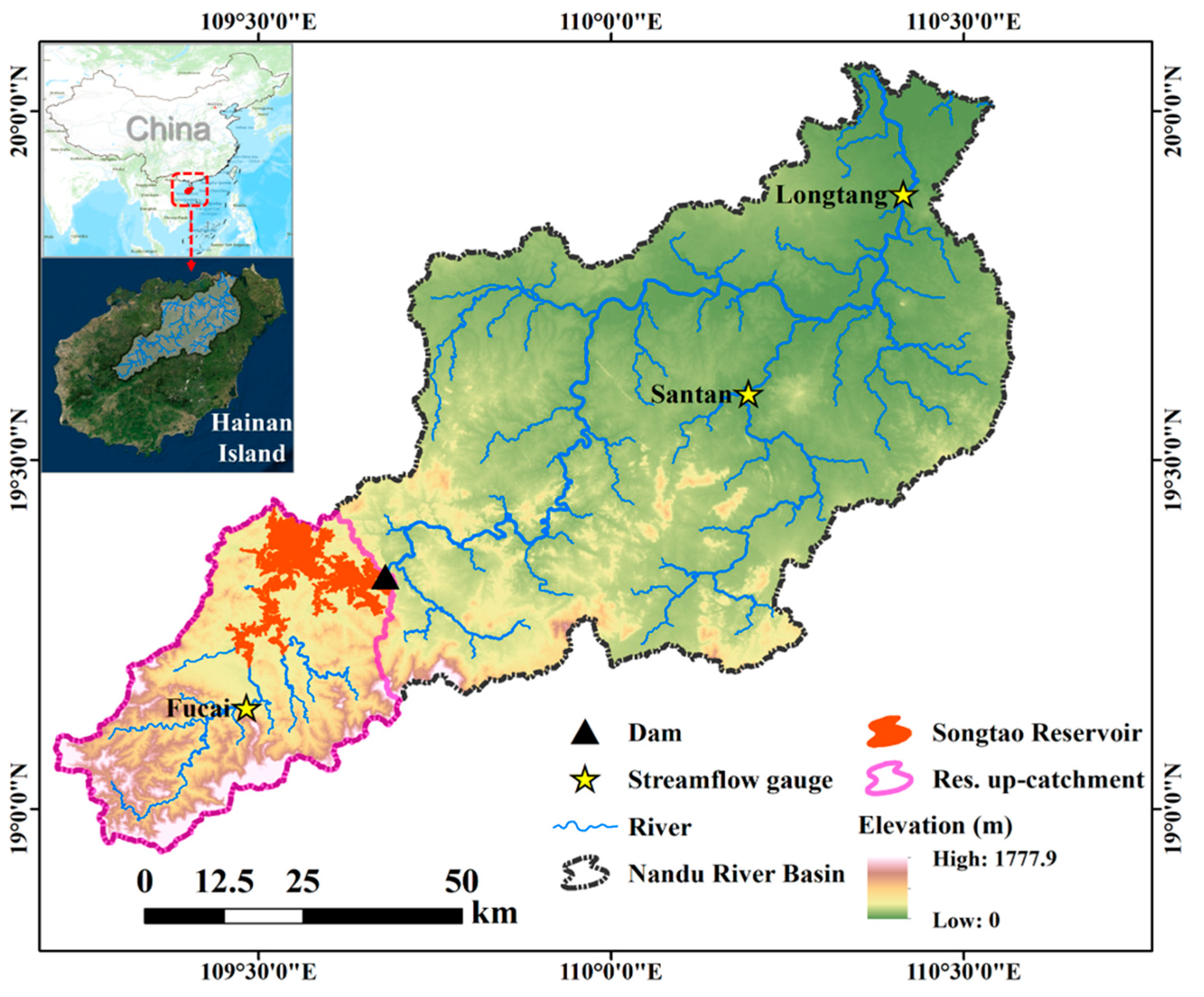
Figure 2.
Flowchart representing the methodology and workflow of this study.
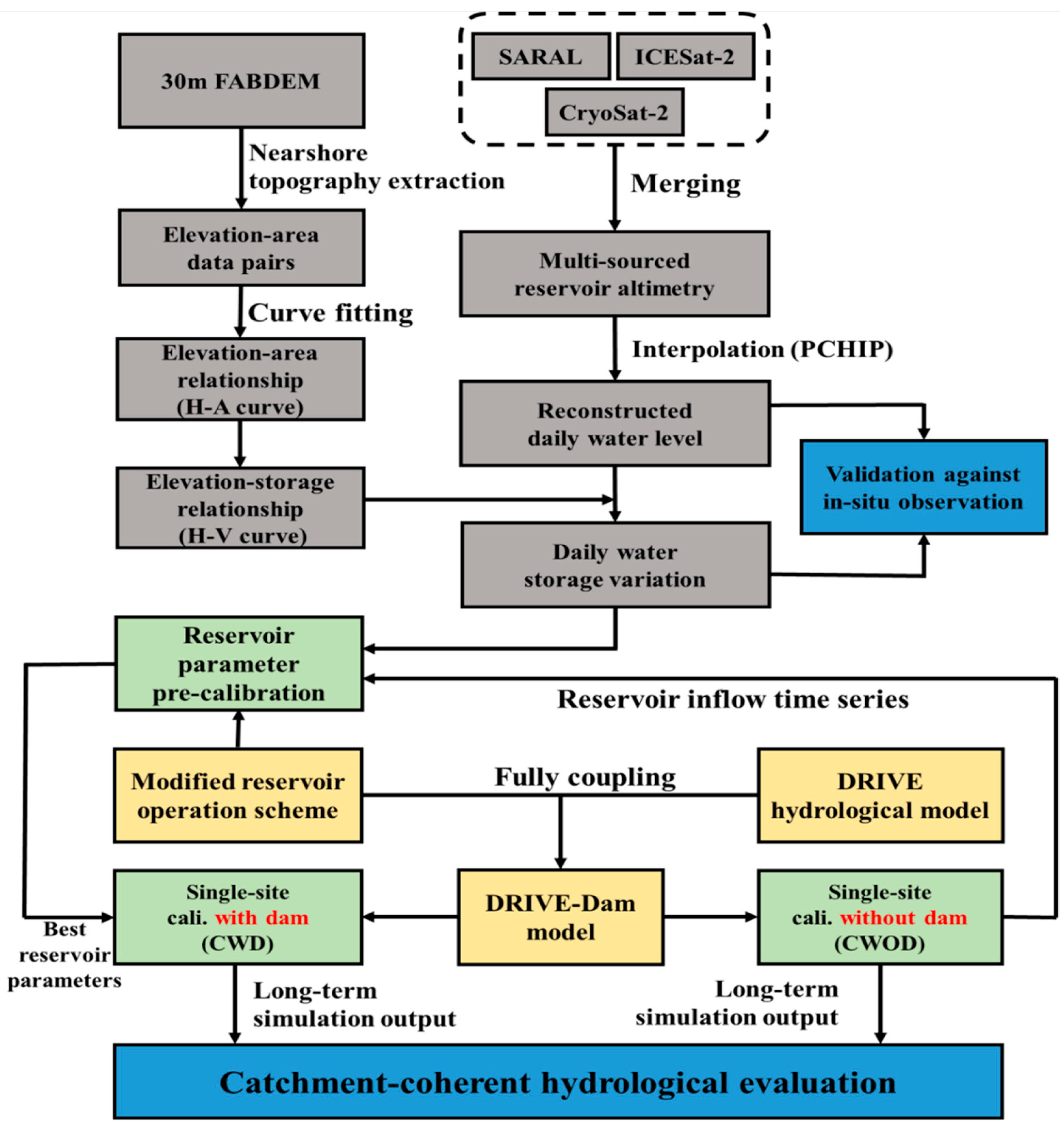
Figure 3.
Schematic of the coupled DRIVE-Dam Model. The upper panels display the original DRIVE model structure, which integrates the VIC and DRTR models. The lower panels illustrate the dam module’s layered operation scheme and grid-cell-based implementation. Vd, Vc, and Vf represent the characteristic water storage parameters corresponding to the dead storage level, conservation level, and flood control level, respectively.
Figure 4.
Water elevation-area-storage (H-A-V) relationship extraction method. (a) The base water surface and shoreline are derived from FABDEM, with incremental inundation based on water connectivity to generate H-A data pairs. (b) A three-parameter power function fits the H-A curve, which is converted to an H-V curve for storage estimation. (c) Visual validation of the base water surface edge (black line) and inundated slopes (colored) from FABDEM against the Landsat image (October 2018, ESRI).
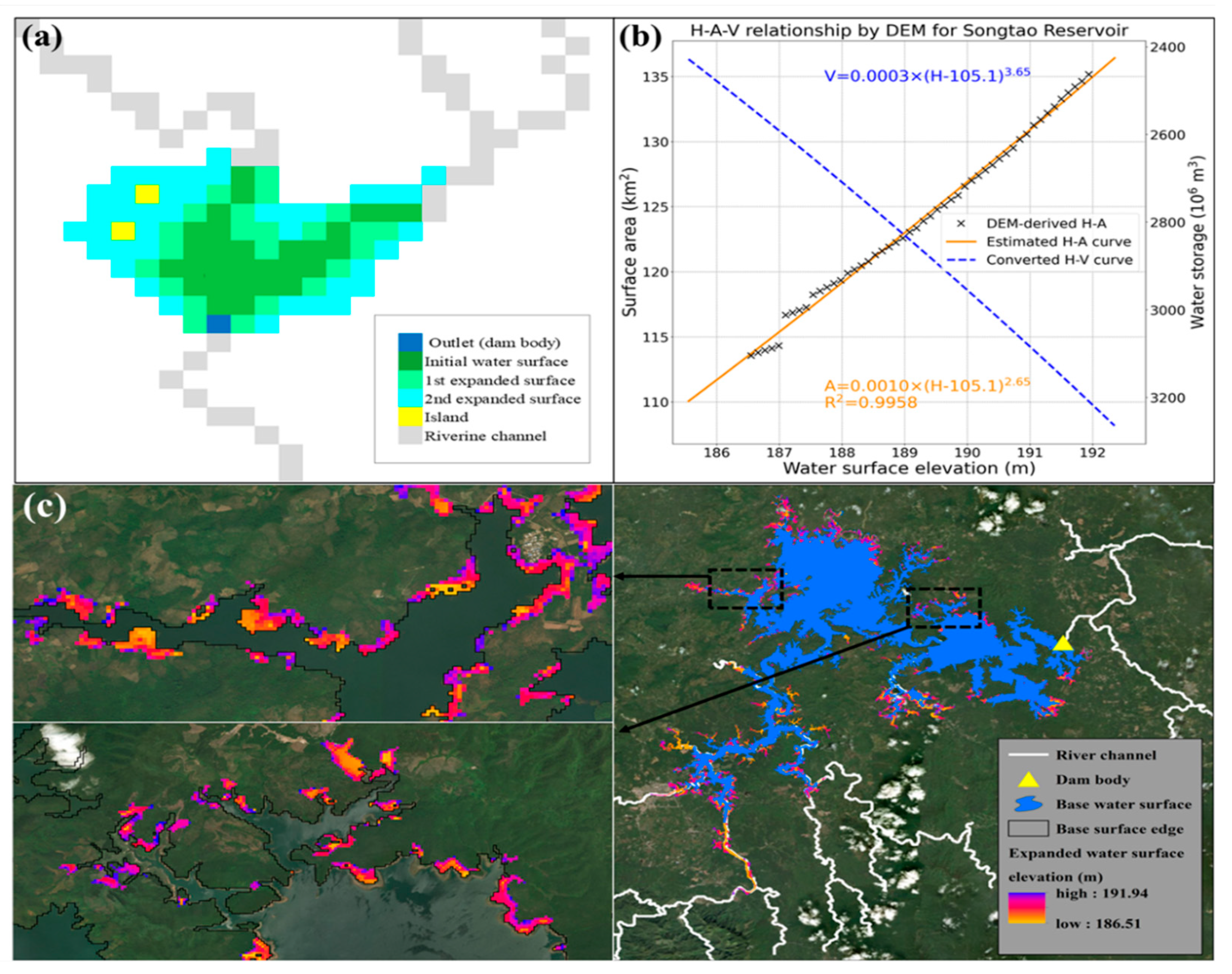
Figure 5.
Validation of satellite-derived reservoir dynamics. (a) Daily water levels interpolated from fused satellite altimetry, compared to in-situ observations. The gray area marks the overlapping period. (b) Remote sensing-derived storage anomalies (orange line, converted from altimetry data using the H-A-V curve) compared to ground observations (green line).
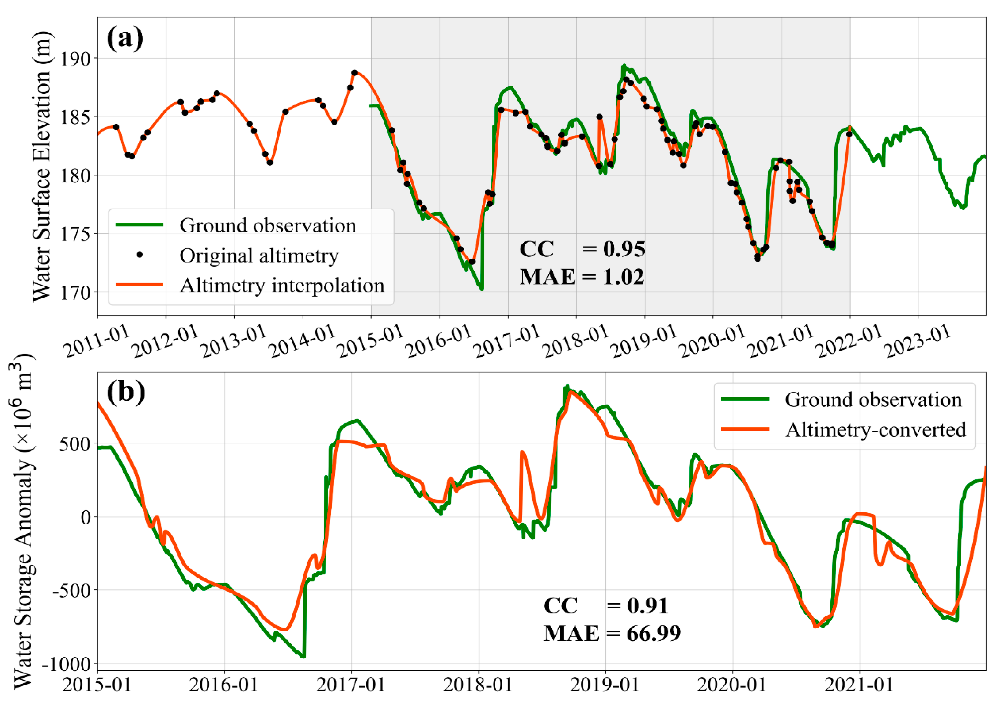
Figure 6.
Validation of reservoir dynamics simulation: Pre-calibration vs. DRIVE-Dam calibration. (a) Water storage comparison: Pre-calibration (2011-2015) of the standalone dam module was performed against satellite-derived storage, forcing by inflow results from the CWOD. The optimized reservoir parameters from pre-calibration were then implemented in CWD. (b) Streamflow comparison at the dam location. For the pre-calibration and CWD, the hydropgraphs are the dam release, whereas the *CWOD denotes the natural flow.
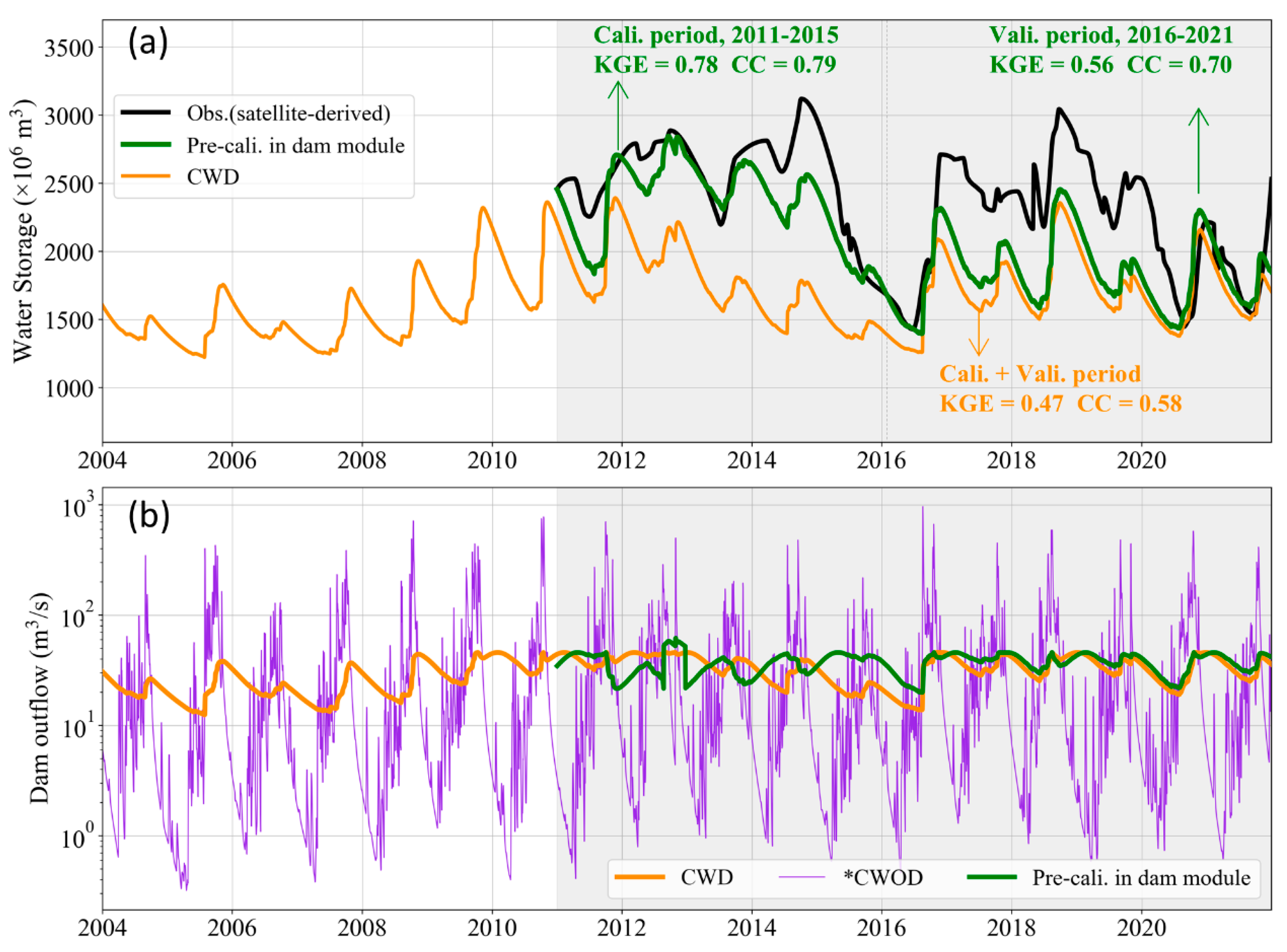
Figure 7.
Comparison of long-term flow performance metrics under two calibration scenarios at each station and the basin scale, covering both calibration (2004-2010) and validation (2011-2017) periods. (a) Nash-Sutcliffe Efficiency (NSE), (b) Kling-Gupta Efficiency (KGE), and (c) Correlation Coefficient (CC). Basin* denotes a weighted aggregation of the three hydrological stations based on their average streamflow.
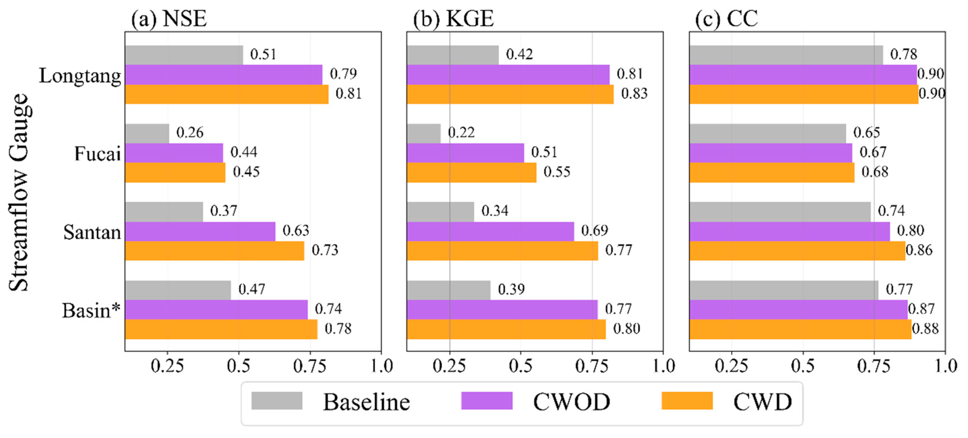
Figure 8.
Evaluation of flow duration and seasonality. (a–c) Flow Duration Curves at each station, showing ranked daily flow comparisons over the entire run period (2004-2017), reflecting model performance across different flow magnitudes. Dual insets within each panel highlight detailed representations of high flow (with 0-1 and 1-6 percentage exceedance, respectively). (d–f) Seasonal variations.
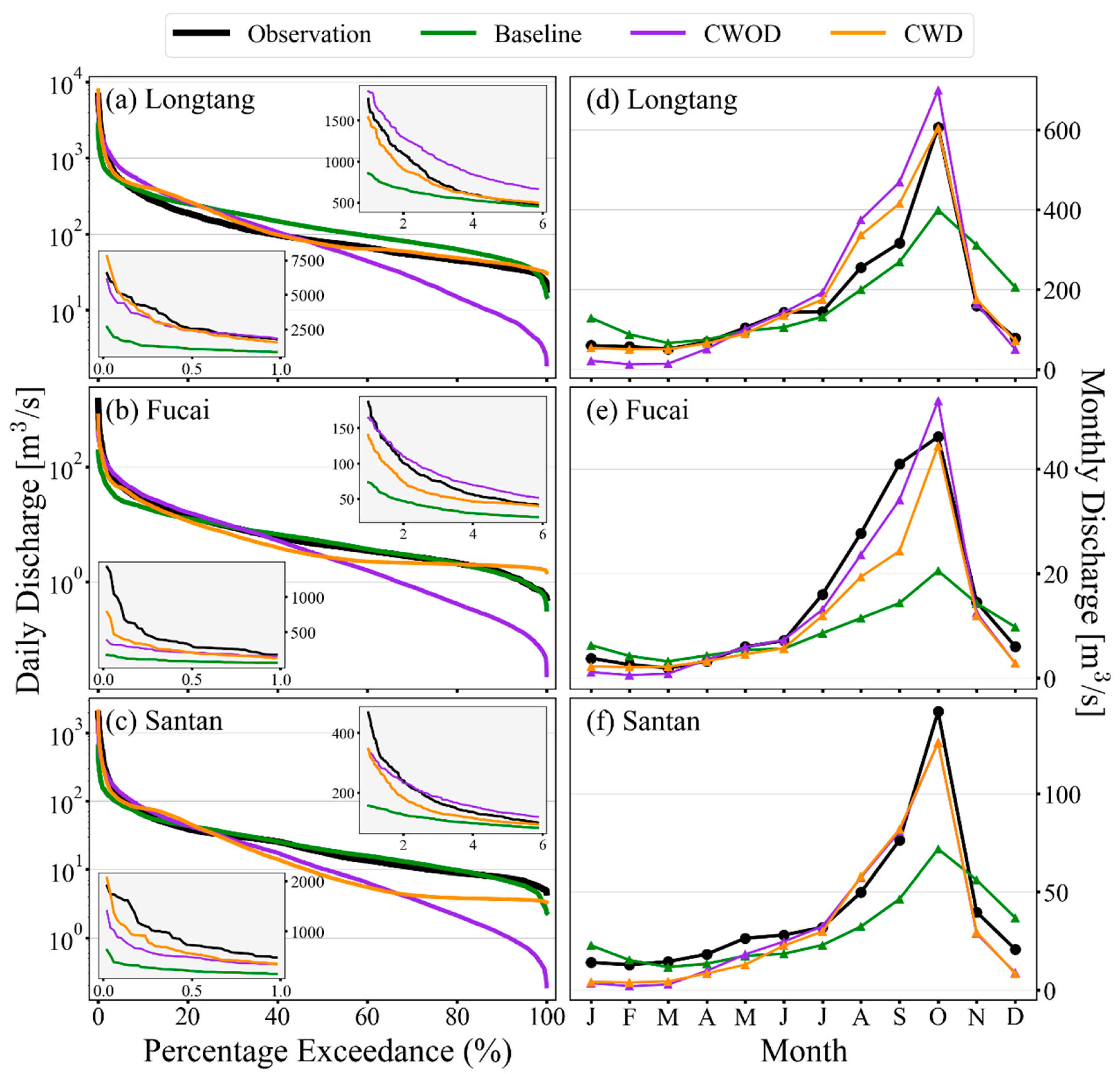
Figure 9.
Evaluation of flood event detection capability: (a) Probability of Detection (POD), (b) False Alarm Ratio (FAR), and (c) Critical Success Index (CSI). The basin* represents the aggregated flood events from all stations.
Figure 9.
Evaluation of flood event detection capability: (a) Probability of Detection (POD), (b) False Alarm Ratio (FAR), and (c) Critical Success Index (CSI). The basin* represents the aggregated flood events from all stations.
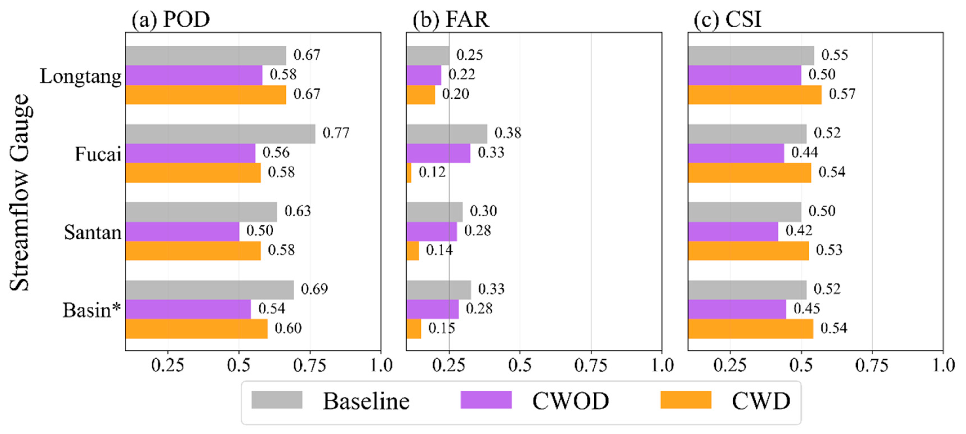
Figure 10.
Comparison of flood peak flow and duration. (a) Boxplots of relative peak flow error (on hit events). (b) Bar plots comparing simulated and observed mean flooding duration.
Figure 10.
Comparison of flood peak flow and duration. (a) Boxplots of relative peak flow error (on hit events). (b) Bar plots comparing simulated and observed mean flooding duration.
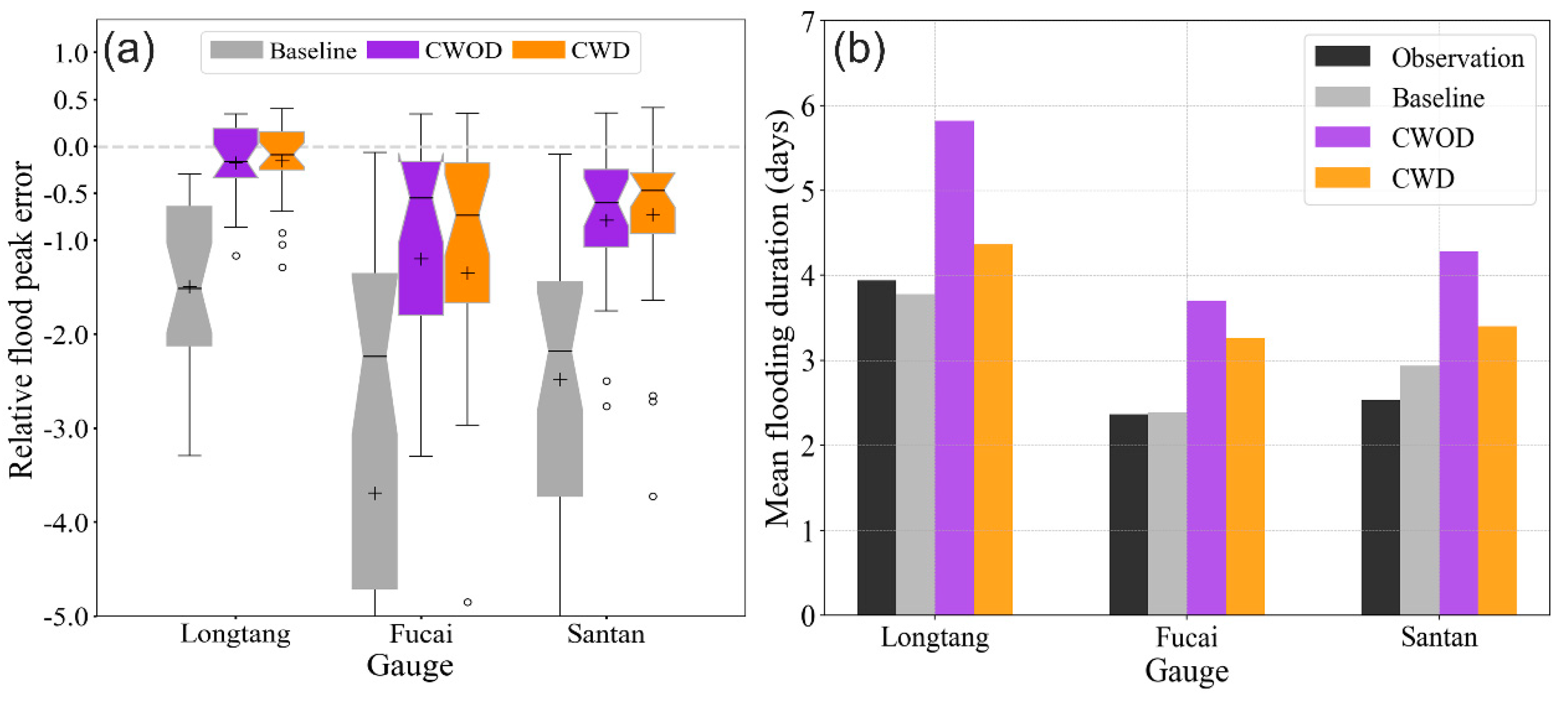
Figure 11.
Hydrological response to an extreme rainfall event in the wet season. (a) Simulated vs observed flows at three stations. (b) Time series of VIC-derived surface runoff and baseflow under different calibration strategies (in the DRIVE-Dam framework).
Figure 11.
Hydrological response to an extreme rainfall event in the wet season. (a) Simulated vs observed flows at three stations. (b) Time series of VIC-derived surface runoff and baseflow under different calibration strategies (in the DRIVE-Dam framework).
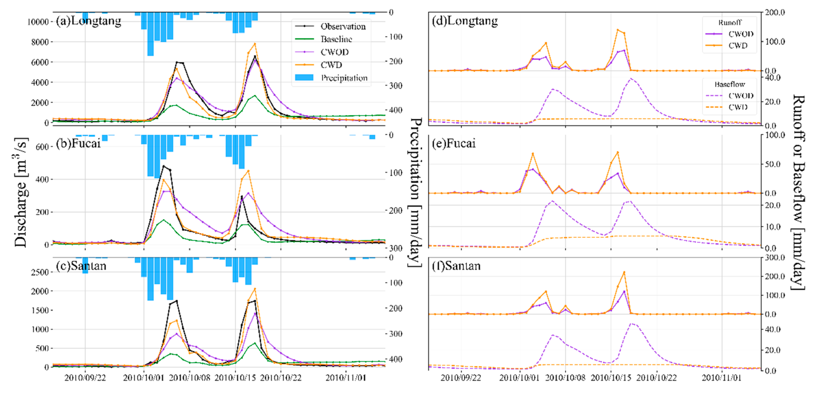
Figure 12.
Same as Figure 11, but for a minor rainfall event during the dry season.
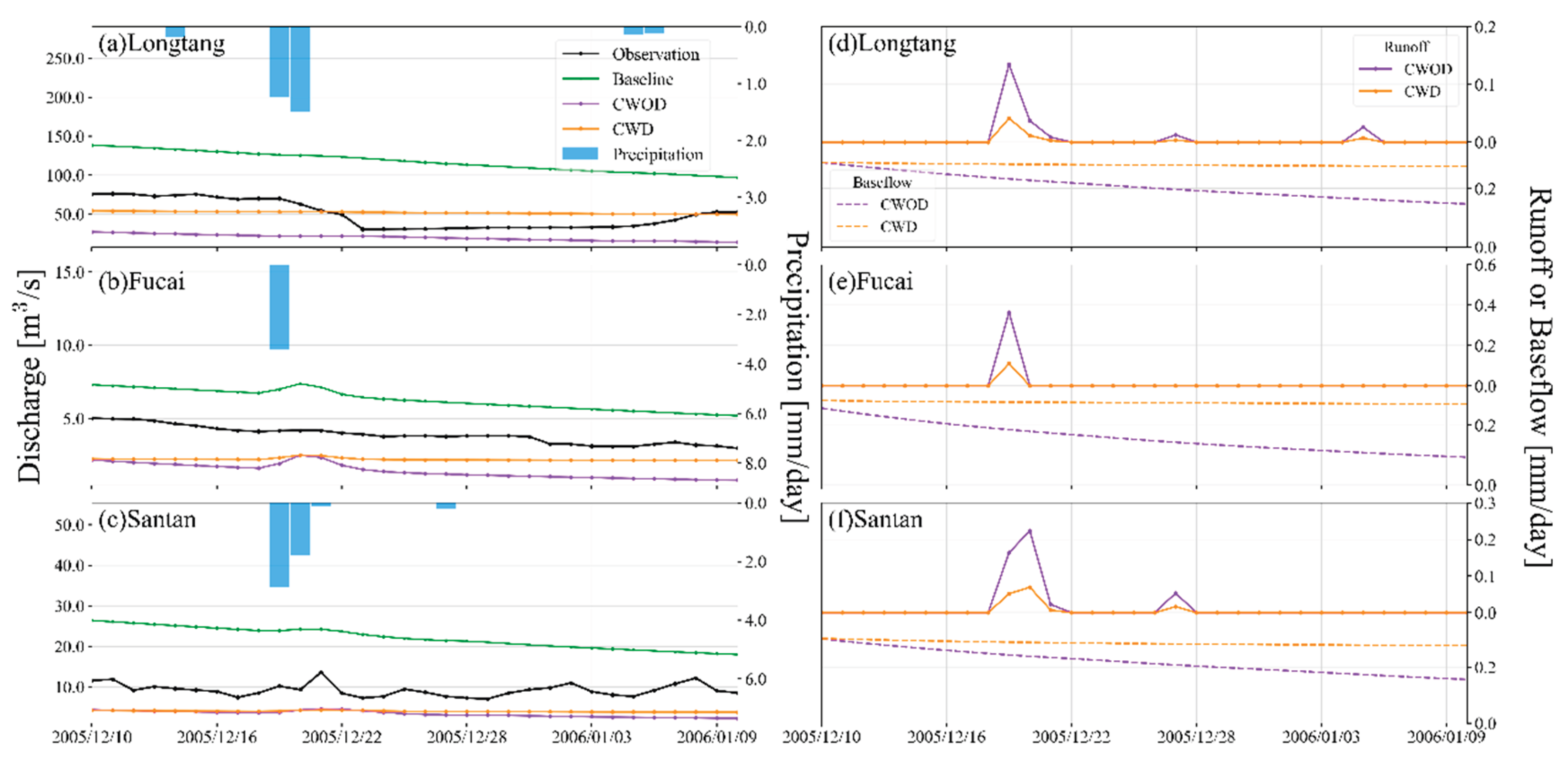

Table 1.
Parameter calibration settings for VIC in the DRIVE-Dam.
| Parameter | Unit | Calibration Range | Default Value in baseline-run |
| Binfilt | N/A | 0.01–1.0 | 0.2 |
| Ds | fraction | 0.01–1.0 | 1 |
| Dsmax | mm/day | 0.01–50.0 | 10 |
| Ws | fraction | 0.01–1.0 | 0.65 |
| d2 | m | 0.30–2.0 | 1.5 |
| d3 | m | 0.30–2.0 | 1.5 |
Table 2.
Streamflow performance during the calibration and validation periods at the calibrated Longtang station.
Table 2.
Streamflow performance during the calibration and validation periods at the calibrated Longtang station.
| Simulation Scenario | NSE | KGE | CC | PBIAS | RMSE | ||||||||||
| Cali. | Vali. | Cali. | Vali. | Cali. | Vali. | Cali. | Vali. | Cali. | Vali. | ||||||
| Baseline | 0.53 | 0.49 | 0.45 | 0.39 | 0.79 | 0.76 | -1.41 | 3.84 | 276.63 | 240.11 | |||||
| CWOD | 0.84 | 0.72 | 0.83 | 0.77 | 0.93 | 0.86 | 12.92 | 11.99 | 160.56 | 175.88 | |||||
| CWD | 0.84 | 0.78 | 0.87 | 0.76 | 0.92 | 0.88 | 7.96 | 9.41 | 162.90 | 157.69 | |||||
Table 3.
Calibrated parameter values of the VIC model in the DRIVE-Dam..
| Scenario | Parameter | |||||
| Binfilt | Ds | Dsmax | Ws | d2 | d3 | |
| CWOD | 0.44 | 0.43 | 31.80 | 0.11 | 1.49 | 0.54 |
| CWD | 0.12 | 0.05 | 5.65 | 0.95 | 0.69 | 1.35 |
Disclaimer/Publisher’s Note: The statements, opinions and data contained in all publications are solely those of the individual author(s) and contributor(s) and not of MDPI and/or the editor(s). MDPI and/or the editor(s) disclaim responsibility for any injury to people or property resulting from any ideas, methods, instructions or products referred to in the content. |
© 2025 by the authors. Licensee MDPI, Basel, Switzerland. This article is an open access article distributed under the terms and conditions of the Creative Commons Attribution (CC BY) license (http://creativecommons.org/licenses/by/4.0/).
Copyright: This open access article is published under a Creative Commons CC BY 4.0 license, which permit the free download, distribution, and reuse, provided that the author and preprint are cited in any reuse.


