
Submitted:
28 October 2025
Posted:
29 October 2025
You are already at the latest version
Abstract
Accurate and efficient simulation of airflows in human airways is critical for advancing the understanding of respiratory physiology, disease diagnostics, and inhalation drug delivery. Traditional computational fluid dynamics (CFD) provides detailed predictions but is often mesh-sensitive and computationally expensive for complex geometries. In this study, we explored the usage of physics-informed neural networks (PINN) to simulate airflows in three geometries with increasing complexity: a duct, a simplified mouth-lung model, and a patient-specific upper airway. Key procedures to implement PINN training and testing were presented, including geometry preparation/scaling, boundary/constraint specification, training diagnostics, nondimensionalization, and inference mapping. Both laminar PINN and SDF-mixing-length PINN were tested. PINN predictions were validated against high-fidelity CFD simulations to assess accuracy, efficiency, and generalization. Results demonstrated that nondimensionalization of the governing equations was essential to ensure training accuracy for respiratory flows at 1 m/s and above. Hessian-matrix-based diagnosis revealed a quick increase in training challenges with flow speed and geometrical complexity. Both the laminar and SDF-mixing-length PINNs achieved comparable accuracy to corresponding CFD predictions in the duct and simplified mouth-lung geometry. However, only the SDF-mixing-length PINN adequately captured flow details unique to respiratory morphology, such as obstruction-induced flow diversion, recirculating flows, and laryngeal jet decay. The results from this study highlight the potential of PINN as a flexible alternative to conventional CFD for modeling respiratory airflows, with adaptability to patient-specific geometries and promising integration with static or real-time imaging (e.g., 4D CT/MRI).
Keywords:
physics-informed neural networks
; PINN
; respiratory flows
; data mapping
; flow constraint
; flow recirculation
; signed distance function
; SDF
1. Introduction
Patient-specific respiratory flow simulation holds clinical promise and vast applications (e.g., lung health diagnostics and inhalation drug delivery); however, it also has bottlenecks posed by meshing, multiscale/complex/dynamic morphology, tidal breathing, and physiological boundary conditions [1,2]. The human respiratory tract spans a vast, branching anatomy from the mouth/nose through the larynx, trachea, and many generations of bronchi, exhibiting marked inter-subject variability in lumen size, curvature, and asymmetry [3]. These geometric features strongly modulate jets (e.g., at the glottis), separations, and secondary flows that govern resistance and deposition [4,5]. Translating segmented CT/CBCT/µCT data into CFD-ready meshes is difficult at scale; despite recent automation efforts, generating boundary-layer-resolving, watertight, high-quality meshes that remain numerically stable across dozens to hundreds of outlets remains labor-intensive [6]. The multiscale morphology variation from mouth (i.e., 20 mm) to alveoli (i.e., 0.3 mm) can demand prohibitive computational resources [7,8,9]. Lack of physiological boundary conditions also hinders respiratory simulations, such as subject-specific inlet waveforms and realistic outlet impedances or flow partitions [10]. Other challenges include validation against in vivo data, which remains scarce for full 3D fields, multiphysics couplings (aerosol transport, heat and moisture exchange) [11], and structural motion and wall compliance that alter airway caliber/resistance and inhaled aerosol deposition [12].
Artificial intelligence (AI) has been used in biofluid simulation as surrogates that approximate CFD solutions (e.g., DeepONets, Fourier Neural Operators) and physics-aware models that embed governing equations into training [13,14,15,16]. Applications in lung health assessment include simulating indoor and airway-like airflows with operator networks and learning parametric maps across breathing conditions [13,14,15]. Physics-informed neural networks (PINNs) encode PDE residuals (e.g., incompressible Navier–Stokes and continuity) into a loss function, enabling mesh-free forward and inverse inference with sparse data [17,18,19]. PINNs have reconstructed flow fields and wall shear in hemodynamics from limited measurements (e.g., 4D-Flow MRI assimilation and pressure/velocity constraints) [20,21,22], and have begun to appear in respiratory settings (e.g., a PINN-based impedance framework for inhalation in symmetric airways) [23]. Algorithmic advances—domain decomposition (XPINNs) for large, 3D, space-time domains; variational/hp-formulations; and self-adaptive loss weighting—improve scalability and robustness [24,25,26]. Still, important limitations persist: gradient and spectral-bias pathologies hinder learning of high-frequency features (boundary layers, jets); training can be slower than conventional CFD per geometry; accuracy deteriorates at higher Reynolds numbers and with complex boundary conditions; and enforcing many outlet constraints over intricate patient-specific topologies remains nontrivial [27,28]. Hybrid strategies (RANS-PINNs with eddy-viscosity closures, data-assimilative PINNs) and decomposition across geometry/time are active remedies but are not yet a turnkey substitute for validated LES/RANS in clinical workflows [24,27,28]. Several architectural/algorithmic variants extend the classical PINN, including NSFnets (Navier-Stokes Flow Nets) that includes velocity–pressure and vorticity–velocity formulations [29], VPINNs (Variational PINNs) that incorporate the variational form of the problem into the loss function to improve training robustness, and Fourier Spectral PINNs that embed high-frequency content and requires shorter training time and lower memory due to the exponential convergence of the spectral basis [30]. Integrating PINN with immersed boundaries has been demonstrated with complex and dynamic walls at high Reynolds numbers [31]. PINNs have also been demonstrated from laminar to (limited) turbulent regimes in canonical benchmarks, but training becomes harder as Reynolds number and geometric complexity increase [29].
Physics-informed neural networks (PINNs) face fundamental dimensional-analysis challenges that stem from the inherent multiscale nature of fluid flow physics and the mathematical structure of the governing equations [17,32]. This entails different challenges in simulating respiratory airflows (more convection-dominated) and cardiovascular flows (more viscosity-dominated) [20,21,22]. Low-density fluids like air (ρ ≈ 1.225 kg/m³) create significantly more training instabilities compared to high-density fluids such as water (ρ ≈ 1000 kg/m³) or blood (ρ ≈ 1060 kg/m³) due to the Reynolds number scaling relationships and the resulting mathematical stiffness of the Navier-Stokes equations [33]. For identical velocity and geometric conditions, the Reynolds number Re = ρVL/μ exhibits dramatically different behavior: airflows typically yield Re values that push the system toward inviscid conditions where viscous terms (1/Re)∇²u become negligible relative to convective terms, creating mathematical stiffness and numerical conditioning issues that manifest as gradient conflicts and convergence failures in neural network training [25,26]. When high velocities are combined with low-viscosity fluids, the resulting high Reynolds numbers create a mathematical regime where the governing equations approach the inviscid Euler limit, causing the solution to exhibit boundary layer physics with thin layers and steep gradients that require resolution across multiple scales simultaneously [34]. This scale separation creates competing optimization objectives in the PINN loss function, where different physics terms have vastly different magnitudes; pressure gradients may be O(10³–10⁶ Pa/m) while velocity magnitudes remain O(1–10 m/s), leading to gradient conflicts during backpropagation where some loss terms overwhelm others [26,35].
The objective of this study is to formulate a PINN-CFD framework for 3D respiratory flow simulations and test it in both simplified and patient-specific airways. Specific aims include:
- (1)
- Test the PINN model in three geometries with increasing complexity.
- (2)
- Evaluate PINN training via the Hessian matrix vs. flow speeds and geometrical complexity.
- (3)
- Nondimensionalize the Navier-Stokes equations to improve training robustness.
- (4)
- Develop an inference module to visualize the PINN results in ANSYS Fluent.
- (5)
- Compare PINN and CFD results of airflows qualitatively and quantitatively.
- (6)
- Compare fidelity between the PINN laminar model and SDF-mixing-length model.
Together, these steps aim to reduce the meshing burden and computational resources while maintaining sufficient fidelity for applications in respiratory health assessment and inhalation therapy.
2. Materials and Methods
2.1. Testing Geometries
The PINN-CFD framework was tested in three geometries with increasing complexity, i.e., a tube, a simplified mouth-lung, and a patient-specific upper airway. The tube has a diameter of 10 mm and a length of 50 mm, similar to the size of the human trachea [36]. Its regular geometry and simple airflow distribution allow us to test the most fundamental PINN functions without the compounding effects of secondary factors. The second test geometry is an elbow-bifurcation configuration representing the human upper airway (Figure 1a). The rationale for selecting this simplified airway is two-fold. First, the 90o elbow has often been used to represent the human oral-throat, with the most notable example being the USP induction port used in pharmaceutical testing [37]. Second, the two-generation bifurcation geometry (Figure 1a) has also been widely used in in vitro testing and computational simulations of respiratory flows. In addition, two of the four outlets (bronchioles) had opposite directions, which was used to test the orientation specification in PINN. The third geometry was a patient-specific upper airway developed by Coley et al. [38] that extended from the mouth opening to the two bronchi (Figure 1b). Fine anatomical details were retained, with dental dips on both sides of the oral cavity, projecting structures of the epiglottis and laryngeal sinuses, and a highly constricted glottis. For all geometries, an inlet velocity of 1 m/s was used, with an equal flow partition among the four outlets in the simplified mouth-lung, and a 60%/40% partition in the patient-specific airway [39].
2.2. CFD Numerical Methods
Steady and incompressible flows were assumed for respiration in this study. ANSYS ICEM CFD and Fluent 21 (Canonsburg, PA) were used to generate the computational mesh and solve airflow dynamics. Considering the relatively low speed at the inlet (i.e., 1 m/s, giving a Re of 667), the laminar flow model was selected. A no-slip condition and rigid walls were assumed for all testing geometries. Flow simulations were considered to have converged when the residuals for both continuity and momentum were reduced by at least five orders of magnitude and exhibited a stable profile. A tetrahedral mesh was generated to resolve each model geometry. Five layers of prism elements were generated in the near-wall region to capture the boundary-layer flows, which have been shown to be essential in resolving boundary layer flows, as well as transport and deposition of both micron and submicron particles [40]. Mesh sensitivity analysis was conducted for the patient-specific airway model by testing six meshes from 1.2–4.2 million, with an approximate increment of 0.6 million. A final mesh size of 3.6 million was observed to generate grid-independent simulation results in the control case (i.e., less than 1% change in velocity magnitude at a sample point in the middle of the trachea).
2.3. PINN
2.3.1. Loss Function
A PINN is a coordinate-based neural field that maps space coordinates (and optional parameters) to continuous fields such as velocity and pressure: (x, y, z, param)→[u, v, w, p)] [17]. The flow physics is embedded via loss-function construction. Training minimizes the composite objective that enforces governing equations and constraints at collocation points:
where L is the loss function that consists of three components: Navier-Stokes equations (NS), boundary conditions (BC), and integral constraints (Constraint). Adaptive weighting was implemented for wBC, which had an initial value of 10 to enforce BCs and reduce the value in the late stage of training following gradient-based weighting [41]. The physics loss is calculated as:
where rc, rx, ry, and rz are the residuals from continuity and the x-, y-, and z-momentum components, respectively. The boundary loss and constraint loss are calculated as:
In the constraint loss, the volume flow rate, , was enforced on each internal slice by integrating the velocity across that slice [17]. The mixing-length turbulence model was used to consider the turbulence effects,
Hereis the magnitude of the strain rate tensor . The mixing length lmix is the distance that a turbulent eddy travels before losing memory of its momentum and is calculated as lmix = min(κ d, rmax Dmax), where κ = 0.419, rmax = 0.09, d is the wall normal distance, and Dmax is the maximum characteristic length. Near walls, lmix ≈ κ d (linear with the wall distance d). The cap (rmax Dmax) prevents lmix from growing indefinitely into the outer or free-stream region where the eddies are bounded by geometry or boundary-layer thickness.
Near-wall treatment was conducted via the signed distance function (SDF), which provided the PINN training a smooth, geometry-aware wall distance and supplied the turbulence closure with the correct near-wall scaling. The SDF has been demonstrated in regularizing the field globally, enforcing gradient consistency, smoothing noise, and improving convergence [42]. In comparison to the boundary loss that defines the morphology (d = 0), the SDF defines how space behaves around the boundary. Considering the viscous term with second derivatives of the velocity, the mixed term scheme was adopted, which introduced auxiliary first derivative fields as unknowns and rewrote the momentum equations using these first-order fields, thus avoiding second derivatives that could cause instability. Compatibility residuals for the first-order gradient field were also enforced, i.e., ui.,j = uj,i.
2.3.2. Architecture
The PINN in this study utilizes a fully connected feedforward architecture implemented within the PhysicsNeMo framework to solve three-dimensional flow problems governed by the Navier-Stokes equations [43]. The network architecture consists of an input layer with three neurons corresponding to spatial coordinates (x, y, z), followed by ten hidden layers, each containing 256 neurons, and culminating in an output layer with four neurons representing the flow field variables (u, v, w, p). This architecture comprises approximately 660,000 trainable parameters, enabling the network to capture complex nonlinear relationships between spatial coordinates and flow variables while maintaining sufficient representational capacity for intricate three-dimensional flow phenomena. Each hidden layer employs standard activation functions (hyperbolic tangent herein) to introduce nonlinearity. The fully connected topology ensures that each neuron receives input from all neurons in the preceding layer, facilitating comprehensive information propagation and enabling the network to learn global spatial dependencies across the computational domain. The physics-informed training methodology constrains the network predictions to satisfy the governing partial differential equations, boundary conditions, and continuity requirements, effectively embedding physical laws into the learning process rather than relying solely on data-driven approaches. This architecture strikes an optimal balance between model complexity and computational efficiency, providing sufficient depth to capture multi-scale flow features while remaining tractable for training on practical computational resources. This makes it particularly suitable for complex three-dimensional fluid dynamics applications where traditional mesh-based methods may be computationally prohibitive.
2.3.3. Nondimensionalization
The mathematical rationale for nondimensionalization in the Navier-Stokes equations extends beyond computational convenience to fundamental solution-space normalization [44]. Nondimensionalization transforms the dimensional equations ∂u/∂t + (u·∇)u = -1/ρ ∇p + ν∇²u into the dimensionless form ∂u/∂t + (u*·∇)u = -∇p + (1/Re)∇²u**, where all variables are scaled by characteristic quantities: u* = u/U, x* = x/L, t* = tU/L, p* = p/(ρU²) [45]. This transformation reveals the underlying physics through dimensionless parameters (Reynolds number, Strouhal number, Froude number) while ensuring that the neural network operates on normalized quantities of order unity, dramatically improving the condition number κ(A) of discretized systems from potentially κ(A) >> 1 in dimensional form to well-conditioned matrices with κ(A) ≈ 1–10 in dimensionless form [46,47].
Nondimensionalization prevents numerical instabilities and maintains balanced loss functions across different physical regimes by ensuring that all terms in the governing equations and boundary conditions are of similar magnitude [29,48]. Without proper scaling, PINN loss functions exhibit Type I gradient conflicts, where different loss terms (PDE residuals, boundary conditions, data fitting) have vastly different gradient magnitudes, and Type II conflicts, where gradients from different terms point in opposing directions, forcing the optimization into inefficient trajectories [49]. The condition number of the Hessian matrix H becomes extremely large (κ(H) > 10⁶) when physical parameters span multiple orders of magnitude, creating elongated valleys in the loss landscape that degrade gradient descent performance [50].
2.3.4. Hessian Matrix and Control Number
The Hessian matrix H and control number κ are important for understanding stiffness and training instability in PINNs. The former is the matrix of second derivatives of the loss function with respect to model parameters θ, H = ∇ 2L(θ), where L includes both data loss and physics loss (residuals from PDE constraints). The condition number κ = λₘₐₓ / λₘᵢₙ quantifies ill-conditioning, with λ being the eigenvalue of the Hessian matrix H. A large value of κ indicates steep curvature, large gradients, and stiff optimization where the network must take tiny steps to stay stable [50]. For 3D Navier–Stokes equations, the λₘ of Hessian typically ranges 105–108 for stiff and ill-conditioned problems. Stiff problems require a small learning rate (≤1e-4) and/or adaptive weights during training, while ill-conditioned problems will diverge unless preconditioned (e.g., NTK scaling, adaptive weighting, or second-order optimizers) [51]. An in-house code was developed to compute the control number κ.
2.4. PINN Training and Visualization
2.4.1. Problem Specification and Training
Figure 2 shows the PINN framework formulated to resolve three-dimensional incompressible flow fields (u, v, w, p). Stereolithography (STL) files were input into the PINN, including inlets, outlets, walls, and interior regions, each subjected to appropriate boundary conditions specifying flow magnitude and direction. To improve numerical stability and facilitate generalization, the governing equations were nondimensionalized using characteristic length and velocity scales (L, V) and fluid properties (ρ, μ). The total loss function comprised the residuals of the governing partial differential equations (PDEs) and boundary conditions, with adaptive weighting factors to ensure balanced optimization. The neural architecture consisted of ten fully connected layers with 256 neurons per layer. Training was conducted in a mesh-free fashion by sampling collocation points within the domain and on the boundaries, minimizing the total loss iteratively until convergence. Diagnostic analyses of the Hessian matrix, including its eigenvalue spectrum (λ) and condition number (κ), were employed to evaluate the stiffness of the optimization problem and to assess the stability and convergence characteristics of the training process (orange block and arrows, Figure 2a). Note that essential steps and potential pitfalls in PINN training were highlighted using dotted color blocks (i.e., nondimensionalization and Hessian diagnostics) and bold letters (i.e., scale, integral constraints, direction, weights), as illustrated in Figure 2a.
2.4.2. Fluent-Based Visualization and Validation
The visualization and validation of the trained PINN model were performed through comparison with computational fluid dynamics (CFD) benchmark data obtained from ANSYS Fluent, as shown in Figure 1b. The PINN-predicted velocity and pressure fields were post-processed and visualized using ParaView and Tecplot, enabling both qualitative and quantitative assessments of the model’s performance. Streamline plots, wall shear stress distributions, and pressure contours were examined to assess the fidelity of the PINN-predicted flow structures relative to the CFD results, particularly in key flow features of respiratory flows. Discrepancies between the PINN and CFD results were also examined using localized error analysis, which provided insights into potential limitations in the training process, such as insufficient boundary condition enforcement or imbalanced loss weighting. This integrated training-visualization-validation workflow aimed to offer a mesh-independent and physics-consistent alternative for flow field prediction and analysis. User-defined modules were developed to export inference points from ANSYS Fluent and map PINN-generated data (VTP and CSV) to ANSYS Fluent. Note that ParaView cannot plot streamlines for PINN-generated mesh-free points. In Figure 2b, mesh-free points were denoted as (x, y, z), while mesh-points were denoted by adding a curly bracket, i.e., {(u, v, w, p)}.
2.4.3. PINN Inference Methodology
The inference mapping capability of PINN (pink block in Figure 2b) enables prediction of flow variables at arbitrary spatial sites without requiring additional computational mesh generation or interpolation schemes. A critical consideration for successful inference mapping is ensuring coordinate system consistency between the training and inference phases. Since the neural network is trained and inferenced in nondimensional systems, the inference coordinates must be provided in the same dimensional units (cm here) as used for training. The trained network outputs nondimensional variables, which are subsequently scaled back to physical dimensions using predetermined scaling factors based on characteristic velocity, length, and pressure scales. Importantly, the nondimensional formulation enhances the generalizability of the trained model, allowing it to handle different Reynolds numbers and geometric scales through appropriate rescaling of the characteristic parameters without requiring retraining of the neural network.
A Fluent-based user-defined function (UDF) was developed to map PINN-predicted flow data at inference points, i.e., (x, y, z)→(u, v, w, p), to ANSYS Fluent computational mesh. A sequential cell-by-cell assignment strategy was implemented, where PINN data points are systematically applied to fluid cells in the order they appear in the mesh structure, which iterates through all fluid threads and cells in the CFD domain, assigning velocity components and pressure values from the PINN dataset to the corresponding Fluent cell variables. This mapping approach hinges on spatial correspondence between PINN inference points and Fluent cell centers, thus overwriting the CFD solution with PINN predictions for comparison purposes. It enables quantitative assessment of PINN accuracy against established CFD benchmarks, enabling rapid evaluation of airflows.
3. Results
3.1. Duct Flow
PINN-predicted airflows in a duct (D: 10 mm, L: 50 mm) are shown in Figure 3a at an inlet velocity of 1 m/s, giving a low Reynolds number of 667, indicating a laminar flow regime. In comparison to corresponding CFD predictions using ANSYS Fluent laminar model in Figure 3b, the PINN captured the pressure and velocity fields in both overall patterns and magnitudes. In the left columns of Figure 3a,b, the elevated pressures at the inlet circumference (shown as two corners in the cross-sectional view) matched well between the PINN and CFD results. This elevation was due to the uniform-velocity inflow impinging on the duct opening. A quantitative comparison of pressure between PINN and CFD is shown in the left column of Figure 3c, which shows relatively low discrepancies overall, while also revealing a descending discrepancy from the inlet to outlet, suggesting a more likely training caveat near the inlet. The development of the flow boundary layer also agreed relatively well between these models, with an asymptotic increase in boundary layer thickness from the inlet to the outlet and a rapid velocity transition in the near wall region (right columns, Figure 3a vs. Figure 3b). However, discrepancies still exist in the near wall region when subtracting PINN velocity field with CFD (right column, Figure 3c), coinciding with the sharp velocity transition within the boundary layer.
3.2. Hessian Matrix-Based Condition Number κ
Note that the PINN result in Figure 3a–c was from the nondimensionalized laminar Navier-Stokes equations. The corresponding duct flow (V = 1 m/s) using the laminar dimensional PINN failed to converge after the same number of training iterations (100,000), showing limited velocity propagations in the inlet and outlet regions. Also note that airflows with an inlet velocity of 3 cm/s converged and showed reasonable pressure and velocity fields, suggesting increasing training challenges with increasing speeds and Reynolds number. To better understand these PINN training challenges, the condition number κ of the Hessian matrix of the loss functions were computed, with Figure 4a showing the mean κ and Figure 4b showing the maximum κ. The magnitude of the maximum κ was three orders of magnitude higher than the mean κ (Figure 4a vs. Figure 4b). Both the maximum and mean κ increased with the inlet velocity, consistent with the observation of training convergence of duct flows at 3 cm/s but non-convergence at 1 m/s. Moreover, the ascending slope of the maximum κ was much steeper than that of the mean κ (Figure 4a vs. Figure 4b).
The mean and maximum condition number κ were also calculated for the simplified mouth-lung geometry and the patient-specific airway at three inlet velocities (3, 30, 300 cm/s). Even steeper ascending slopes were observed with increasing geometrical complexity than with increasing velocity, particularly for the maximum κ. At 300 cm/s, the mean κ was 69.4 for the duct, 1.49×10² for the simplified mouth-lung geometry, and 4.07×10² for the patient-specific airway. By contrast, the maximum κ was 9.79×10² for the duct, 1.05×10⁴ for the simplified mouth-lung geometry, and 2.63×10⁵ for the patient-specific airway, indicating more stringent requirements for training flows in complex geometries.
3.3. Simplified Mouth-Lung Geometry
3.3.1. PINN vs. CFD: Laminar Model
Figure 5a shows the airflows in the simplified mouth-lung geometry at an inlet velocity of 1 m/s (V0 = 1 m/s) using the PINN laminar model, in terms of pressure, velocity, wall shear, streamlines, and coherent structures. The corresponding flow predictions from the ANSYS Fluent laminar model are shown in Figure 5b. Considering the PINN pressure, both the surface and cross-sectional distributions resemble their CFD counterparts in both distribution pattern and magnitude, with slight differences in the 90o elbow, where a low-pressure zone is absent in PINN but present in CFD (black arrow in Figure 5b). The PINN and CFD velocity fields generally resemble each other but also show noticeable differences in the trachea downstream of the 90o elbow. Like normal pressure, the wall shear agrees well between PINN and CFD. Regarding the streamlines, both PINN and CFD captured the recirculation intensity in the upper corner of the elbow (blue arrows in Figure 5a,b); however, the recirculation intensity in PINN appears to be weaker than that in CFD. The vortices predicted by the two models were also compared in terms of the iso-surfaces of the Q-criterion, which show overall similar patterns but nuanced discrepancies in the trachea, where more twisting was predicted in CFD (rightmost panels, Figure 5a vs. Figure 5b).
Quantitative PINN-CFD differences in pressure and velocity are shown in Figure 6a,b, respectively. Again, the pressure in the two selected cross-sections matches between the two models. However, differences were observed at several flow-impingement sites, including the elbow back wall, the carina ridge, and the two bifurcations (black arrows in Figure 6a). The differences in velocity fields are more pronounced, not only in the trachea as visually perceptible in Figure 5, but also in the two main bronchi, and to a less degree, in the four branches.
3.3.2. SDF-Mixing-Length PINN vs. CFD Turbulence Model
To improve the PINN accuracies, the mixing-length turbulence model integrated with the signed distance function (SDF) was implemented in the nondimensionalized Navier-Stokes equations (referred to as SDF-mixing-length PINN henceforth). Figure 7a shows the velocity fields in the two selected cross-sections. It appears that the SDF-mixing-length PINN resolves the flow instabilities in the trachea better than the laminar PINN, that predicted a relatively stable jet along the tracheal back wall, as presented in Figure 5a. Moreover, the velocity field from the SDF-mixing-length PINN agrees more closely with that of the k-ω turbulence model than the laminar model in ANSYS Fluent. The PINN-CFD differences in velocity (third panel in Figure 7a) are most notable in the trachea and main bronchi, similar to those in Figure 6b. However, the magnitude and extent of the differences appear to be smaller in Figure 7a than in Figure 6b. The SDF-mixing-length PINN also better captured the recirculation zone in the upper corner of the elbow, which exhibited similar extent and intensity to that predicted by the ANSYS Fluent k-ω turbulence model (black arrows in Figure 7b).
3.4. Patient-Specific Airway Model
3.4.1. PINN vs. CFD: Laminar Model
The laminar PINN model failed to simulate the flow dynamics (V0 = 1m/s) in the patient-specific airway that had a higher morphological complexity than the other two geometries. As shown in Figure 8, the flow recirculation observed in CFD is absent in laminar PINN, including that in the oral cavity (black arrow) and on both sides of the pharynx (red arrows). The flow fields also differ notably in the two selected cross-sections (second panel in Figure 8), with laminar PINN showing an undeveloped flow pattern in the oral cavity and a prolonged jet flow in the trachea compared with the CFD laminar flow solutions. Hence, the pressure contour and wall shear stress differ significantly between PINN and CFD, particularly in the larynx and trachea (third and fourth panels, Figure 8a vs. Figure 8b).
3.4.2. SDF-Mixing-Length PINN vs. CFD turbulence Model
Figure 9 shows the airflow dynamics (V0 = 1m/s) predicted by the SDF-mixing-length PINN model. Two observations are noteworthy. First, recirculating flows that were absent in the laminar PINN model were captured by the SDF-mixing-length PINN model. These recirculation zones included the teeth-cheek lumen (red solid arrows), the false epiglottis fold (black arrow), and both sides of the pharynx (pink arrows in Figure 9a).
Second, a diverting flow was observed in the oropharynx, as denoted by the hollow arrow in Figure 9a, which coincides with the morphological dip due to the hanging uvula. This uvula-elicited flow diversion indicated that the signed distance function (SDF) adequately responded to the geometrical details, corroborating its role as a spatial regularizer that not only sensed the wall morphology, but also trained the network to enforce the flow field to react to the wall.
Improved similarities were also observed in the velocity, pressure, and wall shear between the SDF-mixing-length PINN and CFD k-ω turbulence model (Figure 9a vs. Figure 9b) compared to those between the laminar PINN and CFD (Figure 8a vs. Figure 8b). These improvements are particularly significant in the throat-trachea region, where both the laryngeal jet and pressure distribution bear a close resemblance to their CFD counterparts (Figure 9a vs. Figure 9b). Quantitative PINN-CFD differences in velocity and pressure are presented in Figure 10a, that confirms their overall similarities and at the same time, discloses subtle velocity differences in the throat region, where large velocity gradients prevail. The wall shear prediction was also improved near the throat, above the carina ridge, and in the main bronchi (green arrows in Figure 9a) than laminar PINN (Figure 8a); however, discrepancies still existed when compared to the CFD k-ω model predictions, for instance, in the mouth roof and middle trachea (brown arrows, Figure 9b). It is also noted that the CFD solutions between the laminar and k-ω turbulence model are very similar (Figure 8b vs. Figure 9b), suggesting a laminar-dominating flow regime consistent with a low inlet Reynolds number of 667.
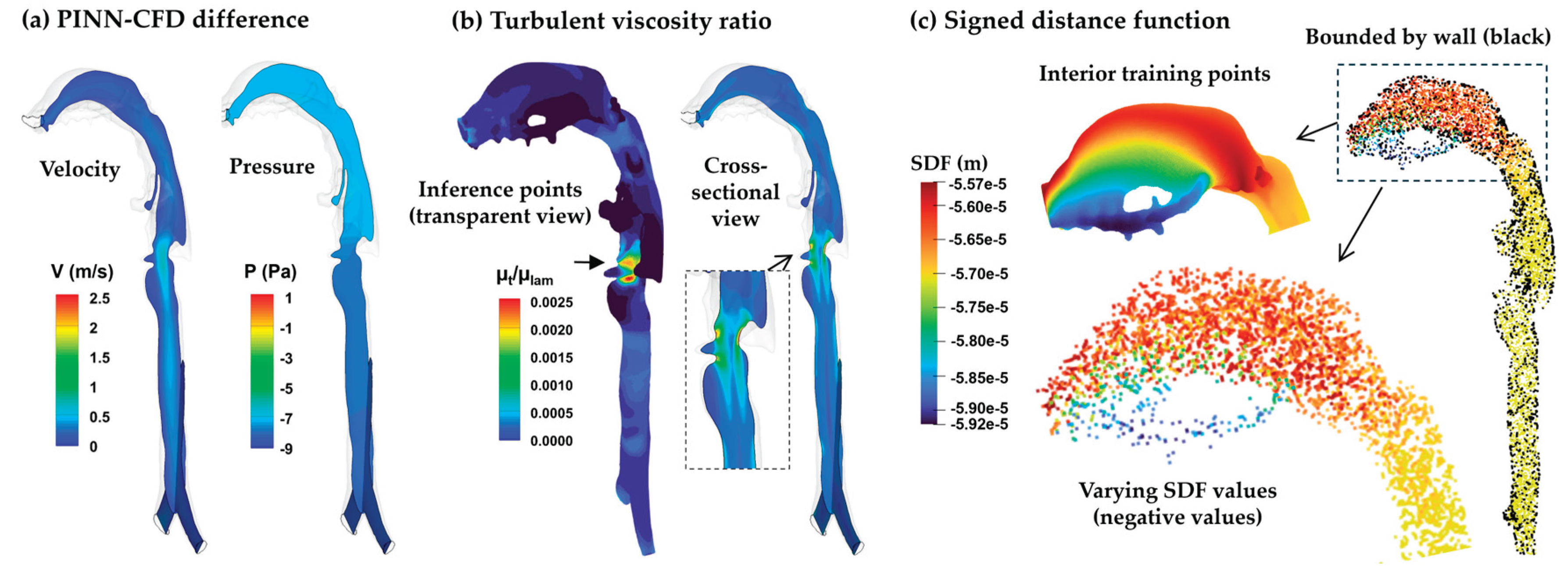
To further evaluate the relative contributions to the improved training accuracy from the SDF and the mixing-length turbulence model, the ratio of the turbulent viscosity over the laminar viscosity (µt/µlam) was recorded on the interior PINN training points (6,000 hereof) and mapped to the inference points from CFD computational mesh (3.6 million), as shown in Figure 10b. Recall that the PINN training points are a point cloud, with no information on point connectivity (i.e., mesh-free), while the inference points are cell centers of the CFD mesh that can be readily mapped back to the mesh with cell connectivity, thus readily allowing cross-section sampling and visualization. The µt/µlam magnitude was low, with the maximum µt/µlam being 0.0025 in the throat region (Figure 10b), indicating negligible effects from the turbulent viscosity. This also implied the PINN improved predictions that were shown in Figure 9a vs. Figure 8a were mainly attributed to the implementation of the SDF, whose values on the PINN interior training points are shown in Figure 10c. Specifically, the closer distance of the training points in the teeth-cheek space (blue color, Figure 10c) may be responsible for resolving the flow dynamics in this constricted region (see streamlines in teeth-cheek space in Figure 9a and the absence of streamlines in Figure 8a).
4. Discussion
4.1. Novelties Compared to Previous Studies
Compared with these prior efforts, this study advanced PINN applications to realistic, patient-specific upper airways that exhibit high morphological and flow complexity under natural breathing (on the order of 1 m/s). Previous studies on PINN primarily focused on canonical benchmarks such as laminar channel and cavity flows (e.g., blood flows), where PINNs achieved good accuracy at low Reynolds numbers but faced convergence issues for high-Re or complex geometries [22]. Unlike laminar-flow PINNs, the present framework integrated nondimensionalized Navier–Stokes equations, internal integral constraints, and SDF-based near-wall treatments to improve stability and fidelity. The results demonstrate that the SDF-mixing-length PINN can capture key flow features, such as obstruction-induced flow diversion, pharyngeal recirculation, and laryngeal jet decay, that were previously unresolved by standard PINN implementations. This represents a step toward scalable, mesh-free PINN modeling of physiological flows comparable in accuracy to CFD solutions while substantially reducing preprocessing overhead.
4.2. Challenges and Best Practices in Implementing and Training PINN
One frequent training problem we have encountered was the “frozen” or “localized” velocity field (i.e., nonzero only near inlet/outlet, zero elsewhere, and discontinuous streamlines), especially at higher flow velocities. This problem could be attributed to various reasons, including gradient imbalance, poor loss scaling, poor boundary enforcement, continuity violation, or numerical stiffness. Note that the loss function is a weighted sum of PDEs, boundary conditions, and other constraints (Eqn. 6), which can easily lead to unbalanced race due to a large discrepancy in convergence rates among different components. Moreover, at high Reynolds numbers, the Navier–Stokes momentum equations become dominated by the convective terms rather than the viscous terms, making the equation more nonlinear and prone to diverge. In this study, two practices were implemented to address the above issues, including nondimensionalization of governing equations, flow constraints in the training domain, and near-wall treatment via the signed distance function, as discussed below in more details.
4.2.1. Nondimensional Governing Equations
The velocity and geometrical complexity were observed to profoundly affect the convergence and accuracy in PINN training, as also observed by Bottou et al. [52]. The underlying mechanisms, however, can be multiple and interconnected. The maximum condition number κmax based on the loss function’s Hessian matrix spanned three orders of magnitude (102–105, Figure 4), which can lead to gradient stiffness and create ill-conditioned optimization problems [53,54]. Jacot et al. [55] demonstrated that poorly scaled parameters lead to near-zero eigenvalues in the loss function and create bias where certain physical parameters are learned slower than others. These problems render normalized, nondimensional PDEs (Navier-Stokes equations) essential to enhance training convergence and accuracy [56]. In this study, the dimensional PINN model was found to work only for well-conditioned problems, for instance, ductal airflows at 3 cm/s; however, even the ductal flows failed when the inlet velocity increased to 1 m/s, presumably due to unbalanced scaling between velocity (1 m/s) and geometry dimension (D = 0.02 m). This study demonstrated that nondimensionalizing the Navier-Stokes equations effectively avoided ill-condition, achieving efficiency convergence and comparable accuracy to CFD solutions, as demonstrated in Figure 3. When enhanced with SDF and the mixing-length turbulence model, the nondimensionalized PINN also exhibits robustness for more complex geometries like the simplified and patient-specific airways (Figure 8 and Figure 9). Advanced strategies also emerged to address these challenges, such as the dimensional analysis-based weighting methods that achieve balanced loss scaling through weights inversely proportional to their loss magnitudes [57], or gradient alignment scores that provide quantitative metrics for diagnosing ill-conditioned problems, with values near zero indicating pathological convergence [58]. Higher-order methods were also proposed to better handle the multi-scale conditioning issues, such as SOAP (Shampoo-based Optimizer) and SIREN (SInusoidal REpresentation Networks), which were reported to achieve 2–10 times accuracy improvements over first-order methods [59]. In this study, we have used the SIREN approach to solve the “frozen” or “localized” velocity field problems with the dimensional PINN but failed. This failure might be due to the inherent ill-conditioning of respiratory flow simulations, which is more likely associated with imbalanced scaling, rather than with high-frequency flow perturbations.
4.2.2. Flow Constraints and GPU Memory Limitation
The other effective approach to mitigate the “frozen” or “localized” velocity field is adding internal slices (integral constraints) to enforce flow continuity. Six slices were used in the patient-specific upper airway along the main flow direction. The integral positions were selected at key anatomical/functional sites such as the oropharynx (flow direction 90o change), the glottis (most constricted), and two bronchi (flow partition), as shown in Figure 1b. At the same time, the integral positions should avoid apparent recirculation zones, where an initial unidirectional flow could slow down the evolution in reversing flow zones. In this study, the PINN model was trained on a NVIDIA GeForce RTX 3090 24G GPU, taking approximately 74 hours to train the patient-specific upper airway model for 200,000 iterations. The number of training points was 4,000 for boundaries (inlet, wall, outlets), 6,000 for the interior, and 9,000 for integral constraints (six slices). Although the total number of points (19,000) appeared not to be excessive, this specification exceeded the training capacity of a 16G GPU. This was because the neural network itself had a baseline of 660,000 trainable parameters, which quickly scaled up the RAM requirement when including flow, boundary, and constraint parameters.
To handle large 3D geometries, domain decomposition has been explored to split space (and/or time) into subdomains, which are trained with local networks and interface conditions [60]. Jagtap et al. [61] proposed cPINN (conservative PINN), which used conservative interfaces on discrete subdomains to enforce flux continuity. Shukla et al. explored Parallel/Distributed PINNs and extended PINNs (XPINNs) that further improved wall-clock performance for large-scale problems [62]. These models are especially relevant for patient-specific airway trees that span many generations and geometrical scales. Note that whole lung simulations are still prohibitively demanding computational resources for conventional CFD due to the enormous mesh requirement to sufficiently resolve the entire airway from mouth to alveoli [8]. In this study, the training time for the patient-specific airway was 74 hours for 200,000 iterations on the NVIDIA GeForce RTX 3090 24G GPU, which was longer than corresponding ANSYS Fluent simulations of 6 hours on a workstation with 4.2+GHz processors and 128 GB RAM.
4.2.3. Near-Wall Treatment via Signed Distance Function (SDF)
The SDF calculated the distance fields in meshfree domains to impose Dirichlet boundary conditions [63]. This geometry-aware trial function was found to be critical to resolve airflows in complex, meshfree geometries like the respiratory tract, as illustrated in Figure 9a vs. Figure 8a. This is reasonable considering that only 6,000 points were used in the interior and 2,000 on the wall, which were three orders of magnitude less than the corresponding ANSYS Fluent computational cells (3.6 million). This low-resolution issue could be further compounded by the imbalanced training rate, where the flow reduced to zero or ‘frozen’ from an over-weighting of the wall loss function. In this study, implementing the SDF not only captured the flows in narrow passages (teeth-check spaces) and the recirculating flows in the two sides of the pharynx, but also captured the flow diversion due to the uvula obstruction (Figure 9a). By contrast, all these flow details were missing in Figure 8a without SDF. As the results in Figure 9a were from a PINN model integrating both the SDF and the mixing-length turbulence model, we confirmed that the improvements were from the SDF implementation, not the mixing-length model, by quantifying the turbulent viscosity on all training points, which were three orders of magnitude lower than the laminar viscosity (Figure 10b). Note that SDF not only enforces exact boundary conditions, but also improves training stability and accuracy near boundaries, with the trial function vanishing on the boundary so the network need not "learn" the boundary condition (BC) [64]. Due to its implicit encoding of the boundary, SDF can better handle complex geometries and enable hybrid schemes and local numerical treatments. For instance, Xiang et al. [64] introduced a hybrid finite-difference and PINN (HFDPINN) that used SDF to prevent stencils from crossing boundaries in complex geometries. Barschkis [65] compared SDF-imposed BC vs. soft/penalty approaches and highlighted tradeoffs and practical implementation notes. A recent review by Plankovskyy et al. [66] recommend SDF, phi-functions, and R-functions as geometry-aware tools for robust PINN boundary handling, with SDF enforcing precise boundary while phi/R functions attaining global multi-body constraints in complex geometries.
4.3. Implications
The success of PINN-based simulation as demonstrated in this study implies potential application of PINN with either static or real-time 4D imaging (e.g., 4D CT or MRI), to efficiently simulate respiratory flows, which could transform diagnosis and management of breathing-related disorders in a patient-specific manner. Traditional CFD-based physiological flow simulations often face challenges of segmentation from low-resolution images, mesh generation for complex geometries, and unavailability of actual boundary (inlet, outlet, and wall) conditions. In contrast, static imaging (CT/MRI) can readily be segmented to render the respiratory geometry as a STL file or a point cloud. Moreover, real-time imaging (4D CT/MRI) can capture dynamic airway deformation and ventilation patterns throughout the breathing cycle, offering rich spatiotemporal data. However, these data alone cannot provide complete flow field information (e.g., local velocity, pressure, or wall shear stress). This is where PINNs can bridge the gap by using partial data from 4D imaging as physics-based constraints to efficiently reconstruct real-time airflow fields. The voxel-wise air–tissue and temporal deformation fields (airway motion) provided by 4D CT/MRI can be used as the internal points and boundary conditions in PINN training. With appropriate loss-weighting, physics-consistent learning can be feasible even from sparse or noisy data [67].
A unified PINN-CFD-4DCT/MRI model has many advantages. It is mesh-free, can naturally handle deforming boundaries, integrates image-derived constraints, and can potentially operate in real-time (after training). Its applications can be many and clinically significant. In patient-specific airway diagnostics, it can assess airflow obstruction, resistance, and regional ventilation. and detect local abnormalities (e.g., stenosis, collapse) in conditions such as COPD or asthma; in virtual surgery or stent planning, it can simulate airflow before and after nasal or tracheal reconstruction, while in drug delivery, it can account for imaging-based anatomical changes during inhalation and recommend the optimal delivery protocol considering device-, formulation-, and patient-related variables. Such potential has been evidenced by a recent surge of research efforts aiming to integrate PINN/CFD with 4DCT/MRI [68,69,70].
4.4. Limitations and Future Directions
Although the present study demonstrates the feasibility of using PINN for three-dimensional respiratory flows, several limitations remain: low training efficiency, limited scalability, laminar-dominant assumptions, steady inhalation, rigid walls, and flow-only modeling. First, the training efficiency remains low, requiring around 74 hours vs. 6 hours using CFD simulations for steady flows in the patient-specific airway. Second, GPU requirements are still high (24G GPU for the patient-specific airway), limiting the scalability. Future developments should integrate domain-decomposition frameworks such as cPINNs and XPINNs, which distribute training across subdomains [61,62]. Parallelization, adaptive sampling, and operator-based learning (e.g., DeepONets, Fourier Neural Operators) could further enable multiscale airway simulations [25,26,41,51]. Third, while the SDF–mixing-length model improved near-wall predictions, it could not fully resolve transient vortical structures at higher Reynolds numbers. Future studies at higher Reynolds numbers and with different turbulence models are warranted [28]. Moreover, human respiration is inherently a cyclic flow with dynamic wall motions [71]. Hybrid data-assimilative PINNs, combining sparse CFD or imaging data with physics constraints, offer a path toward more realistic airflow dynamics [20,21,22,67]. Integration with 4D CT/MRI could also provide time-resolved geometry and boundary information, allowing PINNs to reconstruct dynamic airflow fields in deforming airways. Heat transfer and aerosol transport were not considered in the present work but represent highly desirable features to be integrated in PINN modeling [72,73]. Such advances will transform current models into real-time, patient-specific digital twins for respiratory diagnosis, surgical planning, and inhalation therapy [74,75].
5. Conclusions
This study demonstrated the feasibility of PINN for simulating three-dimensional respiratory airflows across duct, simplified, and patient-specific geometries. Nondimensionalization of the governing equations, the use of signed-distance-function (SDF), and integral constraints were found critical for stable and accurate training, enabling the SDF–mixing-length PINN to capture key physiological flow features such as laryngeal jet decay and pharyngeal recirculation that were absent in laminar PINNs. An inference mapping module was developed to directly visualize and validate PINN-predicted velocity and pressure fields within ANSYS Fluent, enabling quantitative comparison with CFD benchmarks. Although the framework achieved comparable accuracy to CFD while avoiding meshing requirements, training efficiency and scalability remain challenges. Future developments integrating domain decomposition, adaptive sampling, and 4D CT/MRI-based data assimilation may advance PINN toward real-time, patient-specific digital twins for respiratory diagnostics and therapy.
Author Contributions
Conceptualization, M.T., X.S., H.D. and J.X.; methodology, M.T., X.S. and J.X.; software, M.T.; validation, X.S. and H.D.; formal analysis, M.T., X.S., H.D. and J.X.; investigation, M.T., X.S. and J.X.; resources, H.D. and J.X.; data curation, J.X.; writing—original draft preparation, J.X.; writing—review and editing, M.T, X.S. and H.D.; visualization, M.T., X.S, and H.D.; supervision, J.X.; project administration, J.X.; All authors have read and agreed to the published version of the manuscript.
Funding
This research received no external funding.
Data Availability Statement
Data and source code are available from the corresponding author upon reasonable request.
Acknowledgments
Amr Seifelnasr was gratefully acknowledged for help discussion and review of this manuscript.
Conflicts of Interest
The authors declare no conflicts of interest.
References
- Dawman L, Mukherjee A, Sethi T, Agrawal A, Kabra SK, Lodha R. Role of impulse oscillometry in assessing asthma control in children. Indian Pediatr. 2020;57(2):119-123.
- Xi J, Wang Z, Talaat K, Glide-Hurst C, Dong H. Numerical study of dynamic glottis and tidal breathing on respiratory sounds in a human upper airway model. Sleep Breath. 2018;22(2):463-479.
- Si X, Xi J, Kim J. Effect of laryngopharyngeal anatomy on expiratory airflow and submicrometer particle deposition in human extrathoracic airways. Open J.Fluid Dyn. 2013;3(4):286-301.
- Lancmanová A, Bodnár T. Numerical simulations of human respiratory flows: a review. Discov. Appl. Sci. 2025;7(4):242.
- Faizal WM, Ghazali NNN, Khor CY, Badruddin IA, Zainon MZ, Yazid AA, et al. Computational fluid dynamics modelling of human upper airway: A review. Comput. Methods Programs Biomed. 2020;196:105627.
- Lauria M, Singhrao K, Stiehl B, Low D, Goldin J, Barjaktarevic I, et al. Automatic triangulated mesh generation of pulmonary airways from segmented lung 3DCTs for computational fluid dynamics. Int. J. Comput. Assit. Radiol. Surg. 2022;17(1):185-197.
- Jing H, Ge H, Wang L, Choi S, Farnoud A, An Z, et al. Investigating unsteady airflow characteristics in the human upper airway based on the clinical inspiration data. Phys. Fluids. 2023;35(10).
- Jing H, Ge H, Wang L, Zhou Q, Chen L, Choi S, et al. Large eddy simulation study of the airflow characteristics in a human whole-lung airway model. Phys. Fluids. 2023;35(7).
- Vara Almirall B, Calmet H, Ang HQ, Inthavong K. Flow behavior in idealized & realistic upper airway geometries. Comput. Biol. Med. 2025;194:110449.
- Jiang F, Hirano T, Liang C, Zhang G, Matsunaga K, Chen X. Multi-scale simulations of pulmonary airflow based on a coupled 3D-1D-0D model. Comput. Biol. Med. 2024;171:108150.
- Dey R, Patni HK, Anand S. Improved aerosol deposition predictions in human upper respiratory tract using coupled mesh phantom-based computational model. Sci. Rep. 2025;15(1):14260.
- Gunatilaka CC, Schuh A, Higano NS, Woods JC, Bates AJ. The effect of airway motion and breathing phase during imaging on CFD simulations of respiratory airflow. Comput. Biol. Med. 2020;127:104099.
- Kim M, Chau N-K, Park S, Nguyen PCH, Baek SS, Choi S. Physics-aware machine learning for computational fluid dynamics surrogate model to estimate ventilation performance. Phys. Fluids. 2025;37(2).
- Gao H, Qian W, Dong J, Liu J. Rapid prediction of indoor airflow field using operator neural network with small dataset. Build. Environ. 2024;251:111175.
- Hao Y, Song F. Fourier neural operator networks for solving reaction–diffusion equations. Fluids. 2024;9(11):258.
- Vinuesa R, Brunton SL. Enhancing computational fluid dynamics with machine learning. Nat. Computat. Sci. 2022;2(6):358-366.
- Raissi M, Perdikaris P, Karniadakis GE. Physics-informed neural networks: A deep learning framework for solving forward and inverse problems involving nonlinear partial differential equations. J. Comput. Phys. 2019;378:686-707.
- Raissi M, Yazdani A, Karniadakis GE. Hidden fluid mechanics: Learning velocity and pressure fields from flow visualizations. Science. 2020;367(6481):1026-1030.
- Cai S, Mao Z, Wang Z, Yin M, Karniadakis GE. Physics-informed neural networks (PINNs) for fluid mechanics: A review. Acta Mech. Sin. 2022;37(12):1727-1738.
- Arzani A, Wang J-X, D'Souza RM. Uncovering near-wall blood flow from sparse data with physics-informed neural networks. Phys. Fluids. 2021;33(7).
- Zhang X, Mao B, Che Y, Kang J, Luo M, Qiao A, et al. Physics-informed neural networks (PINNs) for 4D hemodynamics prediction: An investigation of optimal framework based on vascular morphology. Comput. Biol. Med. 2023;164:107287.
- Alzhanov N, Ng EYK, Zhao Y. Three-dimensional physics-informed neural network simulation in coronary artery trees. Fluids. 2024;9(7):153.
- Kumar AK, Jain S, Jain S, Ritam M, Xia Y, Chandra R. Physics-informed neural entangled-ladder network for inhalation impedance of the respiratory system. Comput. Methods Programs Biomed. 2023;231:107421.
- Jagtap AD, Karniadakis GE. Extended physics-informed neural networks (XPINNs): A generalized space-time domain decomposition based deep learning framework for nonlinear partial differential equations. Commun. Comput. Phys. 2020;28(5):2002-2041.
- McClenny LD, Braga-Neto UM. Self-adaptive physics-informed neural networks. J. Comput. Phys. 2023;474:111722.
- Wang S, Yu X, Perdikaris P. When and why PINNs fail to train: A neural tangent kernel perspective. J. Comput. Phys. 2022;449:110768.
- Gu L, Qin S, Xu L, Chen R. Physics-informed neural networks with domain decomposition for the incompressible Navier–Stokes equations. Phys. Fluids. 2024;36(2).
- Pioch F, Harmening JH, Müller AM, Peitzmann F-J, Schramm D, el Moctar O. Turbulence modeling for physics-informed neural networks: comparison of different RANS models for the backward-facing step Flow. Fluids. 2023;8(2):43.
- Jin X, Cai S, Li H, Karniadakis GE. NSFnets (Navier-Stokes flow nets): Physics-informed neural networks for the incompressible Navier-Stokes equations. J. Comput. Phys. 2021;426:109951.
- Yu T, Qi Y, Oseledets I, Chen S. Spectral informed neural network: an efficient and low-memory PINN. arXiv. 2024; arXiv:2408.16414.
- Huang Y, Zhang Z, Zhang X. A direct-forcing immersed boundary method for incompressible flows based on physics-informed neural network. Fluids. 2022;7(2):56.
- Karniadakis GE, Kevrekidis IG, Lu L, Perdikaris P, Wang S, L. Y. Physics-informed machine learning. Nat. Rev. Phys. 2021;3(6):422-440.
- Kundu PK, Cohen IM, Dowling DR. Fluid mechanics, 6th ed. ed.; Academic Press: 2015.
- Anderson, JD. Fundamentals of Aeodynamics; McGraw-Hill Education: 2017.
- Krishnapriyan A, Gholami A, Zhe S, Kirby R, Mahoney MW. Characterizing possible failure modes in physics-informed neural networks. Adv. Neural Inf. Process. Syst. 2021;34:26548-26560.
- Talaat M, Si XA, Xi J. Lower inspiratory breathing depth enhances pulmonary delivery efficiency of ProAir sprays. Pharmaceuticals. 2022;15(6):706.
- Zhou Y, Sun J, Cheng YS. Comparison of deposition in the USP and physical mouth-throat models with solid and liquid particles. J. Aerosol Med. Pulm. Drug.Deliv. 2011;24(6):277-284.
- Corley RA, Kabilan S, Kuprat AP, Carson JP, Minard KR, Jacob RE, et al. Comparative computational modeling of airflows and vapor dosimetry in the respiratory tracts of rat, monkey, and human. Toxicol. Sci. 2012;128(2):500-516.
- Xi J, Longest PW, Martonen TB. Effects of the laryngeal jet on nano- and microparticle transport and deposition in an approximate model of the upper tracheobronchial airways. J. Appl. Physiol. 2008;104(6):1761-1777.
- Longest PW, Bass K, Dutta R, Rani V, Thomas ML, El-Achwah A, et al. Use of computational fluid dynamics deposition modeling in respiratory drug delivery. Expert Opin. Drug Deliv. 2019;16(1):7-26.
- He Q, Tartakovsky AM. Physics-informed neural network method for forward and backward advection-dispersion equations. Water Resour. Res. 2021;57(7):e2020WR029479.
- Ma B, Zhou J, Liu Y-S, Han Z. Towards better gradient consistency for neural signed distance functions via level set alignment. In Proceedings of the Proceedings of the IEEE/CVF conference on computer vision and pattern recognition, 2023; pp. 17724-17734.
- Corporation. N. NVIDIA PhysicsNeMo Sym. Available online: https://docs.nvidia.com/deeplearning/physicsnemo/physicsnemo-sym/user_guide/basics/lid_driven_cavity_flow.html?utm_source (accessed on July 30).
- Buckingham, E. On physically similar systems; illustrations of the use of dimensional equations. Phys. Rev. 1914;135(4):345-376.
- Barenblatt, GI. Scaling, self-similarity, and intermediate asymptotics; Cambridge University Press: 1996.
- Le-Duc T, Lee S, Nguyen-Xuan H, Lee J. A hierarchically normalized physics-informed neural network for solving differential equations: Application for solid mechanics problems. Eng. Appl. Artif. Intell. 2024;133:108400.
- Rasht-Behesht M, Huber C, Shukla K, Karniadakis GE. Physics-informed neural networks (PINNs) for wave propagation and full waveform inversions. J. Geophys. Res. Solid Earth. 2022;127(5):e2021JB023120.
- Wang R, Kashinath K, Mustafa M, Albert A, Yu R. Towards physics-informed deep learning for turbulent flow prediction. In Proceedings of the Proceedings of the 26th ACM SIGKDD International Conference on Knowledge Discovery & Data Mining, 2020; pp. 1457-1466.
- Xiang Z, Peng W, Liu X, Yao W. Self-adaptive loss balanced physics-informed neural networks. Neurocomputing. 2021;496:11-34.
- Urbán JF, Stefanou P, Pons JA. Unveiling the optimization process of physics informed neural networks: How accurate and competitive can PINNs be? J. Comput. Phys. 2025;523:113656.
- Li S, Feng X. Dynamic weight strategy of physics-informed neural networks for the 2D Navier-Stokes equations. Entropy. 2022;24(9):1254.
- Bottou L, Curtis FE, Nocedal J. Self-adaptive loss balanced physics-informed neural networks. Neurocomputing. 2018;60(2):223-311.
- Duchi J, Hazan E, Singer Y. Adaptive subgradient methods for online learning and stochastic optimization. J. Mach. Learn. Res. 2011;12(7):2121-2159.
- Higham, NJ. Accuracy and stability of numerical algorithms; SIAM: 2002.
- Jacot A, Gabriel F, Ged F, Hongler C. Order and chaos: NTK views on DNN normalization, checkerboard and boundary artifacts. arXiv. 2019; arXiv:1907.05715.
- Jacot A, Gabriel F, Hongler C. Neural tangent kernel: Convergence and generalization in neural networks. Adv. Neural Inf. Process. Syst. 2018;31:8571-8580.
- Wang S, Sankaran S, Perdikaris P. Respecting causality is all you need for training physics-informed neural networks. arXiv. 2022; arXiv:2203.07404.
- Yu T, Kumar S, Gupta A, Levine S, Hausman K, Finn C. Gradient surgery for multi-task learning. Adv. Neural Inf. Process. Syst. 2020;33:5824-5836.
- Gupta V, Koren T, Singer Y. Shampoo: Preconditioned stochastic tensor optimization. arXiv. 2018:1802.09568.
- Ren Z, Zhou S, Liu D, Liu Q. Physics-informed neural networks: A review of methodological evolution, theoretical foundations, and interdisciplinary frontiers toward next-generation scientific computing. Appl. Sci. 2025;15(14):8092.
- Jagtap AD, Kharazmi E, Karniadakis GE. Conservative physics-informed neural networks on discrete domains for conservation laws: Applications to forward and inverse problems. Comput. Methods Appl. Mech. Eng. 2020;365:113028.
- Shukla K, Jagtap AD, Karniadakis GE. Parallel physics-informed neural networks via domain decomposition. J. Comput. Phys.. 2021;447:110683.
- Sukumar N, Srivastava A. Exact imposition of boundary conditions with distance functions in physics-informed deep neural networks. Comput. Methods Appl. Mech. Eng. 2022;389:114333.
- Xiang Z, Peng W, Zhou W, Yao W. Hybrid finite difference with the physics-informed neural network for solving PDE in complex geometries. arXiv. 2022; arXiv:2202.07926.
- Barschkis, S. Exact and soft boundary conditions in Physics-Informed Neural Networks for the Variable Coefficient Poisson equation. arXiv. 2023; arXiv:2310.02548. [Google Scholar]
- Plankovskyy S, Tsegelnyk Y, Shyshko N, Litvinchev I, Romanova T, Velarde Cantú JM. Review of physics-informed neural networks: Challenges in loss function design and geometric integration. Mathematics. 2025;13(20):3289.
- El Hassan M, Mjalled A, Miron P, Mönnigmann M, Bukharin N. Machine learning in fluid dynamics—physics-informed neural networks (PINNs) using sparse data: A review. Fluids. 2025;10(9):226.
- Martínez-Esteban A, Calvo-Barlés P, Martín-Moreno L, Rodrigom SG. Physics-informed neural networks with dynamical boundary constraints. arXiv. 2025; arXiv:2507.21800.
- Kalajahi AP, Csala H, Naderi F, Mamun Z, Yadav S, Amili O, et al. Input parameterized physics informed neural network for advanced 4d flow MRI processing. Eng. Appl. Artif. Intell. 2025;150:110600.
- Kang J, Jung EC, Koo HJ, Yang DH, Ha H. Flow-rate constrained physics-informed neural networks for flow field error correction in four-dimensional flow magnetic resonance imaging. IEEE Trans. Med. Imaging. 2025.
- Barari K, Si X, Xi J. Impacts of mask wearing and leakages on cyclic respiratory flows and facial thermoregulation. Fluids. 2024;9(1):9.
- Khaled T, Xi J, Baldez P, Hecht A. Radiation dosimetry of inhaled radioactive aerosols: CFPD and MCNP transport simulation of Radionuclides in the lungs. Sci. Rep. 2019;9(1):17450.
- Talaat M, Si X, Tanbour H, Xi J. Numerical studies of nanoparticle transport and deposition in terminal alveolar models with varying complexities. Med One. 2019;4:e190018.
- Si XA, Talaat M, Xi J. Effects of guiding vanes and orifice jet flow of a metered-dose inhaler on drug dosimetry in human respiratory tract. Exp. Comput. Multiph. Flow. 2023;5(3):247-261.
- Talaat M, Si X, Xi J. Evaporation dynamics and dosimetry methods in numerically assessing MDI performance in pulmonary drug delivery. Fluids. 2024;9(12):286.
Figure 1.
Testing geometries with boundaries, interior, and internal slices (integrals): (a) simplified mouth-lung with a 90o elbow and a bifurcation with four outlets, and (b) patient-specific upper airway extending from the mouth to the carina ridge and retaining fine anatomical details.
Figure 1.
Testing geometries with boundaries, interior, and internal slices (integrals): (a) simplified mouth-lung with a 90o elbow and a bifurcation with four outlets, and (b) patient-specific upper airway extending from the mouth to the carina ridge and retaining fine anatomical details.
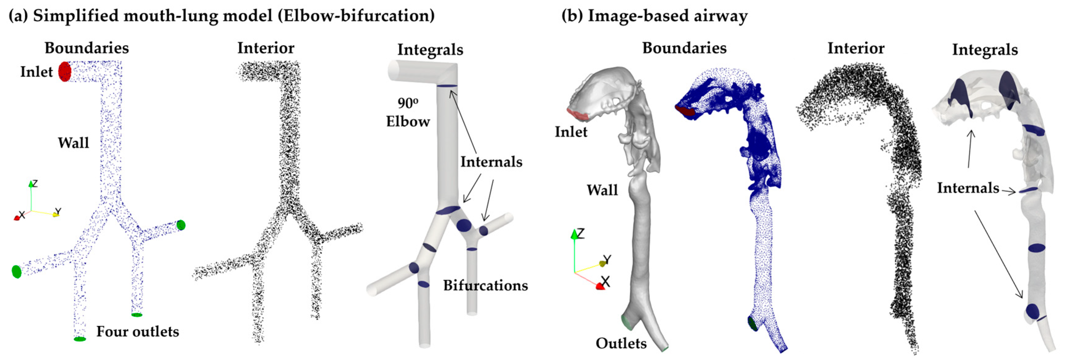
Figure 2.
Flowchart of physics informed neural network (PINN) training and visualization: (a) problem specification and model training with essential steps (dotted block) and potential pitfalls (bold within blocks), and (b) visualization/validation using ParaView, ANSYS Fluent, and Tecplot.
Figure 2.
Flowchart of physics informed neural network (PINN) training and visualization: (a) problem specification and model training with essential steps (dotted block) and potential pitfalls (bold within blocks), and (b) visualization/validation using ParaView, ANSYS Fluent, and Tecplot.
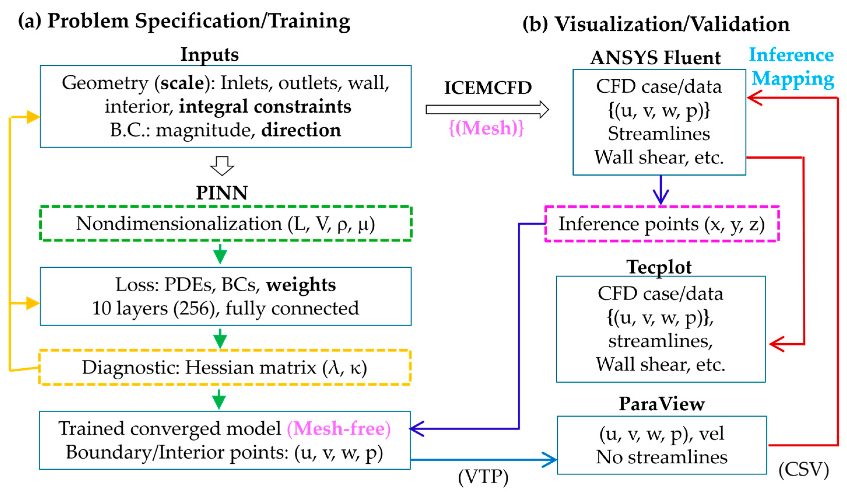
Figure 3.
Comparison of duct flows in terms of pressure and velocity contours predicted by (a) PINN laminar model, (b) ANSYS Fluent laminar model, and (c) PINN-CFD differences.
Figure 3.
Comparison of duct flows in terms of pressure and velocity contours predicted by (a) PINN laminar model, (b) ANSYS Fluent laminar model, and (c) PINN-CFD differences.
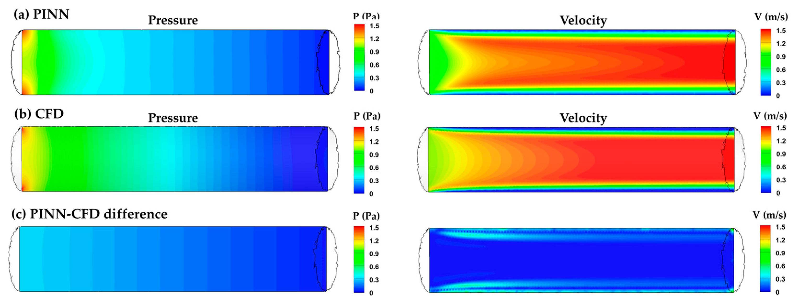
Figure 4.
PINN training diagnosis using the condition number κ of the Hessian matrix of the loss functions vs. inlet velocity and geometrical complexity: (a) mean κ, and (b) maximum κ. Note the different scales in the y-axis.
Figure 4.
PINN training diagnosis using the condition number κ of the Hessian matrix of the loss functions vs. inlet velocity and geometrical complexity: (a) mean κ, and (b) maximum κ. Note the different scales in the y-axis.
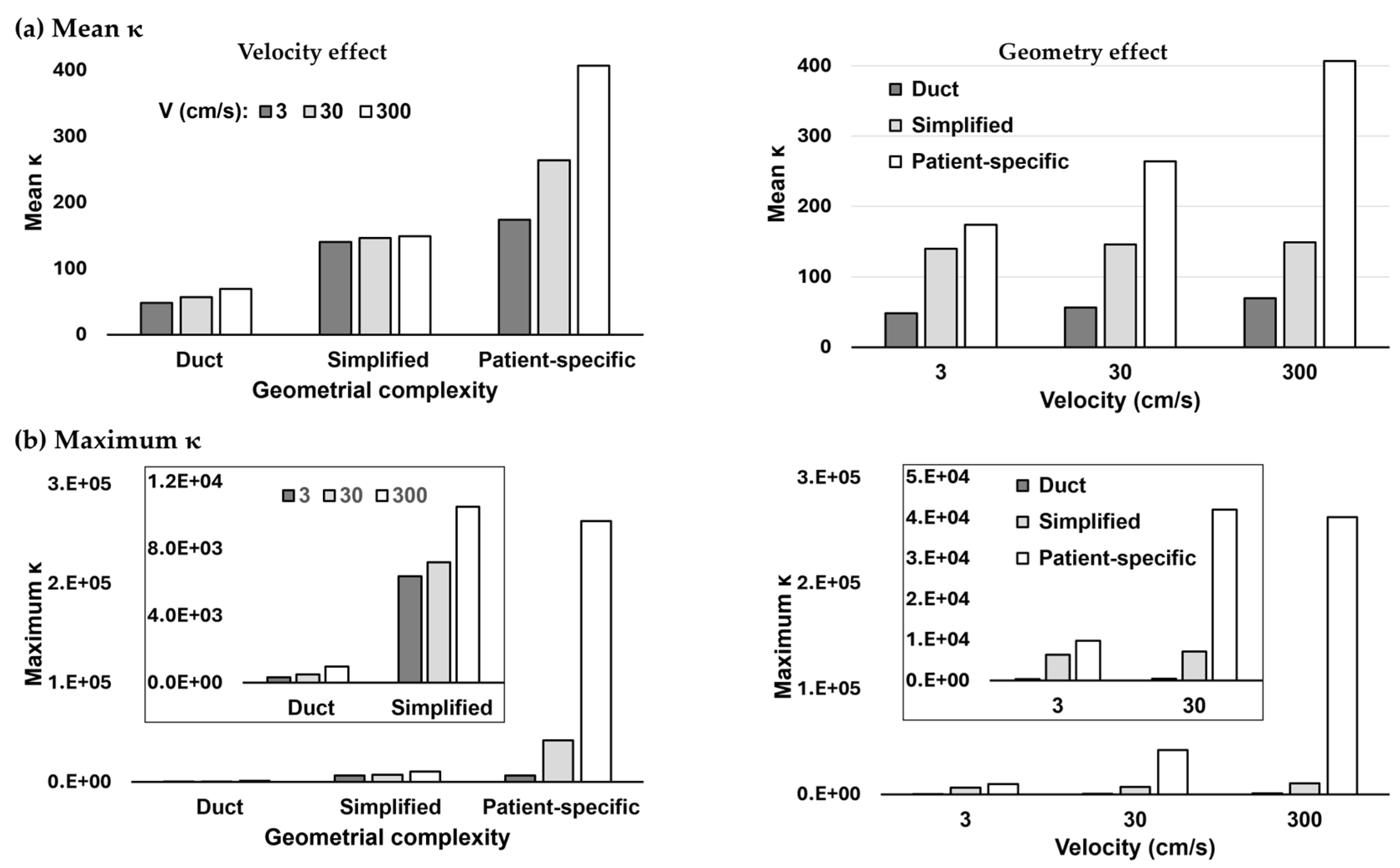
Figure 5.
Comparison of airflows in the simplified airway in terms of pressure, velocity, wall shear, streamline, and Q-criterion predicted using: (a) PINN laminar model, and (b) ANSYS Fluent laminar model.
Figure 5.
Comparison of airflows in the simplified airway in terms of pressure, velocity, wall shear, streamline, and Q-criterion predicted using: (a) PINN laminar model, and (b) ANSYS Fluent laminar model.
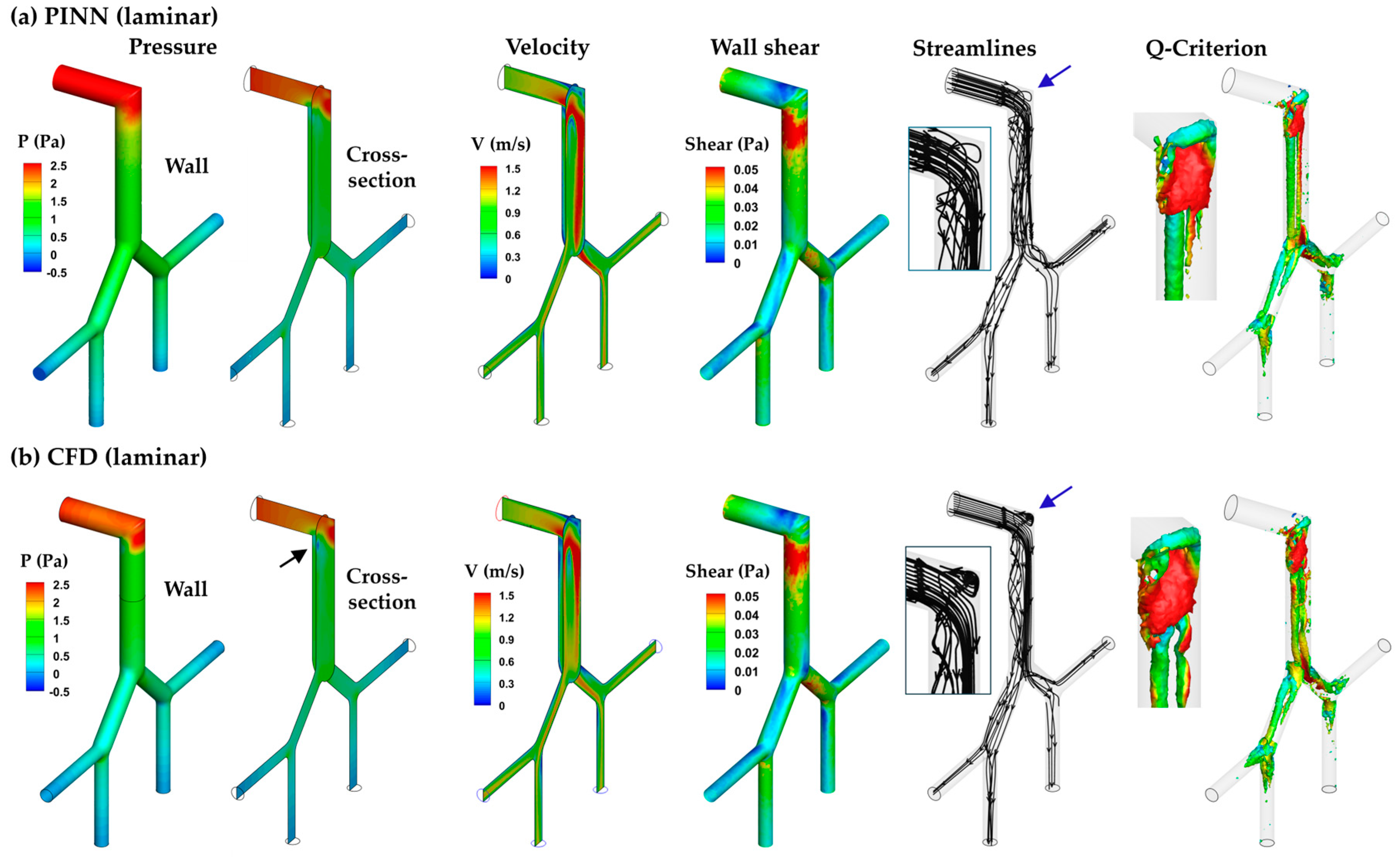
Figure 6.
PINN-CFD differences (laminar model) in the simplified airway: (a) pressure, and (b) velocity.
Figure 6.
PINN-CFD differences (laminar model) in the simplified airway: (a) pressure, and (b) velocity.
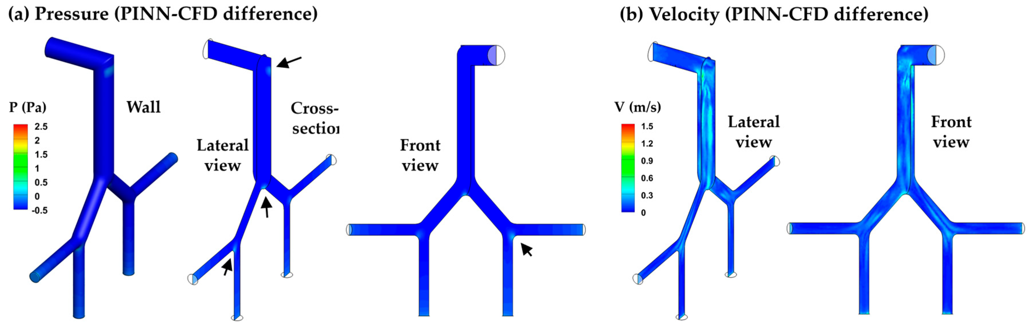
Figure 7.
Comparison of airflows in the simplified airway predicted by the SDF-mixing-length PINN and ANSYS Fluent k-ω turbulence model: (a) velocity fields, and (b) streamlines.
Figure 7.
Comparison of airflows in the simplified airway predicted by the SDF-mixing-length PINN and ANSYS Fluent k-ω turbulence model: (a) velocity fields, and (b) streamlines.
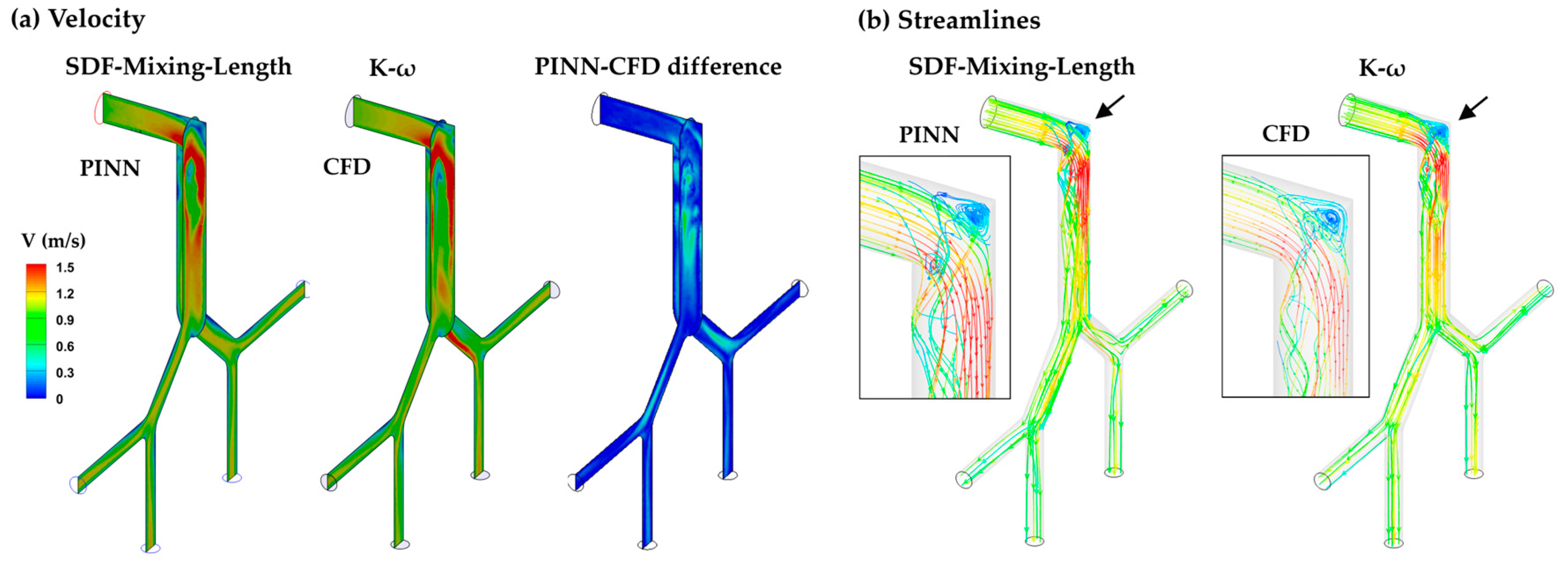
Figure 8.
PINN laminar model vs. CFD in the patient-specific upper airway model at an inlet velocity of 1 m/s: (a) PINN predictions of streamlines, velocity, pressure, and wall shear stress, and (b) corresponding predictions from the laminar model in ANSYS Fluent.
Figure 8.
PINN laminar model vs. CFD in the patient-specific upper airway model at an inlet velocity of 1 m/s: (a) PINN predictions of streamlines, velocity, pressure, and wall shear stress, and (b) corresponding predictions from the laminar model in ANSYS Fluent.
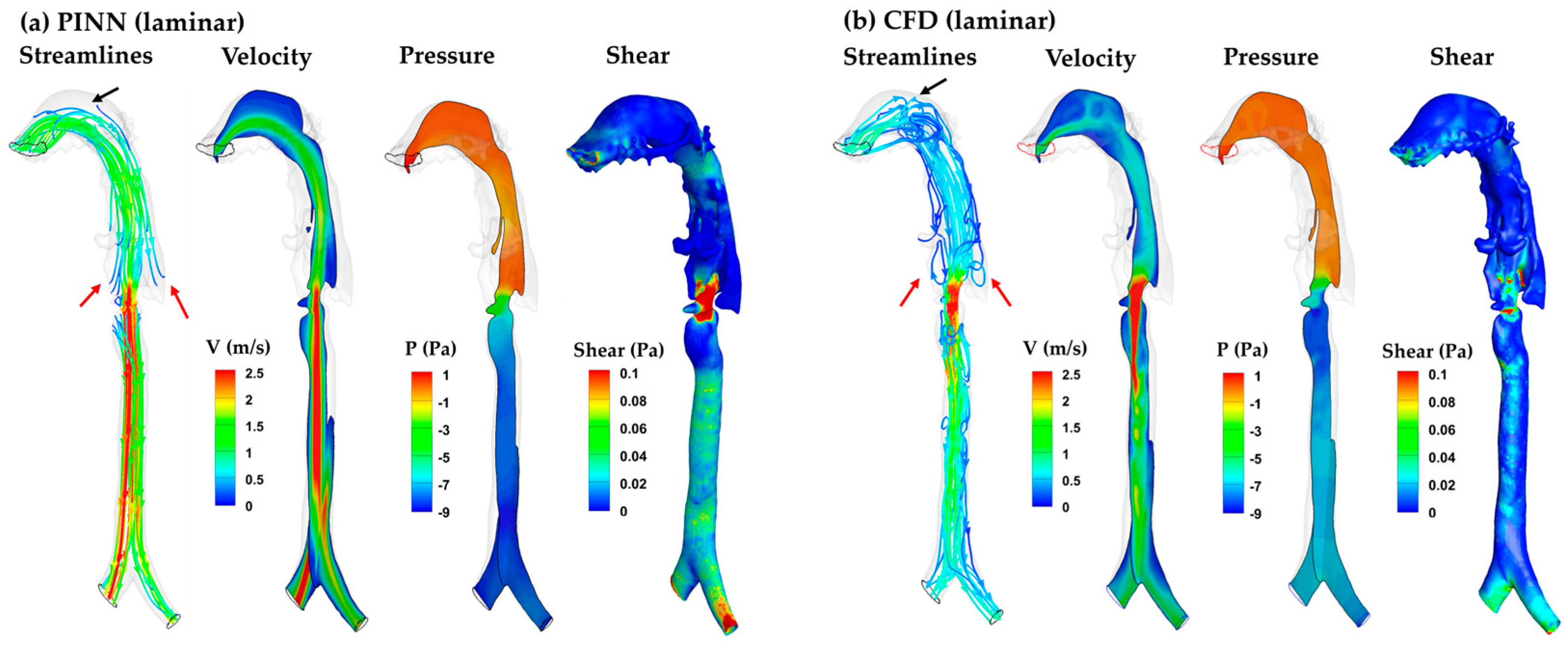
Figure 9.
PINN turbulence model vs. CFD in the patient-specific upper airway model at an inlet velocity of 1 m/s: (a) PINN mixing length model predictions of streamlines, velocity, pressure, and wall shear, and (b) corresponding predictions using the k-ω turbulence model in ANSYS Fluent.
Figure 9.
PINN turbulence model vs. CFD in the patient-specific upper airway model at an inlet velocity of 1 m/s: (a) PINN mixing length model predictions of streamlines, velocity, pressure, and wall shear, and (b) corresponding predictions using the k-ω turbulence model in ANSYS Fluent.
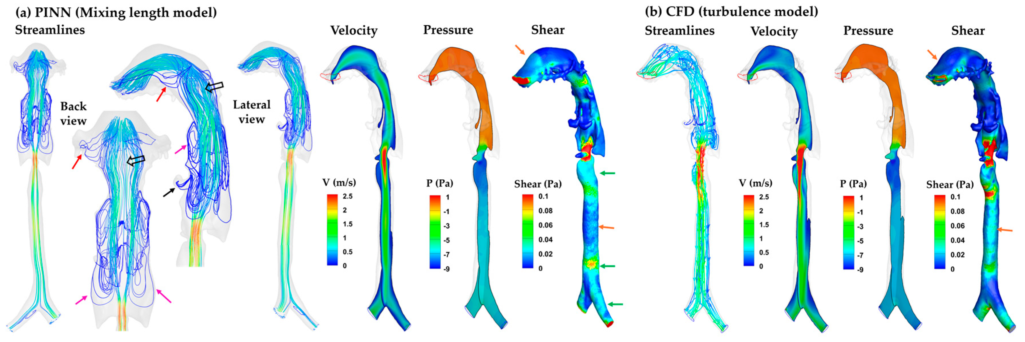
Figure 10.
Evaluation of the relative significance of the SDF-mixing-length PINN model: (a) PINN-CFD differences in velocity and pressure, (b) PINN-based turbulent viscosity ratio, µt/µlam, on the inference points (3.6 million, same as CFD cell number), and (c) signed distance function (SDR) on the interior training points (6,000).
Disclaimer/Publisher’s Note: The statements, opinions and data contained in all publications are solely those of the individual author(s) and contributor(s) and not of MDPI and/or the editor(s). MDPI and/or the editor(s) disclaim responsibility for any injury to people or property resulting from any ideas, methods, instructions or products referred to in the content. |
© 2025 by the authors. Licensee MDPI, Basel, Switzerland. This article is an open access article distributed under the terms and conditions of the Creative Commons Attribution (CC BY) license (http://creativecommons.org/licenses/by/4.0/).
Copyright: This open access article is published under a Creative Commons CC BY 4.0 license, which permit the free download, distribution, and reuse, provided that the author and preprint are cited in any reuse.


