
Submitted:
28 October 2025
Posted:
29 October 2025
You are already at the latest version
Abstract
We recap the theory of diffeomorphisms and covariances acting on a space and their induced action on fields, and how this leads to their decomposition into Fourier modes and harmonics. We show that a careful consideration of this theory reveals some unexpected results. For a start, harmonics are distinguished by their ‘quantum numbers’, but this analysis is valid for classical fields, so that classical fields can be written as a linear sum of modes with ‘quantum numbers’. Furthermore, certain models of compactification, as described in previous works by the author, are found to exploit a loophole in a key ‘no-go’ theorem, allowing the Poincaré group and an internal O(N ) symmetry group to be embedded in a larger symmetry group. This embedding is achieved without the need for the fermionic generators of supersymmetry and it is manifest in the ‘decompactification limit’. Away from this limit – for a realistic universe – the homogeneous part of this larger symmetry group is non-linearly realised. The translation part of the original symmetry group is realised as additional rotational transformations on the compact factor space.
Keywords:
Diffeomorphisms
; covariances
; harmonics
; eigenfunctions
; periodicity
; quantum numbers
; compactification
; Kaluza-Klein
; no-go theorems
; Lie algebras
; group theory
; translations
; rotations
; Poincaré group
; unification
; non-linear realisations
; geometry
; N-spheres
; product spaces
1. Introduction
1.1. How Periodicity Results in Quantization
When de Broglie first proposed the idea of a quantum wavefunction, he showed how the periodicity of a closed path in space could lead to a quantity being quantized. Sommerfeld had worked with Bohr’s model of the atom, in which electrons moved in specified orbits around the nucleus. He had shown that for circular or elliptical orbits, quantization of the action was equivalent to quantization of the component of angular momentum in the plane of the orbit [1]. De Broglie pointed out that if a wave was associated with an orbiting electron, “it is physically obvious that to have a stable regime... the points of a wave located at whole multiples of the wavelength l, must be in phase”. To illustrate this point, he used water waves in an annular channel as an analogy. This condition gave exactly Bohr’s formula for electron orbits [2].
This picture was quickly superseded by a three-dimensional one, in which atomic orbitals are harmonics on a foliation of three-space into concentric two-spheres, found as simultaneous eigenfunctions of the operators and . This theory can be found in quantum mechanics textbooks (such as [3]) and summarised in Section 4.3.
The full relativistic treatment was set out in a paper by Wigner published in 1939 [4]. This classified the unitary representations of the Poincaré group (“the inhomogeneous Lorentz group”) with non-negative energy. It does this by looking at the action of the (homogeneous) Lorentz subgroup on massive and massless states, with a momentum four-vector which is either timelike or null. It identifies the stabiliser groups for each type of state – crucially, by taking the action of the Lorentz group to be that of unitary operators acting on fields. It then looks at the quantum numbers associated with these stabiliser groups.
Note that all three of these analyses are carried out in three dimensions of space and one of time. Where they differ is that de Broglie’s analysis looks at waveforms with rotational symmetry in two dimensions, the analysis using and looks at waveforms with rotational symmetry in three dimensions and Wigner’s analysis looks at the symmetries of states under Lorentz and Poincaré transformations.
However, in 1926, just two years after de Broglie’s hypothesis of matter waves, an analysis was published with an additional dimension. In 1921, Kaluza [5] had taken General Relativity and cast it in five dimensions. He had shown that curvature of a five-dimensional spacetime could be manifested as both gravity and electromagnetism. Klein was captivated by both this idea and de Broglie’s matter waves. With a slight modification of Kaluza’s proposal [6], he showed how de Broglie’s matter waves could be incorporated into the five-dimensional picture, resulting in “the equation given by Schrödinger, whose standing waves correspond, as known, to the values of E which are identical to the energy values calculated from Heisenberg’s quantum theory” [7]. Indeed, he argued that the quantum theory of de Broglie, Schrödinger and Heisenberg was more natural in five dimensions, and his paper emphasised the notion of a complex phase factor of the wave.
Later the same year, in a very short letter to Nature, he explained that if the extra dimension is periodic, the generalised momentum corresponding to its coordinate is quantized. For a particle with an electric charge, its charge is proportional to this generalised momentum; hence, periodicity in the extra dimension implies that a particle’s charge must be an integer multiple of a basic quantum [8]. (See [9] for an extensive history of these topics.) The states with different electric charges are Fourier modes on the loop-like extra dimension [10].
Taken together, the above body of theory shows how classical field configurations on a compact space can be decomposed into complex linear sums of harmonics – a point we emphasise in Section 4. These harmonics are distinguished and labelled by quantum numbers. Hence a compact space leads naturally to quantization. This has significant implications. The one we focus on in this paper is the implication for unification theories with more than four dimensions.
1.2. Routes to Unification and No-Go Theorems
When de Broglie, Klein and others were developing their ideas, gravity and electromagnetism were the only fundamental interactions which were known and understood with any clarity. However, over time, research into nuclear structure, nuclear beta decay and cosmic rays provided evidence for the nuclear interactions. Over the following decades, the conceptual advances of gauge theories, the quark model and spontaneous symmetry breaking allowed a theoretical understanding of the strong and electroweak interactions to develop. By the end of the 1960s, both were understood as quantum field theories.
In quantum chromodynamics, the strong force is understood as a quantized gauge field. Meanwhile, in electroweak theory, the gauge group of electromagnetism forms as a subgroup of a larger gauge group, . Transformations under this larger group act linearly on fields at high energies, but at lower energies, its symmetries are spontaneously broken, with only the gauge symmetries remaining manifest.
The success of electroweak unification (and before that, the unification of electricity and magnetism) led physicists to wonder if further unification of the forces was possible. The main method examined for this was choosing a gauge group which contained both and as subgroups, then examining how this group may be spontaneously broken at low energies to the two subgroups. These models were known as Grand Unified Theories (GUTs).
The mathematics of this looked plausible, so physicists wondered whether the gauge group could be extended again to incorporate the Poincaré group of spacetime symmetries, thereby paving the way for unification with gravity.
In the 1960s, a series of no-go theorems were published which seemed to rule out combining Poincaré group symmetries with internal symmetries in anything but a trivial way (as a direct product). The most famous of these theorems nowadays is that due to Coleman and Mandula [11]. This was based on the symmetries of the S-matrix and was constructed to be valid for many particle states and for infinite-dimensional groups.
In this paper, we consider its predecessor, O’Raifeartaigh’s no-go theorem [12]. This is based on arguments concerning Lie algebras. Unlike the Coleman-Mandula no-go theorem, it does not cover cases in which the embedding algebra is infinite-dimensional. This is not a problem for us, as we are concerned in this study with strictly finite-dimensional algebras. As we are studying the configurations of fields rather than the dynamics of particles, this seems the more appropriate of the two to focus on.
We show how certain models of compactification described in [13,14] exploit a loophole in this theorem. This is done without needing supersymmetry (for which there is no evidence at a fundamental level). We describe how the larger algebra in which the internal symmetry algebra and the Poincaré algebra are embedded is only manifest in a particular limit, corresponding to flat higher-dimensional spacetime. In this limit, there would be – as pointed out by O’Raifeartaigh – extra quantum numbers associated with higher-dimensional translations, with continuous spectra. However, in the universe we actually inhabit, all the additional symmetries are non-linearly realised. The translations and rotations in the extra flat dimensions are replaced by rotations on a (possibly squashed or stretched) sphere. There is at most one generator which commutes with those of the Poincaré algebra and the internal symmetry algebra, which has discrete quantum numbers.
Consequently, the fields in these models of compactification – such as the metric, the velocity vector field , the Ricci tensor and various scalar and tensor fields that can be constructed out of these – may be decomposed in harmonics which carry the quantum numbers of the Poincaré algebra and the internal symmetry algebra, and, depending on the number of extra dimensions, perhaps one further quantum number.
1.3. Structure of This Paper
To understand this issue of how the compactification models relate to O’Raifeartaigh’s theorem, a thorough grasp is needed of diffeomorphisms, covariances, their induced actions on vector fields, periodicity and harmonics. Most physicists have a reasonable working knowledge of these subjects, but there are significant subtleties that could be missed, so the majority of this paper is recapping established geometry. This is done as follows.
In Section 2, we briefly recap the meaning of diffeomorphisms and covariances, providing the examples of rotations and translations in Euclidean space. In Section 3, we look at actions these induce on fields, using vector fields as examples – `dragging actions’, changes of coordinate basis on tangent spaces and changes of functional form. We identify generators for these actions. In Section 4, we look at scalar and vector field configurations which are symmetric under the induced actions, on both compact and non-compact spaces. This allows us to define eigenfunctions of the generators, and again we focus on the examples of rotations and translations.
While this theory is all widely known in outline, the consequences are far-reaching, even the immediate ones. It does not seem to be widely recognised, for example, that classical fields can be decomposed into harmonics which are eigenfunctions of operators, each with a unique set of eigenvalues.
Finally, in Section 5, we apply all this theory to the case of the models of compactification contained in [13,14]. We start with some commentary on no-go theorems, particularly those of O’Raifeartaigh and Coleman and Mandula, then we recap the classification scheme used by O’Raifeartaigh. After summarising the compactification models of [13,14], we describe a coordinate system for the compact factor space of additional dimensions, based on that used by Gell-Mann and Lévy and Meetz [15,16]. After this, it is fairly simple to explain how the models of compactification fall within a loophole in O’Raifeartaigh’s no-go theorem.
We summarise all of the earlier sections in Section 6, mentioning in passing some cases in which the principles of this paper apply more broadly than in the limited illustrative examples provided here.
2. Diffeomorphisms and Covariances
We start with a pair of definitions. These are well-known in the literature on geometry, but nonetheless, sometimes get misused - physicists sometimes use the term diffeomorphism when they are actually referring to covariances.
A diffeomorphism is a is a bijective map which maps each point on a manifold to a specific point on another manifold. We are interested in automorphic diffeomorphisms – ones which map each point on a manifold another point on the same manifold. If we have a set of such maps, we can combine any pair of them, simply by considering the initial and final points of the combined maps - as shown in Figure 1.
With this rule for combining maps, the set of all diffeomorphisms forms a group, . These are active transformations on .
A covariance on a coordinate neighbourhood of is a change of coordinate system on that coordinate neighbourhood - a passive transformation. Again, by carrying out two changes of coordinate system consecutively, we get a third covariance, so we have a rule for combining them. And again, the set of all covariances forms a group.
Indeed, for each diffeomorphism on a coordinate neighbourhood there is a corresponding covariance. Hence the covariance group and diffeomorphism group are isomorphic.
We can illustrate this correspondence using translations and rotations on Euclidean space.
2.1. Translations
Consider a translational diffeomorphism f on a Euclidean space with Cartesian coordinates . This maps every point on the space to another point. We illustrate this in Figure 2 for just two points, A and B. In this example, each point is mapped three units to the right. Point A, for which , is mapped to , for which ; its other coordinate values remain the same. Similarly, B with is mapped to with . Thus
The corresponding covariance is shown in Figure 3. A and B stay where they are, but now the x-axis is shifted three units to the left, giving us a new coordinate. The other coordinates remain the same. Thus
The relationship between these two maps is clearly that A and B have the same values of the coordinates that and have in the original coordinate system.
2.2. Rotations
Now consider a rotation R in the x-y plane through an angle , as shown in Figure 4. (Other axes not shown – they are orthogonal to the x- and y-axes.) This maps each point to another one, according to the rule
The corresponding covariance is shown in Figure 5. A and B stay where they are, but now the x- and y-axes are rotated through an angle of anticlockwise.
The new coordinates take the form
Both of these are simpler in polar coordinates:
These show that a rotation is a shift of the angular coordinate , just as a translation is a shift of the Cartesian coordinates.
3. Induced Actions on Vectors and Fields
Diffeomorphisms and covariances both have induced actions which can most clearly be illustrated using vector fields.
3.1. Dragging Action
A diffeomorphism on a manifold induces an active transformation on a field, by `dragging’ the field along with it. Indeed, this is sometimes known as a `dragging action’ [17].
For a vector field , this plays out as follows. If a diffeomorphism f maps a point P to a point :
then the induced transformation takes the field at P and moves it to the point . This mapping is applied to the vector at each point in the region under consideration, giving us a new vector field, :
We now want to analyse how these fields, and , are related. This is simplest when each point is displaced by the same small amount along one coordinate direction, as we can then use a simple Taylor expansion. For example, Figure 6 shows an active translation of a vector field to the right.
If we denote the displacement , then has a value at a point which is the same as the value of at a point :
or in general
This may be expressed in terms of the differential operator with respect to x:
The expression in brackets is a power series in the operator - that is, generates translations.
There is a similar dragging action under a rotation. To make sure that a rotation diffeomorphism (as shown in Figure 4 above) is described by a global displacement along one coordinate direction, we adopt polar coordinates for the plane in question. Then under a rotation through , has a value at a point which is the same as the value of at a point . Applying the same arguments as for translations, we find:
Thus we find that generates rotations. This can be expressed in Cartesian coordinates in the well-known form
Note the similarity between our transformation generators and the quantum mechanical operators for linear momentum and orbital angular momentum. In natural units, these differ only by a factor of i.
3.2. Transformation of a Vector Field Under Changes of Coordinates
For covariances, it is easiest to start by looking at a vector at a single point.
We may decompose a point vector into components in a coordinate basis corresponds to a set of coordinates :
A change of coordinates
will, in general, induce a transformation of the coordinate basis:
The vector remains the same, but can be decomposed in either basis:
We can thus find the way the components in the new basis relate to those in the original basis:
In most cases, the new components will differ from the original components. For example, when we are using Cartesian coordinates and considering rotations about the origin, the Jacobian matrix elements in (20) are:
However, if the new coordinates differ from the original ones simply by adding constants, the basis remains the same, and therefore so do the components [19]. As we saw in previous sections, this is the case both for translations in Cartesian coordinates and for two-dimensional rotations in polar coordinates.
This principle carries over to vector fields. For a field in a given coordinate system, the value at a given point can be decomposed into components associated with the coordinate basis at that point. This is shown in Figure 7.
Under a change of coordinates, in general this decomposition changes, as shown by comparing Figure 7 with Figure 8.
However, if the basis does not change under a coordinate transformation, neither do the values of the components.
But even in this case, what may change is the way these components are expressed as functions of the coordinates. For example, the vector field shown in Figure 7 is
The point A has coordinates . At this point, the x-component of V is therefore , while the y-component is 12. Now choose a new x-coordinate by adding 3 to the existing one:
Then can be expressed in terms of the new coordinate system as:
For the point A, the new coordinate has a value of 5. But the values of the components haven’t changed:
Similarly, consider a vector field
and its value at a point A with coordinates
Thus
We now construct a new angular coordinate by adding to the existing one:
so that A has coordinates
This preserves the basis vectors, but changes the functional form of the angular component to
but its value at A remains .
Just as for the diffeomorphisms, it is possible to express such a change as a Taylor expansion. If a component of a vector field is an analytic function of the original coordinates , then this component can be expressed in terms of the new coordinates, , using a Taylor series. Each term contains a higher-order derivative of the analytic function.
For example, if
then under
we find
where is the derivative of f with respect to its first argument:
and so on for higher derivatives. We can see that this has the same essential form as (11).
4. Periodicity, Eigenfunctions, Eigenvalues and Harmonics
The preceding considerations allow us to define symmetries for a field configuration under diffeomorphisms and covariances. If, under a diffeomorphism on a manifold
a field configuration is preserved under the corresponding dragging action:
we say that the field configuration is symmetric under this action. The corresponding covariance preserves the functional form of the field. This definition of the symmetry of a field configuration is valid for scalar fields, spinor fields, vector fields and higher-rank tensor fields (although for non-scalar fields under covariances, consideration needs to be given to whether there are changes of basis, as this affects how it is resolved into components).
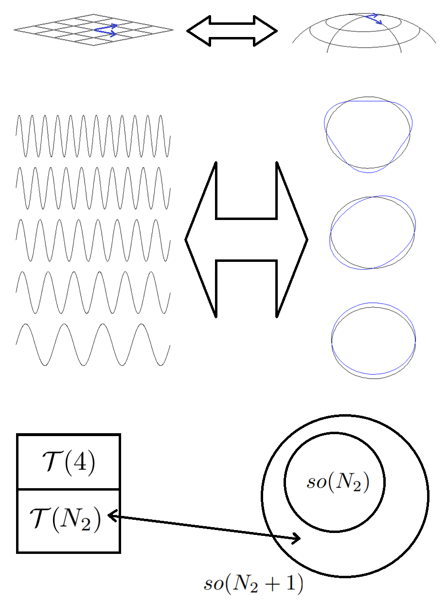
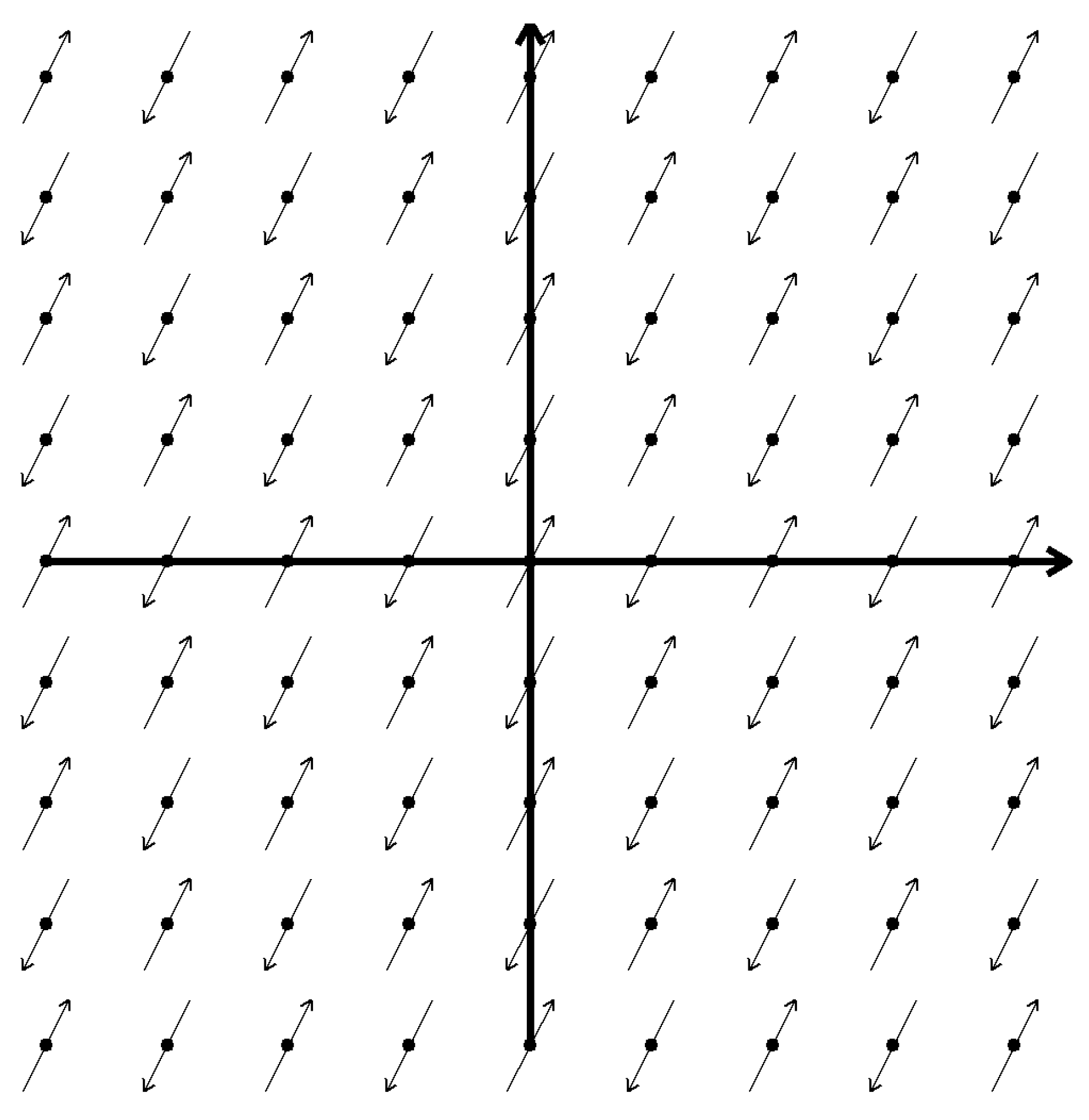
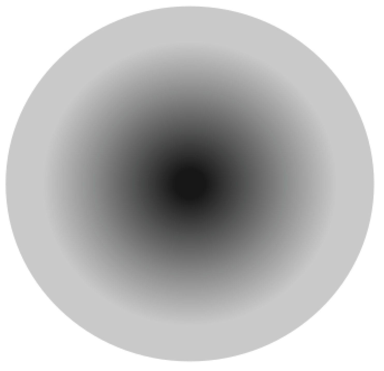
For example, Figure 9 shows a scalar field which is symmetric under a four-fold discrete rotational symmetry, while the scalar field in Figure 10 has discrete translational symmetries. Figure 11 shows a vector field which has rotational symmetries and Figure 4 shows a vector field which has translational symmetries.
Figure 12.
Vector field with translational symmetries.
Particular examples of such symmetries can be found in the literature. For example, isometries are symmetries of the metric field, while Hohmann et al examine transformations under which both the metric and the Weitzenböck connection are form-invariant [18].
For simplicity, we will focus on scalar fields.
4.1. Subgroups of the Diffeomorphism Group on Compact and Non-Compact Manifolds
Above, we considered rotations in a plane of a Euclidean space. These form a continuous one-parameter subgroup of the diffeomorphism group. Field configurations with rotational symmetry, such as that in Figure 9, are symmetric under such transformations through particular angles about the centre of the configuration. Similarly, translations along an axis of a Cartesian coordinate system form a continuous one-parameter subgroup of the diffeomorphism group. Under the associated dragging action, a field configuration such as that in Figure 10 is symmetric under particular values of the parameter.
In both these cases, the symmetry amounts to a periodicity in a coordinate. However, they differ in that a path generated by a rotation forms a closed, finite loop, while a translation group generates an infinite, open path.
In general, whether both types of transformation exist depends on the shape of the manifold. On , they clearly exist: we can adopt Cartesian coordinates and then translations are simply additions to the coordinates. These form a non-compact group. For , there are also compact groups of diffeomorphisms.
On , on the other hand, translations do not exist. We cannot put Cartesian coordinates on it, while if we use angular coordinates, the coordinate curves are closed loops. Displacements along these are rotations.
For a non-compact group of diffeomorphisms, field configurations may have any period.
For a compact group of diffeomorphisms, on the other hand, there are only particular allowed values of the period. For example, say that on rotating a field configuration about its centre, it repeats after an angle of - that is, is the fundamental period under such rotations. Then must be a multiple of the period:
For any positive integer value of n, it is possible to envisage a field configuration which has the corresponding period. For example, the field configuration in Figure 9 has four lobes. It therefore has . If these were replaced by eight lobes, it would have . A configuration with would be symmetric under the full rotation group, for example as shown in Figure 13. Otherwise, the field configuration is symmetric under a discrete subgroup of the rotation group.
4.2. Eigenfunctions and Eigenvalues of Translations
Under a translational diffeomorphism, the induced map on a scalar field will take a form similar to that given above for a vector component:
where the differential operator generates the translation.
Usually, the new field is different from the original one.
But consider the case where the field is an eigenfunction of the generator:
(40) is solved by
In this case, the induced transformation simply scales the field:
In particular, if and are related by
for any , is invariant under the translation:
This means that a translation through is a symmetry for a field configuration of the form
Thus for each displacement , we have an infinite series of eigenvalues, and corresponding to each, there is a function which is symmetric under translations through that interval.
This theory is valid in both classical field theory and quantum theory. However, these functions which are symmetric under translations are complex-valued. They therefore cannot represent any physical fields which are directly observable. For example, temperature or pressure in a box cannot be complex-valued.
Where they are useful is in Fourier analysis. Any complex linear sum of these symmetric fields is also symmetric under a translation through . As is well-known, they form a basis for fields, including real fields, which are symmetric under this transformation and satisfy Dirichlet conditions.
We can also use these basis states for analysing covariances. Under a change of coordinates from x to , the functional form is preserved for any field configuration which is a complex linear sum of the basis states.
Note that translations in the directions are generated by , . These partial derivatives commute, so a field configuration may simultaneously be an eigenfunction of all of these. For example, with three dimensions, any configuration of the form
where , is an eigenfunction of all three operators. Any values of will provide an eigenfunction; we can see that if they are all imaginary, then for any set of these values, there is always a choice of , and under which it is preserved – the operators are Abelian and their spectra are continuous.
4.3. Eigenfunctions and Eigenvalues of Rotations
Under a rotational diffeomorphism through an angle , the induced map on a scalar field is clearly:
The eigenfunctions of the generator take a very similar form to those of the translation generator:
However, for each of the components to be single-valued, we need it to be unaffected by adding to the coordinate. For an eigenfunction, we find that this implies that the eigenvalue is an integer multiple of :
If our space has more than two dimensions, there is more than one plane of rotations, hence more than one generator. Not all of these generators commute – this depends on whether the planes corresponding to two generators share a common direction. For example, rotations in the plane, generated by , commute with rotations in the plane, generated by . However, none of these commute with rotations in the plane.
In three dimensions, a field configuration can only be an eigenfunction of at most one generator. As is well known, there is also a quadratic Casimir operator which commutes with all three generators. If we choose the generator of rotations around the z-axis, the simultaneous eigenfunctions of this and the Casimir operator are the spherical harmonics which are familiar from quantum mechanics, multiplied by a purely radial function. In spherical polar coordinates, these take the form
Under the action of the quadratic Casimir, these satisfy
where l is a non-negative integer – for this is required for to be finite for all [3]. is clearly the eigenvalue of
From the solution, solution for other values of m can be found. One can then define the well-known ladder operators as complex linear sums of and and use these to show that for a given value of l, m can range from –l to l.
For or , where N is the number of dimensions and p is an integer, there are p mutually commuting generators. Harmonics may also be defined for these higher-dimensional spaces.
Note that although these harmonics are labelled using `quantum numbers’, they may be defined for classical scalar fields. Just as a classical field in may be decomposed into Fourier modes, each of which has eigenvalues associated with the translation generators, a classical field in can be decomposed into harmonics, each of which has eigenvalues associated with the mutually commuting rotation generators. For example, the temperature across the globe at a given moment in time can be decomposed into linear sums of harmonics with values of m and l. However, unlike the translations, the operators for rotations are non-Abelian and have discrete eigenvalues.
5. O’Raifeartaigh’s No-Go Theorem and Compactification
5.1. No-Go Theorems
Having established this theory on harmonics and quantum numbers, we now turn to its implications for unification in Kaluza-Klein theories.
As explained in Section 1, by the early 1960s, physicists were considering how the quantum field theories of QED and QCD could be unified with gravity. It was rapidly found that there were various technical problems with trying to combine Poincaré symmetries and internal symmetries. These were published in the form of `no-go theorems’ in 1964 and 1965. These culminated in papers by O’Raifeartaigh [12] and Coleman and Mandula [11], which provide references to around ten earlier papers in this investigation.
The Coleman-Mandula theorem is based on the symmetries of the S-matrix – considering unitary operators which commute with it, turn one-particle states into one-particle states and act “on multi-particle states as if they were tensor products of one-particle states”. These form a group, but there is no assumption that this group has a finite number of generators. Coleman and Mandula saw this validity for infinite-dimensional groups as an advantage of their no-go theorem over previous ones, and this may be at least partly why it has become the most commonly cited of the theorems.
This theorem essentially says that if a group of internal symmetries satisfies the required properties, it can only be embedded in a larger group alongside the Poincaré group if that larger group is simply a direct product of the two. The only exception to this rule that has been established is supersymmetry.
O’Raifeartaigh’s theorem, on the other hand, takes a purely group-theoretic approach to the problem. More precisely, it considers the Lie algebras of the Poincaré group and a group of internal symmetries –- this makes its conclusions valid for any representations of these groups. It considers how these two Lie algebras may be embedded in a larger, but finite, Lie algebra.
As we are concerned in this study with strictly finite-dimensional algebras and we are studying the configurations of fields rather than the dynamics of particles, this is the theorem on which we shall focus.
5.2. O’Raifeartaigh’s Classification of Algebra Embeddings
O’Raifeartaigh showed that there are four ways that the Lie algebra of the Poincaré group might be embedded in a Lie algebra . To do this, he used Levi’s radical-splitting theorem, which states that is the semidirect product of a semisimple Lie algebra and an invariant solvable subalgebra . The four ways are:
- (i)
- is the algebra of translations in four-dimensional spacetime ;
- (ii)
- is Abelian and contains (but is larger than) ;
- (iii)
- is solvable but not Abelian and contains ;
- (iv)
- .
For case (i), he showed that if contains the semisimple Lie algebra of an internal symmetry1, then
For case (ii), he showed that all the elements of S commute with both each other and all the elements of . This implied that they represent `internal quantum numbers which can be measured simultaneously with momentum and energy’. In general, the spectra of such operators would be continuous. This, he stated `is not easy to interpret physically’. He concluded that `case (ii) cannot be ruled out, but it is also not particularly attractive’.
For case (iii), he pointed out that `solvable non-Abelian algebras are not usually considered in physics’, partly because every finite-dimensional representation is triangular. This means that Hermitian conjugation for such representations cannot be defined.
For case (iv), the entire Poincaré algebra is embedded in a simple Lie algebra. This is only possible if the translation generators are complex combinations of the generators of the compact form of the Lie algebra within which the Poincaré algebra is embedded. This `may lead to serious difficulties in defining multiplets’.
O’Raifeartaigh’s theorem generally rules out non-supersymmetric unification in which gauge symmetries in four dimensions are broken by spontaneous symmetry breaking.
It might naively seem that it also rules out non-supersymmetric Kaluza-Klein unification. This has widely been assumed by researchers –- for example, during a busy period of research on such theories in the early 1980s, much of the research aimed at eventually building in supersymmetry. However, for at least some theories in which extra dimensions form a compact space, this is not actually the case, as we now explain.
5.3. The Spacetime of Covariant Compactification
At this point, it is worth specifying the type of theory we will consider in this section. This type of theory is described in my earlier works [13,14].
The additional dimensions are real, physical ones, forming a compact manifold. To make things simple, we will take this to be , where is the number of additional dimensions (adopting the notation of [13]). However, heuristic reasoning suggests that the same theory should be simple to extend to any compact manifold homeomorphic to . The whole spacetime forms a product of this compact space and a four-dimensional spacetime. The theory has a classical vacuum which is a Cartesian (direct) product of the two factors, but in the presence of matter, this deforms into a more general product of the factors.
One can also take a mathematical `decompactification’ limit, in which the curvature of both factor spaces reduces to zero. In this limit, the spacetime reduces to , where N is the total number of dimensions of the spacetime. There is a homomorphism from the covariance group for this flat spacetime to the group of (Jacobian) matrices which act on the coordinate basis for a tangent space at a given point [19]. These matrices form the group . The homogeneous part of this is , where t is the total number of time dimensions and s the total number of space dimensions.
Away from this limit, the group and its subgroup are both non-linearly realised. However, the general linear groups and (pseudo-)orthogonal groups relating to each of the factor space remain linearly realised. On the product space, one can define coordinate systems which respect the factor manifolds: one subset of the coordinates, , parametrizes the familiar four-dimensional spacetime and the remainder, parametrize the other factor space. In these coordinates, all tensors of the full N-dimensional spacetime decompose into tensors of the two factor spaces.
5.4. Sigma-Model Coordinates
On the compact space of extra dimensions, we will adopt a specific coordinate system which is particularly well suited to our purposes. We will call this coordinate system `sigma-model coordinates’, as these are based on a coordinate system used in the paper which first set out a non-linear sigma model [15], and also in the paper which first calculated a metric for such coordinates [16].
Let us start with the familiar two-sphere. We can embed in three-dimensional Euclidean space. Its intersection with the z-axis – the `North pole’ point – is stabilised by an subgroup of the rotation group. This is a one-parameter subgroup. Rotations involving the other two parameters of map the `North pole’ to each of the other points on the two-sphere.
We can find the x and y coordinates of any point on the Northern hemisphere by projecting down onto the equatorial plane. We will call the corresponding coordinates on the sphere and . Thus, the Cartesian coordinates of this point in are:
We can use the embedding into to find a metric for the Northern hemisphere in these coordinates [20]:
(where due to the positive definite signature). We can also look at the rotation diffeomorphisms. Under a rotation ,
where
Now consider the decompactification limit, . Firstly,
– as we increase the radius of the sphere, we are decreasing the curvature. An infinite radius equates to zero curvature, i.e. flat space. Secondly, when , we find that under ,
A transformation with parameter takes an amount off which we can interpret as an arc length. A transformation with parameter adds an amount onto , which we can again interpret as an arc length. These therefore tend to translations. On the other hand, a transformation with parameter rotates and into each other, just as it did on the sphere of finite radius:
This has a straightforward generalisation to . If it is embedded in , can be defined as an orbit under . This group has parameters. If we pick any point on this – such as a ‘North pole’ point – we find that this is stabilised by an subgroup of rotations about the axis going through it. This subgroup has parameters. That leaves N parameters; rotations involving these parameters map from the chosen point to any other point on .
We can define N sigma-model coordinates in just the same way as for the two-sphere. Again, we look at what happens when the radius tends to infinity. Again, the sphere reduces to a flat space and the sigma-model coordinates reduce to Cartesian coordinates. The subgroup survives this limit and rotates these Cartesian coordinates into each other (that is, if we’re taking it to be a covariance, while the usual correspondence applies if we’re focusing on diffeomorphisms). Transformations that were rotations using the remaining N parameters in the finite radius N-sphere reduce to translations in the flat space – each parameter to a translation along a different coordinate direction.
5.5. How Covariant Compactification Exploits a Loophole in O’Raifeartaigh’s Theorem
We can now see the spacetime in Covariant Compactification fits within O’Raifeartaigh’s classification scheme. We will assume that we can define Poincaré transformations on the familiar four-dimensional spacetime, so that we can tie this up with O’Raifeartaigh’s theorem.
On a finite sphere , we cannot define translations. However, as we have seen, we can define an group of diffeomorphisms or covariances.
If we take the zero-curvature limit for the whole spacetime, we will have a flat spacetime with t time dimensions and s space dimensions. In this spacetime, we can define translations in time and group of translations in the s space dimensions. We can also define a group of spacetime rotations in all of the dimensions.
Some of these are inherited from the diffeomorphisms on the two factor spaces. In particular, the group of rotations that stabilises the chosen point on the -sphere survives the limit and becomes part of the group of spacetime rotations that stabilises the origin in the flat spacetime. And transformations in which complement this group reduce to translations within the group of spacetime translations in the flat spacetime.
This is the kind of embedding discussed by O’Raifeartaigh. In this zero-curvature limit, we can now identify his algebra as being composed of higher-dimensional rotations and translations, and the Lie algebra of internal symmetries, , as that of . We now know that is embedded in . This helps us to identify our decompactification limit as his case (ii). contains the Lie algebra of four-dimensional translations, but also contains further elements – the translations in the remaining dimensions - which commute with each other and with the four-dimensional translations.
The problem that O’Raifeartaigh identified with this case is that with a larger translation algebra, there are field configurations which are simultaneously eigenstates of all of the translation generators. There are therefore new quantum numbers which can be measured simultaneously with (at least) momentum and energy. Furthermore, they have continuous spectra.
If this were the case for our universe, we would expect to observe such quantum numbers – probably as conserved quantities in particle interactions.
But the zero-curvature limit does not represent our universe. The extra dimensions do not form a flat space. This is a mathematical limit, unrealised in nature.
If we depart from this limit of infinite radius for the compact space, we no longer have these extra translation diffeomorphisms. The symmetries described by the Lie algebra become non-linearly realised2. For the semisimple algebra :
- the Lorentz subalgebra and the subalgebra remain linear
- the remainder, is non-linearly realised
For the ideal subalgebra :
- the four-dimensional translations remain linear
- the other translations form part of an algebra with the linearly-realised . These new orthogonal transformations act non-linearly on coordinates/points, as can be seen in (57)-(58).
All field multiplets can be expressed as multiplets of .
Thus, with non-zero curvature, in place of the extra translations, we have extra rotational symmetries – and rotation groups have discrete quantum numbers.
We would like to know how many new quantum numbers can be determined simultaneously with those of the Poincaré group and the semisimple internal group. We therefore want to identify generators in the algebra that commute with the Cartan subalgebra of .
Recall that for groups, the generators commute if they have no directions in common. Thus, if is even, has the same number of mutually commuting generators as does (which label its harmonics). But if is odd, has one more mutually commuting generator than does. Therefore, if we have an even number of additional dimensions (that is, beyond our familiar four), we only have the quantum numbers of the Poincaré group and the internal symmetry group. If we have an odd number of additional dimensions, there is one more quantum number in the theory that can be determined simultaneously with those of the Poincaré group and the internal symmetry group, and this has discrete quantum numbers.
6. Conclusions
In this paper, we have recapped the actions of diffeomorphisms on the points on a manifold and covariances on their coordinates. We have seen how these are in one-to-one correspondence and looked at their induced maps on scalar and vector fields. We have seen that for a compact group of transformations, a scalar field configuration must be a linear sum of the harmonics of the group. For tensor fields in any given coordinate system, the components must similarly be linear sums of harmonics. However, one should bear in mind that under a covariance, the coordinate basis on each tangent space changes, mixing up the components.
We have seen how the induced transformations on fields have `generators’ which are differential operators. These have eigenfunctions with associated eigenvalues; in the cases we have looked at, these are well-known quantum numbers up to a constant: those of linear or angular momentum. These operators, eigenfunctions and eigenvalues are valid for classical fields as well as quantum ones. The fields with these properties may even be geometric ones, such as the metric or curvature tensors. Thus, as described by de Broglie and Klein, quantized quantities can arise from geometry, providing hope that fully-developed quantum field theories could be emergent features occurring naturally in a theory of spacetime geometry.
The new physics in this paper lies in applying these concepts to the groups and spacetimes underlying particular models of Kaluza-Klein unification. We have shown that the principles underlying the key no-go theorem for such theories only apply in a non-physical limit for these models. In a realistic universe, the group of symmetries in which the Poincaré group and the internal symmetry group are embedded is non-linearly realised. This results in different quantum numbers which do not cause the difficulties warned about in the theorem.
We have shown this by applying a coordinate system taken from non-linear sigma models to a spherical space of the extra dimensions, then taken the decompactification limit. The method can be extended in a natural way to any case where the compact space is a (homeomorphic) deformation of an N-sphere. In this case, the deformation provides a unique map from the deformed sphere to the regular sphere, allowing us to parametrise the deformed sphere with the same coordinates. There will still be the same periodicity along coordinate curves, still resulting in discrete quantization.
References
- A. Sommerfeld, Atomic Structure and Spectral Lines, 1922, translated by H. Brose, Methuen & Co. Ltd. 1923.
- L.-V. de Broglie, On the Theory of Quanta, 1925, translated by A. 2004.
- S. McMurray, Quantum Mechanics, Addison-Wesley Pub. Co. 1994.
- E. Wigner. Ann. Math. 1939, 40, 149–204. [Google Scholar]
- T. Kaluza, 1921 Sitzungsber. Preuss. Akad. Wiss. Berlin (Math. Phys.
- W. Kaluza-Klein Theory.
- O. Klein. Z. Physik 1926, 37, 895–906. [Google Scholar]
- O. Klein. Nature 1926, 118, 516. [Google Scholar] [CrossRef]
- H. F. M. Living reviews in relativity.
- V. H. Satheesh Kumar and P. K. Suresh. arXiv, 6050.
- S. Coleman and J. Mandula. Phys. Rev. 1967, 159, 1251–1256. [Google Scholar]
- L. O’Raifeartaigh. Phys. Rev. 1965, 139, B1052–B1062. [Google Scholar]
- T. Lawrence. Int. J. Geom. Meth. Mod. Phys 2022, 19, 2240006–972. [Google Scholar]
- T. Lawrence. Preprints 2025, 2023030314. [Google Scholar]
- M. Gell-Mann and M. Lévy. Nuov. Cim. 1960, XVI, 705.
- K. Meetz. J. Math. Phys. 1969, 10, 589. [Google Scholar]
- R. Jantzen. J. Math. Phys. 1978, 19, 1163–1172. [Google Scholar]
- M. Hohmann, L. Järv, M. Krs̆s̆ak and C. Pfeifer. Phys. Rev. D 2019, 100, 084002. [Google Scholar]
- T. Lawrence. Lawrence. Int. J. Geom. Meth. Mod. Phys 2021, arXiv:2211.07586 [physics2140008, gen–ph. [Google Scholar]
- T. Lawrence, 2010, Non-linearly realised O(3) symmetries located at ResearchGate.
- S. Coleman, J. Wess and B. Zumino. Phys. Rev. 1969, 177, 2239–2247. [Google Scholar]
| 1 | O’Raifeartaigh uses to denote the semisimple subalgebra of and to denote the semisimple Lie algebra of the internal symmetry. We have changed the notation for these to tie up with [13]. He also uses to denote the Lie algebra of the Poincaré group and to denote the four-dimensional translation algebra. We have changed the notation of these to be more intuitive. |
| 2 | Thus, non-linear realisations are a key ingredient in how these models of compactification find a loophole in O’Raifeartaigh’s no-go theorem. Ironically, the geometry of non-linear realisations, in terms of a coset space-subgroup decomposition, was originally explained in a paper co-authored by Coleman! [21] |
Figure 1.
Diffeomorphisms and how they are combined.
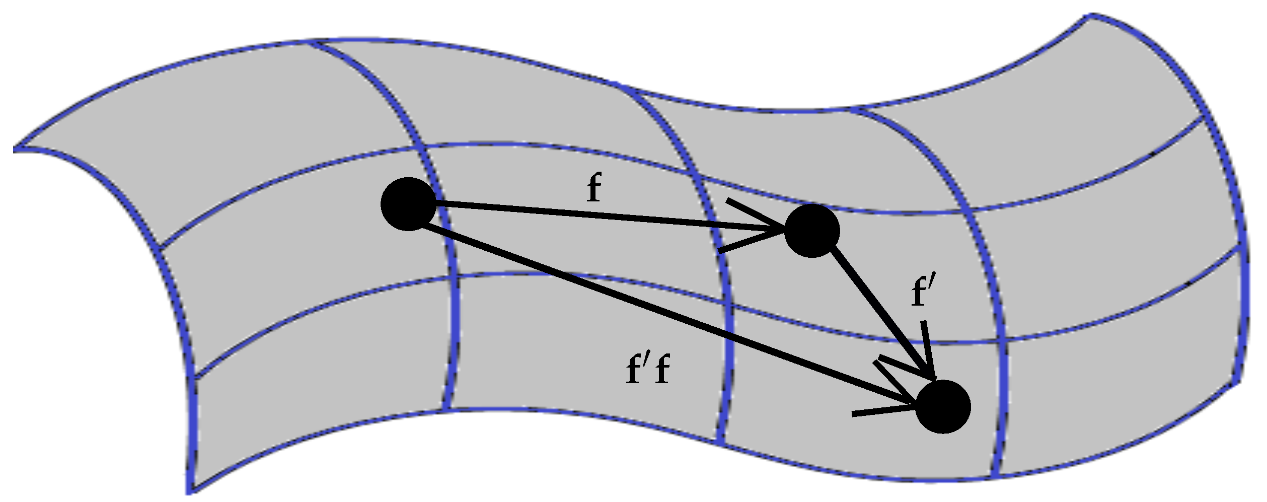
Figure 2.
Translation as a diffeomorphism on a Euclidean space.
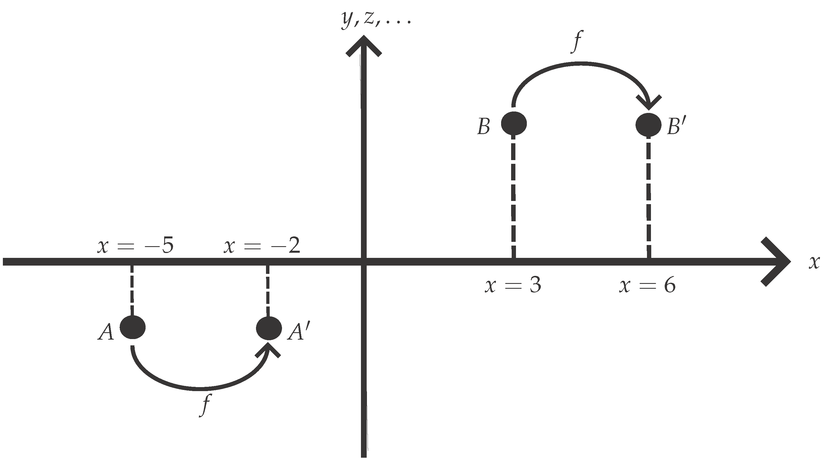
Figure 3.
Translation as a covariance on a Euclidean space.
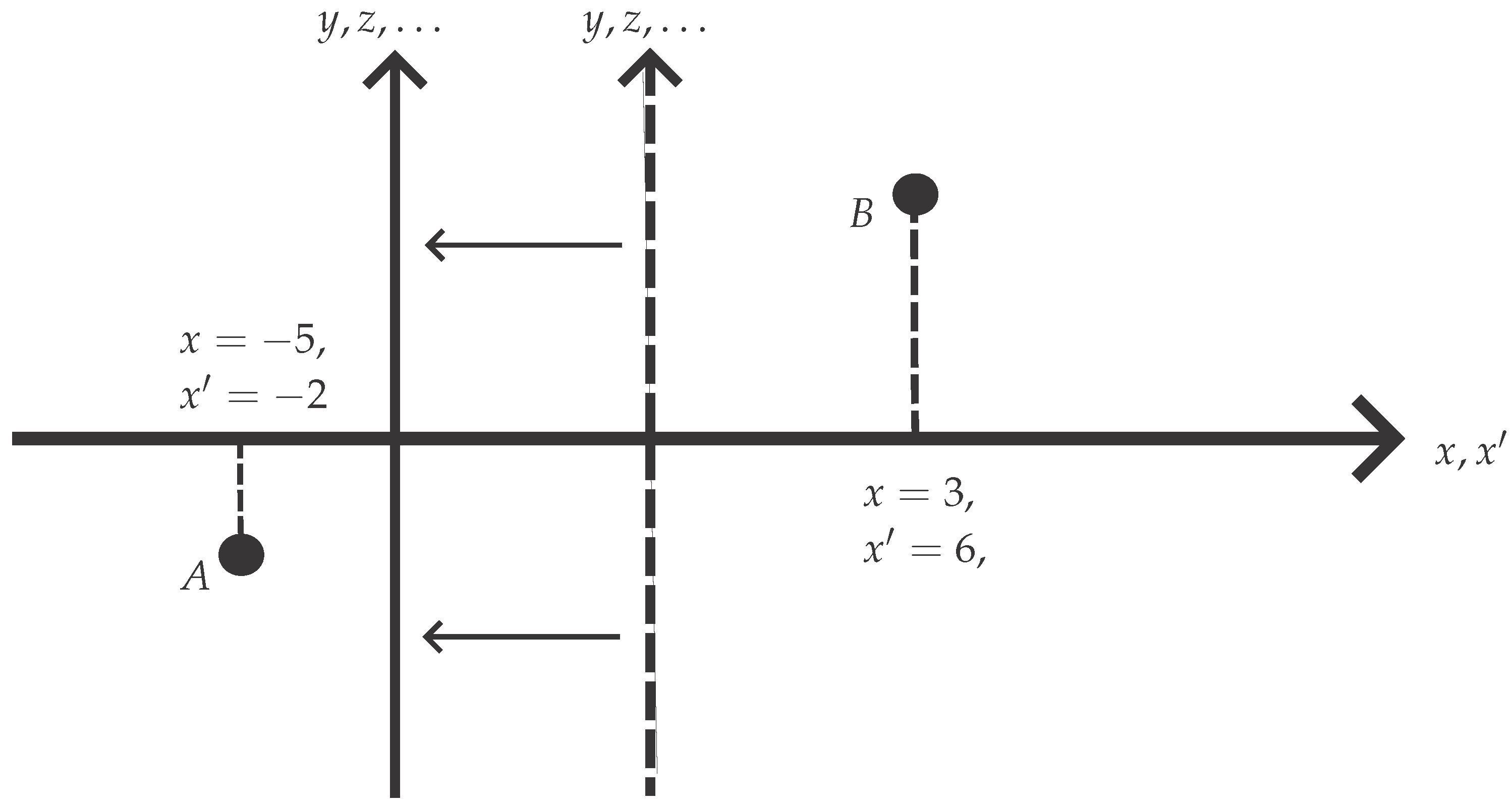
Figure 4.
Rotation as a diffeomorphism on a Euclidean space.
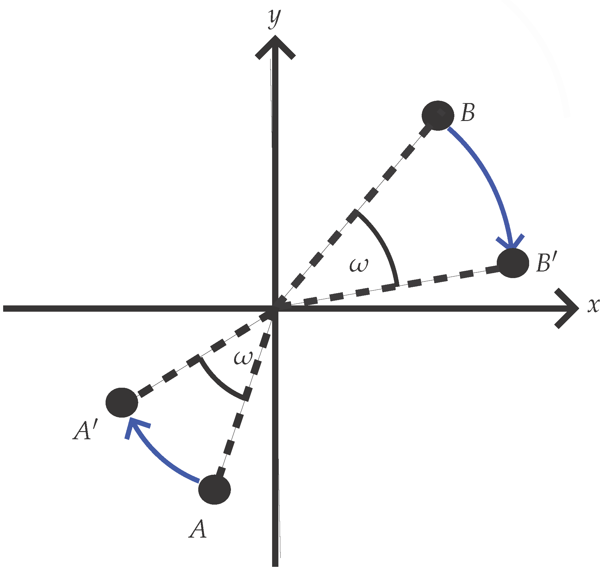
Figure 5.
Rotation as a covariance on a Euclidean space.
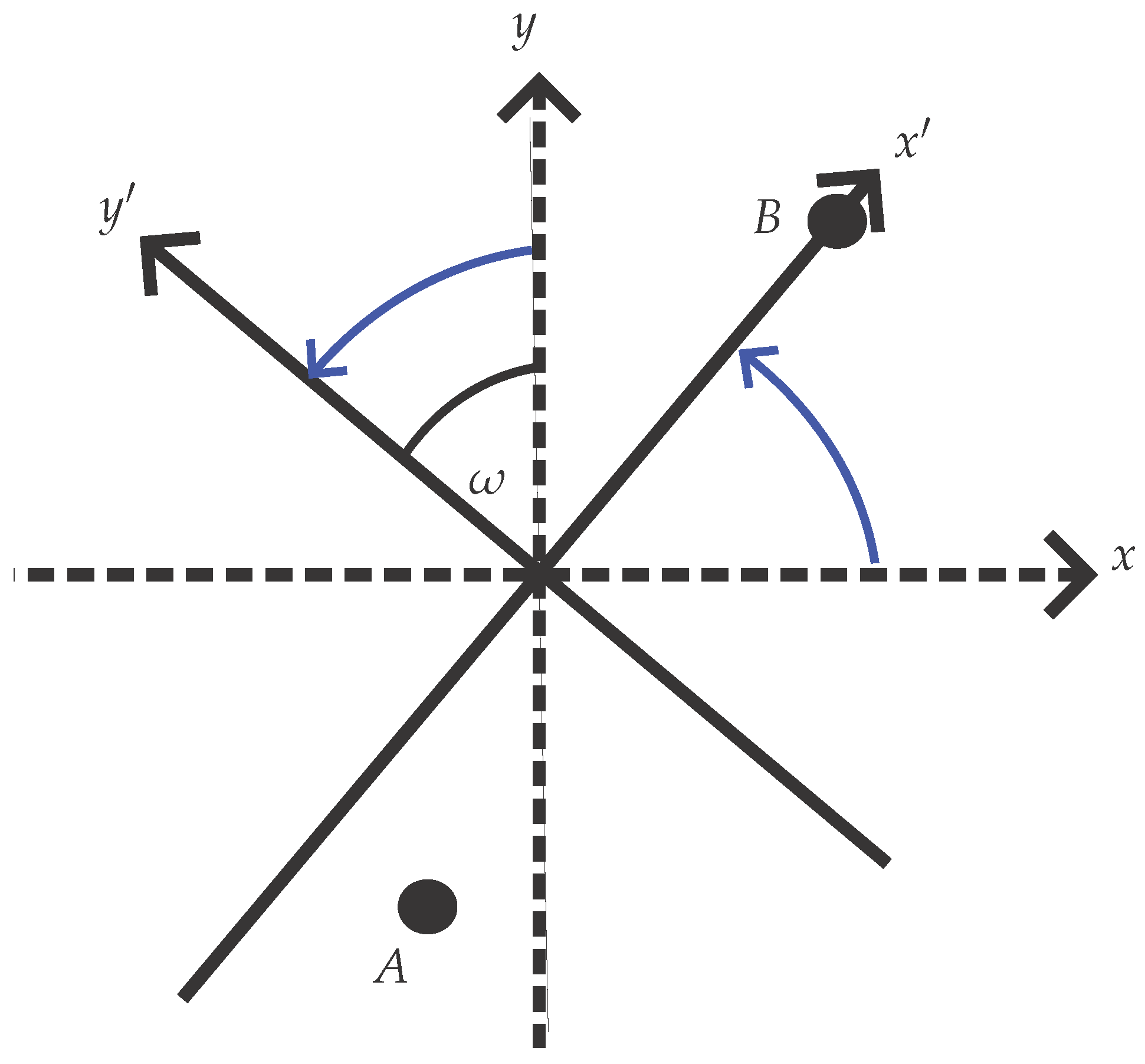
Figure 6.
Active translation of a vector field (dragging map).
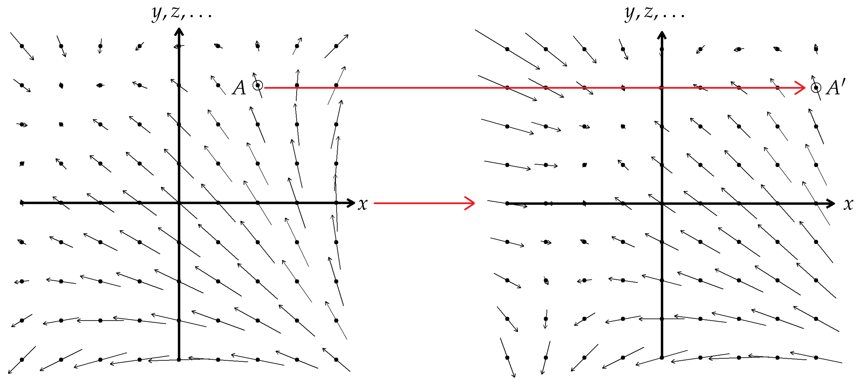
Figure 7.
Decomposition of a vector field at one point.

Figure 8.
Vector field with rotated coordinate system.
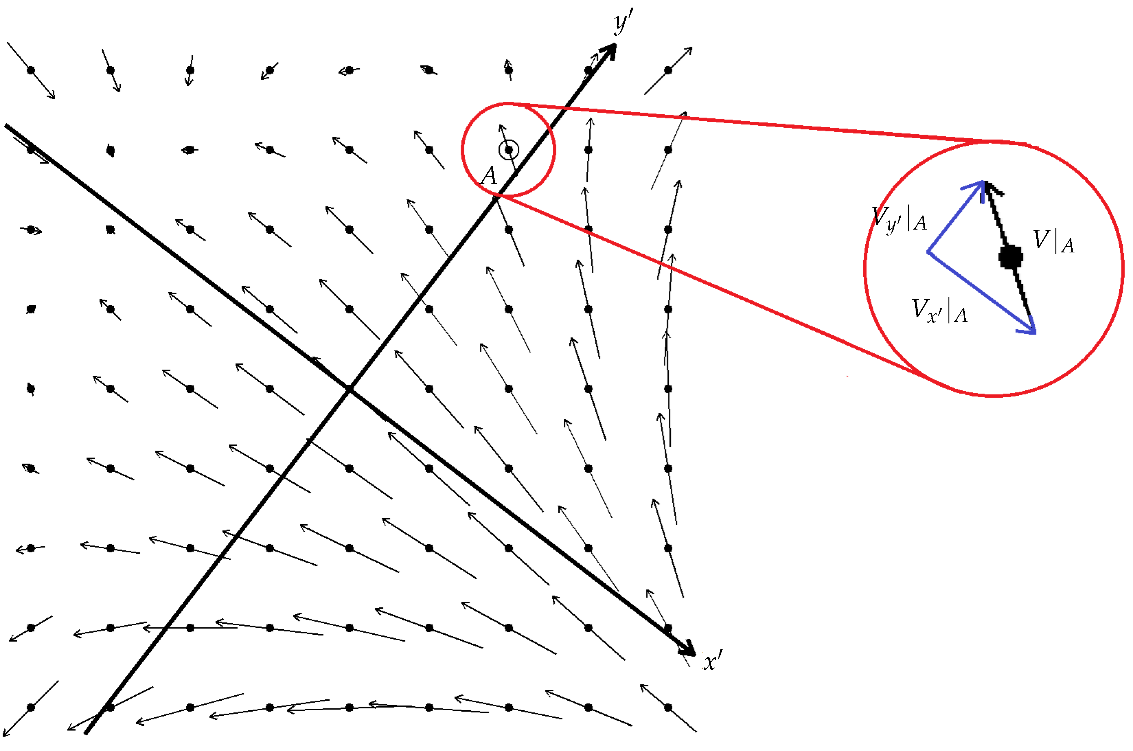
Figure 9.
Scalar field with discrete rotational symmetries.

Figure 10.
Scalar field with discrete translational symmetries.
Figure 11.
Vector field with rotational symmetries.
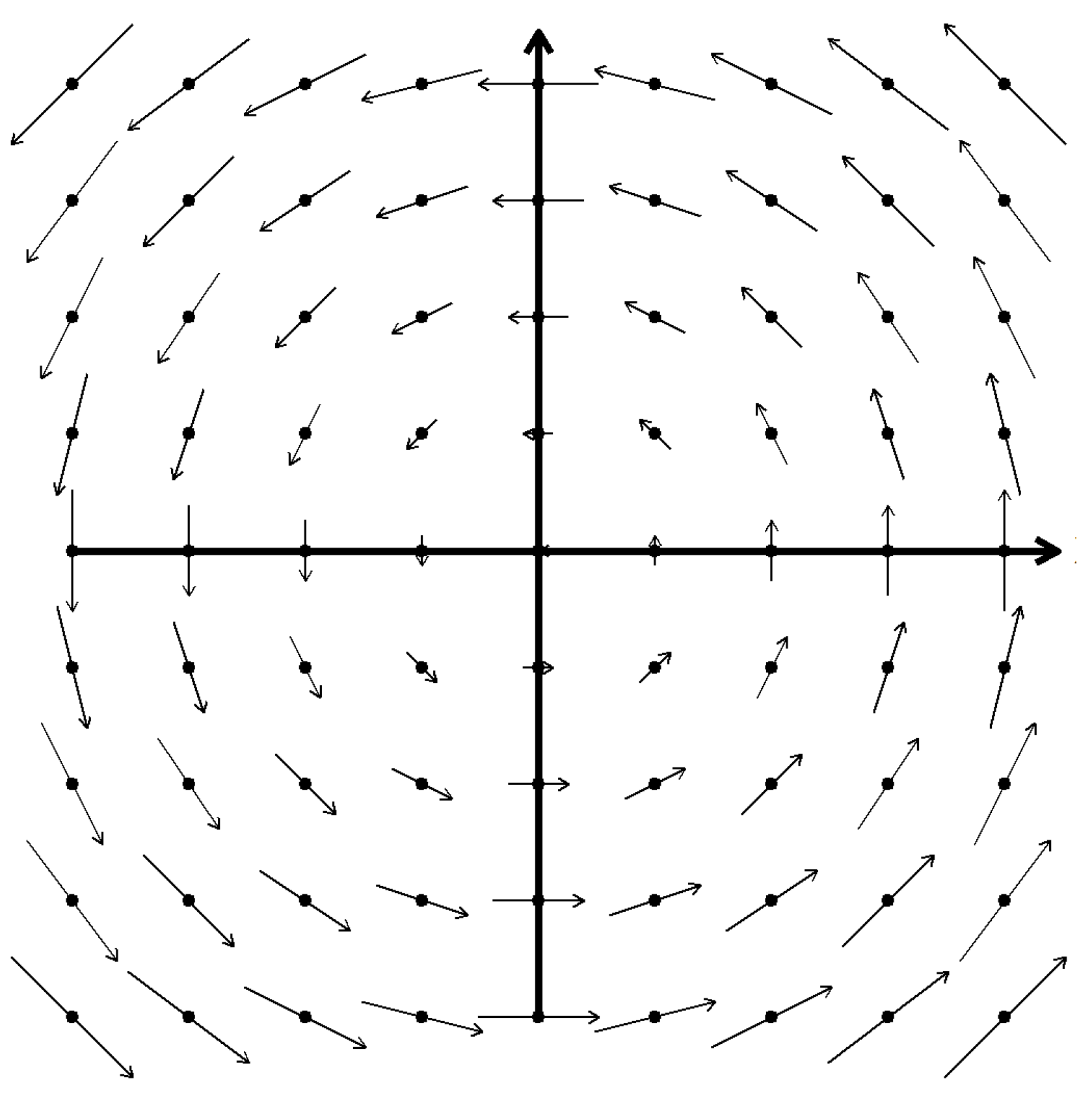
Figure 13.
Scalar field with continuous rotational symmetry.
Disclaimer/Publisher’s Note: The statements, opinions and data contained in all publications are solely those of the individual author(s) and contributor(s) and not of MDPI and/or the editor(s). MDPI and/or the editor(s) disclaim responsibility for any injury to people or property resulting from any ideas, methods, instructions or products referred to in the content. |
© 2025 by the authors. Licensee MDPI, Basel, Switzerland. This article is an open access article distributed under the terms and conditions of the Creative Commons Attribution (CC BY) license (http://creativecommons.org/licenses/by/4.0/).
Copyright: This open access article is published under a Creative Commons CC BY 4.0 license, which permit the free download, distribution, and reuse, provided that the author and preprint are cited in any reuse.


