
Submitted:
27 October 2025
Posted:
29 October 2025
You are already at the latest version
Abstract
Injectable Permeable Reactive Barriers (IPRBs) represent a promising in-situ technology for groundwater remediation, with sustainable adsorbents like biochar offering an alternative to activated carbon. This study optimized an IPRB process using a colloidal suspension of pinewood biochar stabilized with sodium carboxymethylcellulose (BC@CMC). The research first characterized the suspension stability under varying hydrochemical conditions, finding optimal colloidal stability at neutral to basic pH (6-9.4), while high ionic strength (>50 mM NaCl) and extreme pH values prompted aggregation. To enable effective delivery, pre-filtration through a 64-µm sieve was implemented, preventing column clogging and facilitating successful deep-bed distribution. The BC concentration was optimized to 3 g L⁻¹, maximizing injectable adsorbent mass. Batch adsorption tests demonstrated the biochar's high affinity for toluene (TOL) and tetrachloroethylene (PCE), with performance comparable to commercial activated carbon, particularly for PCE. The complete IPRB process was successfully validated through continuous-flow adsorption tests, where columns containing distributed BC@CMC showed high contaminant retention, with experimental retardation factors (Rₓ) of 144 ± 4 for TOL and 360 ± 6 for PCE. The study confirms that the optimized BC@CMC suspension enables highly efficient IPRB implementation, establishing this approach as a viable and sustainable strategy for field-scale groundwater remediation.
Keywords:
biochar-biopolymer composite
; colloidal biochar
; in-situ groundwater remediation
; injectable permeable reactive barriers (IPRB)
; contaminant adsorption
; contamination plume management
; petroleum hydrocarbons remediation
; chlorinated solvents remediation
; continuous-flow contaminants adsorption
; column breakthrough tests
1. Introduction
The pollution of groundwater represents a pressing worldwide challenge with significant implications for public health, ecological systems, and socioeconomic stability. As the primary source of potable water for nearly a third of the global populace, groundwater is indispensable, particularly in arid and semi-arid areas with limited surface water [1,2,3]. The integrity of this vital resource, however, is compromised by natural, geogenic processes like mineral dissolution and weathering, as well as by diverse anthropogenic activities such as agriculture, industrial operations, urban development, and inadequate waste disposal [2,4,5].
A wide array of contaminants (e.g., heavy metals, pesticides, fertilizers, organic solvents, and petroleum hydrocarbons) can be found in groundwater and can persist for decades or centuries before degrading naturally. The detection and remediation of these pollutants are often complicated by the fact that many are colorless and odorless [1,6,7]. The consequent human health impacts, which can include chronic illnesses and elevated cancer risks, are often severe and persistent [1,8,9]. Given the hidden nature of subsurface pollution and the complexity of aquifer environments, developing effective monitoring, prevention, and remediation strategies is an urgent priority to protect this essential resource for the future [1,3,4]. A major contributor to this problem is contamination by non-aqueous phase liquids (NAPLs), which are categorized as either light (LNAPLs, e.g., petroleum products) or dense (DNAPLs, e.g., chlorinated solvents) whose underground behavior is dictated by their density relative to water, immiscibility, and interactions with geological materials [10,11].
LNAPLs, being less dense than water, move downward through the unsaturated zone until they encounter the water table, where they tend to spread horizontally, forming lingering plumes. Their migration is heavily dependent on water table fluctuations, soil heterogeneity, and capillary forces, resulting in complex distribution patterns that complicate cleanup. For instance, the rate and extent of LNAPL movement are highly susceptible to changing water levels and the existence of preferential pathways in coarse soils, which can intensify local pollution [12,13,14]. Furthermore, factors like fluctuating water tables and temperature variations—intensified by climate change—can enhance LNAPL mobility and the leaching of toxic components into the aquifer, posing additional challenges for risk management and remediation [15,16]. In contrast, DNAPLs sink through the saturated zone due to their higher density, often penetrating deep into aquifers and pooling on low-permeability layers. Their persistence and low solubility make them long-lasting sources of contamination, as they gradually dissolve and create extensive dissolved plumes. The migration and transformation of DNAPLs are affected by the aquifer internal structure [11,[17]. Accurately modeling and monitoring their behavior is especially difficult because of their complex multiphase flow and the challenges of direct observation in the subsurface [10,11].
Over the past decades, a variety of remediation strategies have been developed to address NAPL-contaminated groundwater. The most common approaches include traditional pump-and-treat systems, in-situ chemical oxidation, soil vapor extraction, surfactant-enhanced flushing, and the use of permeable reactive barriers (PRBs) [18,19,20]. While pump-and-treat methods have been widely used, they are often energy-intensive, costly, and less effective for complete contaminant removal, especially in heterogeneous subsurface environments [18,19,21]. In-situ techniques, such as chemical oxidation and bioremediation, offer more sustainable alternatives but can be limited by reagent delivery and subsurface conditions [22,23,24]. Among these, permeable reactive barriers (PRBs) have emerged as a particularly promising and sustainable technology for in-situ groundwater remediation. PRBs are passive systems installed across the flow path of contaminated groundwater, where reactive materials intercept and treat contaminants as groundwater flows through the barrier [20,21,25]. The choice of reactive media—ranging from zero-valent iron (ZVI) and activated carbon to zeolites and biochar—enables PRBs to target a wide spectrum of contaminants, including NAPLs, heavy metals, and nutrients [26,27,28]. PRBs can be designed in various configurations (e.g., continuous trench, funnel-and-gate) and are valued for their low maintenance, long operational life, and minimal disturbance to the aquifer [20,25,29].
A significant advancement in PRB technology is the development of injectable permeable reactive barriers (IPRBs). Unlike traditional PRBs, which often require large-scale excavation, IPRBs involve the subsurface injection of reactive materials, such as nanoparticles, emulsions, or gels, directly into the contaminated zone [30,31,32]. This approach allows for targeted treatment of NAPL source zones, improved contact with contaminants, and applicability in challenging hydrogeological settings where conventional PRB installation is impractical [30,33,34]. Injectable PRBs can be tailored to enhance NAPL removal through mechanisms such as adsorption, chemical reduction, and bioremediation, and are increasingly being integrated with other remediation strategies for improved effectiveness [31,32,34]. IPRBs using colloidal activated carbon (CAC) have become a leading-edge technology for in situ groundwater remediation, particularly for persistent organic contaminants such as petroleum hydrocarbons and chlorinated solvents [35,36,37]. CAC is favored for its high surface area, strong adsorptive capacity, and ability to be distributed throughout the subsurface via injection, forming a reactive zone that immobilizes contaminants and prevents plume migration [38,39,40]. However, the successful deployment of CAC in groundwater systems hinges on achieving and maintaining colloidal stability, which is essential for effective subsurface transport and uniform barrier formation [41,42,43].
Our research aims to optimize an IPRB process based on the distribution of colloidal biochar (BC) into the aquifer as an environmentally sustainable alternative adsorbent to activated carbon (AC). BC is a carbon-rich, porous material produced by the thermal decomposition of biomass—such as wood, agricultural residues, or manure—under limited or no oxygen conditions, a process known as pyrolysis [44]. Its unique physicochemical properties, including high surface area, diverse surface functional groups, and customizable pore structure, make it an effective and sustainable adsorbent for environmental remediation applications [45,46]. In the groundwater remediation sector, biochar is increasingly used to remove a wide range of contaminants, including heavy metals, organic pollutants, and nutrients, through mechanisms such as adsorption, ion exchange and electrostatic attraction [44,45,47]. The performance of BC in contaminant removal is influenced by factors like feedstock type, pyrolysis temperature, and surface modification (engineered or modified biochars) often exhibiting enhanced sorption capacities [44,45,48]. Biochar can be applied directly to contaminated aquifers or used as a support for reactive materials (e.g., ZVI) to synergistically degrade or immobilize pollutants, offering a cost-effective, eco-friendly, and versatile solution for improving groundwater quality [49,50,51]. This study is a continuation of the research presented in Petrangeli Papini et al. [52], which focused on characterizing biochar@biopolymer composite suspensions for delivery into simulated aquifer columns. From those studies, a particularly promising composition emerged, with sodium carboxymethylcellulose (CMC) acting as a stabilizing agent for the biochar (BC@CMC).
Building upon these findings, the present work has a dual focus:
- The further characterization of the optimized BC@CMC suspension in aqueous environments under varying pH and ionic strength conditions to elucidate the influence of external parameters.
- The investigation of the delivery of the BC@CMC suspension as adsorbent within a simulated aquifer in a glass-beads packed column, followed by an evaluation of its adsorption capabilities through the continuous injection of synthetically contaminated water.
2. Materials and Methods
2.1. Production of Pinewood Biochar
Pine wood biochar (BC) derived from European pine was used as the raw material for the composite. This BC is a waste product from an industrial-scale biomass energy plant operated by Burkhardt Energy and Building Technology (Plößberg, Germany). The energy process involves a two-stage procedure: initial gasification of wood pellets at 950 °C (V3.90 unit), followed by syngas combustion in a combined heat and power (CHP) unit (CHP ECO 220). The BC used herein is thus a residual material from this cogeneration process, which is ordinarily destined for disposal.
2.2. Preparation of the BC@CMC Colloidal Suspensions
For the synthesis of the BC@CMC composites, biochar derived from pine wood and sodium carboxymethylcellulose (CMC 0.7 carboxymethyl groups per anhydroglucose unit; Merck Sigma-Aldrich, Milan, Italy) were used. The production protocol for the BC@CMC suspension had been previously optimized, with a specific focus on the stabilizer (CMC) concentration [52]. In the present work, the CMC concentration was fixed at the optimized value of 10 g·L⁻¹, while a range of higher BC concentrations—1, 2, 3, 4, and 5 g·L⁻¹—were investigated. A typical synthesis procedure was as follows: 10 g·L⁻¹ of CMC powder was mixed with the BC powder (previously sieved at 50 µm) in a weighing boat, and the solid mixture was mechanically homogenized with a spatula. This mixture was then added to the appropriate volume of distilled water produced with a Zeneer Power I Scholar-UV instrument (Full Tech Instruments, Rome, Italy). The suspension was stirred vigorously at room temperature until complete homogenization was achieved. This required approximately 2 hours for smaller volumes (up to a few hundred milliliters) and overnight for larger volumes (on the liter scale). Due to experimental evidence from preliminary studies (which will be discussed in the corresponding Results and Discussion section), it was necessary to perform pre-filtration of the BC@CMC suspension through sieves (with a mesh size between 50 and 64 µm) prior to its use in subsequent tests, in order to remove the larger BC aggregates.
2.3. Stability Tests: Effects of Ionic Strength and pH
Stability tests as a function of ionic strength (IS) and pHs were carried out in triplicate on BC 0.3 g·L⁻¹ @CMC 10 g·L⁻¹ suspension in distilled water. The IS was adjusted using NaCl solution to specific experimental values of 50, 100, 200, 300, 400 mM. The pH of the suspensions was carefully adjusted using small amounts of 0.1 M HCl or NaOH solutions in the 0.50-12 pH range. The suspensions were sonicated for 2 min, followed by stirring for 2 h. To evaluate the biochar sedimentation over time, the samples were monitored for changes in the absorbance value at 650 nm via UV-Vis, whereas the colloidal stability and hydrodynamic size (<2RH>, nm) evolution were measured by ζ-potential (ζ-pot., mV) and dynamic light scattering techniques, respectively.
2.4. Distribution Tests: Injection Simulation of BC@CMC in an IPRB
Column transport experiments were conducted to assess the deliverability and retention of the synthesized composites within a simulated aquifer. The experiments utilized transparent polymethylmethacrylate (PMMA) columns (14 cm in length × 2.5 cm in diameter) packed with glass beads (600–800 μm diameter) to simulate a porous medium representative of medium-grained sand.
The experimental setup operated as follows (Figure 1):
- The BC@CMC composite suspension was continuously fed from a magnetically stirred beaker using a Gilson Miniplus Evolution (Milan, Italy) peristaltic pump and injected into the column in an up-flow configuration to prevent air entrapment.
- The effluent from the column outlet was automatically collected into glass tubes by a fraction collector (Gilson 201-202) to facilitate monitoring.
The concentration of BC in the effluent was determined by measuring suspension turbidity at 650 nm using a photometer [52]. A specific calibration curve was established for each composite batch to ensure accurate quantification.
The tests were performed in two sequential phases:
- Distribution: Injection of the BC suspension to evaluate its transport through the porous medium.
- Elution: Subsequent flushing with ultra-pure water to elute weakly retained BC particles and quantify the fraction permanently retained by the column, thereby enabling a mass balance calculation.
The mass of BC retained within the column (mBC) was calculated according to the mass balance Equation (1):
where:
mBC = Σi (Qi ti C0 - Qi ti Ci)
- Qᵢ (L∙h-1) is the flow rate at the i-th time interval;
- ti (h) is the i-th time interval;
- C0 (g∙L-1) is the inlet BC concentration;
- Cᵢ (g∙L-1) is the effluent BC concentration at the i-th time interval.
To standardize the comparison of retention performance across different tests, the mass of BC retained per pore volume (PV) of BC@CMC fed (denoted as mPV) was calculated from the mass balance using Equation 2:
mPV = mBC / PV
The mass percentage fraction of BC retained on the column (fBC) relative to the dry mass of the porous medium (mGB) was also calculated via Equation 3:
fBC = 100 mBC / mGB
In a prior study [52], the same column setup was characterized through tracer tests, which yielded replicable results. Therefore, for the present experiments, the average values from that study were used to define the system hydraulic properties, including pore volume PV ((28 ± 2) mL) and effective porosity ε (0.41 ± 0.07).
BC transport tests were conducted at a flow rate of approximately Q of 0.6 mL·min-1, corresponding to an apparent velocity v of 0.3 cm·mim-1 and hydraulic retention time θ of 47 min. The results are presented as breakthrough curves, plotting the normalized effluent concentration (C/C₀) against the number of pore volumes eluted (PV).
2.5. Sedimentation Experiments on BC@CMC Suspensions
Sedimentation tests were conducted to evaluate the stability over time of BC@CMC suspensions at higher BC/CMC ratios than those investigated previously [52]. Specifically, the tests monitored sedimentation in the superficial layer (immediately below the suspension meniscus).
The procedure was as follows:
- The BC@CMC suspension was prepared as described in paragraph 2.2, maintaining a CMC concentration of 10 g L⁻¹ and varying the BC concentration between 1 and 5 g L⁻¹.
- 10 mL of the prepared suspension was placed into test tubes, and its stability was monitored through periodic sampling and photometric analysis.
Samples were always taken from the same depth (1 cm below the meniscus of the suspension) to ensure data reproducibility.
Equation 4 used to calculate the sedimentation in the superficial layer percentage at different time intervals (s) is as follows:
where:
s = 100 (af – ai) / ai
- af is the absorbance (BC concentration) at the investigated time;
- ai is the absorbance (BC concentration) at the start of the experiment.
2.6. Contaminant Adsorption Isotherms
Batch adsorption tests were conducted to evaluate the efficiency of raw BC in immobilizing trichloroethylene (TCE), tetrachloroethylene (PCE), and toluene (TOL) in a simulated aquifer medium. The BC used for the adsorption tests is the same as that used for the preparation of the BC@CMC suspensions, described in paragraph 2.1. The only pre-treatment before use was sieving at 50 µm.
The adsorption isotherms performed on the BC were replicated on a commercially available activated carbon (AC), Filtercarb PHA (Carbonitalia, Livorno, Italy), to evaluate the performance of the material under study against a standard adsorbent used in adsorption processes.
A 60 mg·L⁻¹ stock solution of the contaminants was prepared in a 1 L Tedlar bag (Supelco, Bellefonte, PA, USA) to prevent volatilization and headspace formation, by adding a volume of pure solvent (ACS ≥ 99.5%, Sigma-Aldrich, St. Louis, MO, USA). The solution was agitated on a horizontal shaker (ASAL Universal Table Shaker 709) for one week to ensure complete solubilization.
Batch experiments were performed in borosilicate glass vials (VWR International, Milan, Italy). A known mass of BC (ranging from 10 to 200 mg) was weighed into each reactor, which was then completely filled with approximately 0.02 L of the contaminated solution. The reactors were sealed with a Teflon butyl stopper (Wheaton, Millville, NJ, USA) and an aluminum cap, then mixed on a vertical rotating mixer (Biologix MX-RD-E, Camarillo, CA, USA) for 24 hours. Following mixing, the samples were allowed to be sedimented. An aliquot of the aqueous phase was subsequently withdrawn using a syringe for analysis. Each BC loading was performed in triplicate.
The concentration of the contaminant adsorbed onto the BC (SISO, mgCONT·gBC⁻¹) was calculated using Equation 5:
where C₀ is the initial contaminant concentration, C is the equilibrium liquid-phase concentration determined by gas chromatography, V is the volume of solution, and m is the mass of the adsorbent (BC or AC).
S = (C0V – CV) / m
The adsorption data were fitted with a Freundlich isotherm model (Equation 6) [53], which provided an optimal representation of the trend:
where:
S = KFCn
- S (mgCONT·gBC⁻¹) is the concentration of adsorbed contaminant on the BC;
- KF (Ln·gBC-1·mgCONT1-n) is Freundlich’s constant;
- C (mgCONT·L-1) is the equilibrium liquid-phase contaminant;
- n (dimensionless) is Freundlich’s exponent.
- The Freundlich constants KF and n were determined using SigmaPlot 12.0 software.
2.7. Continuous Flow Contaminant Adsorption on Distributed BC – IPRB Process Simulation
Continuous-flow adsorption column tests were conducted to validate the practical applicability of the proposed IPRB technology. The experimental procedure involved two main steps: first, a reactive adsorption zone (IPRB) was created within a packed column (simulating an aquifer) by distributing a BC@CMC suspension (paragraph 2.4). Second, a dilute aqueous solution of the contaminant (synthetic contaminated groundwater) was continuously injected into this pre-treated column. The experimental setup is depicted in Figure 2.
The synthetic groundwater feed, with a target contaminant concentration on the order of mg·L⁻¹, was prepared according to the procedure detailed in paragraph 2.6. To monitor the progression of the test, the effluent contaminant concentration was tracked via manual sampling and GC-FID analysis (paragraph 2.8). This sampling regimen allowed for the construction of the breakthrough curve, thereby enabling an assessment of the overall process effectiveness.
The mass of contaminant adsorbed within the column (mAD, mgCONT) was calculated according to the mass balance Equation (7):
where:
mAD = Σi (Qi ti C0,i - Qi ti Ci)
- Qᵢ (L∙h-1) is the flow rate at the i-th time interval;
- ti (h) is the i-th time interval;
- C0,i (g∙L-1) is the inlet contaminant concentration at the i-th time interval;
- Cᵢ (g∙L-1) is the effluent contminant concentration at the i-th time interval.
During the initial phase of column feeding, a reduced contaminant concentration was observed at the column inlet compared to the concentration in the storage bag (caused by adsorption phenomena onto the feeding tubing). Therefore, in Equation 6, the feed concentration is considered time-dependent.
The contaminant breakthrough curves were represented similarly to the BC distribution curves through graphical trends showing the ratio between the effluent concentration and the contaminant feed concentration (C/C₀) as a function of the pore volumes (PV) of contaminated synthetic groundwater. The data were subsequently fitted using Sigmaplot 12.0 software. The model used is that of the generalized logistic equation (Equation 8), typically employed to model adsorption processes in fixed-bed columns (also referred to as the Thomas, Bohart-Adams, or Yoon-Nelson model depending on the mechanistic approach) [54].
where:
C / C0 = 1 / {1 + exp [- a (PV – b)]}
- C₀ (mg∙L-1) is the average contaminant concentration in the column feed
- C (mg∙L-1) is the average contaminant concentration in the column discharge
- PV (dimensionless) is the number of pore volumes fed to the column
- a and b (dimensionless) model parameters
An additional parameter calculated from this test is the theoretical retardation factor Rt, a dimensionless number that describes how much slower a dissolved contaminant moves through groundwater than the groundwater itself. It was calculated from the values obtained from the Freundlich isotherm using the following Equation (9) [55]:
where:
Rt = 1 + (ρ / ε) KF n C0n-1
- ρ (g∙L-1) is the adsorbent bed density
- ε (dimensionless) is the bed porosity
- KF (Ln∙gn) is Freundlich’s constant
- C0 (g∙L-1) is the average column feed contaminant concentration
- n (dimensionless) is Freundlich’s exponent
Finally, the theoretically estimated retardation factor (Rt), based on values derived from the respective isotherms, was compared with the actual retardation factor calculated from the experimental data of the continuous adsorption test. The experimental retardation factor Rx (dimensionless) was estimated by inputting the data from the breakthrough curve in the mean residence time equation for a step-input curve (Equation 10) [56]:
where:
Rx = Σi {(PVi – PVi-1) [(1 - Ci-1 / C0,i-1) + (1 - Ci / C0,i)] / 2}
- C₀ (mg∙L-1) is the average contaminant concentration in the column feed
- C (mg∙L-1) is the average contaminant concentration in the column discharge
- PV (dimensionless) is the number of pore volumes fed to the column
2.8. Characterization Techniques and Analytical Methods
Ultraviolet-visible (UV–Vis) absorption spectra were acquired on a Varian Cary 100 spectrophotometer (Agilent Technologies, Milan, Italy), scanning the 200–900 nm wavelength range. All measurements were performed using 1 cm path length quartz cuvettes.
Turbidity of the column effluent during the BC composite distribution tests was monitored at 650 nm using a Shimadzu UV1800 UV–Vis-NIR (Milan, Italy) photometer equipped with 1 cm polystyrene cuvettes.
The pH was measured with an Eutech Instruments pH600 pH meter (Eutech Instruments Pte Ltd, Singapore), calibrated prior to use with standard buffer solutions at pH 4, 7, and 10.
The concentrations of tetrachloroethylene (PCE) and toluene (TOL) for both adsorption isotherm determination and continuous-flow adsorption experiments were quantified by gas chromatography. Analysis was performed using a TRACE 1600 gas chromatograph (Thermo Fisher Scientific, Monza, Italy) equipped with a flame ionization detector (FID) and a TriPlus 500 headspace autosampler. Separation was achieved on a TG-624 capillary column (30 m × 0.32 mm ID, 1.8 μm film thickness). The headspace autosampler was configured with an oven temperature of 80 °C, a transfer line temperature of 105 °C, and a soft shaking mode for 2 min. The GC method employed nitrogen as the carrier gas at a flow rate of 3.5 mL·min⁻¹. The injector and detector temperatures were maintained at 50 °C and 280 °C, respectively. The FID was supplied with hydrogen, air, and nitrogen at flows of 35, 350, and 40 mL·min⁻¹, respectively. The oven temperature program was as follows: hold at 50 °C for 2 min, ramp to 150 °C at 15 °C·min⁻¹, then ramp to 200 °C at 30 °C·min⁻¹, with a final hold at 200 °C for 3 min. Quantitative analysis was based on external calibration using aqueous standard solutions. Calibration curves for each analyte were constructed in the concentration range from 0.1 to 10 mg·L⁻¹ by serial dilution of stock solutions.
3. Results and Discussion
3.1. Stability Tests on BC@CMC Suspension
3.1.1. Effect of Ionic Strength
In order to investigate the influence of ionic strength on BC 0.3 g·L⁻¹ @CMC 10 g·L⁻¹ composite was prepared in the presence of different NaCl concentrations, from 50 mM up to 400 mM, and monitored via UV-Vis at 650 nm within 35 days of static aging (Figure 3). Compared with pristine BC@CMC composite, whose starting ionic strength was calculated to be 16 mM (due to 10 g·L⁻¹ of CMC matrix), the addition of NaCl at a concentration ≥ 50 mM resulted in a sharp decline in the %BC in suspension (calculated as A/A0) of about 70% after 5 days due to aggregation and settling phenomena. By day 7, all salt-treated samples drop to approximately 25-30%; then, sedimentation in the presence of the electrolyte tends to a plateau, stabilizing around 13-16% within a month. Interestingly, the aggregation and sedimentation of BC showed a concentration-independent behavior above 50 mM NaCl. This suggests that for this composite formulation, the presence of additional positively Na+ ions were able to neutralize the negative surface charge of –COO– of CMC (itself in the form of sodium salt, 0.7 degree of substitution), weakening the electrostatic repulsion responsible for the aqueous stability and dispersibility of the composite. Moreover, it has been reported that the addition of inert monovalent salts such as NaCl decreases the viscosity of CMC solutions, thus once the 50 mM of NaCl threshold was reached, further increases in salinity offer little additional impact on suspension stability [57]. It is worthy to note that the inherent stability of the composite in the presence of an electrolyte also strongly depends on the interfacial physicochemical properties of raw BC (which in turn depend on pyrolysis temperature and feedstock type, among others). Indeed, the presence of functional groups on BC surface drive the formation of electrostatic repulsion or steric stabilization effect with the polymer dispersing matrix [58]. In this case, the use of a BC pyrolyzed at 950°C resulted in highly disordered graphite-like domains and less residual functional groups with hydrogen bond-based interactions stabilizing the composite structure [52], thus making the composite more prone to aggregation at high electrolyte concentration.
3.1.2. Effect of pH
The effect of different pH values on the BC@CMC stability was studied in the pH range of 0.50-12, via the addition of small aliquots of HCl and NaOH 0.1 M. The spectrophotometric determination at 650 nm (Figure 4a), showed a destabilization of the composite at strong acidic (pH 0.50) and strong basic (pH 11-12) values. To a lesser extent, the influence of slightly acidic pHs was observed, with the native BC@CMC (without pH adjustment, i.e., pH 9.40) being the most stable at all time points.
Variations of average hydrodynamic particle diameters (<2RH>, evaluated by DLS analysis) and colloidal stability (expressed as ζ-potential value) over 40 days were also studied (Figure 4(b,c)). On freshly prepared suspensions, the size distribution fluctuates around 1000 nm in all cases, according to the presence of a large hydration shell physically stabilizing the biochar particles, as already studied [52] (Figure 4b). After 24 h and during the first 15 days, a general increase in the hydrodynamic size was found across all pH conditions, followed by stabilization or slight fluctuations over the remaining time. At pH 6.00 and 9.40 (native pH), particles exhibit the highest and most stable sizes, maintaining diameters close to or above 2000 nm. These values remain within the experimental error of the <2RH> measured for freshly prepared samples, indicating minimal size variation over time. Conversely, more extreme pH values, i.e., 0.50, 2.00, 11.00, and 12.00, resulted in a decrease in the particle size, with pH 2.00 and pH 11.00 showing the most significant reduction. The reduction was consistent with a sedimentation of dispersed BC over time, in agreement with UV-Vis studies (Figure 4a), thus resulting in the measurement of the remaining (small) colloidal fraction in suspension. These findings suggested that near-neutral or basic (native) environments represent the optimal pH window for the composite size stability.
A more detailed study of the pH influence on the composite aqueous stability was carried out by ζ-potential measurements (Figure 4c). At the acidic (pH 0.50-4.00) and highly basic media (pH 11.00, 12.00), the absolute |ζ-potential| values were significantly lower than intermediate pH values (6.00, 9.40), often falling below 30 mV, consistent with a higher propensity for BC particles aggregation (supporting observation from DLS measurements). At intermediate pH values, a ζ-potential exceeding 50 mV was observed, with native BC@CMC resulting in the most stable suspension (e.g., -50 ± 3 mV after 40 days), suggesting strong repulsive forces that prevent aggregation. The observed effects can be explained by considering the sodium CMC structure, an anionic, strongly charged polysaccharide with a pKa of ≃4.4 [59]. Lowering the pH below the pKa value leads to a protonation of negatively charged carboxylic groups, thereby reducing electrostatic repulsion (charge density) between polymer chains. This effect has been reported to decrease the CMC chain dimensions, reducing the viscosity and its long-term stability [60]. On the other hand, strong basic pHs due to NaOH addition are reported to decrease the charge density of the CMC, especially for low degree of substitution (≃ 0.7-0.8) which facilitates interchain associations and the solubilization of cellulose backbone initially stabilizing the encapsulated BC [56]. Overall, the data reveal a strong dependence of BC stability within the CMC matrix on the pH of the medium, confirming the superior properties of BC@CMC composite as prepared in its native conditions.
3.2. Distribution Tests: Injection Simulation of BC@CMC in an IPRB
The suspension distribution tests of BC@CMC within a packed column simulate the initial step of the investigated remediation process, i.e., the installation of a Permeable Reactive Barrier (PRB). This section presents the results of multiple distribution tests conducted with varying operational parameters to achieve progressive process optimization. The tests can be logically categorized as follows:
- Distribution of unfiltered BC@CMC (1-10 g·L⁻¹)
- Distribution of BC@CMC (1-10 g·L⁻¹) filtered at 50 μm
- Distribution of BC@CMC (1-10 g·L⁻¹) filtered at 64 μm
- Distribution of BC@CMC (3-10 g·L⁻¹) filtered at 64 μm
3.2.1. Distribution of Unfiltered BC@CMC (1-10 g·L⁻¹)
The distribution test was conducted according to the parameters specified in paragraph 2.4. This experiment represents a continuation of the research presented in Petrangeli Papini et al.[52] and was, therefore, performed using the BC@CMC composition optimized in the previous work, specifically a 1-10 g·L⁻¹ ratio.
As observed in the breakthrough curve (Figure 5), the initial elution profile aligns with established findings. The discharge of BC@CMC commences concurrently with the first pore volume (PV), exhibiting a concentration lower than the input solution (C/C0m = 0.64 ± 0.06). This provides initial evidence of BC retention via filtration processes within the porous matrix.
A more detailed analysis of the curve reveals two sharp, significant reductions in effluent concentration at approximately 11 and 14 PVs. These events were concomitant with an unintended, near-complete cessation of the column feed flow. The observed decrease in effluent concentration is attributed to the reduced fluid velocity, as this parameter is inversely proportional to colloids within a porous bed [61]. The flow rate reduction was due to a partial clogging of the system. This suggests a shift in the retention mechanism from deep-bed filtration to dominant surface filtration, leading to the formation of a filter cake on the inlet surface. This hypothesis will be further confirmed and discussed in the subsequent experiments (sub-paragraph 3.2.2).
The visual inspection of the column, as shown in Figure 6, provides further evidence of the retention mechanisms. The left image depicts a column saturated with deionized water (the wetting procedure before BC@CMC injection, as per paragraph 2.4), while the right picture shows the same column after the BC@CMC distribution test. A comparison of the bed coloration reveals a distinct greyish color in the post-test column, contrasting with the characteristic white of the clean glass beads. This color change is a clear indicator of BC retention via deep-bed filtration. However, Figure 6 also shows that the first centimeter of the bed is entirely black, with a sharp transition to the underlying greyish zone. This contrast indicates that surface filtration (or cake filtration) was the dominant retention mechanism [62].
3.2.2. Distribution of BC@CMC (1-10 g·L⁻¹) Filtered at 50 and 64 μm
Based on the results from sub-paragraph 3.2.1 and the formulated hypothesis that clogging is controlled by surface filtration, it is necessary to demonstrate the existence of a BC particle size fraction incapable of penetrating beyond the first centimeter of the filtering bed.
Given the known diameter of the collector (glass beads), the equivalent pore diameter can be estimated using the Kozeny-Carman equation [63], which in this case is approximately (320 ± 100) µm. Considering the presence of pore throats within the porous network, particles as large as one-third of the effective pore diameter are typically sufficient to cause blockage [64]. Consequently, particles with a higher diameter than 110 µm would be expected to rapidly clog the bed.
However, from the DLS analysis on BC@CMC suspension showed a single population centered at <2RH> = (1100 ± 290) nm existing as colloidal fraction (Figure 4b), significantly smaller than the predicted clogging size.
This apparent discrepancy can be explained by the intrinsic limitation of the DLS instrument, which is not able to detect particles above 10 µm. It is, therefore, plausible that populations of larger BC aggregates exist in the suspension. These aggregates may form in aqueous environments but remain stabilized in suspension by the CMC, preventing their sedimentation [65]. Such aggregates would be the primary agents responsible for the observed surface filtration and rapid clogging.
To verify the aforementioned hypothesis, the BC@CMC suspension was filtered using sieves with mesh sizes of 50 and 64 µm to potentially remove large aggregates. The effect of this pre-filtration on the transport of the suspension through the column was then evaluated.
As shown in Figure 7a, a significant fraction of the BC@CMC was retained on the sieves after the filtration of 2 L of suspension, though it constituted a distinct minority of the total mass. This residue provides direct evidence for the existence of the large, clogging-prone particle fraction hypothesized in the previous section. The presence of this retained fraction confirms that a population of particles exceeding tens of micrometers in size exists within the stabilized suspension. Further DLS analysis, carried out on BC@CMC sieved at 50 and 64 µm, is presented in Figure 7b. Compared with pristine BC@CMC, the filtering procedure also slightly reduced the size of the BC colloidal fraction, whose hydrodynamic size followed the order pristine > 64 µm > 50 µm, as expected. The overall size decreased from (1100 ± 290) nm (pristine), to (1040 ± 195) nm (filtered at 64 µm), and (915 ± 180 nm) (filtered at 50 µm), also narrowing the polydispersity of the samples. However, in all cases, optimal colloidal stability was maintained, ranging from (-60 ± 2) mV for the untreated composite to (-51 ± 2) mV and (-52 ± 2) mV, after filtration at 64 and 50 µm, respectively.
Figure 8a presents the breakthrough curves from three distribution tests: one pre-filtered through a 50 µm sieve and two through a 64 µm sieve, all including the subsequent water flushing phase. The regularity of these curves indicates the absence of clogging events, thereby confirming the hypothesis that the presence of a coarse BC aggregate fraction is responsible for the rapid column clogging observed in non-pre-filtered tests.
A clear distinction is also evident between the curves. Specifically, the normalized effluent concentrations (C/C₀) during the loading phase for the F64 tests are significantly lower (0.57 ± 0.05) than those for the F50 test (0.9 ± 0.2). This logically corresponds to higher particle retention within the column for the F64 suspension.
Based on these observations, it can be concluded that, under our specific operational conditions, the BC particle fraction between 50 and 64 µm is responsible for a significant portion of the retention. Consequently, pre-filtration is a useful process to prevent surface clogging; however, excessive pre-filtration, as demonstrated by the F50 condition, introduces system inefficiency. While it successfully prevents clogging, it also leads to a deeper and more gradual retention of particles, necessitating a greater number of pore volumes to elute the same mass of BC compared to the F64 case (Figure 8b).
Starting from the mass balance Equation (5), several parameters were calculated to evaluate the effectiveness of the BC@CMC distribution process. The calculated parameters were: the distributed BC mass (mBC), the distributed BC mass per injected pore volume (mPV), and the mass percentage of BC per dry mass of porous medium (fBC). The aforementioned parameters are reported in Table 1.
By examining the mBC data, it is clear that the distributed mass in the F64 tests is significantly higher than that in the F50 tests. As previously emphasized, this indicates that a significant amount of BC capable of being retained by the columns under the studied experimental conditions is present within the narrow grain size range between 50 and 64 μm. Also, by looking at the fBC data, we can observe that these values reflect the trends of mBC and mPV. The fBC values for the F64 tests fall within the center of the typical operational range (0.02 - 0.8%) for adsorbent distribution in aquifers [66,67,68].
3.2.3. Distribution of BC@CMC (3-10 g/L) Filtered at 64 μm
Based on suspension stability tests that will be illustrated later (paragraph 3.3), it was decided to evaluate the possibility of distributing a more concentrated BC suspension: by working at higher BC concentrations, it is possible to distribute a greater mass of adsorbent with a reduced suspension volume, offering significant operational advantages from the perspective of future field applications.
The stability tests revealed that it is possible to triple the BC concentration while maintaining the same CMC concentration and maintaining the suspension stability almost unchanged. Considering this, a distribution test was conducted with a BC@CMC suspension at a concentration of 3-10 g∙L⁻¹ (BC3), also filtered through a 64 μm sieve.
Observing the graph in Figure 9, it is possible to appreciate the overall trend of the distribution test (BC3). In particular, it can be noted that phase L lasts about one-third (≈ 10 PV) compared to the tests with BC 1 g∙L⁻¹ (BC1). This is intentional, as the aim was to keep the accumulated masses in the column nearly constant to ensure comparability with the BC1 tests in terms of mBC and fBC. Further observation of the graph shows that in this case, the plateau in terms of C/C0m is at a higher value compared to the BC1-F64 tests (0.70 ± 0.05 vs. 0.57 ± 0.05). The lower retention in this case could be due to the higher concentration, as trends of this kind have been documented in the literature [69,70]. Despite the lower retention efficiency of the column, the distributed mass per pore volume in BC3-F64 was significantly higher (mPV 25 ± 3 mg) than in BC1-F64 (mPV 9.9 ± 0.7 mg). The mBC settled at a value of (220 ± 10) mg and an fBC of (0.22 ± 0.04)%, thus in line with the BC1 tests.
3.3. Sedimentation Tests to Verify High Concentration BC@CMC Stability
To assess the possibility of increasing the BC concentration at a constant CMC in the suspensions to be distributed while maintaining system stability, sedimentation tests of the superficial layer were conducted. As described in the experimental protocol in paragraph 2.5, the variation in BC concentration at 1 cm from the liquid meniscus was monitored over time.
This approach was chosen because, when working with a colloidal suspension characterized by high particle polydispersity, sedimentation over time leads to the formation of a concentration gradient with increasing depth. This is due to the establishment of a sedimentation-diffusion stratification phenomenon, typical of such systems [71,72,73].
In our case, this phenomenon can be observed in a test tube from the experiment under examination, which has reached a dynamic equilibrium (Figure 10a). Two distinct portions are visible: a clearer upper portion and a darker lower one—likely representative of the two particle populations present in the system (the former corresponding to the micron-sized particles detected by DLS, and the latter to the residual tens-of-micron-sized particles from the 64 µm sieve filtration process).
As per Table 2, five progressive increments of 1 g L⁻¹ in BC concentration relative to the starting suspension were investigated in triplicate. Daily samplings of the superficial layer were performed to monitor the trend of the surface concentration over time relative to the initial concentration. Monitoring continued until the values stabilized at 96 hours of quiescence.
It can be observed that the values for concentrations between 1 and 3 g L⁻¹ of BC are virtually overlapping, distinctly separate from the values of the 4 and 5 g L⁻¹ samples. The former was averaged and are reported in the graph in Figure 10b, where the difference in behavior can be appreciated.
Based on these findings, to optimize the distribution process in a porous medium while maintaining suspension properties similar to those previously investigated, it was decided to conduct distribution tests with suspensions containing up to 3 g L⁻¹ of BC.
3.4. Contaminant Adsorption Isotherms on BC and AC
To evaluate the actual adsorption capacities of the BC, batch adsorption isotherms were conducted using the protocol detailed in paragraph 2.6. The isotherms were performed on two model contaminants belonging to the most common organic contaminant classes: toluene (TOL) as a representative of petroleum hydrocarbons and perchloroethylene (PCE) as a representative of chlorinated solvents. The Freundlich equation fitting results are summarized in Table 3. This equation was chosen for the fitting after tests with other equations, which returned larger errors for the parameters.
The KF and n parameters indicate the affinity between the contaminant and the adsorbent. A higher KF means that, for the same contaminant mass at equilibrium, more will be distributed onto the adsorbent and less will remain in the water. The parameter n describes how this affinity changes with the contaminant concentration; typically, n < 1 indicates that the affinity decreases as the equilibrium concentration increases.
Based on the parameters in Table 3 and the trends shown in Figure 11(a,b), it can be stated that the investigated BC is a valid alternative adsorbent to AC, as the KF values are of the same order of magnitude. In particular, for PCE, the adsorption capacities can be observed to be nearly overlapping.
The Freundlich parameters characterizing the adsorption capacity of the BC for the different contaminants will be used to estimate the theoretical retardation factors (Rt) in the continuous adsorption tests and will be compared with the experimentally measured retardation factors (Rx).
3.5. Continuous Flow Contaminant Adsorption on Distributed BC – IPRB Process Simulation
Herein, the results of continuous-flow adsorption tests of contaminants on columns packed with BC, using the BC@CMC distribution processes analyzed in paragraph 3.2 are reported. These tests represent the final step in validating and verifying the efficiency of the IPRB. Following the BC@CMC distribution process, the tests aim to confirm its actual capacity to sequester the contaminant from the aqueous phase, thereby delaying the advance of the contaminant plume front.
In line with the results presented in the previous paragraphs, continuous-flow adsorption tests were performed using the contaminants investigated via batch adsorption isotherms—namely, TOL and PCE (paragraph 3.3)—on columns F-64-1 and F-64-2, respectively. The breakthrough curves are shown in Figure 12. By comparing the curves, it can be observed that TOL breaks through significantly faster than PCE, despite their measured BC masses (mBC) being nearly identical (300 ± 10 and 320 ± 10, respectively). This finding is consistent with the greater affinity of PCE compared to TOL, as indicated by the KF values estimated from the isotherms (57 ± 4 and 30 ± 2, respectively).
The theoretical retardation factors (Rt), calculated based on the Freundlich isotherm parameters and the specific column properties, were (56 ± 5) for TOL and (190 ± 20) for PCE. Although the ratio between these theoretical values is consistent with the experimental results, their absolute values are significantly lower than the experimental retardation factors (Rx), which were (144 ± 4) for TOL and (360 ± 6) for PCE.
The discrepancy between the Rt and Rx values, while not particularly large, is nevertheless significant and systematic. This indicates that the isotherms likely underestimate the actual adsorption capacity of the biochar (BC) once it is distributed within a column.
The BC used for the isotherm tests was raw (not stabilized with CMC). Consequently, regardless of its initial particle size, raw BC in water tends to aggregate rapidly, forming large clusters (even up to millimeter size). This reduces its exposed surface area to the surrounding environment and, thus, the area available for adsorption [52].
In the distribution tests, however, the BC is stabilized by CMC, which prevents its aggregation. It is important to note that during the column flushing with water, the CMC is inevitably removed due to its high solubility in water. This could allow for some re-aggregation of adjacent BC particles. However, because the BC is retained in the porous medium by adhesion or straining, the extent of aggregation will remain limited [74]. Therefore, even though the BC in the column during the adsorption phase is devoid of stabilizer, its available surface area for adsorption will still be greater than that of the BC used in the batch isotherms, as in the latter case, there was nothing to prevent BC aggregation. In any case, both the Rt and Rx values allow for the installation of an efficient IPRB. Assuming a field application under realistic conditions – with a 3 m barrier [65] in a medium sand aquifer (K = 10⁻⁴ m·s-1) and a hydraulic gradient of 0.005 m·m-1, resulting in a seepage velocity of 4 cm/day – the calculated barrier breakthrough times are 27 years for TOL and 82 years for PCE. These figures are consistent with those of field-implemented barriers, especially when considering that the plume concentrations simulated in this work (over 3 orders of magnitude above regulatory limits) are inversely proportional to Rt (Equation 9).
4. Conclusions
This work further optimized the process for producing and distributing a BC@CMC suspension within a simulated column aquifer, validating its applicability in IPRB process. The entire process was also verified through continuous adsorption column tests using BC-packed columns via BC@CMC distribution. The characterization of the BC@CMC suspension was conducted by varying pH and ionic strength (IS), as these are parameters that can influence its colloidal stability. A rapid destabilization occurred at NaCl concentrations above 50 mM, likely due to charge neutralization and reduced electrostatic repulsion. Likewise, extreme pH values (≤2 and ≥11) promoted sedimentation, while intermediate pH conditions (pH 6-9.40) preserved suspension stability through stronger surface charge repulsion, as confirmed by ζ-potential and DLS analyses.
Regarding the optimization of the BC@CMC suspension distribution, the work initially focused on preventing early clogging phenomena caused by superficial filtration/retention in the initial portion of the bed, and subsequently on maximizing the distributable adsorbent mass per volume of injected suspension.
The solution to the clogging issues was to pre-filter the BC@CMC suspension upstream of the column injection using a 64 µm sieve; this approach removed the larger aggregates that could rapidly clog the pores a few centimeters from the injection point.
On the other hand, concerning the maximization of working concentrations, efforts were focused on increasing the BC concentration while keeping the CMC concentration constant. In this case, sedimentation tests showed that the same hydrodynamic properties of the BC@CMC suspension could be maintained at BC concentrations up to 3 g∙L⁻¹, with CMC kept at 10 g∙L⁻¹. Following these optimizations, it was possible to load the columns with an mBC of (220 ± 10) mg, corresponding to an fBC of (0.22 ± 0.04)%, in approximately 10 PVs of injection. This outcome aligns with the requirements for an adsorbent bed that ensures adsorption effectiveness without significant reductions in permeability.
Before simulating the IPRB process, batch adsorption isotherms were conducted for the model contaminants TOL and PCE to evaluate the adsorption capacities of the BC and a commercial AC. These measurements revealed that the adsorption capacities of BC are not only comparable to those of AC but are even nearly identical in the case of PCE.
The actual simulation of the IPRB process was finalized with continuous adsorption column tests. The columns were packed with BC via the BC@CMC distribution process, and the results demonstrated that this system delays the contaminant breakthrough front by 2 orders of magnitude for TOL (Rx = 144 ± 4) and by 3 orders of magnitude for PCE (Rx = 360 ± 6). Overall, these values confirm the BC@CMC's suitability for use in IPRBs for groundwater remediation.
Author Contributions
Conceptualization, supervision, funding acquisition, writing - review & editing, M.P.P. and I.F.; methodology, investigation, visualization, writing - original draft, D.F. and S.C. All authors have read and agreed to the published version of the manuscript.
Funding
This research was partially funded by Sapienza Ateneo Ricerca 2024, grant number RM124190F0042AFB.
Data Availability Statement
The raw data supporting the conclusions of this article will be made available by the authors on request.
Conflicts of Interest
The authors declare no conflicts of interest.
Abbreviations
The following abbreviations are used in this manuscript:
| AC | Activated Carbon |
| BC | Biochar |
| BC1 | Biochar 1 g∙L-1 |
| BC3 | Biochar 3 g∙L-1 |
| CAC | Colloidal Activated Carbon |
| CMC | Sodium Carboxymethylcellulose |
| DLS | Dynamic Light Scattering |
| GC-FID | Gas Chromatography – Flame Ionization Detector |
| IS | Ionic Strength |
| IPRB | Injectable Permeable Reactive Barrier |
| DNAPL | Dense Non-Aqueous Phase Liquids |
| LNAPL | Light Non-Aqueous Phase Liquids |
| NAPL | Non-Aqueous Phase Liquids |
| PCE | Perchloroethylene |
| PRB | Permeable Reactive Barrier |
| PMMA | Polymethylmethacrylate |
| PV | Pore Volume |
| TOL | Toluene |
| UV-Vis-NIR | Ultraviolet – Visible – Near InfraRed |
References
- Ravindiran, G.; Rajamanickam, S.; Sivarethinamohan, S.; Karupaiya Sathaiah, B.; Ravindran, G.; Muniasamy, S.K.; Hayder, G. A Review of the Status, Effects, Prevention, and Remediation of Groundwater Contamination for Sustainable Environment. Water 2023, 15, 3662. [Google Scholar] [CrossRef]
- Ullah, Z.; Rashid, A.; Ghani, J.; Nawab, J.; Zeng, X.-C.; Shah, M.; Alrefaei, A.F.; Kamel, M.; Aleya, L.; Abdel-Daim, M.M.; et al. Groundwater Contamination through Potentially Harmful Metals and Its Implications in Groundwater Management. Front. Environ. Sci. 2022, 10, 1021596. [Google Scholar] [CrossRef]
- Karunanidhi, D.; Subramani, T.; Srinivasamoorthy, K.; Yang, Q. Environmental Chemistry, Toxicity and Health Risk Assessment of Groundwater: Environmental Persistence and Management Strategies. Environmental Research 2022, 214, 113884. [Google Scholar] [CrossRef]
- Li, P.; Karunanidhi, D.; Subramani, T.; Srinivasamoorthy, K. Sources and Consequences of Groundwater Contamination. Arch Environ. Contam. Toxicol. 2021, 80, 1–10. [Google Scholar] [CrossRef]
- Chandnani, G.; Gandhi, P.; Kanpariya, D.; Parikh, D.; Shah, M. A Comprehensive Analysis of Contaminated Groundwater: Special Emphasis on Nature-Ecosystem and Socio-Economic Impacts. Groundwater for Sustainable Development 2022, 19, 100813. [Google Scholar] [CrossRef]
- Abanyie, S.K.; Apea, O.B.; Abagale, S.A.; Amuah, E.E.Y.; Sunkari, E.D. Sources and Factors Influencing Groundwater Quality and Associated Health Implications: A Review. Emerging Contaminants 2023, 9, 100207. [Google Scholar] [CrossRef]
- Kurwadkar, S. Occurrence and Distribution of Organic and Inorganic Pollutants in Groundwater. Water Environment Research 2019, 91, 1001–1008. [Google Scholar] [CrossRef]
- Yang, X.; Du, J.; Jia, C.; Yang, T.; Shao, S. Groundwater Pollution Risk, Health Effects and Sustainable Management of Halocarbons in Typical Industrial Parks. Environmental Research 2024, 250, 118422. [Google Scholar] [CrossRef] [PubMed]
- Wu, J.; Sun, Z. Evaluation of Shallow Groundwater Contamination and Associated Human Health Risk in an Alluvial Plain Impacted by Agricultural and Industrial Activities, Mid-West China. Expo Health 2016, 8, 311–329. [Google Scholar] [CrossRef]
- Sethi, R.; Di Molfetta, A. Transport of Immiscible Fluids. In Groundwater Engineering; Springer Tracts in Civil Engineering; Springer International Publishing: Cham, 2019; ISBN 978-3-030-20514-0. [Google Scholar]
- Ju, M.; Li, X.; Wu, R.; Xu, Z.; Yin, H. Research Hotspots and Trend Analysis in Modeling Groundwater Dense Nonaqueous Phase Liquid Contamination Based on Bibliometrics. Water 2024, 16, 2840. [Google Scholar] [CrossRef]
- Suo, K.; Zhao, M.; Liu, Y.; Liu, H.; Jia, M. A Study on the Monitoring of LNAPL Migration Using ERT. PLoS ONE 2025, 20, e0315624. [Google Scholar] [CrossRef]
- Almaliki, D.F.; Ramli, H.; Zaiter, A. Experimental Investigation of Single and Intermittent Light Non-Aqueous Phase Liquid Spills Under Dynamic Groundwater. Civ Eng J 2025, 11, 290–307. [Google Scholar] [CrossRef]
- Waqar, A. Evaluation of Factors Causing Lateral Migration of Light Non-Aqueous Phase Liquids (LNAPLs) in Onshore Oil Spill Accidents. Environ Sci Pollut Res 2024, 31, 10853–10873. [Google Scholar] [CrossRef] [PubMed]
- Cavelan, A.; Golfier, F.; Colombano, S.; Davarzani, H.; Deparis, J.; Faure, P. A Critical Review of the Influence of Groundwater Level Fluctuations and Temperature on LNAPL Contaminations in the Context of Climate Change. Science of The Total Environment 2022, 806, 150412. [Google Scholar] [CrossRef] [PubMed]
- Cavelan, A.; Faure, P.; Lorgeoux, C.; Colombano, S.; Deparis, J.; Davarzani, D.; Enjelvin, N.; Oltean, C.; Tinet, A.-J.; Domptail, F.; et al. An Experimental Multi-Method Approach to Better Characterize the LNAPL Fate in Soil under Fluctuating Groundwater Levels. Journal of Contaminant Hydrology 2024, 262, 104319. [Google Scholar] [CrossRef]
- Shi, J.; Chen, X.; Ye, B.; Wang, Z.; Sun, Y.; Wu, J.; Guo, H. A Comparative Study of DNAPL Migration and Transformation in Confined and Unconfined Groundwater Systems. Water Research 2023, 245, 120649. [Google Scholar] [CrossRef]
- Budania, R.; Dangayach, S. A Comprehensive Review on Permeable Reactive Barrier for the Remediation of Groundwater Contamination. Journal of Environmental Management 2023, 332, 117343. [Google Scholar] [CrossRef]
- Lawrinenko, M.; Kurwadkar, S.; Wilkin, R.T. Long-Term Performance Evaluation of Zero-Valent Iron Amended Permeable Reactive Barriers for Groundwater Remediation – A Mechanistic Approach. Geoscience Frontiers 2023, 14, 101494. [Google Scholar] [CrossRef] [PubMed]
- Obiri-Nyarko, F.; Grajales-Mesa, S.J.; Malina, G. An Overview of Permeable Reactive Barriers for in Situ Sustainable Groundwater Remediation. Chemosphere 2014, 111, 243–259. [Google Scholar] [CrossRef]
- Faisal, A.A.H.; Sulaymon, A.H.; Khaliefa, Q.M. A Review of Permeable Reactive Barrier as Passive Sustainable Technology for Groundwater Remediation. Int. J. Environ. Sci. Technol. 2018, 15, 1123–1138. [Google Scholar] [CrossRef]
- Ciampi, P.; Cassiani, G.; Deidda, G.P.; Esposito, C.; Rizzetto, P.; Pizzi, A.; Papini, M.P. Understanding the Dynamics of Enhanced Light Non-Aqueous Phase Liquids (LNAPL) Remediation at a Polluted Site: Insights from Hydrogeophysical Findings and Chemical Evidence. Science of The Total Environment 2024, 932, 172934. [Google Scholar] [CrossRef]
- Liu, J.-W.; Wei, K.-H.; Xu, S.-W.; Cui, J.; Ma, J.; Xiao, X.-L.; Xi, B.-D.; He, X.-S. Surfactant-Enhanced Remediation of Oil-Contaminated Soil and Groundwater: A Review. Science of The Total Environment 2021, 756, 144142. [Google Scholar] [CrossRef]
- Dong, Z.; Ou, Z.; Wan, Y.; Su, Z.; Xia, Z.; Sun, X.; Cheng, F.; Liu, L.; Chen, Z.; Xue, Q. Modeling and Simulation of Steam-Enhanced Extraction: Parameter Effect of Injected Steam-Air Mixture on NAPL Remediation at Contaminated Sites. Journal of Hazardous Materials 2025, 495, 138953. [Google Scholar] [CrossRef] [PubMed]
- Sakr, M.; El Agamawi, H.; Klammler, H.; Mohamed, M.M. A Review on the Use of Permeable Reactive Barriers as an Effective Technique for Groundwater Remediation. Groundwater for Sustainable Development 2023, 21, 100914. [Google Scholar] [CrossRef]
- Zhang, Y.; Cao, B.; Yin, H.; Meng, L.; Jin, W.; Wang, F.; Xu, J.; Al-Tabbaa, A. Application of Zeolites in Permeable Reactive Barriers (PRBs) for in-Situ Groundwater Remediation: A Critical Review. Chemosphere 2022, 308, 136290. [Google Scholar] [CrossRef] [PubMed]
- Liu, C.; Chen, X.; Mack, E.E.; Wang, S.; Du, W.; Yin, Y.; Banwart, S.A.; Guo, H. Evaluating a Novel Permeable Reactive Bio-Barrier to Remediate PAH-Contaminated Groundwater. Journal of Hazardous Materials 2019, 368, 444–451. [Google Scholar] [CrossRef] [PubMed]
- Song, J.; Huang, G.; Han, D.; Hou, Q.; Gan, L.; Zhang, M. A Review of Reactive Media within Permeable Reactive Barriers for the Removal of Heavy Metal(Loid)s in Groundwater: Current Status and Future Prospects. Journal of Cleaner Production 2021, 319, 128644. [Google Scholar] [CrossRef]
- Singh, R.; Chakma, S.; Birke, V. Performance of Field-Scale Permeable Reactive Barriers: An Overview on Potentials and Possible Implications for in-Situ Groundwater Remediation Applications. Science of The Total Environment 2023, 858, 158838. [Google Scholar] [CrossRef]
- Earnden, L.; Marangoni, A.G.; Gregori, S.; Paschos, A.; Pensini, E. Zein-Bonded Graphene and Biosurfactants Enable the Electrokinetic Clean-Up of Hydrocarbons. Langmuir 2021, 37, 11153–11169. [Google Scholar] [CrossRef]
- Oh, M.-S.; Annable, M.D.; Kim, H. Temporary Hydraulic Barriers Using Organic Gel for Enhanced Aquifer Remediation during Groundwater Flushing: Bench-Scale Experiments. Journal of Contaminant Hydrology 2023, 255, 104143. [Google Scholar] [CrossRef]
- Gholami, F.; Mosmeri, H.; Shavandi, M.; Dastgheib, S.M.M.; Amoozegar, M.A. Application of Encapsulated Magnesium Peroxide (MgO2) Nanoparticles in Permeable Reactive Barrier (PRB) for Naphthalene and Toluene Bioremediation from Groundwater. Science of The Total Environment 2019, 655, 633–640. [Google Scholar] [CrossRef]
- Mohammadian, S.; Tabani, H.; Boosalik, Z.; Asadi Rad, A.; Krok, B.; Fritzsche, A.; Khodaei, K.; Meckenstock, R.U. In Situ Remediation of Arsenic-Contaminated Groundwater by Injecting an Iron Oxide Nanoparticle-Based Adsorption Barrier. Water 2022, 14, 1998. [Google Scholar] [CrossRef]
- Pak, T.; Luz, L.F.D.L.; Tosco, T.; Costa, G.S.R.; Rosa, P.R.R.; Archilha, N.L. Pore-Scale Investigation of the Use of Reactive Nanoparticles for in Situ Remediation of Contaminated Groundwater Source. Proc. Natl. Acad. Sci. U.S.A. 2020, 117, 13366–13373. [Google Scholar] [CrossRef]
- Liu, C.; Chen, X.; Wang, S.; Luo, Y.; Du, W.; Yin, Y.; Guo, H. A Field Study of a Novel Permeable-Reactive-Biobarrier to Remediate Chlorinated Hydrocarbons Contaminated Groundwater. Environmental Pollution 2024, 351, 124042. [Google Scholar] [CrossRef]
- Li, S.; Li, W.; Chen, H.; Liu, F.; Jin, S.; Yin, X.; Zheng, Y.; Liu, B. Effects of Calcium Ion and pH on the Adsorption/Regeneration Process by Activated Carbon Permeable Reactive Barriers. RSC Adv. 2018, 8, 16834–16841. [Google Scholar] [CrossRef] [PubMed]
- Basaleh, A.; Hassan, A.; Tawabini, B.; Mahmoud, M.; Alghamdi, F.; Althubiti, A.; Alrayaan, M.; Al-Nasser, R. Removal of MTBE and BTEX Pollutants from Contaminated Water Using Colloidal Activated Carbon (CAC). ACS Omega 2025, 10, 509–519. [Google Scholar] [CrossRef]
- McGregor, R. In Situ Treatment of PFAS-impacted Groundwater Using Colloidal Activated Carbon. Remediation Journal 2018, 28, 33–41. [Google Scholar] [CrossRef]
- Molé, R.A.; Velosa, A.C.; Carey, G.R.; Liu, X.; Li, G.; Fan, D.; Danko, A.; Lowry, G.V. Groundwater Solutes Influence the Adsorption of Short-Chain Perfluoroalkyl Acids (PFAA) to Colloidal Activated Carbon and Impact Performance for in Situ Groundwater Remediation. Journal of Hazardous Materials 2024, 474, 134746. [Google Scholar] [CrossRef]
- Gunarathne, V.; Melo, T.M.; Schauerte, M.; Groth, F.; Slaný, M.; Rinklebe, J. Immobilization of Per- and Polyfluorinated Alkyl Substances (PFAS) from Field Contaminated Groundwater by a Novel Organo-Clay vs. Colloidal Activated Carbon under Flow Conditions. Journal of Hazardous Materials 2025, 488, 137273. [Google Scholar] [CrossRef] [PubMed]
- Ndubueze, E.U.; Boparai, H.K.; Xu, L.; Sleep, B.E. Colloidal Properties and Stability of Colloidal Activated Carbon: Effects of Aqueous Chemistry on Sedimentation Kinetics. Environ. Sci.: Nano 2024, 11, 4391–4408. [Google Scholar] [CrossRef]
- Guan, X.; Kong, L.; Liu, C.; Fan, D.; Anger, B.; Johnson, W.P.; Lowry, G.V.; Li, G.; Danko, A.; Liu, X. Polymer Coatings Affect Transport and Remobilization of Colloidal Activated Carbon in Saturated Sand Columns: Implications for In Situ Groundwater Remediation. Environ. Sci. Technol. 2024, 58, 8531–8541. [Google Scholar] [CrossRef]
- Shao, Z.; Luo, S.; Liang, M.; Ning, Z.; Sun, W.; Zhu, Y.; Mo, J.; Li, Y.; Huang, W.; Chen, C. Colloidal Stability of Nanosized Activated Carbon in Aquatic Systems: Effects of pH, Electrolytes, and Macromolecules. Water Research 2021, 203, 117561. [Google Scholar] [CrossRef]
- Qiu, M.; Liu, L.; Ling, Q.; Cai, Y.; Yu, S.; Wang, S.; Fu, D.; Hu, B.; Wang, X. Biochar for the Removal of Contaminants from Soil and Water: A Review. Biochar 2022, 4, 19. [Google Scholar] [CrossRef]
- Islam, T.; Li, Y.; Cheng, H. Biochars and Engineered Biochars for Water and Soil Remediation: A Review. Sustainability 2021, 13, 9932. [Google Scholar] [CrossRef]
- Xie, T.; Reddy, K.R.; Wang, C.; Yargicoglu, E.; Spokas, K. Characteristics and Applications of Biochar for Environmental Remediation: A Review. Critical Reviews in Environmental Science and Technology 2015, 45, 939–969. [Google Scholar] [CrossRef]
- Siddiq, O.M.; Tawabini, B.S.; Soupios, P.; Ntarlagiannis, D. Removal of Arsenic from Contaminated Groundwater Using Biochar: A Technical Review. Int. J. Environ. Sci. Technol. 2022, 19, 651–664. [Google Scholar] [CrossRef]
- Rajapaksha, A.U.; Chen, S.S.; Tsang, D.C.W.; Zhang, M.; Vithanage, M.; Mandal, S.; Gao, B.; Bolan, N.S.; Ok, Y.S. Engineered/Designer Biochar for Contaminant Removal/Immobilization from Soil and Water: Potential and Implication of Biochar Modification. Chemosphere 2016, 148, 276–291. [Google Scholar] [CrossRef]
- Li, Z.; Sun, Y.; Yang, Y.; Han, Y.; Wang, T.; Chen, J.; Tsang, D.C.W. Biochar-Supported Nanoscale Zero-Valent Iron as an Efficient Catalyst for Organic Degradation in Groundwater. Journal of Hazardous Materials 2020, 383, 121240. [Google Scholar] [CrossRef] [PubMed]
- Qian, L.; Chen, Y.; Ouyang, D.; Zhang, W.; Han, L.; Yan, J.; Kvapil, P.; Chen, M. Field Demonstration of Enhanced Removal of Chlorinated Solvents in Groundwater Using Biochar-Supported Nanoscale Zero-Valent Iron. Science of The Total Environment 2020, 698, 134215. [Google Scholar] [CrossRef] [PubMed]
- Lyu, H.; Tang, J.; Cui, M.; Gao, B.; Shen, B. Biochar/Iron (BC/Fe) Composites for Soil and Groundwater Remediation: Synthesis, Applications, and Mechanisms. Chemosphere 2020, 246, 125609. [Google Scholar] [CrossRef]
- . Petrangeli Papini, M.; Cerra, S.; Feriaud, D.; Pettiti, I.; Lorini, L.; Fratoddi, I. Biochar/Biopolymer Composites for Potential In Situ Groundwater Remediation. Materials 2024, 17, 3899. [Google Scholar] [CrossRef]
- Yang, C. Statistical Mechanical Study on the Freundlich Isotherm Equation. Journal of Colloid and Interface Science 1998, 208, 379–387. [Google Scholar] [CrossRef]
- Chu, K.H. Fitting the Gompertz Equation to Asymmetric Breakthrough Curves. Journal of Environmental Chemical Engineering 2020, 8, 103713. [Google Scholar] [CrossRef]
- Buragohain, P.; Garg, A.; Feng, S.; Lin, P.; Sreedeep, S. Understanding the Retention and Fate Prediction of Copper Ions in Single and Competitive System in Two Soils: An Experimental and Numerical Investigation. Science of The Total Environment 2018, 634, 951–962. [Google Scholar] [CrossRef] [PubMed]
- .Rodrigues, A.E. Residence Time Distribution (RTD) Revisited. Chemical Engineering Science 2021, 230, 116188. [Google Scholar] [CrossRef] [PubMed]
- Lopez, C.G.; Richtering, W. Oscillatory Rheology of Carboxymethyl Cellulose Gels: Influence of Concentration and pH. Carbohyd. Polym. 2021, 267, 118117. [Google Scholar] [CrossRef]
- Li, Q.; Si, H.; Chen, X.; Mao, M.; Shang, J. Influence of Natural Organic Matter on the Aggregation Dynamics of Biochar Colloids Derived from Various Feedstocks. Sci. Total Environ. 2024, 946, 174097. [Google Scholar] [CrossRef]
- Hoogendam, C.W.; De Keizer, A.; Cohen Stuart, M.A.; Bijsterbosch, B.H.; Smit, J.A.M.; Van Dijk, J.A.P.P.; Van Der Horst, P.M.; Batelaan, J.G. Persistence Length of Carboxymethyl Cellulose As Evaluated from Size Exclusion Chromatography and Potentiometric Titrations. Macromolecules 1998, 31, 6297–6309. [Google Scholar] [CrossRef]
- Dogsa, I.; Tomšič, M.; Orehek, J.; Benigar, E.; Jamnik, A.; Stopar, D. Amorphous Supramolecular Structure of Carboxymethyl Cellulose in Aqueous Solution at Different pH Values as Determined by Rheology, Small Angle X-Ray and Light Scattering. Carbohydr. Polym. 2014, 111, 492–504. [Google Scholar] [CrossRef]
- Auset, M.; Keller, A.A. Pore-scale Visualization of Colloid Straining and Filtration in Saturated Porous Media Using Micromodels. Water Resources Research 2006, 42, 2005WR004639. [Google Scholar] [CrossRef]
- .Wakeman, R. The Influence of Particle Properties on Filtration. Separation and Purification Technology 2007, 58, 234–241. [Google Scholar] [CrossRef]
- Carman, P.C. Fluid Flow through Granular Beds. Chemical Engineering Research and Design 1997, 75, S32–S48. [Google Scholar] [CrossRef]
- Tien, C. Principles of Filtration; Elsevier: Amsterdam Boston Paris, 2012; ISBN 978-0-444-56366-8. [Google Scholar]
- Heller, W.; Pugh, T.L. “Steric” Stabilization of Colloidal Solutions by Adsorption of Flexible Macromolecules. J. Polym. Sci. 1960, 47, 203–217. [Google Scholar] [CrossRef]
- Newell, C.J.; Smith, W.B.; Kearney, K.; Clay, S.; Javed, H.; Carey, G.R.; Richardson, S.D.; Werth, C.J. Tool and Database for Estimating Potential Longevity of Colloidal Activated Carbon Barriers for PFAS in Groundwater. Remediation Journal 2025, 35, e70017. [Google Scholar] [CrossRef]
- Carey, G.R.; Anderson, R.H.; Van Geel, P.; McGregor, R.; Soderberg, K.; Danko, A.; Hakimabadi, S.G.; Pham, A.L.; Rebeiro-Tunstall, M. Analysis of Colloidal Activated Carbon Alternatives for in Situ Remediation of a Large PFAS Plume and Source Area. Remediation Journal 2024, 34, e21772. [Google Scholar] [CrossRef]
- Carey, G.R.; Hakimabadi, S.G.; Singh, M.; McGregor, R.; Woodfield, C.; Van Geel, P.J.; Pham, A.L. Longevity of Colloidal Activated Carbon for in Situ PFAS Remediation at AFFF-contaminated Airport Sites. Remediation Journal 2022, 33, 3–23. [Google Scholar] [CrossRef]
- Bradford, S.A.; Simunek, J.; Bettahar, M.; Van Genuchten, M.Th.; Yates, S.R. Modeling Colloid Attachment, Straining, and Exclusion in Saturated Porous Media. Environ. Sci. Technol. 2003, 37, 2242–2250. [Google Scholar] [CrossRef]
- Bradford, S.A.; Bettahar, M. Concentration Dependent Transport of Colloids in Saturated Porous Media. Journal of Contaminant Hydrology 2006, 82, 99–117. [Google Scholar] [CrossRef] [PubMed]
- Drwenski, T.; Hooijer, P.; Van Roij, R. Sedimentation Stacking Diagrams of Binary Mixtures of Thick and Thin Hard Rods. Soft Matter 2016, 12, 5684–5692. [Google Scholar] [CrossRef]
- Eckert, T.; Schmidt, M.; De Las Heras, D. Gravity-Induced Phase Phenomena in Plate-Rod Colloidal Mixtures. Commun Phys 2021, 4, 202. [Google Scholar] [CrossRef]
- Eckert, T.; Schmidt, M.; De Las Heras, D. Sedimentation Path Theory for Mass-Polydisperse Colloidal Systems. The Journal of Chemical Physics 2022, 157, 234901. [Google Scholar] [CrossRef]
- Bradford, S.A.; Simunek, J.; Bettahar, M.; Van Genuchten, M.T.; Yates, S.R. Significance of Straining in Colloid Deposition: Evidence and Implications. Water Resources Research 2006, 42, 2005WR004791. [Google Scholar] [CrossRef]
Figure 1.
BC@CMC distribution tests setup used in this work.
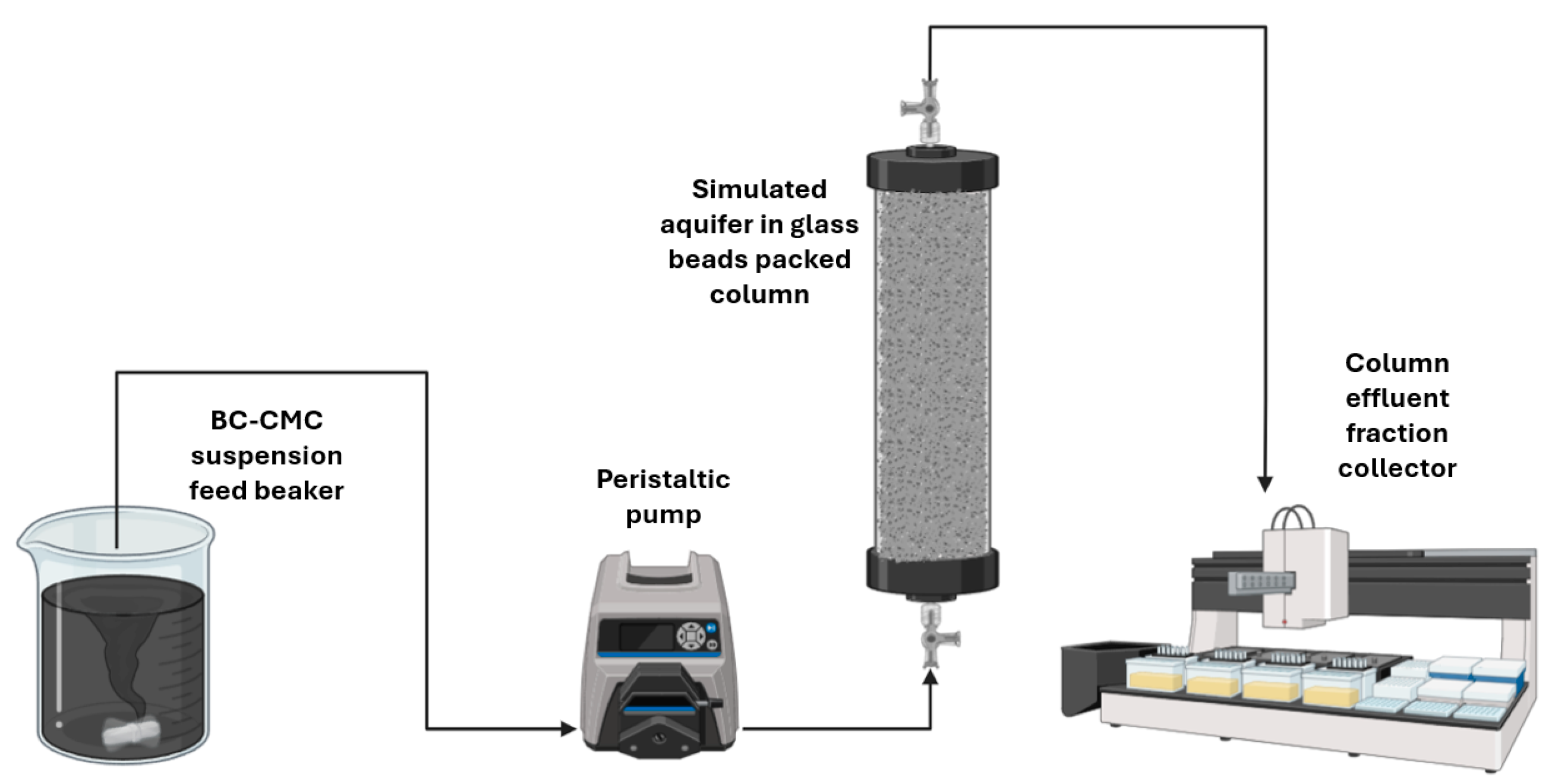
Figure 2.
IPRB process simulation set-up used in this work.
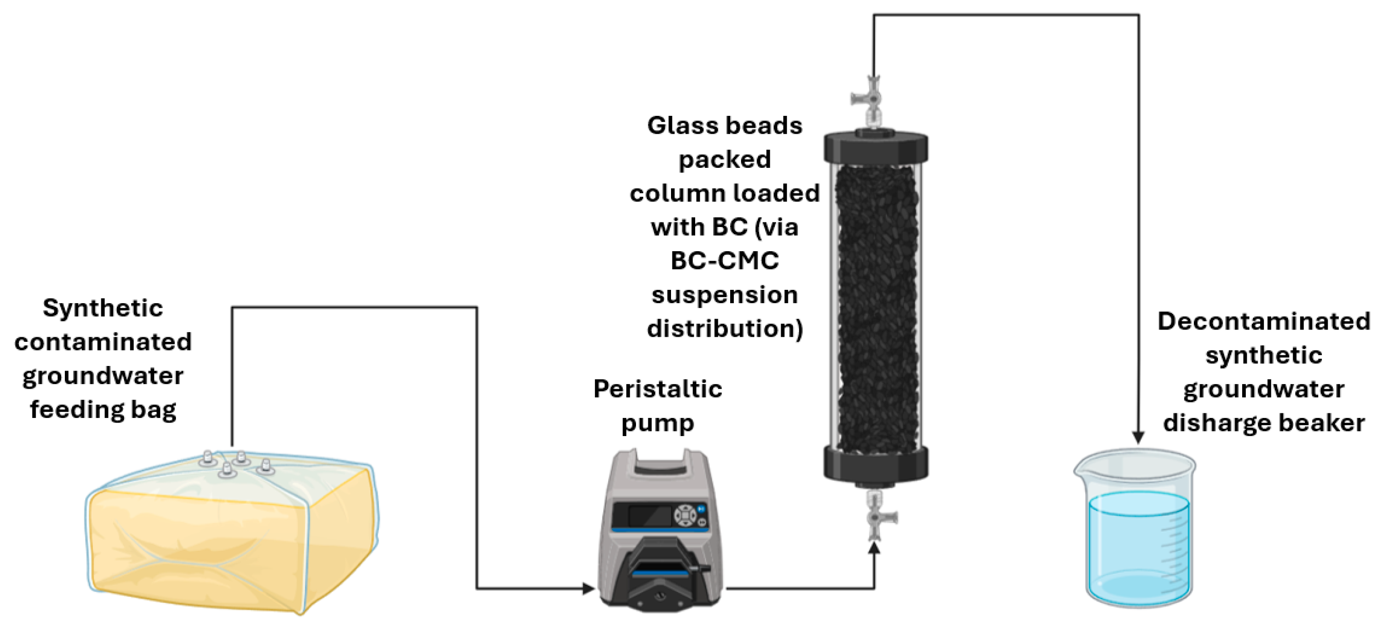
Figure 3.
Stability in aqueous suspension on BC 0.3 g·L⁻¹ @CMC 10 g·L⁻¹ as a function of NaCl concentration over time. Error bars are the standard deviation of three replicates.
Figure 3.
Stability in aqueous suspension on BC 0.3 g·L⁻¹ @CMC 10 g·L⁻¹ as a function of NaCl concentration over time. Error bars are the standard deviation of three replicates.
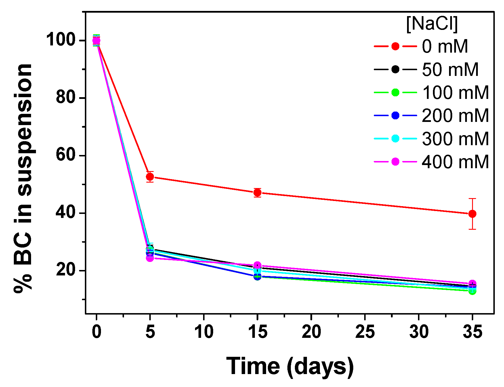
Figure 4.
Stability studies on BC 0.3 g·L⁻¹ @CMC 10 g·L⁻¹ suspension as a function of the pH: (a) UV-Vis stability evaluation. %BC in suspension was calculated as At/At0 at 650 nm; (b) Hydrodynamic size evolution over time.; (c) ζ-potential trend. Error bars are the standard deviation of three replicates. Native pH is highlighted in bold.
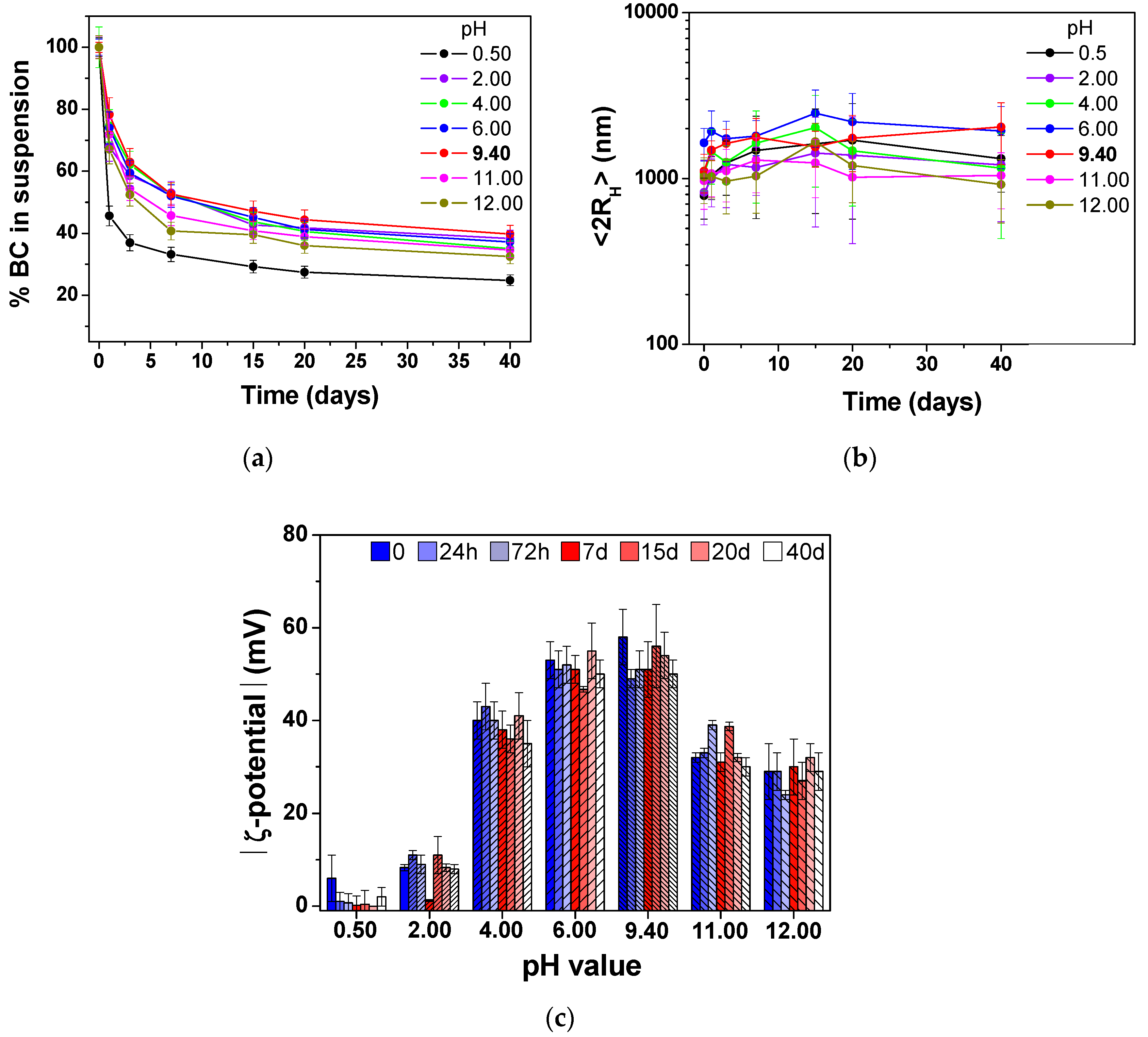
Figure 5.
Plot of the ratio between BC outlet concentration and inlet concentration in the column versus the number of BC@CMC pore volumes fed into the column.
Figure 5.
Plot of the ratio between BC outlet concentration and inlet concentration in the column versus the number of BC@CMC pore volumes fed into the column.
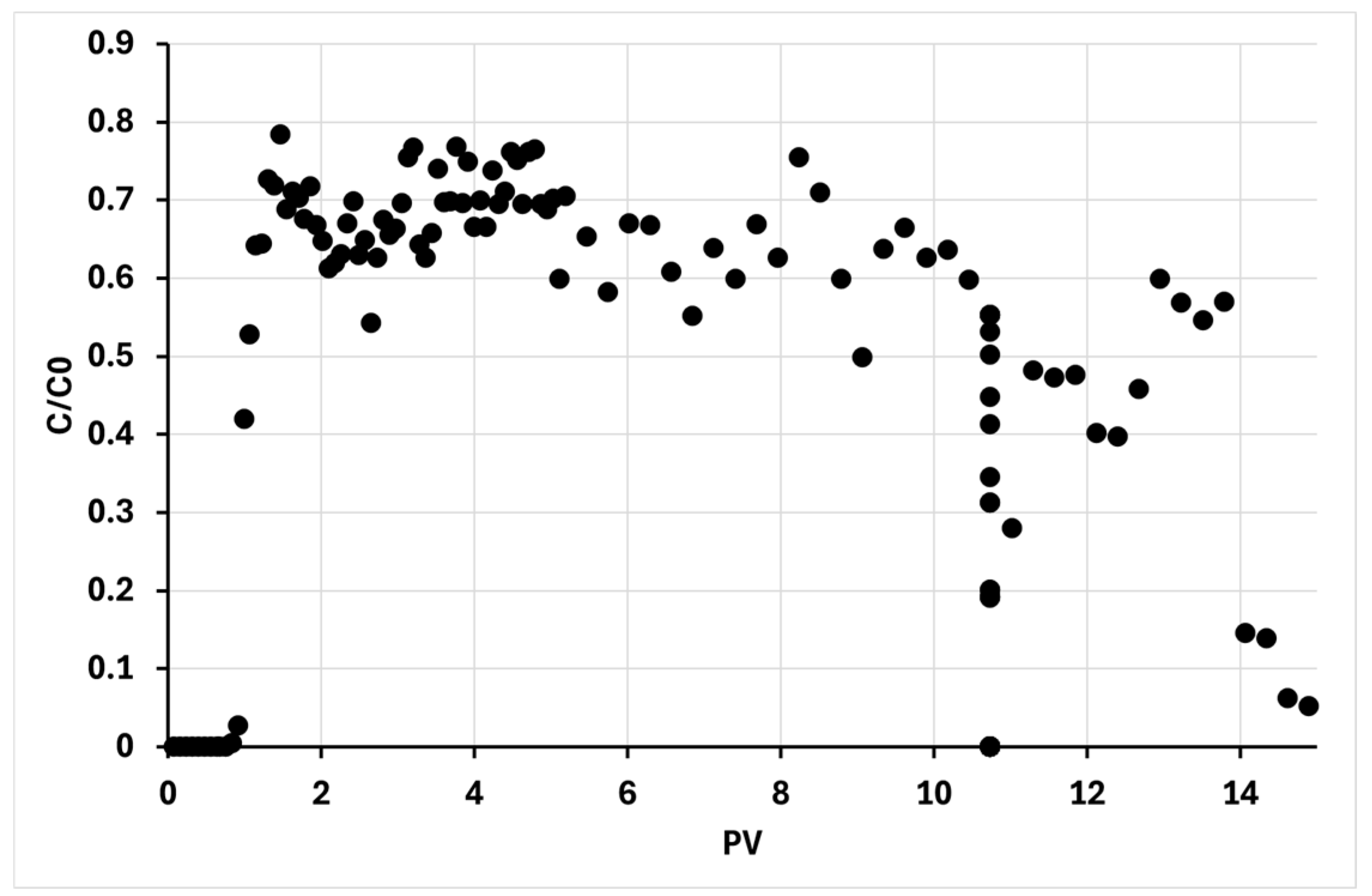
Figure 6.
Visual comparison of the column before and after the BC@CMC breakthrough experiment.
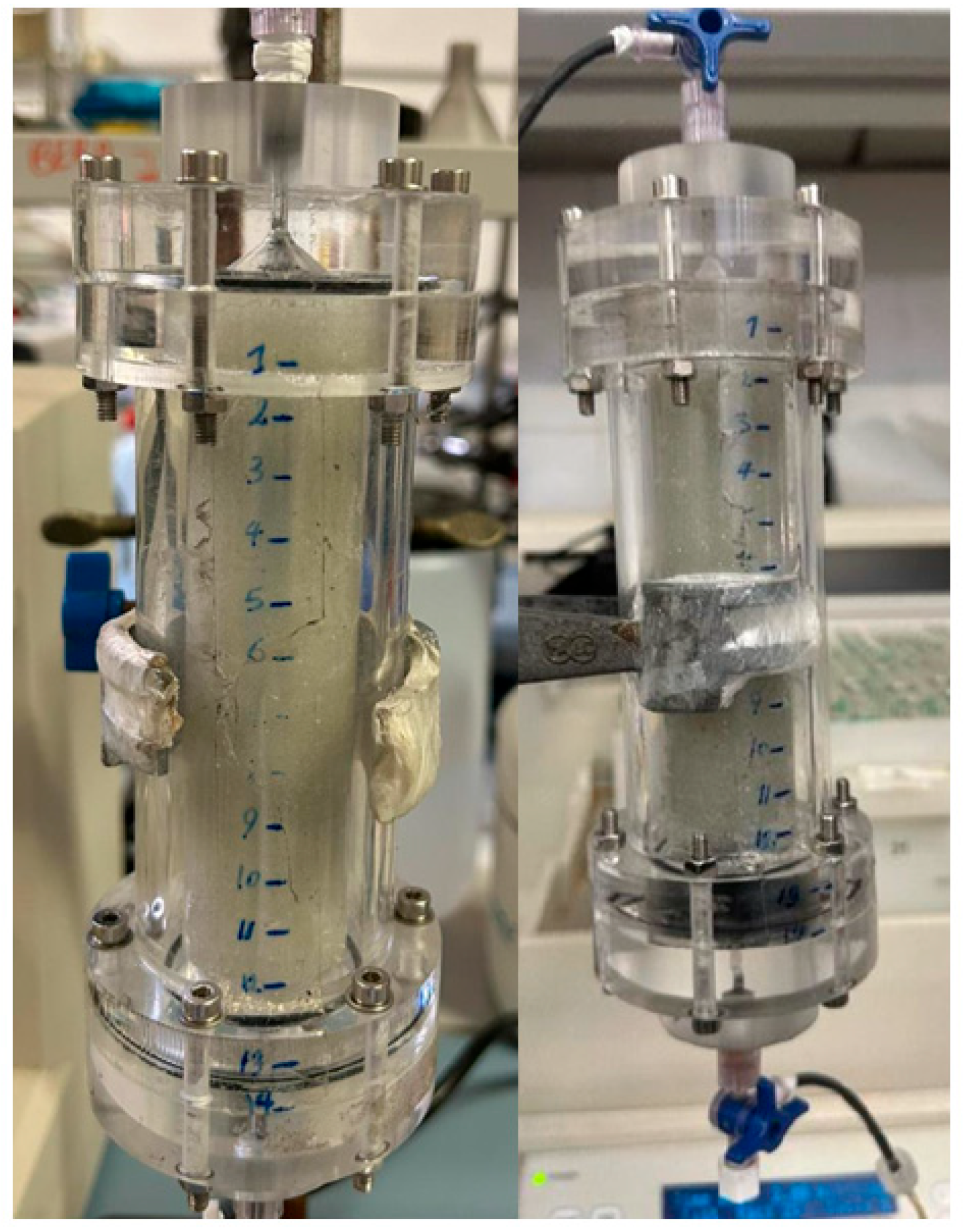
Figure 7.
Filtration of BC@CMC suspension. (a) Picture representing the composite sieved at 50 μm mesh size showing the amount of retained BC; (b) DLS analysis carried out on pristine BC@CMC (magenta line), BC@CMC sieved at 64 μm (blue line), and at 50 μm (red line).
Figure 7.
Filtration of BC@CMC suspension. (a) Picture representing the composite sieved at 50 μm mesh size showing the amount of retained BC; (b) DLS analysis carried out on pristine BC@CMC (magenta line), BC@CMC sieved at 64 μm (blue line), and at 50 μm (red line).
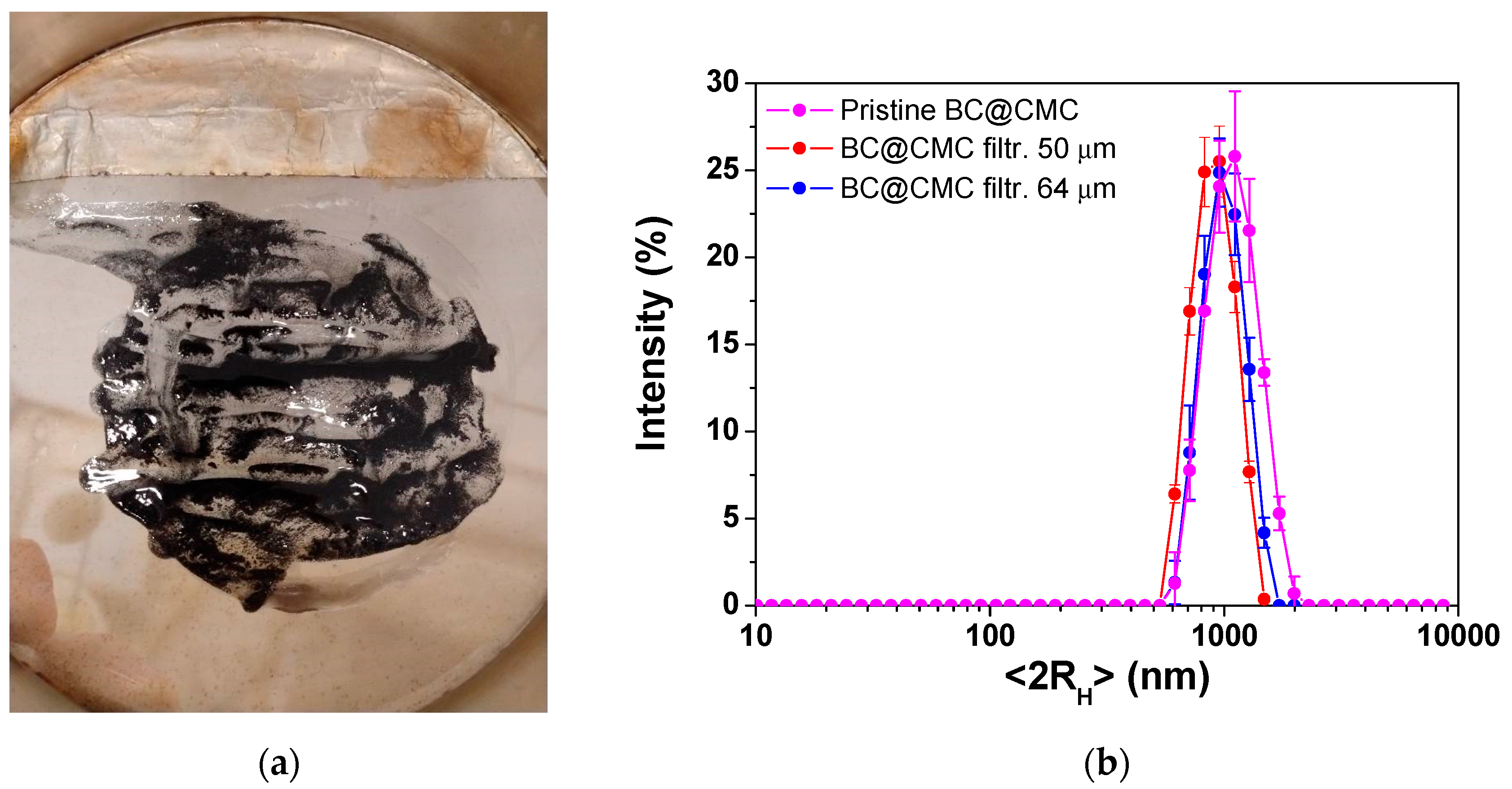
Figure 8.
(a) Plot of the ratio between BC outlet concentration and inlet concentration in the column versus the number of BC-CMC pore volumes fed into the column. The graph shows the trends of three distinct distribution tests coded as follows: F-xx-y-z where xx is the filter mesh size, y is the replicate, and z is the working phase (L for loading and W for washing); (b) Progressive photos of the elution of the first PV of BC@CMC F-64.
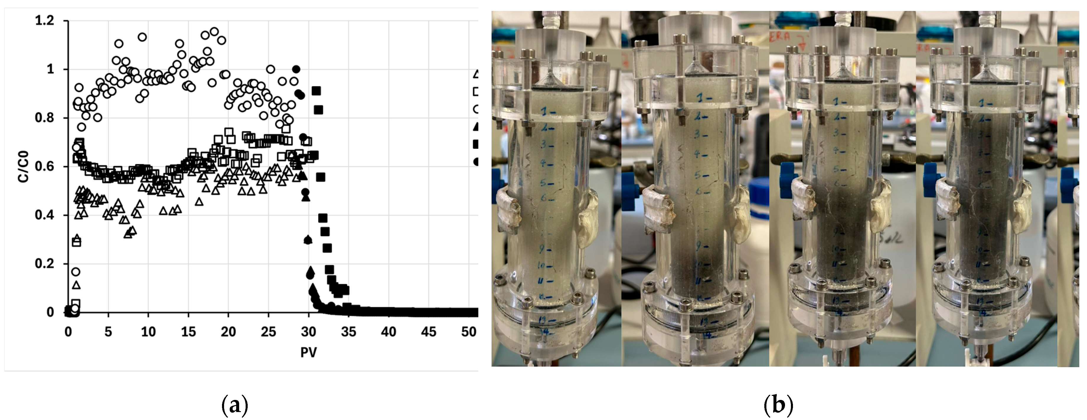
Figure 9.
Plot of the ratio between BC outlet concentration and inlet concentration in the column versus the number of BC@CMC pore volumes fed into the column. The graph shows the trends one distribution test for a BC@CMC 3-10 g∙L-1 filtered on 64 µm mesh sieve during the loading (L) and washing (W) phases.
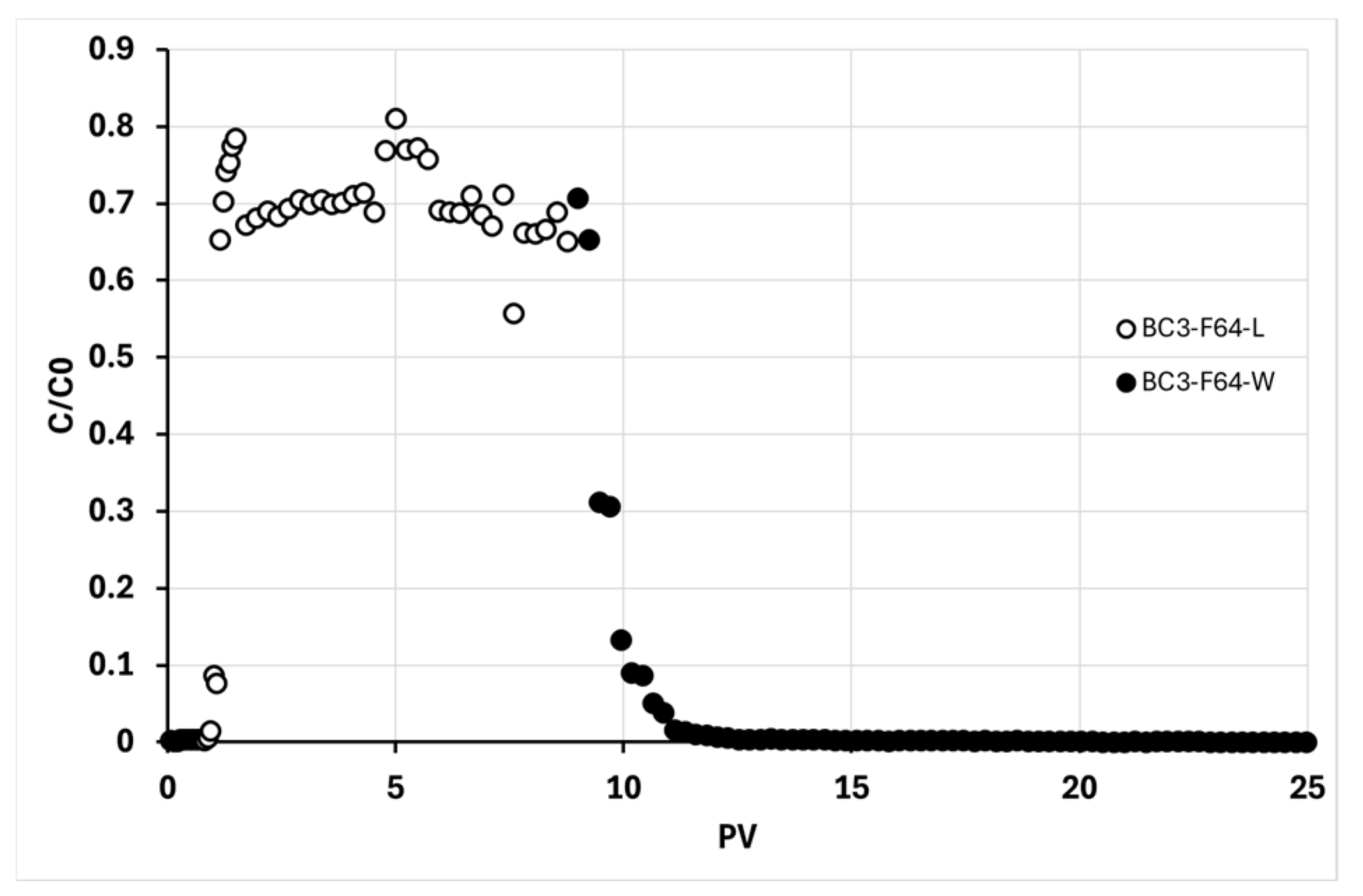
Figure 10.
(a) Test tube used in the BC@CMC F-64 sedimentation tests, specifically a BC1 tube at 96 hours from the start of the test; (b) Average sedimentation values in the superficial layer, grouped based on the observed trends.
Figure 10.
(a) Test tube used in the BC@CMC F-64 sedimentation tests, specifically a BC1 tube at 96 hours from the start of the test; (b) Average sedimentation values in the superficial layer, grouped based on the observed trends.
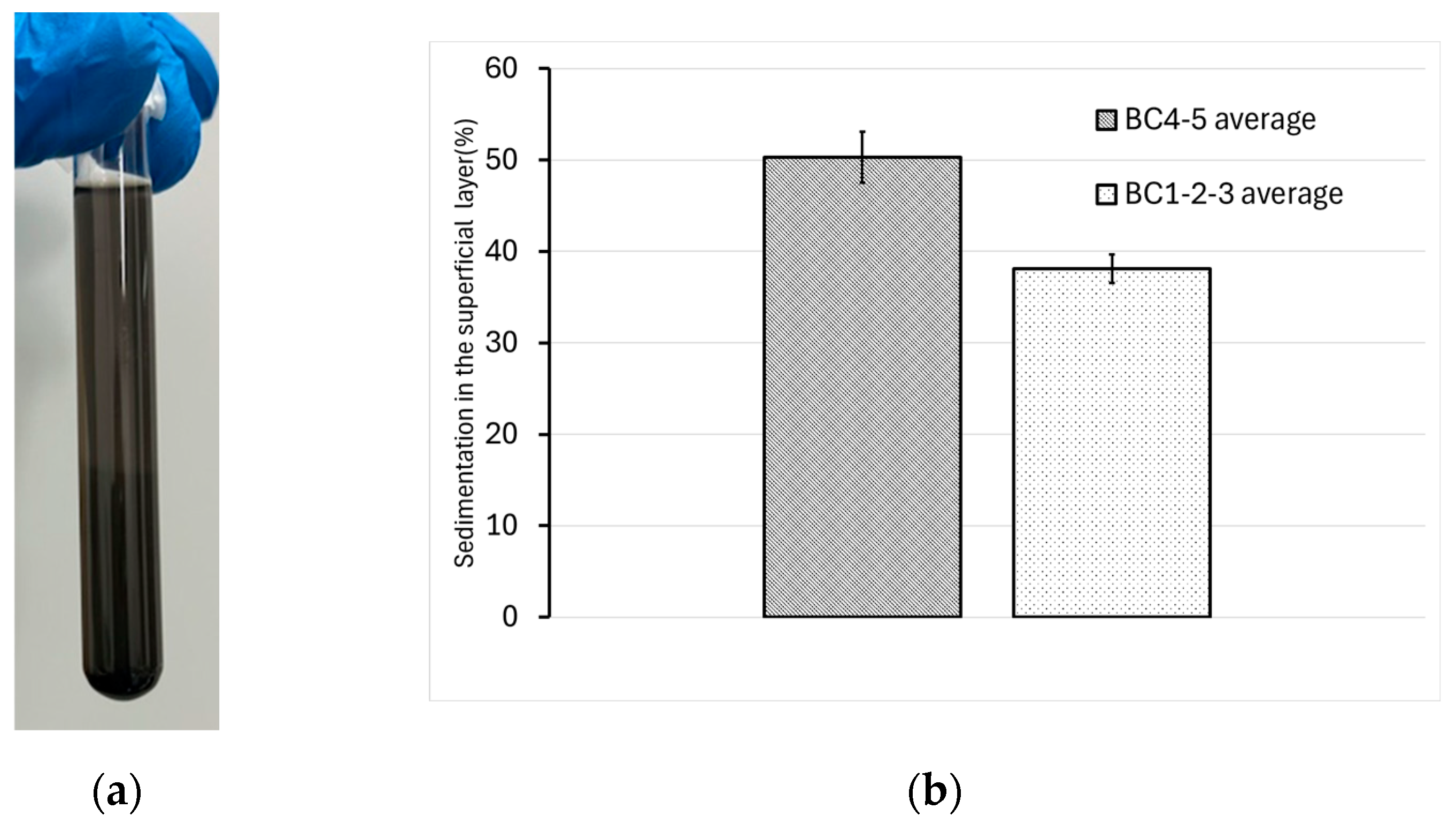
Figure 11.
(a) Comparison of TOL adsorption isotherm trends on BC and AC; (b) Comparison of PCE adsorption isotherm trends on BC and AC.
Figure 11.
(a) Comparison of TOL adsorption isotherm trends on BC and AC; (b) Comparison of PCE adsorption isotherm trends on BC and AC.
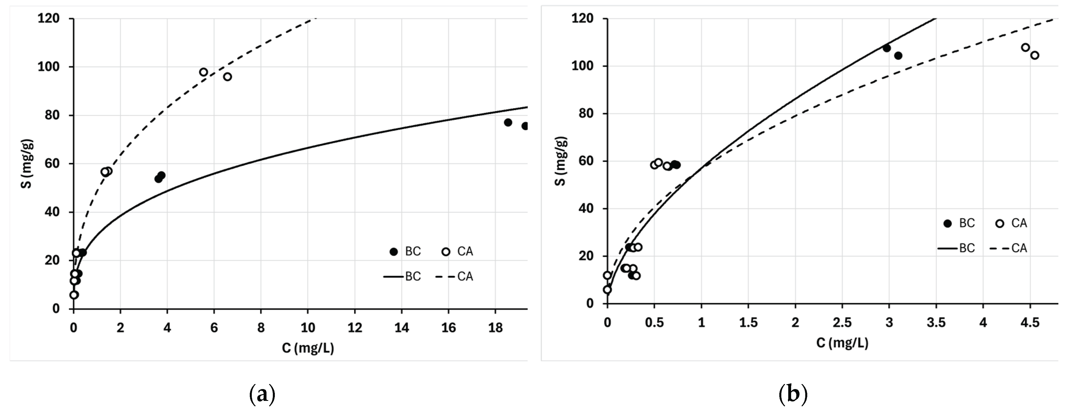
Figure 12.
Comparison between continuous flow of synthetically contaminated groundwater with TOL and PCE through a column loaded with BC via BC@CMC distribution.
Figure 12.
Comparison between continuous flow of synthetically contaminated groundwater with TOL and PCE through a column loaded with BC via BC@CMC distribution.
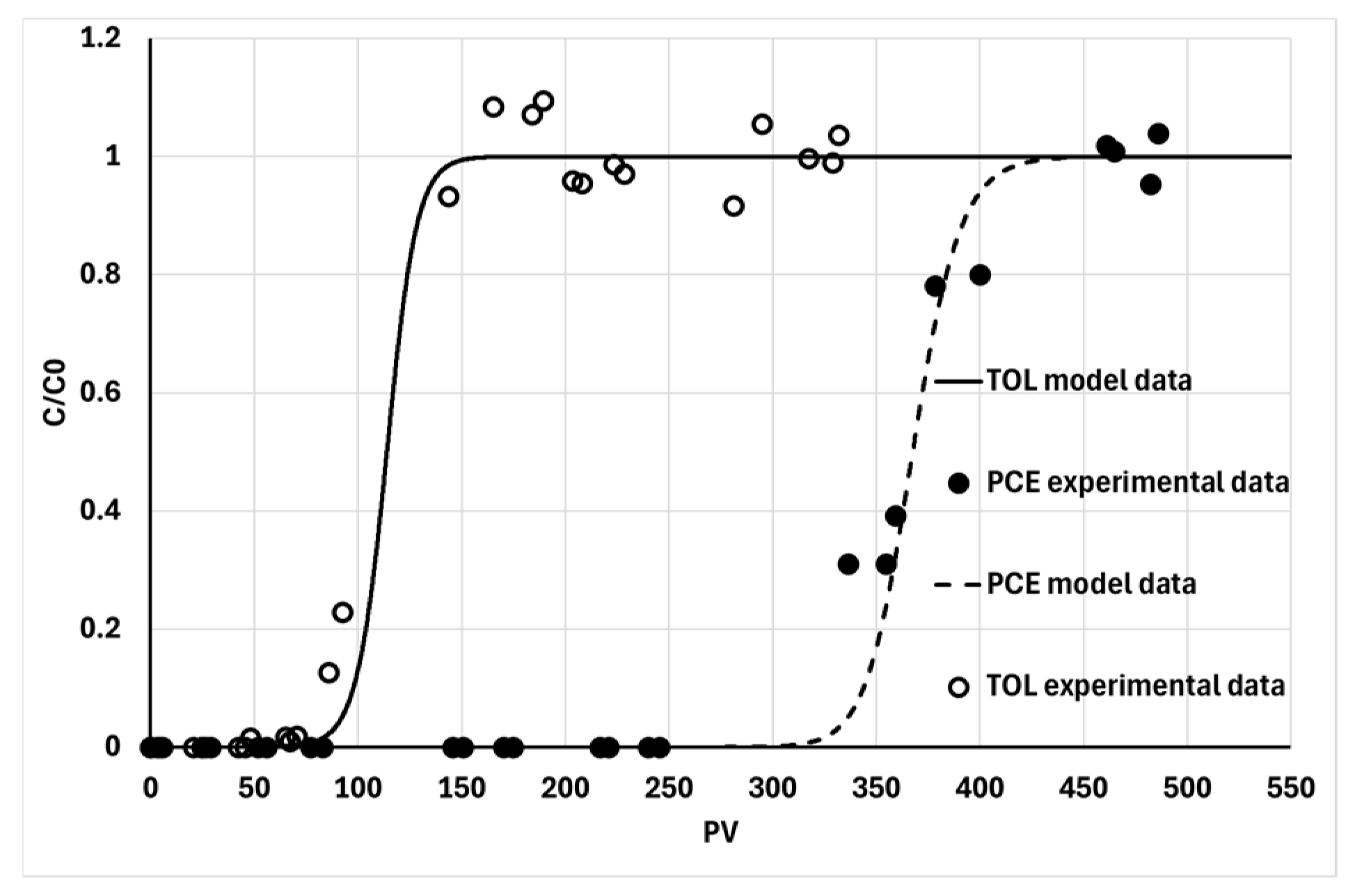

Table 1.
Parameters calculated via mass balance equation (1, 2, 3).
| Parameters → Test runs ↓ |
mBC (mg) | mPV (mg) | fBC (%) |
|---|---|---|---|
| F-50 | 10 ± 7 | 0.30 ± 0.03 | 0.010 ± 0.007 |
| F-64-1 | 300 ± 10 | 9.9 ± 0.7 | 0.29 ± 0.05 |
| F-64-2 | 320 ± 10 | 9.9 ± 0.7 | 0.31 ± 0.05 |
Table 2.
Summary of the final results from the sedimentation tests across the different concentration ranges tested.
Table 2.
Summary of the final results from the sedimentation tests across the different concentration ranges tested.
| Suspension composition | Superficial sedimentation (s) at 96 h |
|---|---|
| BC@CMC 1 – 10 g∙L-1 | 37 ± 4 % |
| BC@CMC 2 – 10 g∙L-1 | 37 ± 1 % |
| BC@CMC 3 – 10 g∙L-1 | 39 ± 1 % |
| BC@CMC 4 – 10 g∙L-1 | 48 ± 5 % |
| BC@CMC 5 – 10 g∙L-1 | 52 ± 3 % |
Table 3.
Summary of the Freundlich fitting curve parameters for the BC isotherms.
| Adsorbents → | BC | AC | ||
|---|---|---|---|---|
|
Parameters → Test runs ↓ |
KF (Ln·gADS-1·mgCONT1-n) |
n (adim.) |
KF (Ln·gADS-1·mgCONT1-n) |
n (adim.) |
| TOL | 30 ± 2 | 0.34 ± 0.02 | 49 ± 2 | 0.38 ± 0.02 |
| PCE | 57 ± 4 | 0.59 ± 0.05 | 57 ± 5 | 0.48 ± 0.05 |
Disclaimer/Publisher’s Note: The statements, opinions and data contained in all publications are solely those of the individual author(s) and contributor(s) and not of MDPI and/or the editor(s). MDPI and/or the editor(s) disclaim responsibility for any injury to people or property resulting from any ideas, methods, instructions or products referred to in the content. |
© 2025 by the authors. Licensee MDPI, Basel, Switzerland. This article is an open access article distributed under the terms and conditions of the Creative Commons Attribution (CC BY) license (http://creativecommons.org/licenses/by/4.0/).
Copyright: This open access article is published under a Creative Commons CC BY 4.0 license, which permit the free download, distribution, and reuse, provided that the author and preprint are cited in any reuse.


