Submitted:
24 October 2025
Posted:
29 October 2025
You are already at the latest version
Abstract
Cosmic rays are fully ionized nuclei, electrons plus rare particles having extreme high energies with a characteristic energy spectrum up to 3 x 10²⁰ eV. They move and reside in the Galaxy with a lifetime of 15 million years transporting a positive electric charge of about 1031-1032 C. The immense grid of positive electric charges of about 1050 particles necessarily generates an electrostatic field in the entire Galaxy. This work present five diverse models to quantitatively describe the Galactic electrostatic field and the related potential. Analytical formulae and tabulated values from computer calculation of the Galactic electric field are explicitly reported for the first time. Any of the five models have field intensities close to one V/m and electrostatic potentials in the range 1019-1020 V. The anchorage of the calculation to the observational data is delineated in the last Section.
Keywords:
galactic electrostatic field
; electrostatic potential in the galaxy
; cosmic rays and galactic electric field
; acceleration of cosmic rays
; dark matter
1. Introduction
The main reasons to admit a permanent electric field in the Milky Way Galaxy have been reported at the 37 held in Berlin in 2021, Germany [1]. These reasons, arranged in a logical inference and based on experimental data, take advantage of the energy density of cosmic rays, about 1 /, and the applied to a system of charged particles. Cosmic nuclei are fully ionized atomic nuclei and globally form a huge system of charged particles extended up to the Galaxy radius of m, 15 , and elevations above the Galactic midplane of 2 . Electrons are only 1.5 per cent of the cosmic-ray population at about 10 and still less electron fractions are observed at higher energies up to 1 [2,3] and above. Recently (2024), in Namibia, the HESS gamma-ray telescope observed an electron fraction of about 0.02 per cent of the proton flux at 40 .
This work, in order to redundantly prove the existence of the , contrary to the previous one [1], makes the opposite move: electric fields of simple charge configurations are reliably computed from and, then, patiently connected to pertinent features of cosmic rays measured by many experiments.
The two essential pertinent features are: ( ) the position of cosmic-ray sources in spiral galaxies. The is a spiral galaxy. Its radio emission and that from nearby spiral galaxies as well, particularly synchrotron emission, unambiguously determine the position of the sources (see, for example, ref. [4,5,6]). Sources are located in molecular and atomic clouds and store the negative charge (the subscript w is for widow electrons). Orbital electrons lost by the accelerated cosmic-ray nuclei leaving the sources retain the negative charge and are referred to as . Cosmic-ray nuclei are fully stripped nuclei and transport the charge (the subscript cr is for cosmic rays) being, = -.
() Cosmic nuclei do have overwhelming kinetic energies in comparison to any sort of cosmic materials. These high energies enable cosmic-ray nuclei to propagate far away from the sources where they are generated. As a consequence, the motion of the nuclei creates a halo of positive electric charge around the negatively charged sources because cosmic-ray nuclei transport and disseminate only positive charge. In essence: halo size is larger than source size both structures storing the same opposite charge, = - and this spatial mismatch, ultimately, generates the Galactic electric field.
All cosmic-ray nuclei circulating in the transport the total positive charge in the range - C evaluated elsewhere [1]. In order to easily intercompare the results of different calculations, the nominal charge = - = C 1 is arbitrarily adopted lying in the range - [1] and nominally and shortly set at C. The total number of cosmic rays, , circulating at a given instant in the is about ≃ /q = /()×(1.21) = where q is the average electric charge per cosmic-ray nucleus and = from cosmic-ray data. Here is an order of magnitude estimate.
A highly schematic picture of the positions of the negative and positive charges in the arbitrary spherical volume of galactic size is in Figure 1. This picture reflects the facts and in the sense that the negative charge occupies the central region while the positive charge lies peripherally.
Five diverse charge configurations (Figure 2) are examined in this study, all with total zero charge, namely, = -. The simplest charge configuration is the double, concentric spheres with constant charge density shown in Figure 2-a (Section 2). The second configuration (Section 3) consists of two concentric spheres: a uniformly negatively charged sphere surrounded by positively charged spherical halo with decreasing density from the center (Figure 2-b).
The third configuration (Section 4) derives from the second one: the internal sphere storing the negative charge is replaced by a flat disk of volume 2 h where h is the half thickness of the disk and its radius (Figure 2-c).
The fourth configuration (Figure 2-d and Section 5) has no spherical form : it consists of two highly squashed, concentric cylinders with the same radius and different heights, h and (h for halo of positive charge). The fifth configuration (Figure 2-e and Section 6) consists of six discrete negative pointlike charges constrained by the charge equality = - = C and a size of about 15 . The number of six charges is thoroughly arbitrary but uncritical. A positively charged halo with decreasing charge density from the center (Figure 2-e) completes the structure.
2. The Electric Field Of Two Concentric Uniformly Charged Spheres
Imagine a sphere of radius with negative electric charge uniformly distributed over its volume. The intensity of the electric field (r) is straightforwardly determined from elementary :
where = F/m and = / (4/3) is the negative charge density in the sphere. Equation (1-a) applies in the range r≤ while (1-b) in r≥. Here, of course, it is = = - C.
Due to the spherical symmetry, the field intensity (r) is zero at the center, then, it augments with increasing radial distance r according to (1-a) up to the sphere radius as displayed in Figure 3-a. At radial distance r ≥ the field strength decreases as 1/ as it is well known.
Consider further a second sphere of radius of positive electric charge and density = / (4/3) concentric to the sphere of radius . The corresponding electric field (r) has expressions analogous to those (1-a) and (1-b) except for the positive charge sign, and .
The total field E(r) is the sum of two components: E(r)= r) + r) at any distance r from the sphere center. If = - and = the field strength is, of course, null everywhere. Whenever a slight offset in the positive and negative charge distributions occurs, a finite electric field sets on inside the sphere.
For example, the arbitrary parameters, = 5 , = 3 = 15 , = - = C yield charge densities = - C/, = C/ and field intensities (15 ) = 1.0819 V/m and (5 ) = - V/m, respectively. The radial profile of the total electric field, E(r), is shown in Figure 3-a (blue curve) along with (r) (red curve) and (r) (green curve). The field vanishes beyond = 3 = 15 as shown in same figure.
The potential for the negative charge reads:
Equation (2-a) applies in the interval r ≤ while (2-b) in r≥. Analogous equations hold for the positive charge .
This is the simplest conceivable charge configuration with a vague kinship to cosmic-ray data. The vague kinship are facts and (Section 1), namely, the negative charge predominates in the core of the spherical volume while the positive charge in the periphery.
3. Two Concentric Spheres With Unequal Profiles Of Charge Densities
A step forward from the previous charge configuration toward physical reality is the removal of the uniform charge distribution of the positive charged halo of the cosmic-ray nuclei.
The displacement of cosmic-ray nuclei from the sources of finite size produces a charge density2 featured by 1/r where r is the distance from the source up to a characteristic distance R. The simple behavior 1/r is in the radial interval r< R. Accordingly, the positive electric charge density per unitary volume, (r), reads:
where k is a constant. From elementary the electric field intensity (r) generated by the charge distribution (3) is constant, directed outwardly and it is:
where is the total positive electric charge transported by cosmic rays and the characteristic distance of the propagation. For example, with = C and R = 300 , at any arbitrary radial distance satisfying, , it turns out: = V/m.
As cosmic-ray sources of this 2 retain a total negative electric charge, = having spherical symmetry of diameter 2, in a generic point r such that , the intensity of the resulting electric field E(r) is:
where / is the field strength of the negative charge only, designated by (r). Because of the postulated spherical symmetries of the positive and negative charge distributions and the common origin , the electric field (r) vanishes beyond the distance R.
Inside the sphere, 0 ≤r≤, the field intensity is: / 4 similarly to Equation (1). Accordingly:
which coincides with the outer field given by Equation (5) at the point r = = 15 . Hence, the electric field intensity E(r) for r<R is always less than (r) by the constant amount = / 4. The profile of E(r) versus radius is shown in Figure 4. For example at the distance r = = 15 it turns out, () = V/m, which is about 400 times greater than (r) of Equation (6) with R = 300 . For any other distances r< the ratio (r)/ (r) decreases.
In the region, 0 ≤r≤ = 15 of the spherical volume (4/3) = , the mean energy of the electrostatic field given by equation (5) is and, accordingly the mean electrostatic energy density is /.
The radial profile of the electrostatic potential related to the electric field represented by Equation (5) and (6) , in the same conditions specified above, setting D≡/4 = V takes the form:
Equation (7-a) holds for while the (7-b) for . Figure 5 shows the profile of the potential (black curve) in the range, for = 15 and n = 20 being n = R/. The classical normalization condition of zero electrostatic potential at very large distances has been adopted.
4. A Positively Charged Sphere Concentric To A Negatively Charged Disk
Sources of cosmic rays in the Milky Way Galaxy like other nearby spiral galaxies are distributed on a thin disk. This fact is proved by redundant evidence via radio, infrared and optical emission from regions, molecular clouds and neutral Hydrogen clouds as recapitulated in Section 1 by the fact . As a consequence, a thin disk, instead of a sphere, better adheres to the spatial dissemination of the cosmic-ray sources.
An artistic view of this charge configuration ( 3) is delineated in Figure 2-c.
The negative charge has a cylindrical symmetry and, therefore, the electric field and potential have two components: radial r and elevation z (Figure 2-c).
Consider a disk of center , radius and thickness 2h with = 15000 and h=125 . Let the negative charge = - C be uniformly distributed inside the disk volume, and assume further, that the positive charge of the cosmic rays (positively charged nuclei) diminishes in the whole space as k/r following equation (3) up to the maximum distance from the center R. Here r is the generic distance from the center and k a suitable constant. The calculation adopts, R = 300 , k = - /2 = -C/ and a total positive charge equal to that of widow electrons, . This geometrical form with the negative electric charge enshrouded by the charged cocoon of cosmic nuclei would imitate the electrostatic structure of a common disk galaxy like the Milky Way Galaxy or better than the concentric double sphere with zero charge previously examined ( 2 in Section 3).
The function k/r is equal to that of the crude surrogate of the spherical galaxy expressed by Equation (3) and it produces a constant electric field intensity of V/m if = C and R = 300 , always directed outwardly, as previously remarked.
The electric field of this structure denoted by can be decomposed in a radial and vertical (also elevation z) components, and , respectively, in such a way that: = + . The intensity versus radius r up to 25 is shown in Figure 6-a. As it is quickly realized, in the range 0 <r< the field profile turns out to be concave relative to a linear trend (for instance the trends represented in Figure 3-a and 4 in the radial range 0 <r< 15 ). Thus, the field strength vanishes at the origin and takes the maximum value of - 3.7 V/m on the rim e. g. r = = 15 .
The intensity versus elevation z at the four arbitrary radii r = 0, r= , r = and r = are shown in Figure 6-b. The profile for r = 0 (green curve) joins the profile in Figure 6-a (green curve) in the range <r< 250 and completes it. For r = 0 the field strength attains its maximum of 3.38 V/m at elevations z above 125 . As expected for an ideal, infinite uniformly charged slab, the field strength is almost constant close to the slab (highly flat cylinder in the present case) even with a finite slab.
Assimilating the Milky Way Galaxy to this structure ( 3), in the nominal position of the solar system, i. e. r = and z = 0 it is: = V/m. The electric field inside the disk, around the solar system (r = and z = 0) in the plane xz normal to the Galactic midplane xy is visualized by the vector array in Figure 7. Note that the unit length in the x and z axes differ by a factor 80.
The electric field of 3 has an approximate spherical symmetry in regions far away from the center and imitates the spherical symmetry of the double sphere with zero charge ( 2 in Section 3). For example, in the position z = 400 and r = 0 it results, = V/m while for r = 400 and z = 0 it results: = V/m so that: - = V/m. Given the smallness of this difference it turns out that at large distance from the center the field strength is almost independent from the direction.
5. Two Concentric Squashed Cylinders With Positive And Negative Charge
In 4 the electrostatic field (r,z) results from the sum of the fields of two separate single disks which are denoted by (r,z) for the charge and (r,z) for the charge being = + . For sake of simplicity,
two uniform charge distributions in the two volumes 2h (disk) and 2 (halo) are used in the calculation having, respectively, charge densities = C/ and = C/.
To begin with, the field strength E(r,0) along the radial direction for z = 0, and E(0,z) along the z axis for r = 0 are calculated. The x axis is chosen as generic radial direction. This choice does not lack of generality as the field (r,z) has cylindrical symmetry. These two field profiles, to be evaluated along two particular directions, facilitate the description of (r,z) at any space point inside and outside the .
Radial field profiles, E(r,0) versus r, are shown in Figure 8 (blue curves) for = 1, 2 and 3 . For example, for = 2 the field intensity is almost constant in the range 3 ≤r≤ 9 , then rapidly increases, reaching the maximum of 0.55 V/m at the radial distance r==15 , then, as expected, attenuates as any electrostatic body with of finite roundish form.
The field profiles in elevation, E(0,z)/4 versus z, are shown in Figure 8 (green curves) for = 1, 2 and 3 . Field strengths are reduced by a round factor 4 to facilitate the visual comparison with radial strength E(r,0) in the same figure. The field (0,z) has maximum intensity for z≤ 1 and direction toward the disk interior. For instance, at = 1 the maximum of E(0,z) is /m at the elevation z= ± 175 . Beyond the distance of 1 the direction of the field (0,z) points toward the exterior. Field intensity spans the interval 1-5 /m, lower by 3 orders of magnitude than that in the range r≤ 1 which however is not visible in Figure 8.
Let us examine some aspects of the individual fields and quite useful in the following. Generally, for a preassigned radial distance and a halo size , the field intensity (0,z) decreases if z ≤ . For instance, for z = 1 and = 3 , the field intensity (0,3) is /m while for z = 1 and = 5 the field intensity (0,5) is /m.
Whenever is greater than h, the intensity (0,z) in the range z≤ is lower than ∣ (0,z) ∣ in the same range and the resulting field = + is directed toward the disc midplane. On the contrary, for z≥ the inequality, (0,z) ≥ ∣ (0,z) ∣ holds and the direction of the field is points outwardly. In the specified conditions E(0,z) vanish and changes sign. Consequently, there exists a coordinate ±z labelled for which the field (0,z) vanishes and changes sign. Of course, is a function of r.
The numerical example just discussed is very general indeed and the field inversion takes place in the whole range 0 <r≤ 15 and not only at r = 0. The behavior versus r for = 1,2,3 and 4 is shown in Figure 26 of ref. 8.
If the field configuration is examined not only for r = 0 but for an arbitrary value of r in the intervals, 0 <r≤ 15 and z≤ it results that the field is directed toward the center (exactly toward the Galactic midplane) and for z≥ the field is directed toward the exterior.
Notice that the values of the electrostatic potential V(r,z) for the two squashed, concentric, coaxial cylinders (Figure 9 and Figure 10 of 4) are thoroughly different from those of the Models 1 and 2 (Figure 3-b and Figure 5). As an example, the potential difference onto the Galactic midplane between the disc rim = 15 and the solar system at =, namely, [V(,0) - V(,0)] is V for 1, V for Model 2 with R = 300 , = 15 and n = R/ = 20, V with R = 60 , = 15 , n = 4 and, finally, V for 4 with = 1 and V for 4 with = 2 . Such differences are intuitively and qualitatively expected from the charge distribution sizes.
Improvements of 4 based on observational Astronomy are suggested in the legend of Figure 11.
6. Discrete Charge Array Of Galactic Dimension
The electrostatic structures of 1 and 2 have a perfect radial symmetry. This implies that the electric field is strictly zero beyond the radius R, namely, beyond the maximum extension of the halo of positive electric charge transported by cosmic nuclei. What happens instead, if the radial symmetry is altered, yet maintaining the condition = - ?
A multipolar electric field extending in all the space is generated. Here it is desired to familiarize with this assertion with a numerical example by the examination
of a very simple electrostatic structure devoid of planar and spherical symmetries. A system of six pointlike negative charges is shown in Figure 12-a. The total amount of negative charge is = - C. The six spheres lie in the xy plane with origin as shown in the same figure. Each sphere stores the charge /6 and it is placed at the following (x, y, z) coordinates: (-,0, 0); (,0, 0); (a,0, 0); (,0, 0), (0,, 0) and (0,a, 0) being a the characteristic size of the system. Setting a = the maximum extension of the structure is 2 a = 15 . The spherical halo of positive charge with density (r) given by the Equation (5) with R = 300 overlaps the negative charge. The total charge within R is zero i. e. = -. To simplify Figure 12-a the positive charged halo is not shown but it is sketched in Figure 2-c.
Beyond 2a and within R that is, between 15 and 300 the electric field strength behaves similarly to that of Figure 3 of the double concentric sphere with zero charge. There are however slight differences due to the absence of the radial symmetry of the system shown in Figure 12-a. The electric field on the xy plane at the two radial distances 200 and 300 is shown in Figure 12-b by a vector array.
The direction of the electric field along the x axis points always to the center while along the y axis, at the characteristic distance R - i (i for inversion and i> 0) the field changes direction. In the specified conditions it turns out, i = . Beyond the distance R - i = 94 along the y axis, the electric field points always outwardly. The electric field can be decomposed in a radial and normal component. In xy plane at the approximate distance R (Figure 12-b) there is a line defined by all the points for which the radial electric field vanishes. This line intercepts the coordinate y = - i = 94 and x = 0 and mimics a geographical divide: cosmic nuclei born and emitted beyond the line are accelerated toward the exterior. This region and the symmetric one are colored by yellow in Figure 12-b and filled with red arrows.
On the contrary a cosmic nucleus, initially at rest and located at any arbitrary point along the x axis, will encounter an electric field always in the same favorable direction, precipitating toward the center of the electrostatic structure. This occurs not only along the x axis but in the entire annular region around the x axis beyond R = 300 .
The electrostatic potential generated by the 6 negative charges in a generic point along the x axis at the distance d from the center is:
Here it is desired to compare the electrostatic potential of the point (d, 0, 0) with that in the point (0, d, 0) of coordinate d in the vicinity of R= 300 as Figure 12-a (not in scale) shows. Setting arbitrarily d = 300 then, it turns out: = - V. The potential generated by the positive charge is given by the Equation (7-a), = V and, hence, the resulting potential in is: = - = -V. Thus, if this enormous electrostatic potential were converted into kinetic energy of a cosmic proton traveling between and the acquired energy is . This elementary example highlights the huge energy gains and losses of cosmic nuclei roaming Galactic and intergalactic regions.
As the ideal and smooth charge distributions of Models 1,2,3 and 4 do not perfectly materialize in real galaxies, some features of the discrete charge distribution of 5 highlight the prominent common features of the other four models. For instance, galactic electric fields extend to all the space and do not vanish beyond the typical sizes of the charge distributions as it occurs in 1 and 2 ( i.e., beyond 30 and 300 , respectively).
Notice, finally, that both the electric field intensity and related electrostatic potential of the 5, inside and outside its characteristic size 2a = 15 , are comparable to those of the four models 1, 2, 3 and 4.
7. The Permanent Regeneration Of The Galactic Electric Field
In order to dissolve or nullify the electric field, , either the electric charge of the cosmic rays and that at the sources have to disappear from the or the electric generator powering cosmic-ray circulation has to cease operation.
The disappearance of could occur only by charge neutralization accomplished by a hypothetical particle population transporting negative electric charges = - = - C. This hypothetical population of negative charged particles has to exactly and finely compensate the positive charge = C over the entire volume. The compensation mechanism has to accomplish charge neutralization at any sites of the , not only globally. In fact, any disjoint charge distributions would generate a global electric field as it simply and unquestionably emerges from the two concentric charged spheres having an arbitrary offset in the charge distributions (Figure 2-a and Section 2).
The only negative charged particles with infinite lifetimes are electrons and antiprotons out of more than 300 elementary charged particles presently known. Electrons due to synchrotron emission in the magnetic field neither spatially nor energetically could accomplish such a chimeric compensation. The flux of cosmic-ray antiprotons are 4 orders of magnitude lower than those of cosmic-ray nuclei and, therefore, do not dissolve whatsoever the electric field.
Without an appropriate refurbishment of fresh cosmic rays, the electric field would disappear in a cosmic-ray lifetime of (10-20) years . The observed stability of the cosmic-ray intensity dictates that the field is continuously regenerated by new born cosmic rays. The existence of cosmic rays and the stability of their intensity in the last billion years is a fact (see, for example, potassium data [10]) which necessarily implies the existence and stability of the electrostatic field.
The energy source powering cosmic-ray circulation ultimately derives from stars via photon ionization of interstellar gaseous materials. This theme is outside the perimeter of this work and is dealt with in [8] (see 10 for the energy sources and 12 for an electric circuit imitating the cosmic-ray circulation through the ).
The arguments above lead to the plain conclusion that the electric field not only exists but it is an inviolable structure of the .
8. Compendium, Context And Conclusion
electric fields and related potentials have been computed with a size of m (15 ) and the total electric charge transported by cosmic rays which is in the range -C [1], nominally set in this and other studies at C (see footnote 1). These two input data have a solid, irrefutable empirical basis [1,8]. The computed intensities of the electric field span from fractions of V/m up to a few V/m and they are shown in Figure 3-a, Figure 4, Figure 6 and Figure 8. These field intensities through the size of m generate electrostatic potentials in the interval -V shown in Figure 3-b, Figure 5, Figure 9 and Figure 10.
As far as the existence of the electric field is at stake, all the geometrical forms of the five models presented in this paper produce similar results. Only when fine features of the electric field have to be discerned, different models become relevant. For example, if the spectral index
of 2.65 of the cosmic-ray energy spectrum has to be predicted and correctly calculated, model 4 (two highly squashed concentric cylinders) offers the best agreement with cosmic-ray data (see [8] 9 and 13).
Notice that quiescent, unbound protons with charge q prone to the electrostatic potential, V(r), convert in cosmic-ray protons of maximum energies, qV = q [V() - V() ] where V() and V() are the potentials at the radial distances and , respectively. Adopting the electrostatic potentials evaluated in this work and the Galactic disk radius of 15 , it turns out: qV≃-, order of magnitude. From this, it descends a precious signature in the cosmic-ray energy spectrum: above the energy qV no cosmic-ray proton is expected to circulate in the because qV is the maximum energy achievable by protons. For instance, if = (solar circle radius) and = 15 (disk rim) then, in the 4, V = V() - V() = - V + V = V for a halo hight = 2 and V = V for a halo hight = 1 . These maximum energies entail a recognizable break or suppression in the smooth cosmic-ray energy spectrum above the ankle energy of as displayed in Figure 13.
It is a notable fact that these maximum cosmic-ray energies have been observed with the precise and unsurpassed energy resolution of the Auger experiment [12] in the range 7-16 per cent in the energy band -. The break reported by the Auger experiment is at [11] as attested by Figure 13. Only the unsurpassed energy resolution of the Auger experiment made possible the identification of the break in terms of the electrostatic potential and, concomitantly, to dismiss the GZK [13,14] interpretation of the same break. The HiRes Collaboration observed the or at the energy of [15] and interpreted it as effect. This interpretation was reiterated by the Telescope Array (hereafter TA) experiment [16]. The critical theme of energy scales of the and instruments has been discussed elsewhere [17]. The nature of the spectral break at has been elucidated in 2013 [18], in 2017 [19,20] and precognized in 2009 [21].
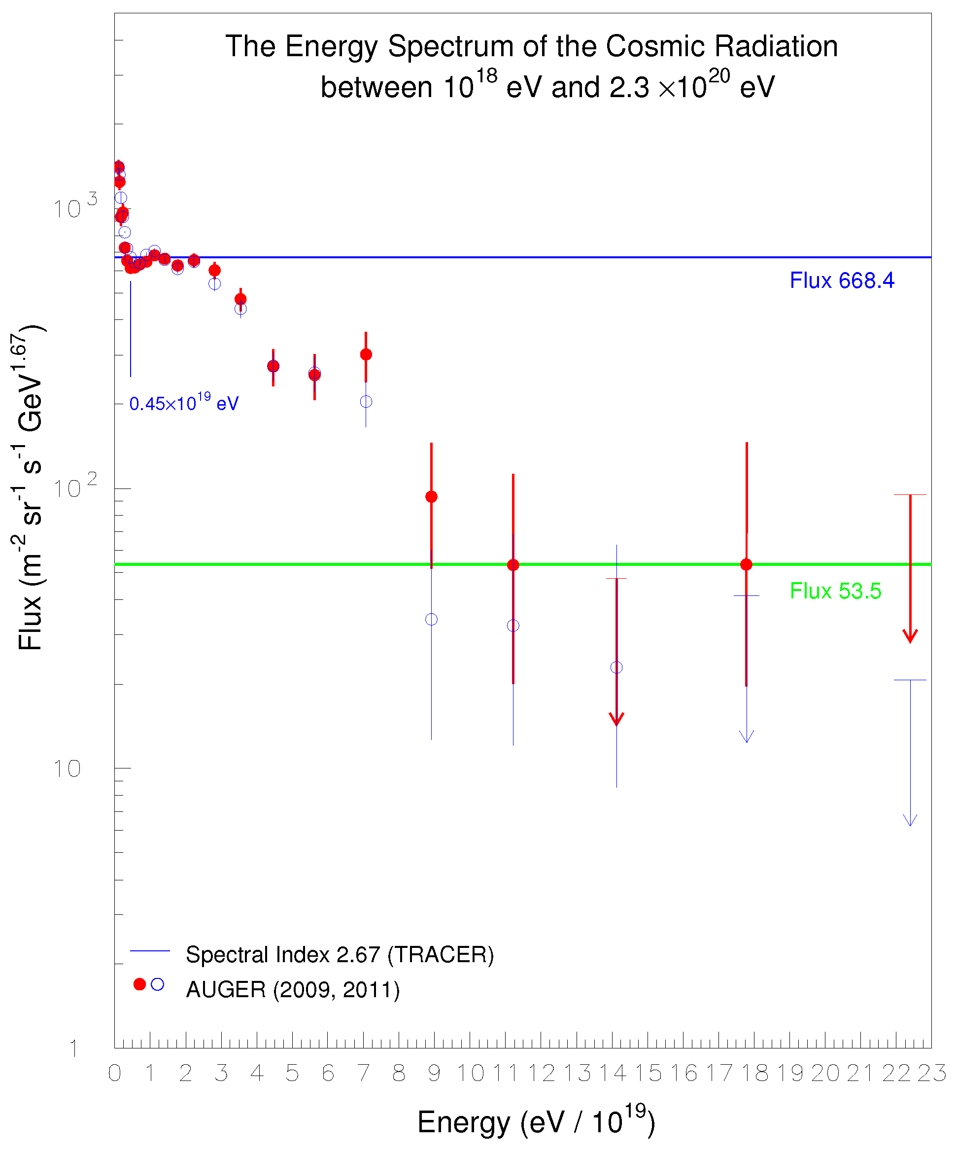
The break in the energy spectrum represents a direct, solid and unmistakable support to the present evaluation of the electrostatic potentials. It is direct because, given the electrostatic potential V(r), the energy achieved by cosmic-ray nuclei of atomic number Z is just ZqV as detailed above. It is solid because the break [12,15] has been reconfirmed by the Telescope Array collaboration [16]. It is unmistakable because the Telescope Array collaboration [16]. It is unmistakable because cosmic-ray Helium of charge 2q produces a second break in the spectrum exactly where expected, namely, at the energy of ( ) = as displayed in Figure 14 (on this issue see 13, Section in [8]).
In this and other works [1,8,18,21] the observation of the spectral break at is regarded as a major discovery in in the last half century but neither the discoverers (the HiRes, Auger and Telescope Array Collaborations) nor the presently prevailing cosmic-ray community recognized it as an effect of the electrostatic potential. The spectral break was erroneously ascribed to the effect [13,14] even if the stunning and unpredicted heavy chemical composition of the cosmic rays above [24,25] and the spectral break at (Figure 13) are blatantly inconsistent with the effect.
Closing this work it is proper to recognize and acknowledge its ultimate empirical foundation.
The negative electric charge, = - C from which the electric field partially originates, resides on the thin disk made of stars, molecular and atomic Hydrogen and heavier elements. As the negative charge rotates with the disk at about 240 /s, a Galactic magnetic field is generated (here labeled first component). The magnetic field strength resulting from the rotating charge is about 1 G [1,8] in agreement with the reiterated measurements of about 1 G performed during half a century by optical [26,27] and radio astronomers [28,29,30,31].
In addition to the first component, the circulation of cosmic-ray particles through the Galaxy (see Section 1) generates a second component of the magnetic field of about 1 G derived elsewhere (see 14 and 15 of ref. [8]). The derivation is simple but lengthy3.
Adding the first component (rotating electric charge stored in the Galactic disk) to the second component (cosmic-ray circulation), the strength and magnetic filed line pattern (geometry) of the global, regular, Galactic magnetic field is obtained. The accordance of the magnetic field strength and its geometry with observations, due to its unique and variegated signature, is the ultimate empirical foundation the electrostatic field and of this work4.
Conflicts of Interest
The author declare no conflicts of interest.
Appendix A. Numerical Values of Electric Fields and Related Potentials
The charge distributions of 3 and 4 have cylindrical forms. In this case, unlike the formulae derived analytically from , the electric fields and potentials have been calculated by a numerical method. The volume occupied by electric charge = - C is subdivided in half million small subvolumes each storing subcharges proportional to the subvolumes and the global electrostatic field is calculated by adding together all the subcharge elements. The method is cross-checked by structures where analytical formulae are available from classical . In this A some numerical data sets of electric fields of 4 are reported. The radial field profiles E(r,0) shown in Figure 8 (blue curves) for = 1, 2 and 3 are reported in Table A1. Table A2 reports the electrostatic potential versus elevation z of Model 4 for the positive charged halo of cosmic rays = 1 kpc at the three radial distances r = 0, 8.5 and 12 kpc (data displayed in Figure 9). Table A3 reports the electrostatic potentials V(r, 0) at elevation z = 0 versus radial distance r of Model 4 for the three values = 1, 2 and 3 kpc of the positive charged halo of cosmic rays (data displayed in Figure 10).

Table A1.
Electric field in V/m versus radius r of Model 4 in the range 1.5 ≤ r ≤ 18 kpc for three values of the positive charged halo of the cosmic rays = 1,2 and 3 kpc.
Table A1.
Electric field in V/m versus radius r of Model 4 in the range 1.5 ≤ r ≤ 18 kpc for three values of the positive charged halo of the cosmic rays = 1,2 and 3 kpc.
| r (kpc) | = 1 kpc | = 2 kpc | = 3 kpc |
|---|---|---|---|
| 1.5 | -0.041 | -0.0462 | -0.049550 |
| 2.0 | -0.068 | -0.0769 | -0.081620 |
| 2.5 | -0.078 | -0.0881 | -0.094085 |
| 3.0 | -0.079 | -0.0917 | -0.098739 |
| 3.5 | -0.078 | -0.0927 | -0.010104 |
| 4.0 | -0.07 | -0.0934 | -0.010274 |
| 4.5 | -0.07 | -0.0935 | -0.010450 |
| 5.0 | -0.07 | -0.0937 | -0.010603 |
| 5.5 | -0.07 | -0.0937 | -0.010765 |
| 6.0 | -0.06 | -0.0941 | -0.010966 |
| 6.5 | -0.06 | -0.0940 | -0.011160 |
| 7.0 | -0.060 | -0.0942 | -0.011394 |
| 7.5 | -0.068 | -0.0945 | -0.011667 |
| 8.0 | -0.060 | -0.0955 | -0.011994 |
| 8.5 | -0.057 | -0.0952 | -0.012391 |
| 9.0 | -0.056 | -0.098 | -0.012930 |
| 9.5 | -0.055 | -0.100 | -0.013592 |
| 10.0 | -0.055 | -0.103 | -0.014446 |
| 10.5 | -0.054 | -0.107 | -0.015550 |
| 11.0 | -0.054 | -0.114 | -0.017078 |
| 11.5 | -0.055 | -0.124 | -0.018169 |
| 12.0 | -0.058 | -0.139 | -0.022144 |
| 12.5 | -0.065 | -0.164 | -0.016623 |
| 13.0 | -0.075 | -0.202 | -0.033278 |
| 13.5 | -0.097 | -0.268 | -0.043612 |
| 14.0 | -0.0136 | -0.371 | -0.058729 |
| 14.5 | -0.0190 | -0.498 | -0.075920 |
| 15.0 | -0.0210 | -0.543 | -0.081864 |
| 15.5 | -0.015 | -0.434 | -0.067690 |
| 16.0 | -0.095 | -0.286 | -0.047475 |
| 16.5 | -0.056 | -0.182 | -0.032094 |
| 17.0 | -0.035 | -0.119 | -0.022114 |
| 17.5 | -0.022 | -0.081 | -0.015702 |
| 18.0 | -0.016 | -0.058 | -0.011569 |
Table A2.
Electrostatic potential in units of V versus elevation z of Model 4 for the positive charged halo of cosmic rays = 1 kpc at the three radial distances r = 0, 8.5 and 12 kpc (data displayed in Figure 9).
Table A2.
Electrostatic potential in units of V versus elevation z of Model 4 for the positive charged halo of cosmic rays = 1 kpc at the three radial distances r = 0, 8.5 and 12 kpc (data displayed in Figure 9).
| z (pc) | r = 0 | r = 8.5 kpc | r = 12 kpc |
|---|---|---|---|
| 0 | -4.14 | -1.93380 | -2.51648 |
| 10 | -4.13 | -1.93335 | -2.51510 |
| 50 | -4.03 | -1.9256 | -2.50568 |
| 150 | -3.74 | -1.8997 | -2.45787 |
| 150 | -3.37 | -1.8560 | -2.38254 |
| 200 | -2.96 | -1.7949 | -2.28018 |
| 250 | -2.57 | -1.7252 | -2.15665 |
| 300 | -2.21 | -1.6466 | -2.01585 |
| 350 | -1.88 | -1.5564 | -1.86311 |
| 400 | -1.59 | -1.4552 | -1.70035 |
| 450 | -1.34 | -1.3441 | -1.53425 |
| 500 | -1.12 | -1.2324 | -1.38299 |
| 600 | -0.732 | -1.0091 | -1.05266 |
| 700 | -0.437 | -0.79123 | -0.76435 |
| 800 | -0.218 | -0.59810 | -0.52876 |
| 900 | -0.11 | -0.434008 | -0.33320 |
| 1000 | -0.045 | -0.289041 | -0.192228 |
| 1100 | -0.029 | -0.17583 | -0.085085 |
| 1200 | -0.021 | -0.085482 | -0.0054361 |
| 1300 | -0.021 | -0.010932 | 0.0478883 |
Table A3.
Electrostatic potentials V(r, 0) at elevation z = 0 in units of V versus radial distance r of Model 4 for the three values = 1, 2 and 3 kpc of the positive charged halo of cosmic rays (data displayed in Figure 10).
Table A3.
Electrostatic potentials V(r, 0) at elevation z = 0 in units of V versus radial distance r of Model 4 for the three values = 1, 2 and 3 kpc of the positive charged halo of cosmic rays (data displayed in Figure 10).
| r (kpc) | z = 1 kpc | z = 2 kpc | z = 3 kpc |
|---|---|---|---|
| 0.0 | -4.138 | -8.510 | -12.794 |
| 0.5 | -3.996 | -8.576 | -12.919 |
| 1.0 | -3.995 | -8.544 | -12.290 |
| 1.5 | -3.949 | -8.490 | -12.841 |
| 2.0 | -3.890 | -8.431 | -12.769 |
| 2.5 | -3.807 | -8.313 | -12.656 |
| 3.0 | -3.696 | -8.183 | -12.510 |
| 3.5 | -3.575 | -8.051 | -12.366 |
| 4.0 | -3.472 | -8.945 | -12.239 |
| 4.5 | -3.351 | -7.788 | -12.072 |
| 5.0 | -3.230 | -7.636 | -11.894 |
| 5.5 | -3.112 | -7.502 | -11.748 |
| 6.0 | -3.016 | -7.362 | -11.602 |
| 6.5 | -2.890 | -7.206 | -11.407 |
| 7.0 | -2.786 | -7.049 | -11.215 |
| 7.5 | -2.718 | -6.926 | -11.070 |
| 8.0 | -2.605 | -6.761 | -10.857 |
| 8.5 | -2.516 | -6.626 | -10.687 |
| 9.0 | -2.441 | -6.496 | -10.503 |
| 9.5 | -2.357 | -6.326 | -10.284 |
| 10.0 | -2.259 | -6.167 | -10.073 |
| 10.5 | -2.174 | -6.006 | -9.838 |
| 11.0 | -2.094 | -5.844 | -9.598 |
| 11.5 | -2.014 | -5.654 | -9.309 |
| 12.0 | -1.933 | -5.451 | -8.998 |
| 12.5 | -1.830 | -5.222 | -8.627 |
| 13.0 | -1.726 | -4.948 | -8.174 |
| 13.5 | -1.600 | -4.588 | -7.584 |
| 14.0 | -1.424 | -4.093 | -6.788 |
| 14.5 | -1.163 | -3.415 | -5.742 |
| 15.0 | -0.844 | -2.588 | -4.494 |
| 15.5 | -0.567 | -1.840 | -3.340 |
| 16.0 | -0.366 | -1.282 | -2.454 |
References
- Codino, A. The ubiquitous mechanism accelerating cosmic rays at all the energies. In Proceedings of the 37th International Cosmic Ray Conference, 2022, p. 450, [arXiv:astro-ph.HE/2109.04388]. [CrossRef]
- DAMPE Collaboration.; Ambrosi, G.; An, Q.; Asfandiyarov, R.; Azzarello, P.; Bernardini, P.; Bertucci, B.; Cai, M.S.; Chang, J.; Chen, D.Y.; et al. Direct detection of a break in the teraelectronvolt cosmic-ray spectrum of electrons and positrons. 2017, 552, 63–66. [CrossRef]
- Abdollahi, S.; Ackermann, M.; Ajello, M.; Atwood, W.B.; Baldini, L.; Barbiellini, G.; Bastieri, D.; Bellazzini, R.; Bloom, E.D.; Bonino, R.; et al. Cosmic-ray electron-positron spectrum from 7 GeV to 2 TeV with the Fermi Large Area Telescope. Phys. Rev. D 2017, 95, 082007. [CrossRef]
- Beck, R.; Graeve, R. The distribution of thermal and nonthermal radio continuum emission of M31. 1982, 105, 192–199.
- Tabatabaei, F.S.; Schinnerer, E.; Murphy, E.; Beck, R.; Hughes, A.; Groves, B. The resolved radio-FIR correlation in nearby galaxies with Herschel and Spitzer. In Proceedings of the The Spectral Energy Distribution of Galaxies - SED 2011; Tuffs, R.J.; Popescu, C.C., Eds., 2012, Vol. 284, IAU Symposium, pp. 400–403, [arXiv:astro-ph.CO/1111.6252]. [CrossRef]
- Gajović, L.; Heesen, V.; Brüggen, M.; Edler, H.W.; Adebahr, B.; Pasini, T.; de Gasperin, F.; Basu, A.; Weżgowiec, M.; Horellou, C.; et al. The low-frequency flattening of the radio spectrum of giant H II regions in M 101. 2025, 695, A41, [arXiv:astro-ph.GA/2502.08713]. [CrossRef]
- Lozinskaya, T.A.; Kardashev, N.S. The Thickness of the Gas Disk of the Galaxy from 21-cm Observations. 1963, 7, 161.
- Codino, A. The ubiquitous mechanism accelerating cosmic rays at all the energies; Società editrice Esculapio: Bologna, Italy, 2020.Corrected reprint published in 2023.
- Jackson, P.D.; Kellman, S.A. A Redetermination of the Galactic H i Half-Thickness and a Discussion of Some Dynamical Consequences. 1974, 190, 53–58. [CrossRef]
- Voshage, H.; Feldmann, H.; Braun, O. Investigations of cosmic-ray-produced nuclides in iron meteorites: 5. More data on the nuclides of potassium and noble gases, on exposure ages and meteoroid sizes. Zeitschrift Naturforschung Teil A 1983, 38, 273–280. [CrossRef]
- Salamida, F. Update on the measurement of the CR energy spectrum above 10**18-eV made using the Pierre Auger Observatory. In Proceedings of the 32nd International Cosmic Ray Conference, 8 2011.
- Abraham, J.; Abreu, P.; Aglietta, M.; Aguirre, C.; Allard, D.; Allekotte, I.; Allen, J.; Allison, P.; Alvarez-Muñiz, J.; Ambrosio, M.; et al. Observation of the Suppression of the Flux of Cosmic Rays above 4 × 10¹⁹ eV. Phys. Rev. Lett. 2008, 101, 061101. [CrossRef]
- Greisen, K. End to the Cosmic-Ray Spectrum? 1966, 16, 748–750. [CrossRef]
- Zatsepin, G.T.; Kuz’min, V.A. Upper Limit of the Spectrum of Cosmic Rays. Soviet Journal of Experimental and Theoretical Physics Letters 1966, 4, 78.
- Abbasi, R.U.; Abu-Zayyad, T.; Allen, M.; Amman, J.F.; Archbold, G.; Belov, K.; Belz, J.W.; Ben Zvi, S.Y.; Bergman, D.R.; Blake, S.A.; et al. First Observation of the Greisen-Zatsepin-Kuzmin Suppression. Physical Review Letters 2008, 100, 101101, [astro-ph/0703099]. [CrossRef]
- Abu-Zayyad, T.; Aida, R.; Allen, M.; Anderson, R.; Azuma, R.; Barcikowski, E.; Belz, J.W.; Bergman, D.R.; Blake, S.A.; Cady, R.; et al. The Cosmic-Ray Energy Spectrum Observed with the Surface Detector of the Telescope Array Experiment. 2013, 768, L1, [arXiv:astro-ph.HE/1205.5067]. [CrossRef]
- Codino, A. About the consistency of the energy scales of past and present instruments detecting cosmic rays above the ankle energy. arXiv e-prints 2017, p. arXiv:1710.06659, [arXiv:astro-ph.HE/1710.06659]. https://doi.org/10.48550/arXiv.1710.06659. [CrossRef]
- Codino, A. The absence of the GZK depression in the energy spectrum of the cosmic radiation. In Proceedings of the 33rd International Cosmic Ray Conference, 2013, p. 0144.
- Codino, A. About the Energy Interval beyond the Ankle Where the Cosmic Radiation Consists Only of Ultraheavy Nuclei from Zinc to the Actinides. Journal of Applied Mathematics and Physics 2017, pp. 225–237. [CrossRef]
- Codino, A. The energy spectrum of ultraheavy nuclei above 1020 eV. Journal of Applied Mathematics and Physics 2017, pp. 1540–1550, [arXiv:astro-ph.HE/1707.02487]. [CrossRef]
- Codino, A. Redundant failures of the dip model of the extragalactic cosmic radiation. arXiv e-prints 2009, p. arXiv:0911.4273, [arXiv:astro-ph.HE/0911.4273]. https://doi.org/10.48550/arXiv.0911.4273. [CrossRef]
- Abraham, J.; Abreu, P.; Aglietta, M.; Ahn, E.J.; Allard, D.; Allen, J.; Alvarez-Muñiz, J.; Ambrosio, M.; Anchordoqui, L.; Andringa, S.; et al. Measurement of the energy spectrum of cosmic rays above 1018 eV using the Pierre Auger Observatory. Physics Letters B 2010, 685, 239–246, [arXiv:astro-ph.HE/1002.1975]. [CrossRef]
- Pierre Auger Collaboration. Measurement of the cosmic ray spectrum above 4 × 10¹⁸ eV using inclined events detected with the Pierre Auger Observatory. 2015, 2015, 049–049, [arXiv:astro-ph.HE/1503.07786]. [CrossRef]
- Unger, M.; Engel, R.; Schüssler, F.; Ulrich, R.; Pierre Auger Collaboration. Study of the Cosmic Ray Composition above 0.4 EeV using the Longitudinal Profiles of Showers observed at the Pierre Auger Observatory. Astronomische Nachrichten 2007, 328, 614, [arXiv:astro-ph/0706.1495]. [CrossRef]
- Abbasi, R.U.; Abe, M.; Abu-Zayyad, T.; Allen, M.; Anderson, R.; Azuma, R.; Barcikowski, E.; Belz, J.W.; Bergman, D.R.; Blake, S.A.; et al. Study of Ultra-High Energy Cosmic Ray composition using Telescope Array’s Middle Drum detector and surface array in hybrid mode. Astroparticle Physics 2015, 64, 49–62, [arXiv:astro-ph.HE/1408.1726]. [CrossRef]
- Mathewson, D.S.; Ford, V.L. Polarization observations of 1800 stars. 1971, 153, 525. [CrossRef]
- Jones, R.V.; Spitzer, Jr., L. Magnetic Alignment of Interstellar Grains. 1967, 147, 943. [CrossRef]
- Han, J.L.; Qiao, G.J. The magnetic field in the disk of our Galaxy. 1994, 288, 759–772.
- Rand, R.J.; Kulkarni, S.R. The Local Galactic Magnetic Field. 1989, 343, 760. [CrossRef]
- Rand, R.J.; Lyne, A.G. New Rotation Measures of Distant Pulsars in the Inner Galaxy and Magnetic Field Reversals. 1994, 268, 497. [CrossRef]
- Mitra, D.; Wielebinski, R.; Kramer, M.; Jessner, A. The effect of HII regions on rotation measure of pulsars. 2003, 398, 993–1005. [CrossRef]
| 1 | Consider two equal masses m retaining the same electric charge q (see Figure 1 in [7]. They experience an electrostatic repulsion and, at the same time, a gravity pull. Equilibrium or balance between the two forces occurs when the charge-to-mass ratio is q/m = = C/ where = F/m and G = 42 /. The definition of balance charge ( the subscript b is for balance) is, ≡m and, in turn, ζ≡q/. The dimensionless variable ζ as charge unit is devoid of any subtlety, just a definition. For example, the balance charge of the is M = C where M = is an arbitrary mass adopted in works [1,8] and others. |
| 2 | For simplicity it is admitted that in the propagation of cosmic rays the particle density from the emitting source depends on the distance r as 1/r up to a characteristic distance R. This behavior is ascribed to the chaotic components of the magnetic field around the source. |
| 3 | The traditional concepts of Cosmic Ray Physics as freezed in textbooks and articles in top reviews are inane to determine the geometry of the regular magnetic field. In fact traditional concepts adopt the diffusive propagation of cosmic rays which do not form current loops in the Galaxy. As the diffusive propagation occurs in magnetic fields and ignores the Galactic electrostatic field, it is detached from the physical reality of the as proved by plenty of measurements. |
| 4 | This work is dedicated to Livia Chiavaroli Codino. |
Figure 1.
Qualitative illustration of the positions of the electric charges transported by cosmic rays in a spherical globe of maximum size . The negative charges of the electrons of the quiescent galactic matter are represented by negative signs and they are confined in a region of size 2 while the positive charges of protons, nuclei and positrons represented by plus signs extend up to . High energy electrons, unlike protons and nuclei, radiate synchrotron (curvature) light and cannot diffuse over large distances from the globe of characteristic size 2. Cosmic nuclei propagate via a diffusive-alternate motion forming a halo of positive charge whose density decreases with the radial distance r in the range 0 ≤r≤R. The different distributions of the negative (quiescent electrons) and positive (cosmic nuclei) charges generate an electrostatic field denoted . The cartoon is not at scale and ignores many details discussed elsewhere.
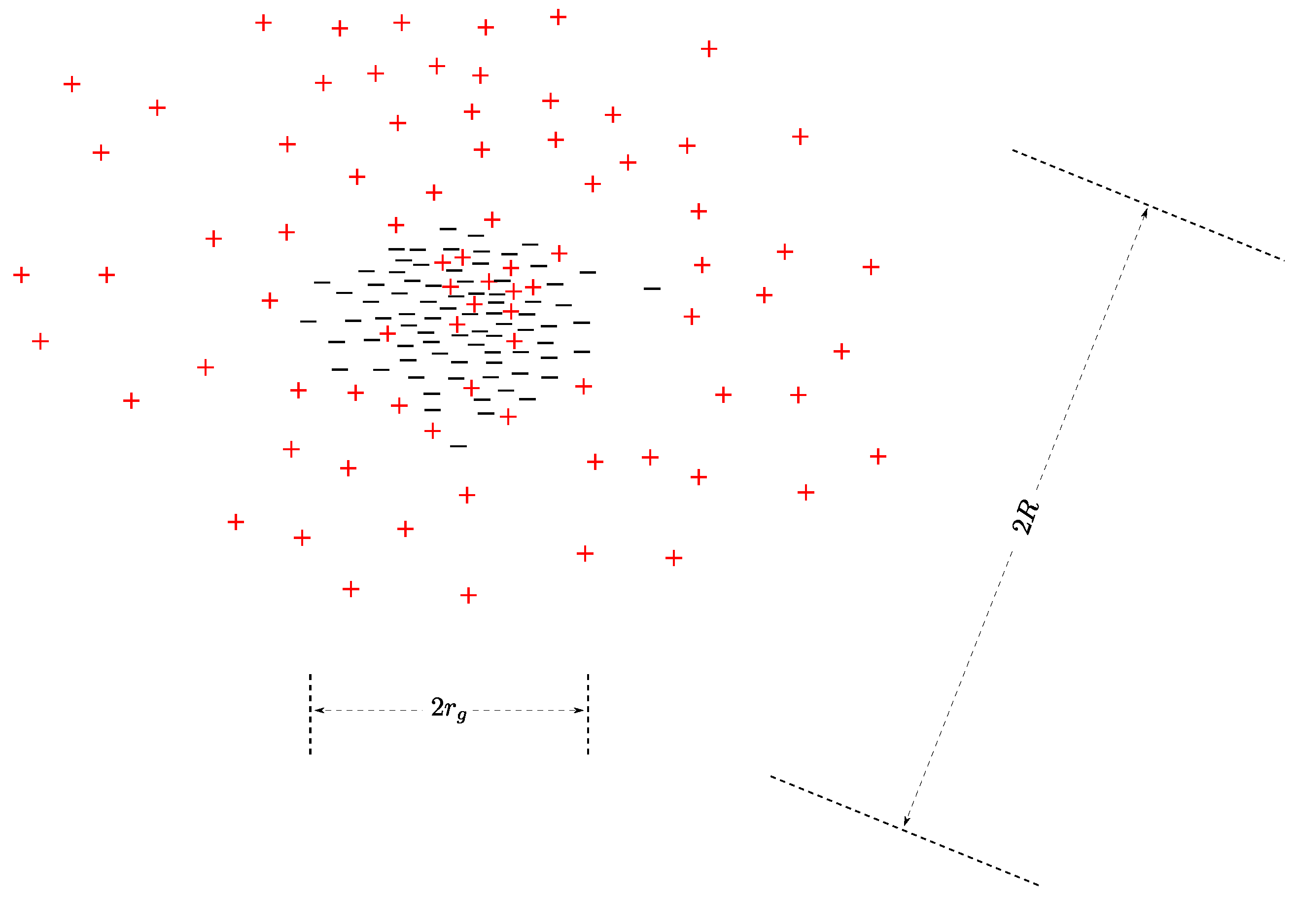
Figure 2.
Geometrical forms of the electric charge distributions of the five models imitating the electric charge in very large volumes of galactic dimension. Model 1 (Figure 2-a) are the double, concentric spheres with constant charge densities. Model 2 consists of two concentric spheres: a uniformly negatively charged sphere surrounded by a positively charged spherical halo with decreasing density from the center (Figure 2-b). Model 3 has the negative charge distributed in a flat disk of volume 2 h where h is the half thickness of the disk and its radius (Figure 2-c) while the positive charge is spherically distributed like model 2. Model 4 (Figure 2-d) consists of two highly squashed, concentric cylinders with the same radius and different heights, h and (the subscript h for halo of positive charge). Model 5 consists of six discrete pointlike negative charges /6 surrounded by a sphere of positive charge placed in a volume of galactic dimension.
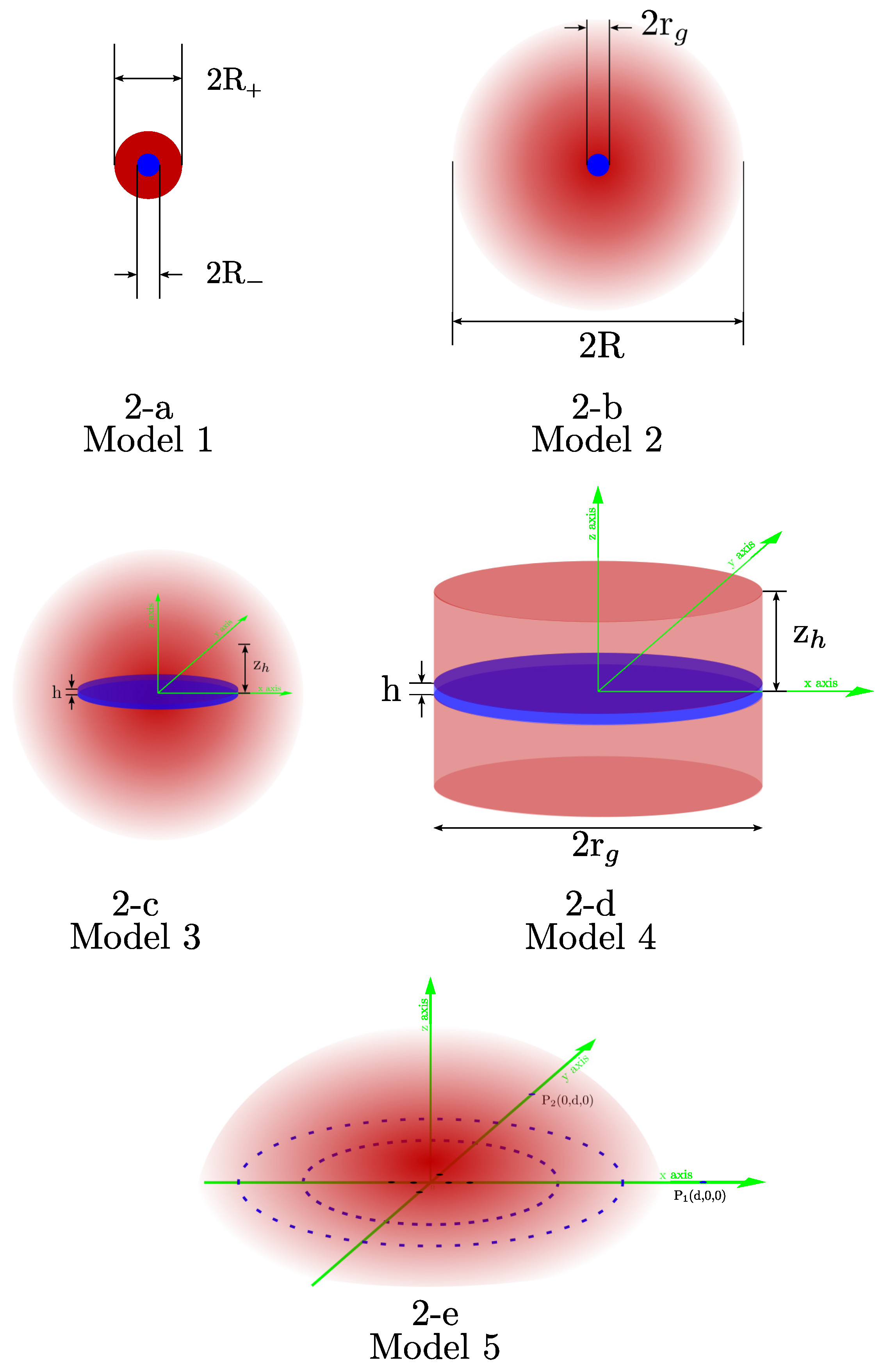
Figure 3.
Electric field intensity versus radius r of two spherical, concentric distributions of positive and negative electric charge contained within the sphere radii and , respectively. The results shown here arbitrarily adopts, = - = C, = 5 , = 3 = 15 . The electric field is centripetal in the entire radial range, 0 ≤r≤. Figure 3-b Electrostatic potentials corresponding to the electric fields shown in Figure 3-a.
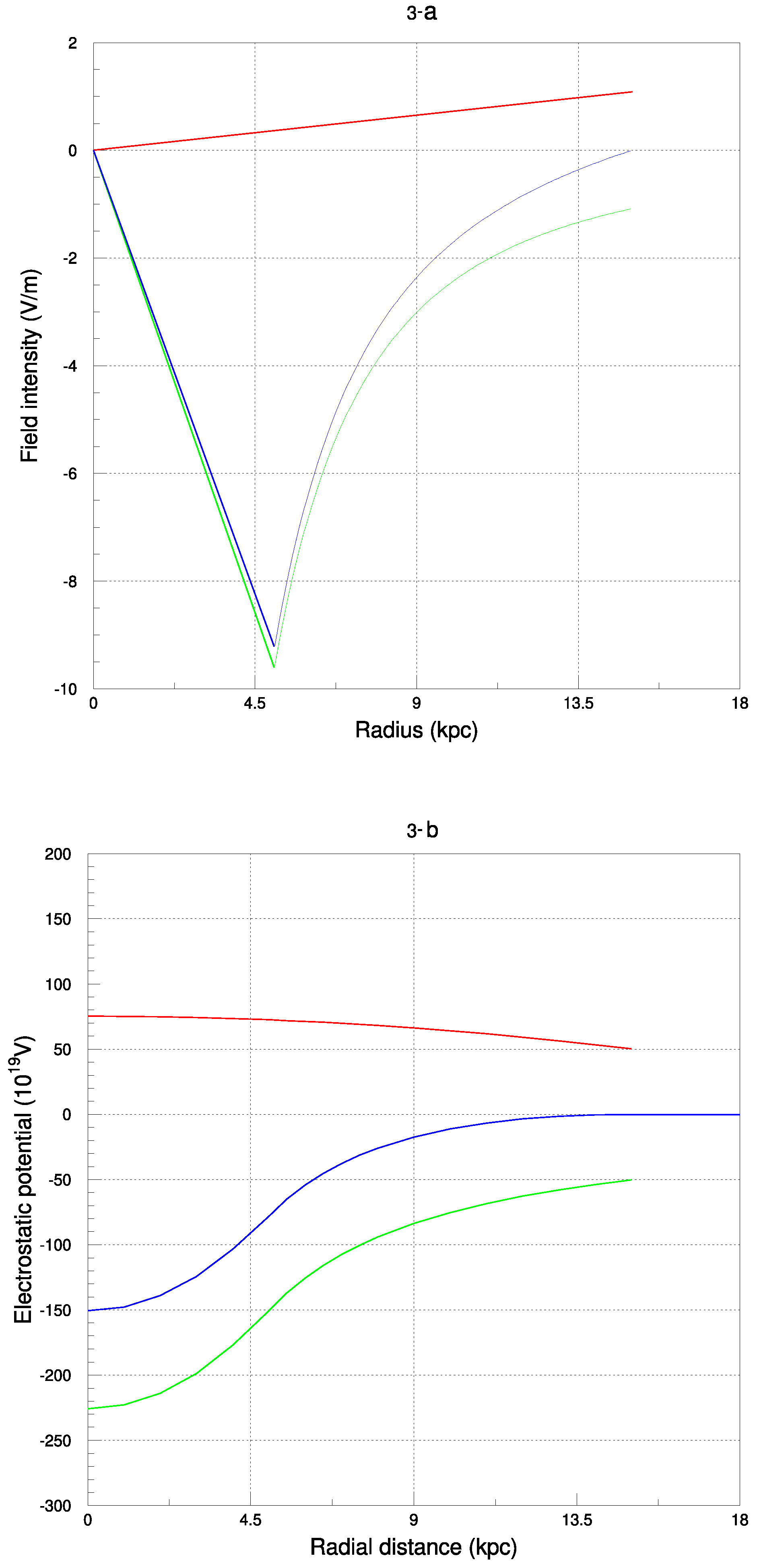
Figure 4.
Electrostatic field intensity (blue curve) versus radial distance r of a spherical volume with center and radius = 15 storing a uniform distribution of negative electric charge overlapped with a halo of positive charge distributed as (r) = k/r with k constant. The halo extends from the center up to the maximum distance of 300 . The electric field is generated by the charge and of ±C. The intensity of the field (r) produced by the sole positive charge (red curve) and the intensity of (r) produced by the sole negative charge (green charge) are also shown. The maximum field intensity is V/m at = 15 .
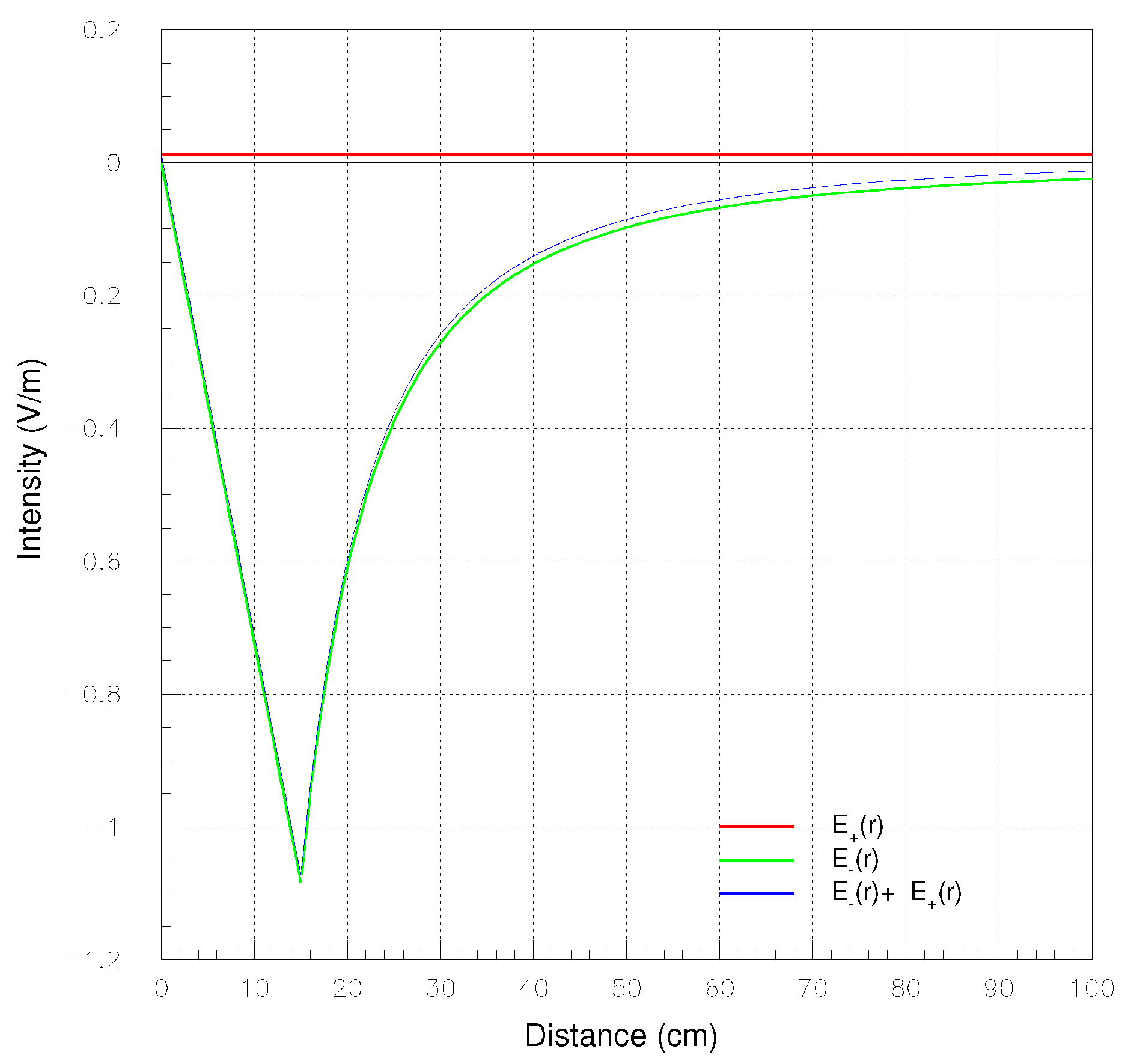
Figure 5.
Electrostatic potential versus elevation z (green curve) and radial distance (blue curve) are displayed. These profiles correspond to the electrostatic field represented in Figure 3 of a disk of negative charge immersed in a spherical halo of positive charge constrained by: = - = C. The maximum depth of this potential is -V. For comparison the potential of the double sphere with zero charge (grey curve), which has a maximum depth of -V is also shown.
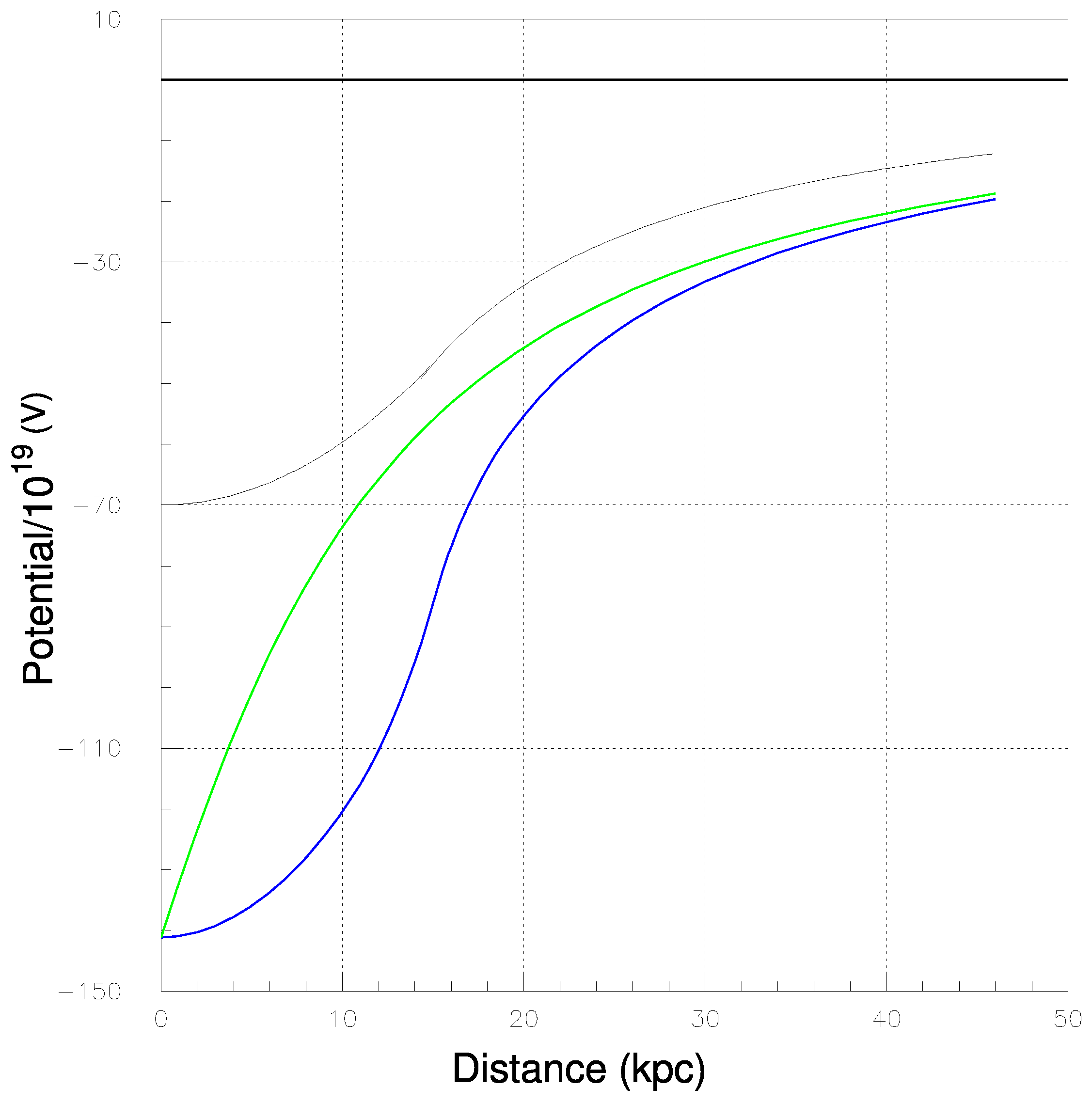
Figure 6.
Profiles of the electrostatic field in a disk imbued by the negative charge, = -C uniformly distributed within the volume 2h where it is overlapped an equal amount of positive electric charge, = - radially distributed as (r) = k/ r with k constant up to the maximum distance = 300 . 6-a Radial profile of the electric field (green curve) and elevation profile of the field per r = 0 (red curve) in the range, 0 <r< 25 . 6-b Profile of the electric field in elevation z in the interval, 0 <z< 250 for 4 radial distances: r = 0, r = , r = e r = . The trend of for r = 0 (red curve) is the continuation at small radial distances of the trend in Figure 6-a . Notice that distance scales in Figure 6-a and Figure 6-b are different while those of the field intensities are equal.
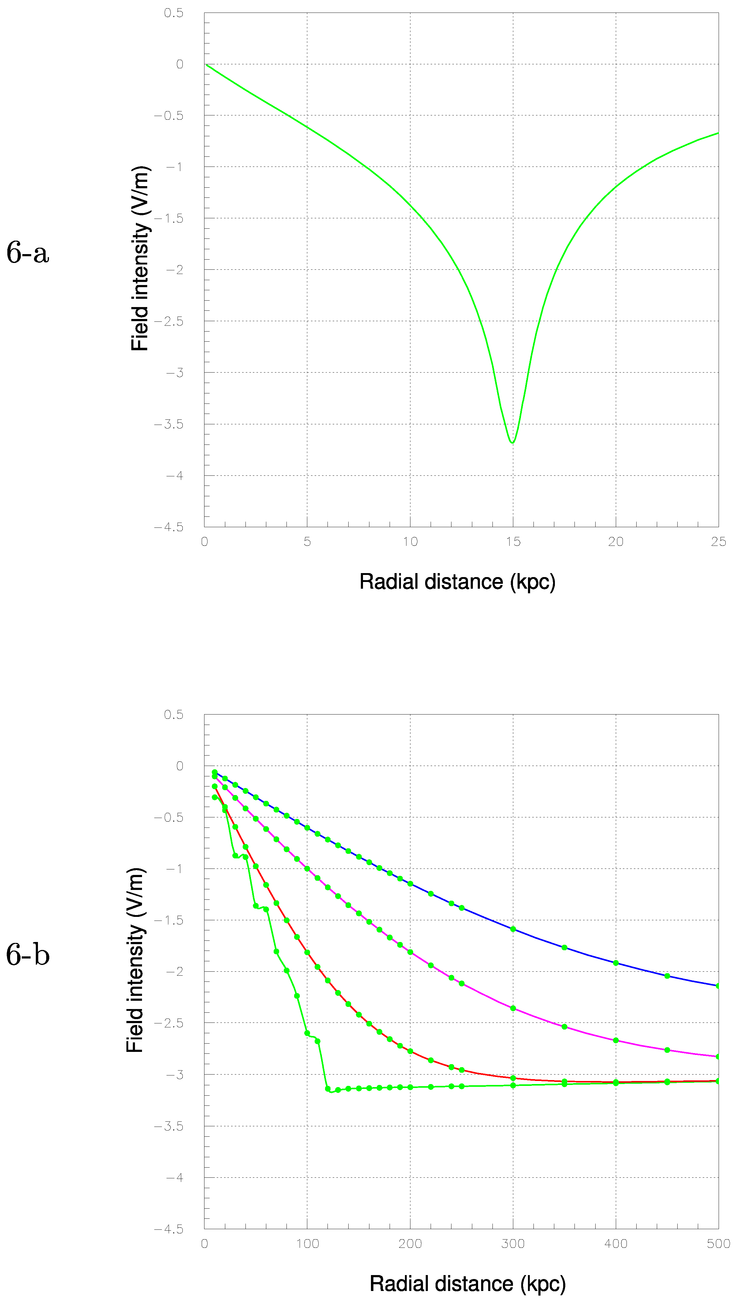
Figure 7.
Representation of the electrostatic field of the Milky Way Galaxy onto the plane xz for y = 0 using a vector array in the domain, 0 <x< 14 and -125 <z< 125 . The Galactic center (green dot) and the nominal position of the solar system (red dot) = and = 0 are shown. Note that distance scales are different: in the x axis they are kiloparsec, in the z axis . Around the center the inversion of the direction ( see Figure 19 ref. [8]) is ignored e. g. it is not visible.
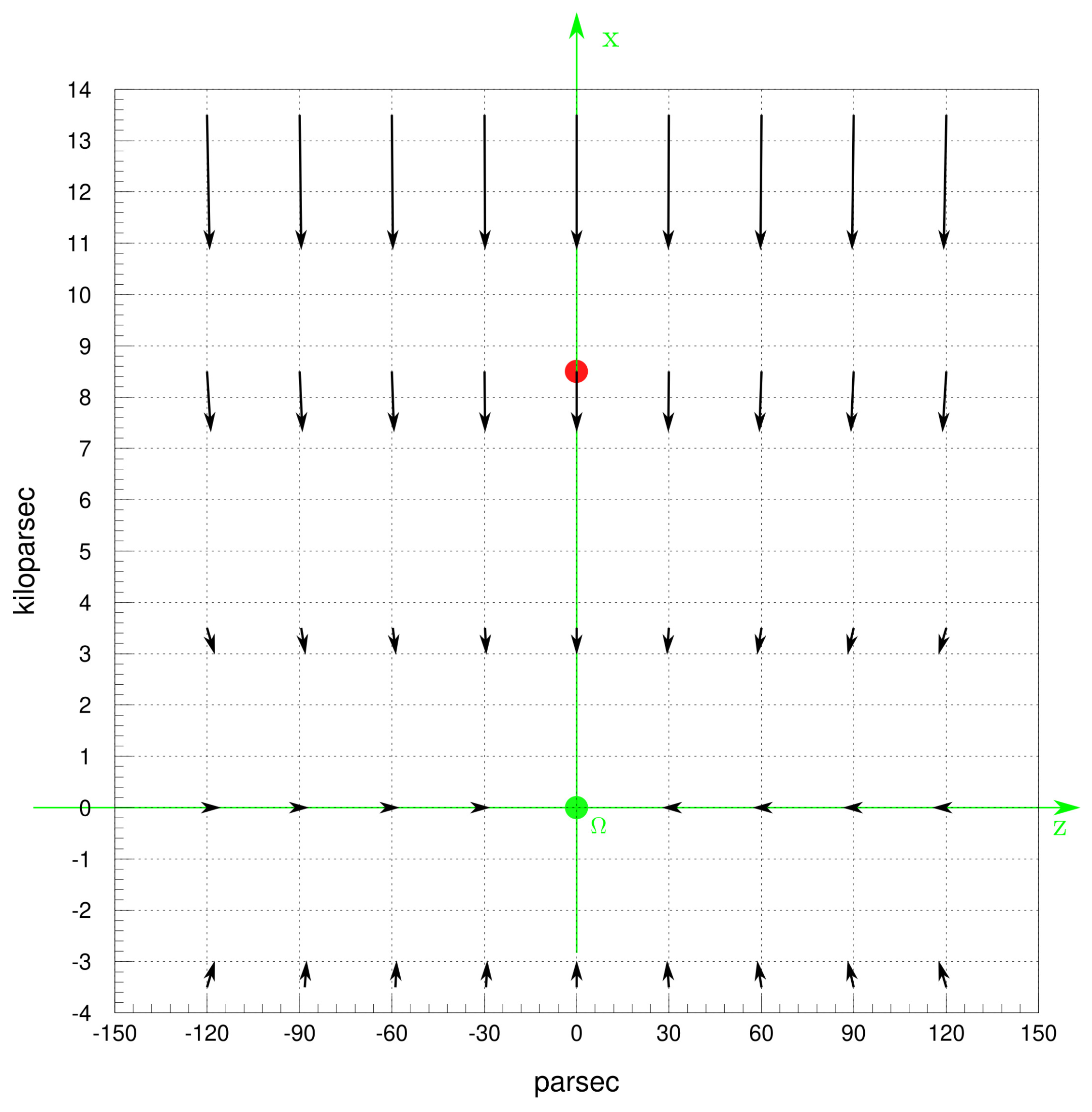
Figure 8.
Electric field intensity versus radial distance r for the Milky Way Galaxy obtained with two concentric, highly squashed cylindrical charge distributions. The negative charge has a radius of 15 and elevation (normal direction to the Galactic midplane) of 125 reflecting the location of cosmic-ray sources embedded in the molecular and atomic clouds. The positive charge has the same radius of 15 and a larger elevation of 2 reflecting the vast spread of cosmic-ray nuclei due to their abnormal high energies. Negative charge is = C and is equal to the positive charge.
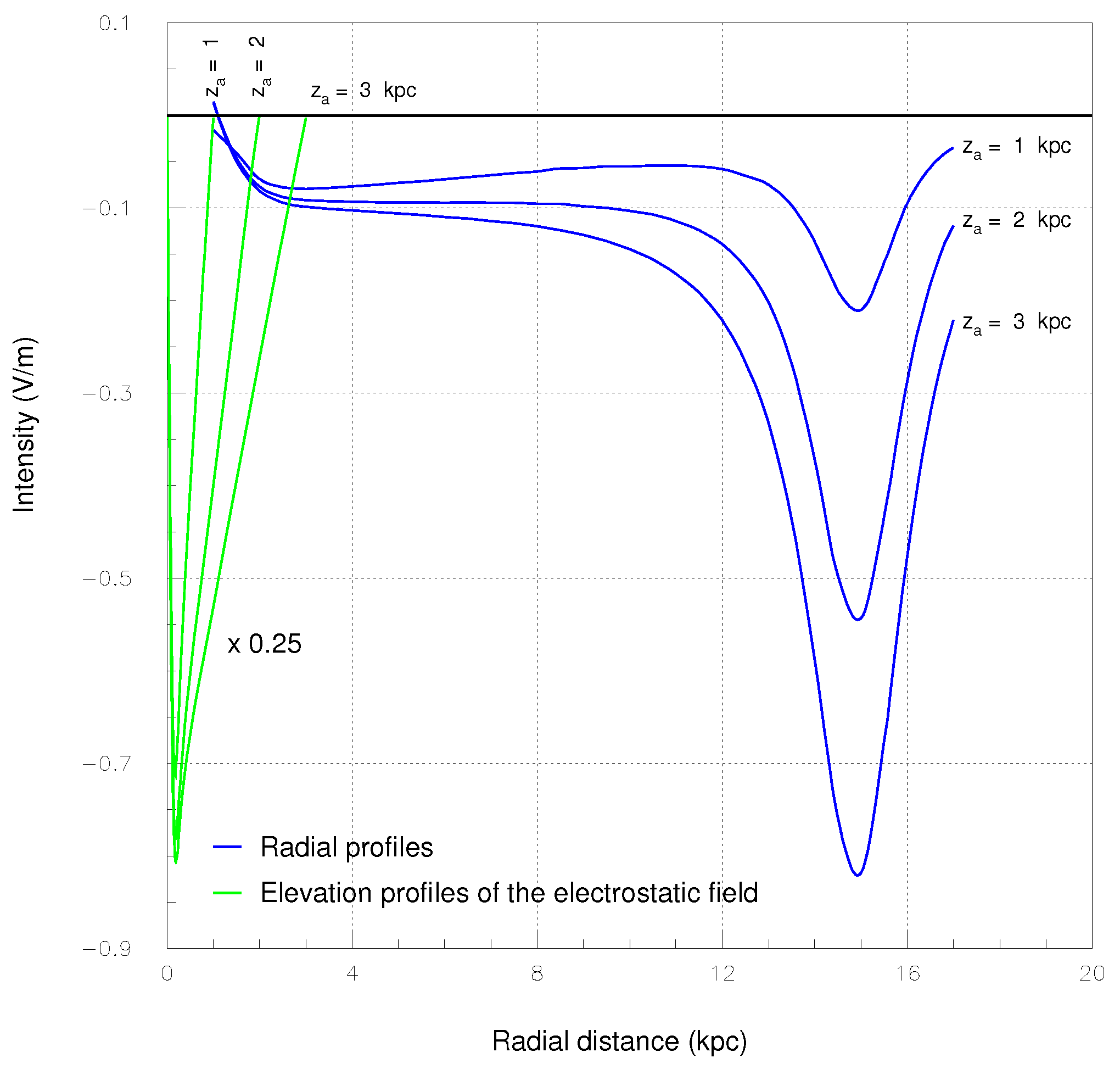
Figure 9.
Electrostatic potentials V(,z), V(,z) and V(,z) in elevation z at the three arbitrary radial distances = 0, = and =12 for the halo size = 1 . These potentials, in units of V, correspond to the electric field intensities (0,z) reported in Figure 9 (green curves).
Figure 9.
Electrostatic potentials V(,z), V(,z) and V(,z) in elevation z at the three arbitrary radial distances = 0, = and =12 for the halo size = 1 . These potentials, in units of V, correspond to the electric field intensities (0,z) reported in Figure 9 (green curves).
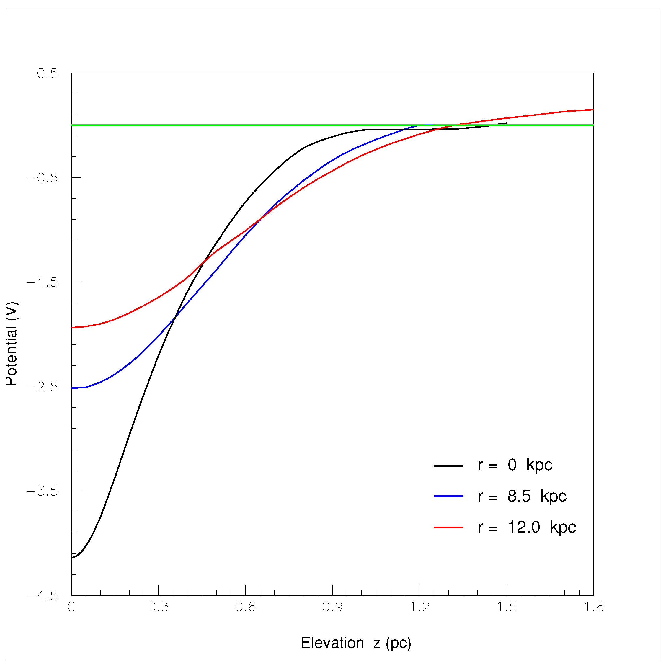
Figure 10.
Radial electrostatic potentials V(r,0) for three halo sizes = 1, 2 and 3 at the arbitrary elevation z = 0 (Galactic midplane). These potentials correspond to the electric fields (0,z) depicted in Figure 8 (blue curves). The two oblique black curves visualize the departure of the electrostatic potential from a linear extrapolation rooted in the radial range 4-8 (for = 3 and = 2 ).
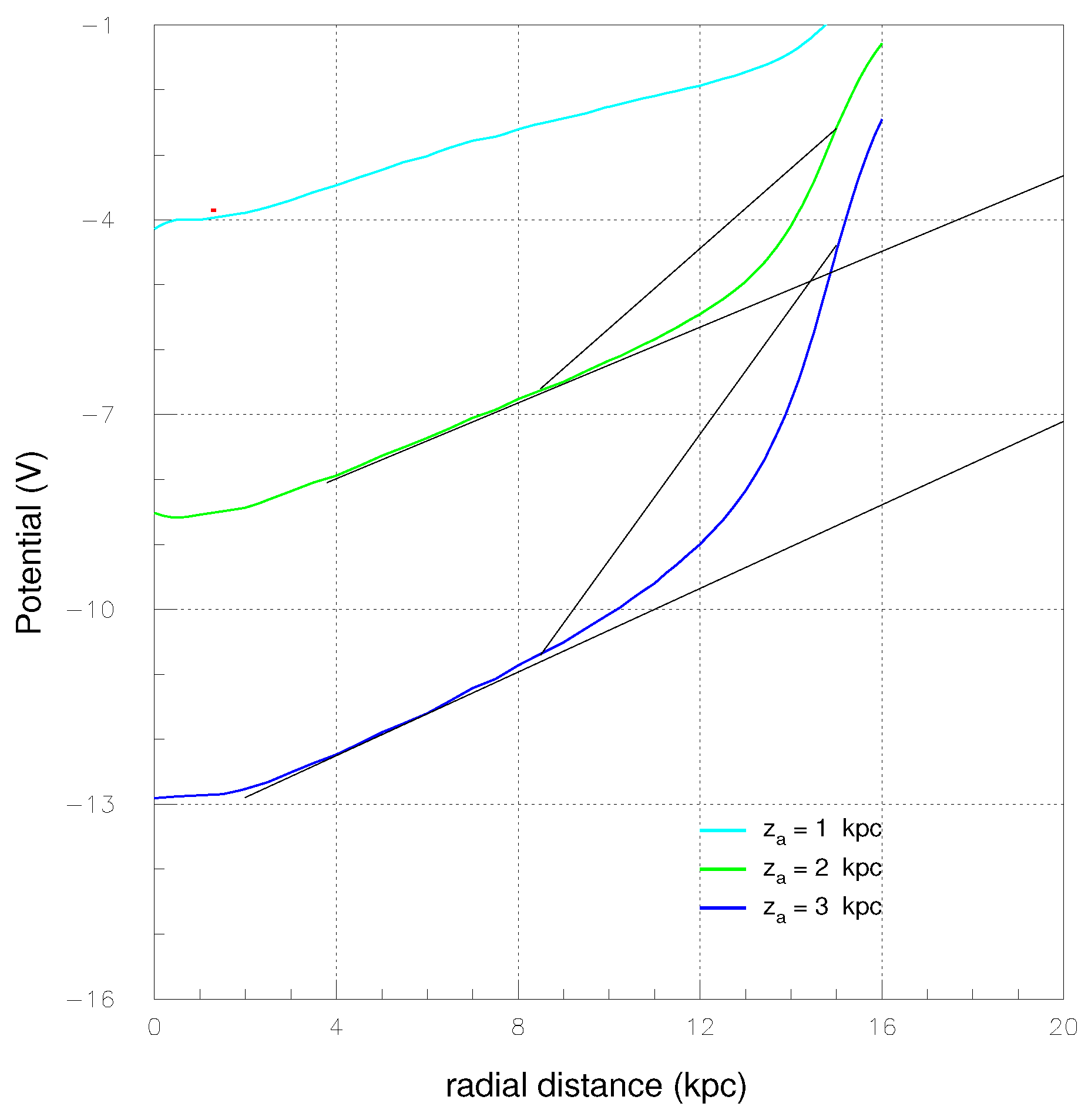
Figure 11.
The Galactic disk of two highly squashed cylinders incorporated in the calculation of the electrostatic potential still differs from fine astronomical observations. The disk enlargement at the extreme ends displayed in this figure (blue area) has been discovered in 1966 [7] and confirmed in the subsequent years (see, for example, ref. [9]). The negative charge dominates in the blue area (small cylinder of height h) while the positive charge dominates in the red area (large squashed red cylinder of height ) . The heights h and of the squashed cylinders are free parameters with typical values h = 125 and = 2 , respectively. The cylindrical geometry is a crude simplification of the real, complex pattern of matter distribution in the outer galaxy. The oblique position of the disk in this figure is arbitrary. These refinements may be useful to implement future, more precise calculations of the Galactic electrostatic field.
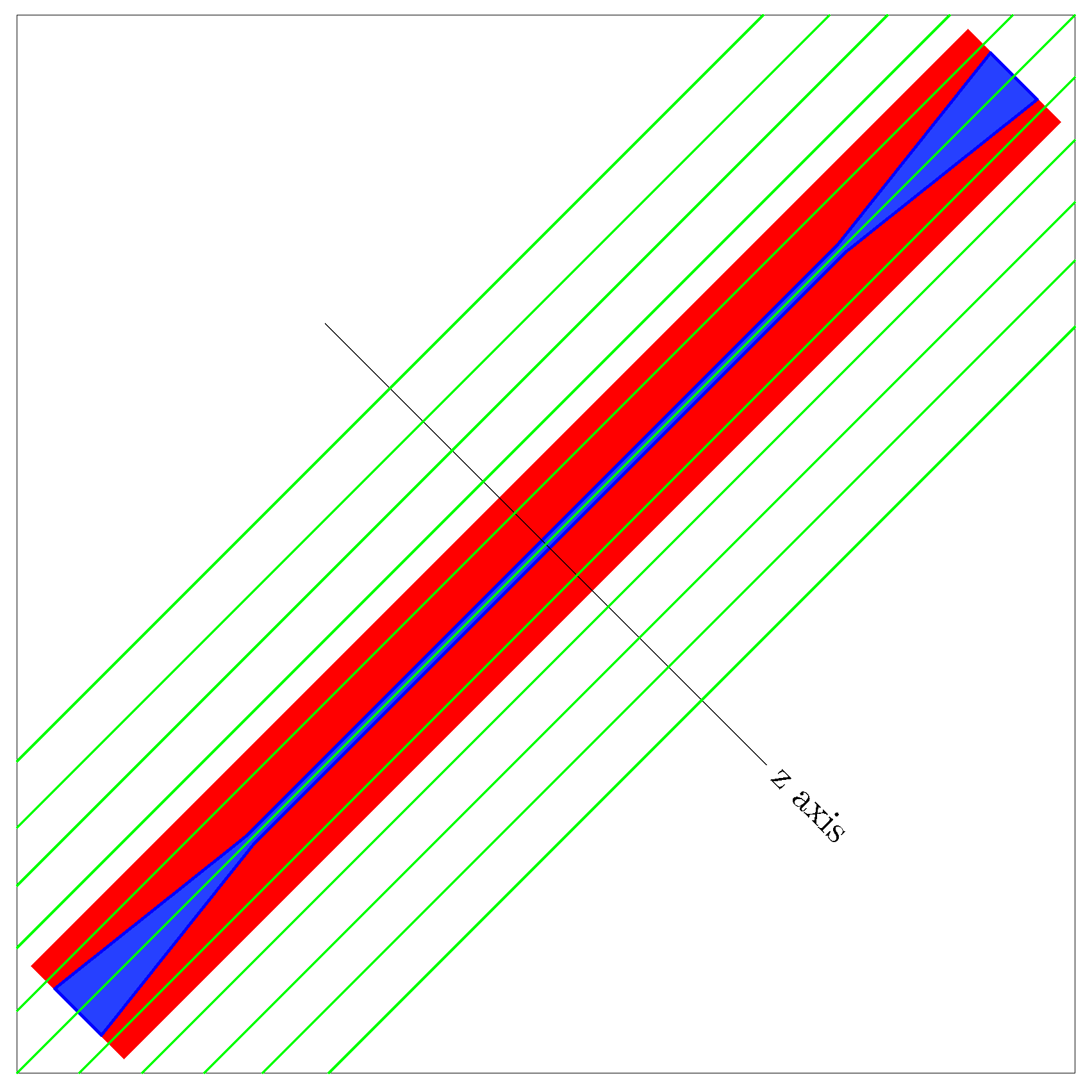
Figure 12.
On the pervasiveness of the galactic electrostatic fields. (12-a) An electrostatic system of six negative electric charges with total charge, = - C lie in a region of characteristic size 2a = 15 (central black dots). The six charges are immersed in a spherical halo of positive charge of radius R = 300 in such a manner that the total electric charge of the system is zero, e.g., = -. (12-b) Electrostatic field onto the xy plane represented by a vector array. Beyond the radius R (dashed circle) vectors are multiplied by a factor of 5 to render them visible. Generally the electric field extends over the entire cosmic space and does not vanish except in very restricted regions. A cosmic nucleus can travel from the point (d,0,0) to the point (0,d,0) across the potential well generated by the electrostatic system and abandon the well by a gain of energy. Anyone of these infinite number of paths is called .
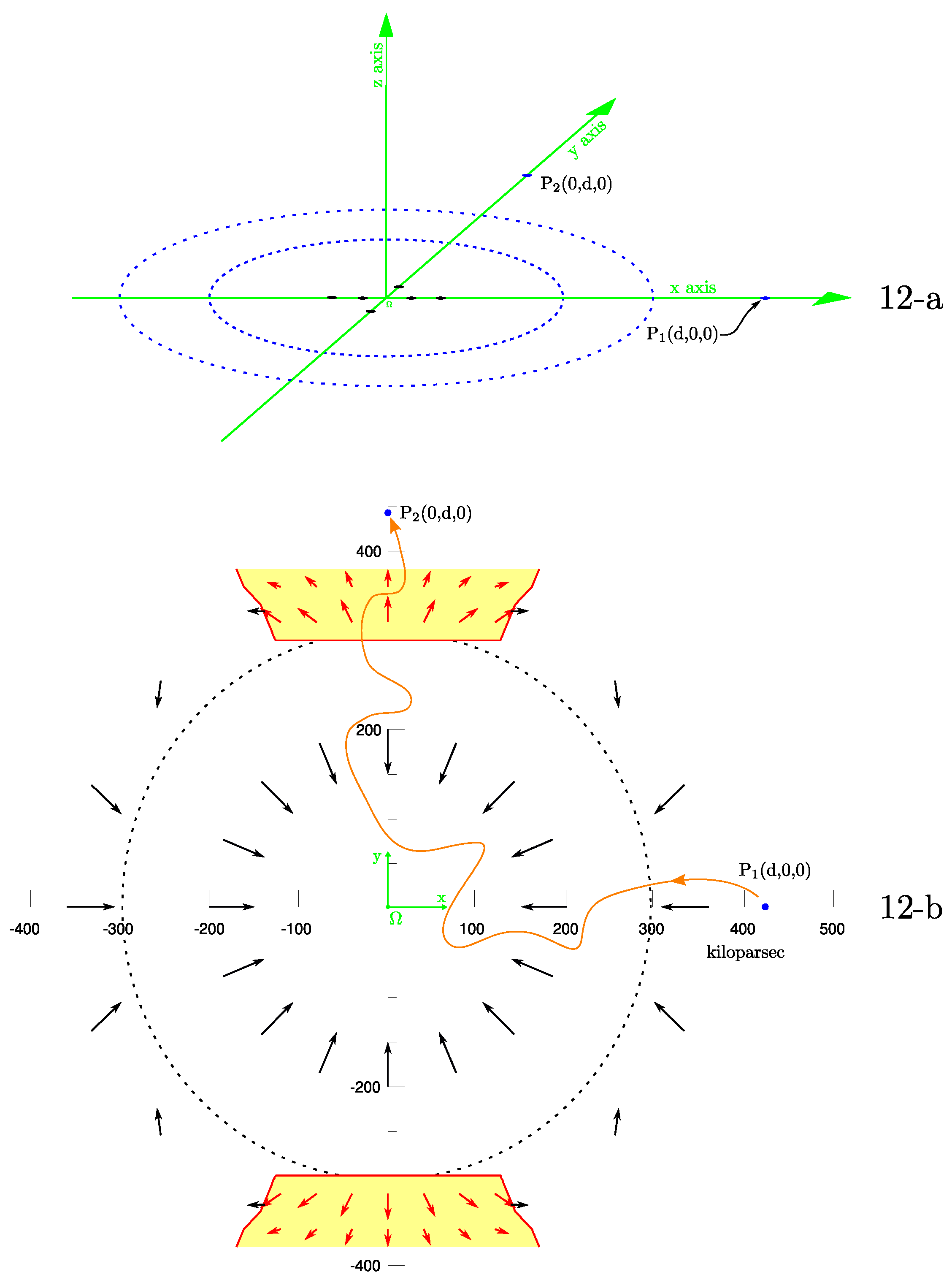
Figure 13.
Energy spectrum of cosmic rays in a linear scale of energy between and according to the data (red dots) of the [11]. The thin blue line, normalized to the value of /s at the arbitrary energy of , is an interpolation with the constant spectral index of the first 14 data points (red dots). The thick turquoise line is an interpolation of the last 4 data points in the range (2-5). The divarication of the measured spectrum (last 4 red dots) with that extrapolated with the index of 2.67 above the energy (blue curve) manifests in the energy band (2-3). The characteristic energy of the divarication, marks the lack of protons at the injection and pre-acceleration stages, shortly, a scarcity of protons at the sources. The unsurpassed statistical precision of the Auger experiment in the measurements of the energy spectrum [11] made possible the identification of the energy (the error bar in the last data point is barely visible).
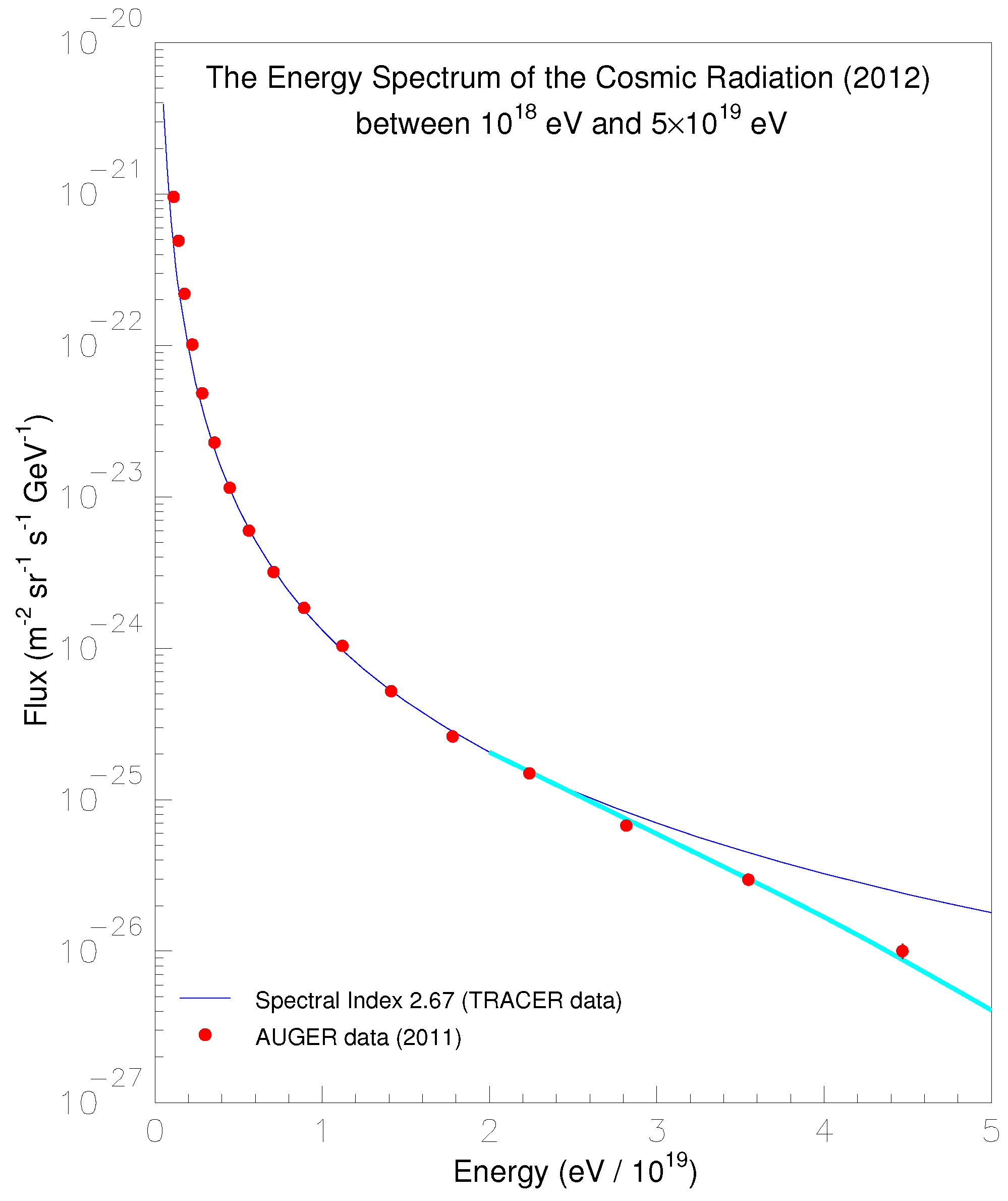
Figure 14.
Evidence for staircase drop of the cosmic ray spectrum above the energy based on the published data of the Auger experiment [11,22]. It is shown the quantity J(E) versus energy E which evidences the depletion of the cosmic-ray sources and, at the same time, reduces the effect of the spectral index as discussed in the text. The horizontal blue line represents the extrapolated flux with a spectral index = anchored to the data at energies lower than . The energy of reported in the figure is the particular energy where the measured spectrum [23] and that extrapolated coincide. It results: J()( = in the units shown; this position is a simple normalization to the data.
Disclaimer/Publisher’s Note: The statements, opinions and data contained in all publications are solely those of the individual author(s) and contributor(s) and not of MDPI and/or the editor(s). MDPI and/or the editor(s) disclaim responsibility for any injury to people or property resulting from any ideas, methods, instructions or products referred to in the content. |
© 2025 by the authors. Licensee MDPI, Basel, Switzerland. This article is an open access article distributed under the terms and conditions of the Creative Commons Attribution (CC BY) license (http://creativecommons.org/licenses/by/4.0/).
Copyright: This open access article is published under a Creative Commons CC BY 4.0 license, which permit the free download, distribution, and reuse, provided that the author and preprint are cited in any reuse.


