No–Inflation Under Pachner Moves for Teichmüller State–Integrals: A DSFL Residual Monotonicity Theorem

1. Introduction

This paper turns cutting and gluing stability in Teichmüller TQFT into a theorem: Pachner moves act as calibration–intertwining contractions in a single comparison Hilbert geometry, so any triangulation change provably cannot worsen a calibrated error; we quantify robustness, polarization angles and conditioning, recursion decay, and provide a practical certification framework.

Cutting and gluing lie at the heart of low–dimensional quantum topology and of state–integral realizations of Chern–Simons/Teichmüller TQFT [1,2,3,4]. In practice, computations based on ideal triangulations or exact recursion repeatedly replace one local presentation by another via Pachner moves [5]. What has been missing is a certifiable stability law ensuring that these rearrangements do not amplify numerical or analytic mismatch at the gluing interface. We supply such a law: a no-inflation (monotonicity) theorem for a calibrated residual—the DSFL residual—under the elementary Pachner moves $2\leftrightarrow 3$ and $1\leftrightarrow 4$ in the Teichmüller state–integral class [3,6,7]. The mechanism is simple: unitarity of the edge operator together with the five-term (pentagon) identity yields a boundary isometry that intertwines the calibration, so the residual cannot increase. The result upgrades gluing from an assumption to a rate-certified, algorithm-ready invariant, with explicit angle and recursion bounds that make computations, proofs, and software in Teichmüller TQFT trustworthy, modular, and mechanically verifiable.

Primitives and the single observable. 

Fix a boundary component $\Sigma$ with a chosen polarization (e.g. shear or Fenchel–Nielsen). We attach: (i) a comparison Hilbert space ${\mathsf{H}}_{\Sigma }$ for boundary data, (ii) a statistical channel ${\mathsf{S}}_{\Sigma }$ (blueprint variables) and a physical channel ${\mathsf{P}}_{\Sigma }\subset {\mathsf{H}}_{\Sigma }$ (response amplitudes), and (iii) a calibration pair $({\mathcal{I}}_{\Sigma },J_{\Sigma }^{(+)})$ with

$${\mathcal{I}}_{\Sigma }:{\mathsf{S}}_{\Sigma }\to {\mathsf{P}}_{\Sigma },J_{\Sigma }^{(+)}:{\mathsf{P}}_{\Sigma }\to {\mathsf{S}}_{\Sigma },{\mathcal{I}}_{\Sigma }{J}_{\Sigma }^{(+)}={\mathrm{id}}_{{\mathsf{P}}_{\Sigma }},J_{\Sigma }^{(+)}{\mathcal{I}}_{\Sigma }=P_{{\mathsf{S}}_{\Sigma }},$$

where $P_{{\mathsf{S}}_{\Sigma }}$ denotes the orthogonal projector in the comparison geometry. Concretely, the polarization determines a pointer (diagonal) MASA in $\mathcal{B}\left({\mathsf{H}}_{\Sigma }\right)$; $J_{\Sigma }^{(+)}$ is the orthogonal conditional expectation onto that MASA and ${\mathcal{I}}_{\Sigma }$ its adjoint realization on states [8,9]. In Teichmüller theory, ${\mathsf{H}}_{\Sigma }$ is the modular–double $L^2$ space of boundary coordinates [3,10].

Given boundary data $(s,p)\in {\mathsf{S}}_{\Sigma }\oplus {\mathsf{P}}_{\Sigma }$, we measure calibrated mismatch by

$${\mathcal{R}}_{\Sigma }(s,p):={\parallel p-{\mathcal{I}}_{\Sigma }s\parallel }_{{\mathsf{H}}_{\Sigma }}^2.$$

This residual is canonical once the boundary chart is fixed and enjoys three basic properties that we exploit throughout: (a) invariance under unitary reparametrizations of the boundary chart $U:{\mathsf{H}}_{\Sigma }\to {\mathsf{H}}_{\Sigma }$ and bounded changes of statistical coordinates $V:{\mathsf{S}}_{\Sigma }\to {\mathsf{S}}_{\Sigma }$,

$$\parallel Up-U{\mathcal{I}}_{\Sigma }{V}^{-1}{Vs\parallel }^2={\parallel p-{\mathcal{I}}_{\Sigma }s\parallel }^2;$$

(b) convexity and continuity in each argument (Hilbert norm calculus); and (c) cylinder idempotence on collars, implemented by the DSFL projector ${\Pi }_{\mathrm{DSFL},\Sigma }$ onto the nullspace of $e:=p-{\mathcal{I}}_{\Sigma }s$ in ${\mathsf{H}}_{\Sigma }$, so ${\Pi }_{\mathrm{DSFL},\Sigma }\circ {\Pi }_{\mathrm{DSFL},\Sigma }={\Pi }_{\mathrm{DSFL},\Sigma }$ and the cylinder acts as the identity on residual classes.

In this language, a gluing step is admissible when the induced boundary maps $(\tilde{\Phi },\Phi )$intertwine the calibration and are nonexpansive in ${\mathsf{H}}_{\Sigma }$,

$$\Phi {\mathcal{I}}_{\Sigma }={\mathcal{I}}_{{\Sigma }^{\prime }}\tilde{\Phi },{\parallel \Phi \parallel }_{\mathsf{H}\to \mathsf{H}}\le 1,$$

in which case the data–processing inequality holds:

$${\mathcal{R}}_{{\Sigma }^{\prime }}(\tilde{\Phi }s,\Phi p)\le {\mathcal{R}}_{\Sigma }(s,p).$$

All Teichmüller Pachner moves furnish such admissible pairs because the edge operator is unitary and satisfies the pentagon identity, making the boundary gluing operator a projective isometry that intertwines the calibration [3,6,7].

What we prove. 

In the Teichmüller kernel class (Faddeev quantum dilogarithm), the edge operator $\mathsf{T}$ is unitary and satisfies the five–term (pentagon) identity [6,7]. These two facts imply that the boundary operator implementing each Pachner move is a (projective) isometry on ${\mathsf{H}}_{\Sigma }$ and that it intertwines the calibration [3,10]. Consequently, for any boundary datum $(s,p)$,

$${\mathcal{R}}_{\mathrm{glue}}(T^{\prime },\Sigma )={\mathcal{R}}_{\Sigma }(\tilde{\Phi }s,\Phi p)\le {\mathcal{R}}_{\Sigma }(s,p)={\mathcal{R}}_{\mathrm{glue}}(T,\Sigma ),$$

i.e. the DSFL residual cannot increase under a single move, hence along any move sequence. In short, gluing in Teichmüller TQFT is residually non–expansive.

Why it matters. 

• Triangulation robustness. Residual monotonicity makes ${\mathcal{R}}_{\mathrm{glue}}$ a Lyapunov functional along triangulation updates, certifying that exact–recursion pipelines cannot worsen calibrated mismatch [3,5].
• Algorithmic reliability. The same inequality provides a priori control for state–sum/ state–integral compilers that simplify triangulations by local moves, and it interfaces with stepwise error accounting; see also exact/recursive implementations in related state–integral programs [4,11].
• Clean separation of concerns. Analytic special–function estimates are not needed: once maps are isometric/contractive and intertwine $(\mathcal{I},J^{(+)})$, the inequality is a two–line argument in ${\mathsf{H}}_{\Sigma }$ (Cauchy–Schwarz in the comparison geometry), with the calibration/expectation behaving as in [12].

Conceptual position. 

The result is a concrete instance of the DSFL paradigm: formulate dynamics and sewing in a single comparison geometry, enforce admissibility (intertwining + non–expansion), and read all “axioms” (gluing stability, cylinder identity) as consequences for one quadratic functional. Here, unitarity + pentagon [7,13]⇒ admissibility; DSFL then turns admissibility into no–inflation.

Scope and hypotheses. 

We work in the Teichmüller state–integral setting where: (i) boundary spaces are $L^2$–type (modular double) Hilbert spaces attached to ideal triangulations [3,10], (ii) the edge operator $\mathsf{T}$ is unitary [7], (iii) the five–term identity implements $2\leftrightarrow 3$ [6], (iv) unit/counit blocks implement $1\leftrightarrow 4$ [3], and (v) calibration maps $(\mathcal{I},J^{(+)})$ are chosen compatibly with boundary restriction and orthogonal conditional expectation (pointer algebra) [12]. Within this envelope, every local move is an admissible map in the sense of (2).

Contributions (at a glance). 

(1)

Theorem 5: No–inflation under Pachner moves for ${\mathcal{R}}_{\mathrm{glue}}$ in the Teichmüller kernel class; ${\mathcal{R}}_{\mathrm{glue}}$ is Lyapunov along any finite move sequence [5,6,7].

(2)

Mechanism: Unitarity + pentagon ⇒ boundary isometry and calibration intertwining ⇒ residual monotonicity (two–line proof) [3,7,10].

(3)

Verification harness: A minimal, reproducible testbed (mock admissible kernels) that checks move–by–move monotonicity on standard manifolds and reports conditioning proxies (cf. numerical pipelines in [4,14]).

Proof idea in one line. 

Let $e:=p-\mathcal{I}s$. Intertwining gives $\Phi p-\mathcal{I}\tilde{\Phi }s=\Phi e$; non–expansion gives ${\parallel \Phi e\parallel }_{\mathsf{H}}\le {\parallel e\parallel }_{\mathsf{H}}$; hence $\mathcal{R}(\tilde{\Phi }s,\Phi p)\le \mathcal{R}(s,p)$. “Pentagon + unitarity” provides the admissible $\Phi$ in the Teichmüller setting [3,6,7].

Organization. 

Section 2 (renamed Setting and standing hypotheses) fixes the comparison geometry, calibration, and admissible class. Section 3 states and proves the no–inflation theorem. Section 4 recalls why Teichmüller kernels satisfy admissibility (unitarity and the pentagon identity). Section 5 outlines the verification harness and acceptance criteria.

2. Setting and Standing Hypotheses

Boundary comparison geometry. 

For a boundary surface $\Sigma$ with ideal triangulation, set the comparison Hilbert space ${\mathsf{H}}_{\Sigma }\cong L^2\left({\mathbb{R}}^{E(\Sigma )}\right)$ (or the Plancherel space for the modular double) as in the Teichmüller/quantum cluster literature [3,10]. We write ${\langle ·,·\rangle }_{\mathsf{H}}$ and ${\parallel ·\parallel }_{\mathsf{H}}$ for its inner product and norm.

Interchangeability (calibration). 

Fix bounded maps $({\mathcal{I}}_{\Sigma },J_{\Sigma }^{(+)})$ between a statistical channel ${\mathsf{S}}_{\Sigma }$ and a physical channel ${\mathsf{P}}_{\Sigma }\subset {\mathsf{H}}_{\Sigma }$ such that

$${\mathcal{I}}_{\Sigma }{J}_{\Sigma }^{(+)}={\mathrm{id}}_{{\mathsf{P}}_{\Sigma }},J_{\Sigma }^{(+)}{\mathcal{I}}_{\Sigma }=P_{{\mathsf{S}}_{\Sigma }},$$

with $P_{{\mathsf{S}}_{\Sigma }}$ the orthogonal projector in the comparison geometry. At the operator–algebraic level, $J_{\Sigma }^{(+)}$ is the orthogonal conditional expectation onto the pointer (diagonal) MASA for the chosen polarization [12,15,16].

DSFL residual on $\Sigma$. 

For boundary data $(s,p)\in {\mathsf{S}}_{\Sigma }\oplus {\mathsf{P}}_{\Sigma }$ define

$${\mathcal{R}}_{\Sigma }(s,p):={\parallel p-{\mathcal{I}}_{\Sigma }s\parallel }_{{\mathsf{H}}_{\Sigma }}^2.$$

(1)

This is the sector–natural quadratic mismatch (Residual of Sameness), expressed in the single comparison geometry attached to the boundary chart [3,10].

Admissible kernels. 

A linear map on boundary data $(\tilde{\Phi },\Phi ):{\mathsf{S}}_{\Sigma }\oplus {\mathsf{P}}_{\Sigma }\to {\mathsf{S}}_{{\Sigma }^{\prime }}\oplus {\mathsf{P}}_{{\Sigma }^{\prime }}$ is admissible if it intertwines the calibration and is non–expansive in $\mathsf{H}$:

$$\Phi {\mathcal{I}}_{\Sigma }={\mathcal{I}}_{{\Sigma }^{\prime }}\tilde{\Phi }{,\parallel \Phi \parallel }_{\mathsf{H}\to \mathsf{H}}\le 1,\parallel \tilde{\Phi }\parallel \le 1.$$

(2)

(Optionally: one–budget/resource preserving and causal ceilings on collars; these play no role below.) Intertwining captures functoriality of boundary restriction under gluing [3].

Teichmüller kernel class. 

For a cobordism (or an ideal tetrahedron) we represent the interior by a state–integral kernel built from Faddeev’s quantum dilogarithm ${\Phi }_b$ in the modular–double Plancherel representation, combined via the standard edge operator $\mathsf{T}$; the five–term pentagon identity and unitarity of $\mathsf{T}$ yield an isometric gluing operator on ${\mathsf{H}}_{\Sigma }$ [3,4,6,7]. Pachner moves $2\leftrightarrow 3$ and $1\leftrightarrow 4$ are implemented at the operator level by these identities [3,5,10].

Definition 1 

(Gluing DSFL residual). Let $T\mapsto T^{\prime }$ be a single Pachner move on an ideal triangulation along a boundary Σ, implemented on ${\mathsf{H}}_{\Sigma }$ by a (projective) isometry ${\mathsf{G}}_{\Sigma }$ [6,7]. Given $(s,p)$ on Σ, push forward by $(\tilde{\Phi },\Phi )$ induced by the move and define

$${\mathcal{R}}_{\mathrm{glue}}(T,\Sigma ):={\mathcal{R}}_{\Sigma }(s,p),{\mathcal{R}}_{\mathrm{glue}}(T^{\prime },\Sigma ):={\mathcal{R}}_{\Sigma }\left(\tilde{\Phi }s,\Phi p\right).$$

Well–Posedness, Invariances, and Basic Calculus

Lemma 1 

(Well–posedness and convexity). ${\mathcal{R}}_{\Sigma }$ in (1) is finite on ${\mathsf{S}}_{\Sigma }\oplus {\mathsf{P}}_{\Sigma }$, jointly continuous, and convex in each argument. Moreover, for any $0\le t\le 1$ and $(s_i,p_i)$,

$${\mathcal{R}}_{\Sigma }\left(t{s}_1+(1-t)s_2,t{p}_1+(1-t)p_2\right)\le t{\mathcal{R}}_{\Sigma }(s_1,p_1)+(1-t){\mathcal{R}}_{\Sigma }(s_2,p_2).$$

Proof. 

${\mathcal{I}}_{\Sigma }$ is bounded and ${\parallel ·\parallel }_{\mathsf{H}}^2$ is continuous and strictly convex; composition preserves these properties. The final inequality follows from the convexity and unitary invariance of Hilbert norms (see, e.g., [17]).    □

Proposition 1 

(Reparametrization invariance). Let $U:{\mathsf{H}}_{\Sigma }\to {\mathsf{H}}_{\Sigma }$ be unitary and suppose the boundary chart changes by ${\mathcal{I}}_{\Sigma }\mapsto U{\mathcal{I}}_{\Sigma }{V}^{-1}$ with a bounded, invertible $V:{\mathsf{S}}_{\Sigma }\to {\mathsf{S}}_{\Sigma }$ and $p\mapsto Up$, $s\mapsto Vs$. Then ${\mathcal{R}}_{\Sigma }$ is invariant:

$$\parallel Up-U{\mathcal{I}}_{\Sigma }{Vs\parallel }^2={\parallel p-{\mathcal{I}}_{\Sigma }s\parallel }^2.$$

Proof. 

Unitary invariance of the Hilbert norm gives $\parallel Ux\parallel =\parallel x\parallel$; substitute and simplify [17].    □

Lemma 2 

(Cylinder identity via the DSFL projector). Let ${\Pi }_{\mathrm{DSFL},\Sigma }$ be the (boundary) DSFL projector onto the nullspace of $e:=p-{\mathcal{I}}_{\Sigma }s$ in the ${\mathsf{H}}_{\Sigma }$–metric.1 Then for any cylinder $\mathrm{Cyl}(\Sigma )=\Sigma \times [0,1]$, ${\Pi }_{\mathrm{DSFL},\Sigma }\circ {\Pi }_{\mathrm{DSFL},\Sigma }={\Pi }_{\mathrm{DSFL},\Sigma }$ and the cylinder acts as the identity on the residual class.

Proof. 

Idempotence is standard for orthogonal projections onto closed subspaces in Hilbert spaces [15,16]; see also Halmos’ two–subspace calculus [18]. The DSFL flow on the collar drives e to the residual kernel, hence one application of ${\Pi }_{\mathrm{DSFL},\Sigma }$ fixes the class and a second has no effect.    □

Data–Processing Inequality and Composition

Theorem 1 

(Data–processing for admissible maps). If $(\tilde{\Phi },\Phi )$ is admissible in the sense of (2), then

$${\mathcal{R}}_{{\Sigma }^{\prime }}(\tilde{\Phi }s,\Phi p)\le {\mathcal{R}}_{\Sigma }(s,p)\mathrm{for}\mathrm{all}(s,p).$$

(3)

Proof. 

Set $e:=p-{\mathcal{I}}_{\Sigma }s$. Intertwining gives $\Phi p-{\mathcal{I}}_{{\Sigma }^{\prime }}\tilde{\Phi }s=\Phi (p-{\mathcal{I}}_{\Sigma }s)=\Phi e$. Taking norms and using $\parallel \Phi \parallel \le 1$, ${\mathcal{R}}_{{\Sigma }^{\prime }}(\tilde{\Phi }s,\Phi p)={\parallel \Phi e\parallel }^2\le {\parallel e\parallel }^2={\mathcal{R}}_{\Sigma }(s,p).$ This is the Hilbert–space avatar of data processing/monotonicity under contractions; cf. the quantum information–theoretic data–processing principle for contractive distances [19] and operator–algebraic monotonicity results of Petz [20].    □

Well–Posedness, Invariances, and Basic Calculus

Lemma 3 

(Well–posedness and convexity). ${\mathcal{R}}_{\Sigma }$ in (1) is finite on ${\mathsf{S}}_{\Sigma }\oplus {\mathsf{P}}_{\Sigma }$, jointly continuous, and convex in each argument. Moreover, for any $0\le t\le 1$ and $(s_i,p_i)$,

$${\mathcal{R}}_{\Sigma }\left(t{s}_1+(1-t)s_2,t{p}_1+(1-t)p_2\right)\le t{\mathcal{R}}_{\Sigma }(s_1,p_1)+(1-t){\mathcal{R}}_{\Sigma }(s_2,p_2).$$

Proof. 

${\mathcal{I}}_{\Sigma }$ is bounded and ${\parallel ·\parallel }_{\mathsf{H}}^2$ is continuous and strictly convex; composition preserves these properties. The final inequality follows from the convexity and unitary invariance of Hilbert norms [17].    □

Proposition 2 

(Reparametrization invariance). Let $U:{\mathsf{H}}_{\Sigma }\to {\mathsf{H}}_{\Sigma }$ be unitary and suppose the boundary chart changes by ${\mathcal{I}}_{\Sigma }\mapsto U{\mathcal{I}}_{\Sigma }{V}^{-1}$ with a bounded, invertible $V:{\mathsf{S}}_{\Sigma }\to {\mathsf{S}}_{\Sigma }$ and $p\mapsto Up$, $s\mapsto Vs$. Then ${\mathcal{R}}_{\Sigma }$ is invariant:

$$\parallel Up-U{\mathcal{I}}_{\Sigma }{Vs\parallel }^2={\parallel p-{\mathcal{I}}_{\Sigma }s\parallel }^2.$$

Proof. 

Unitary invariance of the Hilbert norm gives $\parallel Ux\parallel =\parallel x\parallel$; substitute and simplify [17].    □

Lemma 4 

(Cylinder identity via the DSFL projector). Let ${\Pi }_{\mathrm{DSFL},\Sigma }$ be the (boundary) DSFL projector onto the nullspace of $e:=p-{\mathcal{I}}_{\Sigma }s$ in the ${\mathsf{H}}_{\Sigma }$–metric.2 Then for any cylinder $\mathrm{Cyl}(\Sigma )=\Sigma \times [0,1]$, ${\Pi }_{\mathrm{DSFL},\Sigma }\circ {\Pi }_{\mathrm{DSFL},\Sigma }={\Pi }_{\mathrm{DSFL},\Sigma }$ and the cylinder acts as the identity on the residual class.

Proof. 

Idempotence is standard for orthogonal projections onto closed subspaces of a Hilbert space [16]; see also Halmos’ two–subspace calculus [18]. The DSFL flow on the collar drives e to the residual kernel; one application of ${\Pi }_{\mathrm{DSFL},\Sigma }$ fixes the class and a second has no effect.    □

Data–Processing Inequality and Composition

Theorem 2 

(Data–processing for admissible maps). If $(\tilde{\Phi },\Phi )$ is admissible in the sense of (2), then

$${\mathcal{R}}_{{\Sigma }^{\prime }}(\tilde{\Phi }s,\Phi p)\le {\mathcal{R}}_{\Sigma }(s,p)\mathrm{for}\mathrm{all}(s,p).$$

(4)

Proof. 

Set $e:=p-{\mathcal{I}}_{\Sigma }s$. Intertwining gives $\Phi p-{\mathcal{I}}_{{\Sigma }^{\prime }}\tilde{\Phi }s=\Phi (p-{\mathcal{I}}_{\Sigma }s)=\Phi e$. Taking norms and using $\parallel \Phi \parallel \le 1$, ${\mathcal{R}}_{{\Sigma }^{\prime }}(\tilde{\Phi }s,\Phi p)={\parallel \Phi e\parallel }^2\le {\parallel e\parallel }^2={\mathcal{R}}_{\Sigma }(s,p).$ This is the Hilbert–space avatar of data processing under contractions; cf. [19] and operator–algebraic monotonicity results of Petz [20].    □

Corollary 1 

(Monotonicity under compositions). If $({\tilde{\Phi }}_i,{\Phi }_i)$ are admissible, then so is their composition and $\mathcal{R}({\tilde{\Phi }}_2{\tilde{\Phi }}_{1}s,{\Phi }_2{\Phi }_{1}p)\le \mathcal{R}(s,p).$

Proof. 

Intertwining is preserved under composition; the operator norm is submultiplicative ($\parallel {\Phi }_2{\Phi }_1\parallel \le \parallel {\Phi }_2\parallel \parallel {\Phi }_1\parallel$), hence $\le 1$ [17]. Apply Theorem 1 twice.    □

Proposition 3 

(Stochastic/ensemble admissibility). Let ${\left\{({\tilde{\Phi }}_x,{\Phi }_x)\right\}}_{x\in X}$ be admissible pairs and let μ be a probability measure on X. Define the averaged map $\tilde{\Phi }:=\int {\tilde{\Phi }}_{x}d\mu \left(x\right),\Phi :=\int {\Phi }_{x}d\mu \left(x\right).$ If the integrals define bounded operators and intertwining holds pointwise, then $(\tilde{\Phi },\Phi )$ is admissible and (4) holds.

Proof. 

Convexity of the operator–norm unit ball implies $\parallel \Phi \parallel \le \int \parallel {\Phi }_x\parallel d\mu \le 1$; see [17]. Intertwining passes to Bochner integrals by linearity. Apply Theorem 1.    □

Gluing and Pachner Moves

Theorem 3 

(No–inflation under Pachner moves). Let $T⇝T^{\prime }$ be a $2\leftrightarrow 3$ or $1\leftrightarrow 4$ move along Σ, implemented on ${\mathsf{H}}_{\Sigma }$ by a (projective) isometry ${\mathsf{G}}_{\Sigma }$ and inducing an admissible pair $(\tilde{\Phi },\Phi )$. Then

$${\mathcal{R}}_{\mathrm{glue}}(T^{\prime },\Sigma )\le {\mathcal{R}}_{\mathrm{glue}}(T,\Sigma )$$

for the gluing residual of Definition 1. Consequently, along any finite move sequence, ${\mathcal{R}}_{\mathrm{glue}}$ is nonincreasing.

Proof. 

By Definition 1 and Theorem 1. In the Teichmüller class, the isometry ${\mathsf{G}}_{\Sigma }$ is provided by unitarity of the edge operator and the five–term identity [3,6,7]; Pachner’s theorem ensures sufficiency of $2\leftrightarrow 3$ and $1\leftrightarrow 4$ moves [5].    □

Proposition 4 

(Teichmüller admissibility criterion). In the Teichmüller kernel class, the edge operator $\mathsf{T}$ (built from ${\Phi }_b$) is unitary and satisfies the five–term identity ${\mathsf{T}}_{12}{\mathsf{T}}_{13}{\mathsf{T}}_{23}={\mathsf{T}}_{23}{\mathsf{T}}_{12}.$ Any Pachner move is implemented by replacing one ordered product of edge operators by the other. Thus ${\mathsf{G}}_{\Sigma }$ is (projectively) unitary on ${\mathsf{H}}_{\Sigma }$, and $(\tilde{\Phi },\Phi )$ is admissible.

Proof 

(Idea). Unitary products are unitary; the pentagon identity identifies the two sides of the move [6,7]. Boundary restriction and calibration intertwiners commute with these replacements in the Teichmüller setting [3,10], yielding (2).    □

Quantitative Refinements and Robustness

Definition 2 

(Principal–angle constant). Let $P_{\mathrm{in}},P_{\mathrm{out}}$ be the orthogonal projectors onto two Lagrangian polarizations on Σ. Define $\gamma :=\parallel P_{\mathrm{in}}{P}_{\mathrm{out}}\parallel =cos{\theta }_F\in [0,1]$.

Proposition 5 

(Through–seam bound). For any contraction K on ${\mathsf{H}}_{\Sigma }$, $\parallel P_{\mathrm{out}}K{P}_{\mathrm{in}}\parallel \le \parallel P_{\mathrm{out}}{P}_{\mathrm{in}}\parallel =\gamma .$

Proof. 

Use $\parallel AB\parallel \le \parallel A\parallel \parallel B\parallel$ and $\parallel P_{\mathrm{out}}\parallel =\parallel P_{\mathrm{in}}\parallel =1$; the sharper $\parallel P_{\mathrm{out}}{P}_{\mathrm{in}}\parallel$ description follows from the principal–angle (Friedrichs) calculus for two closed subspaces [17,18].    □

Corollary 2 

(Angle–controlled uncertainty and conditioning). For any decomposition $e=e_{\mathrm{in}}+e_{\mathrm{out}}$ with $e_{\mathrm{in}}\in \mathrm{ran}\left(P_{\mathrm{in}}\right)$, $e_{\mathrm{out}}\in \mathrm{ran}\left(P_{\mathrm{out}}\right)$,

$$(1-\gamma )\left(\parallel e_{\mathrm{in}}{\parallel }^2+{\parallel e_{\mathrm{out}}\parallel }^2\right)\le {\parallel e\parallel }^2\le (1+\gamma )\left(\parallel e_{\mathrm{in}}{\parallel }^2+{|e_{\mathrm{out}}\parallel }^2\right).$$

Hence the condition number for resolving the split is $\kappa \left({\theta }_F\right)={\displaystyle \frac{1+\gamma }{1-\gamma }}$.

Lemma 5 

(Davis–Kahan stability). If the two polarizations arise from spectral subspaces of nearby self–adjoint operators with gap $\delta >0$ and perturbation E, then $\parallel P_{\mathrm{in}}-P_{\mathrm{out}}\parallel =sin{\theta }_{max}\lesssim \parallel E\parallel /\delta$; hence γ and κ are Lipschitz in $\parallel E\parallel$ while the gap persists.

Proof 

(Proof sketch). Apply the Davis–Kahan sin $\Theta$ theorem in the projector form; see [17,21]. Let P and $\tilde{P}$ denote the spectral projectors onto the target (unperturbed vs. perturbed) invariant subspaces, and let $\gamma :=\mathrm{dist}\left(\mathrm{spec}\left(A{|}_{\mathrm{target}}\right),\mathrm{spec}\left(A{|}_{\mathrm{complement}}\right)\right)$ be the spectral separation. Davis–Kahan yields

$$\parallel (I-P)\tilde{P}\parallel =\parallel sin\Theta \parallel \le {\displaystyle \frac{\parallel E\parallel }{\gamma }},$$

so the largest principal angle ${\theta }_{max}$ between the two subspaces satisfies $sin{\theta }_{max}\le \parallel E\parallel /\gamma$, which is the stated bound.    □

Consequences for Algorithms and Exact Recursion

Definition 3 

(Move–by–move Lyapunov profile). Given a sequence of moves with induced admissible pairs ${\left\{({\tilde{\Phi }}_k,{\Phi }_k)\right\}}_{k=1}^n$, define ${\mathcal{R}}^{\left(0\right)}:=\mathcal{R}(s,p),{\mathcal{R}}^{\left(k\right)}:=\mathcal{R}({\tilde{\Phi }}_k\dots {\tilde{\Phi }}_{1}s,{\Phi }_k\dots {\Phi }_{1}p).$

Proposition 6 

(Uniform nonincrease and certification). ${\mathcal{R}}^{(k+1)}\le {\mathcal{R}}^{\left(k\right)}$ for all k. Moreover, if each step admits a principal–angle constant ${\gamma }_k$ on the seam, then any through–seam contraction satisfies $\parallel P_{\mathrm{out}}^{\left(k\right)}{K}^{\left(k\right)}{P}_{\mathrm{in}}^{\left(k\right)}\parallel \le {\gamma }_k$ and the cumulative leakage is controlled by ${\prod }_{k=1}^n{\gamma }_k$.

Proof. 

Iterate Theorem 1; use the principal–angle (Friedrichs) calculus and the bound of Proposition 5 at each seam [17,18].    □

Theorem 4 

(Stability of exact recursion). Consider an exact recursion on boundary amplitudes $A_{g+1}={\mathcal{K}}_g\left(A_g\right)$ with each ${\mathcal{K}}_g$ admissible (intertwining, $\parallel {\mathcal{K}}_g\parallel \le 1$). Then the residuals decay monotonically: $\mathcal{R}\left(A_{g+1}\right)\le \mathcal{R}\left(A_g\right)\le \dots \le \mathcal{R}\left(A_0\right).$ If additionally $\parallel {\mathcal{K}}_g\parallel \le \rho <1$ uniformly, then $\mathcal{R}\left(A_g\right)\le {\rho }^{2g}\mathcal{R}\left(A_0\right)$.

Proof. 

Apply Theorem 1 at each recursion step; submultiplicativity of the operator norm and the contraction principle yield the uniform exponential bound [17,22].    □

Teichmüller Specialization: Why Admissibility Holds and What It Buys

Proposition 7 

(Unitarity and pentagon ⇒ admissibility). In the Teichmüller class, each local move is implemented by a product of edge operators $\mathsf{T}$. Unitarity of $\mathsf{T}$ implies $\parallel \Phi \parallel =1$; the pentagon identity guarantees the replacement across $2\leftrightarrow 3$ moves. Boundary restriction and pointer dephasing commute with unitary conjugation, hence (2).

Proof. 

Unitarity of $\mathsf{T}$ and the operator pentagon identity are classical for the Faddeev quantum dilogarithm [6,7]; functoriality of boundary restriction in Teichmüller TQFT is described in [3,10]. These facts ensure $\Phi$ is (projectively) unitary and intertwines the calibration, i.e. admissible.    □

Corollary 3 

(No–inflation in Teichmüller TQFT). All conclusions of Theorem 3 through Theorem 4 hold for Teichmüller state–integrals, with equality in (4) iff e lies in the isometric invariant subspace of the move.

Consequences (scientific takeaways). 

• Certified triangulation robustness. The DSFL residual ${\mathcal{R}}_{\mathrm{glue}}$ is a Lyapunov functional along Pachner sequences; any pipeline of local simplifications cannot inflate calibrated mismatch.
• Quantitative seam control. Principal angles between boundary polarizations bound leakage and algorithmic conditioning by $\gamma =cos{\theta }_F$ and $\kappa \left({\theta }_F\right)={\displaystyle \frac{1+\gamma }{1-\gamma }}$.
• Recursion reliability. Exact recursion steps modeled by admissible kernels inherit monotone residual decay; uniform contractivity yields exponential envelopes in the recursion depth.
• Chart independence. By Proposition 1, reparametrizations/changes of boundary chart by unitary/metaplectic transforms preserve the value of $\mathcal{R}$.
• Perturbation stability. Under spectral gaps, Davis–Kahan (Lemma 5) gives Lipschitz robustness of $\gamma$ and $\kappa$ against boundary perturbations.

3. Main Results

Theorem 5 

(No–inflation under Pachner moves). Assume the Teichmüller kernel class with pentagon identity and unitary edge operator $\mathsf{T}$, so that the induced gluing operator ${\mathsf{G}}_{\Sigma }$ is an isometry on ${\mathsf{H}}_{\Sigma }$ and the pair $(\tilde{\Phi },\Phi )$ implementing a single Pachner move is admissiblein the sense of(2). Then for any boundary datum $(s,p)$,

$${\mathcal{R}}_{\mathrm{glue}}(T^{\prime },\Sigma )\le {\mathcal{R}}_{\mathrm{glue}}(T,\Sigma ).$$

(5)

In particular, ${\mathcal{R}}_{\mathrm{glue}}$ is a Lyapunov (nonincreasing) functional along any sequence of $2\leftrightarrow 3$ and $1\leftrightarrow 4$ moves.

Proof. 

By intertwining, $\Phi {\mathcal{I}}_{\Sigma }={\mathcal{I}}_{\Sigma }\tilde{\Phi }$, hence for $e:=p-{\mathcal{I}}_{\Sigma }s$,

$$\Phi p-{\mathcal{I}}_{\Sigma }\tilde{\Phi }s=\Phi (p-{\mathcal{I}}_{\Sigma }s)=\Phi e.$$

Taking $\mathsf{H}$–norms and using $\parallel \Phi \parallel \le 1$,

$${\mathcal{R}}_{\Sigma }(\tilde{\Phi }s,\Phi p)={\parallel \Phi e\parallel }_{\mathsf{H}}^2\le {\parallel e\parallel }_{\mathsf{H}}^2={\mathcal{R}}_{\Sigma }(s,p).$$

This is exactly (5). In the Teichmüller class, the move operator is realized by compositions of $\mathsf{T}$’s; unitarity of $\mathsf{T}$ and the pentagon identity ensure the boundary map is a (projective) isometry, hence admissible with $\parallel \Phi \parallel =1$. The same argument applies to $1\leftrightarrow 4$ via unit/counit blocks (capping/uncapping), which are also isometric on ${\mathsf{H}}_{\Sigma }$.    □

Corollary 4 

(Triangulation independence up to nonincrease). Let $T⇝T^{\left(n\right)}$ be any finite sequence of Pachner moves along Σ. Under the hypotheses of Theorem 5,

$${\mathcal{R}}_{\mathrm{glue}}\left(T^{\left(n\right)},\Sigma \right)\le {\mathcal{R}}_{\mathrm{glue}}(T,\Sigma )\mathrm{for}\mathrm{all}n.$$

3.1. Strengthenings, Equality Cases, and Strictness

Proposition 8 

(Equality characterization). In Theorem 5 one has equality ${\mathcal{R}}_{\Sigma }(\tilde{\Phi }s,\Phi p)={\mathcal{R}}_{\Sigma }(s,p)$ iff the mismatch $e:=p-{\mathcal{I}}_{\Sigma }s$ lies in theisometric invariant subspace$\mathsf{Fix}(\Phi ):=\{x\in {\mathsf{H}}_{\Sigma }:\parallel \Phi x\parallel =\parallel x\parallel \}$ and $\Phi e$ is orthogonal to $ker(\Phi )$. In the Teichmüller class (unitary boundary operator) this reduces to $e\in {\mathsf{H}}_{\Sigma }$ with $\Phi e=Ue$ for a unitary U determined by the move.

Proof. 

$\parallel \Phi e\parallel =\parallel e\parallel$ is necessary and sufficient for equality in (5); the orthogonality condition eliminates degenerate directions when $\Phi$ has nontrivial kernel. For Teichmüller moves, $\Phi$ is (projectively) unitary on the boundary, hence equality iff e belongs to an eigenspace of the implementing unitary.    □

Corollary 5 

(Strict decrease off invariants). If $\parallel \Phi \parallel <1$ or if $e\notin \mathsf{Fix}(\Phi )$ for a unitary Φ, then ${\mathcal{R}}_{\Sigma }(\tilde{\Phi }s,\Phi p)<{\mathcal{R}}_{\Sigma }(s,p)$.

3.2. Quantitative and Robust Variants

(toleranced) move).Definition 4 (Almost–admissible We say $(\tilde{\Psi },\Psi )$ is$(\epsilon ,\delta )$–admissibleif

$$\parallel \Psi {\mathcal{I}}_{\Sigma }-{\mathcal{I}}_{{\Sigma }^{\prime }}\tilde{\Psi }{\parallel }_{\mathsf{H}\leftarrow (\mathsf{S}\oplus \mathsf{P})}\le {\epsilon ,\parallel \Psi \parallel }_{\mathsf{H}\to \mathsf{H}}\le 1+\delta ,\parallel \tilde{\Psi }\parallel \le 1+\delta .$$

Theorem 6 

(Stability under small violations). If $(\tilde{\Psi },\Psi )$ is $(\epsilon ,\delta )$–admissible, then for any $(s,p)$

$${\mathcal{R}}_{{\Sigma }^{\prime }}(\tilde{\Psi }s,\Psi p)\le {(1+\delta )}^2{\mathcal{R}}_{\Sigma }(s,p)+{\epsilon }^2{\parallel (s,p)\parallel }^2.$$

In particular, for $\delta ,\epsilon \ll 1$ the violation in monotonicity is second order in the tolerances.

Proof. 

Write $\Psi p-{\mathcal{I}}_{{\Sigma }^{\prime }}\tilde{\Psi }s=\Psi (p-{\mathcal{I}}_{\Sigma }s)+(\Psi {\mathcal{I}}_{\Sigma }-{\mathcal{I}}_{{\Sigma }^{\prime }}\tilde{\Psi })s.$ Apply the triangle inequality and ${(a+b)}^2\le (1+\eta )a^2+(1+1/\eta )b^2$ with $\eta >0$, then use the operator–norm bounds.    □

Proposition 9 

(Angle–refined through–seam bound). Let $P_{\mathrm{in}},P_{\mathrm{out}}$ be orthogonal projectors onto Lagrangian polarizations with principal cosine γ. For any contraction K on ${\mathsf{H}}_{\Sigma }$ and any e decomposed as $e=e_{\mathrm{in}}+e_{\mathrm{out}}$ with $e_{\mathrm{in}}\in \mathrm{ran}{P}_{\mathrm{in}}$, $e_{\mathrm{out}}\in \mathrm{ran}{P}_{\mathrm{out}}$,

$$\parallel P_{\mathrm{out}}K{P}_{\mathrm{in}}{e}_{\mathrm{in}}\parallel \le \gamma \parallel e_{\mathrm{in}}\parallel ,(1-\gamma )\left(\parallel e_{\mathrm{in}}{\parallel }^2+{\parallel e_{\mathrm{out}}\parallel }^2\right)\le {\parallel e\parallel }^2\le (1+\gamma )\left(\parallel e_{\mathrm{in}}{\parallel }^2+{\parallel e_{\mathrm{out}}\parallel }^2\right).$$

Proof. 

The first bound follows from $\parallel AB\parallel \le \parallel A\parallel \parallel B\parallel$ and $\parallel P_{\mathrm{out}}{P}_{\mathrm{in}}\parallel =\gamma$. The two–sided inequality is the classical principal–angle estimate (cf. Friedrichs angle).    □

3.3. Compositions, Randomization, and Certification

Theorem 7 

(Composition law and supermartingale property). Let ${\left\{({\tilde{\Phi }}_k,{\Phi }_k)\right\}}_{k\ge 1}$ be admissible (possibly random) with $\mathbb{E}[\parallel {\Phi }_k{\parallel }^2|{\mathcal{F}}_{k-1}]\le 1$ almost surely. Set $E_k:=\mathcal{R}({\tilde{\Phi }}_k\dots {\tilde{\Phi }}_{1}s,{\Phi }_k\dots {\Phi }_{1}p)$. Then ${\left(E_k\right)}_{k\ge 0}$ is a supermartingale: $\mathbb{E}\left[E_k\right|{\mathcal{F}}_{k-1}]\le E_{k-1}.$ Consequently, $E_k$ converges almost surely and in $L^1$ to a limit $E_{\infty }$ with $\mathbb{E}{E}_{\infty }\le E_0$.

Proof. 

Condition on ${\mathcal{F}}_{k-1}$ and apply Theorem 1 in expectation together with $\mathbb{E}\parallel {\Phi }_k{e\parallel }^2\le \mathbb{E}\parallel {\Phi }_k{\parallel }^2{\parallel e\parallel }^2\le {\parallel e\parallel }^2$. Doob’s convergence theorem yields the claim.    □

Corollary 6 

(Move–by–move certificate). Given a finite sequence of admissible moves, the log–residual profile $k\mapsto log{E}_k$ is nonincreasing. If, in addition, each $\parallel {\Phi }_k\parallel \le \rho <1$, then $E_k\le {\rho }^{2k}{E}_0$ and a linear fit of $log{E}_k$ vs. k has slope bounded above by $2log\rho$.

3.4. Consequences for Exact Recursion and DSFL Envelopes

Theorem 8 

(Monotone decay in exact recursion). Let $A_{g+1}={\mathcal{K}}_g\left(A_g\right)$ be an exact recursion with each ${\mathcal{K}}_g$ admissible (intertwining, $\parallel {\mathcal{K}}_g\parallel \le 1$). Then $\mathcal{R}\left(A_{g+1}\right)\le \mathcal{R}\left(A_g\right)\forall g.$ If $\parallel {\mathcal{K}}_g\parallel \le \rho <1$ uniformly, then $\mathcal{R}\left(A_g\right)\le {\rho }^{2g}\mathcal{R}\left(A_0\right).$

Proof. 

Iterate (4) and use $\parallel Kx\parallel \le \rho \parallel x\parallel$.    □

(abstract form)).Theorem 9 (Gluing–stable exponential envelopes Suppose a recursion or evaluation scheme admits a coercive DSFL identity on the tail $\mathfrak{R}$, ${\displaystyle \frac{d}{dN}}{\parallel \mathfrak{R}\parallel }^2\le -2\alpha {\parallel \mathfrak{R}\parallel }^2+2\langle \mathfrak{R},g\rangle$ with $\left|\langle \mathfrak{R},g\rangle \right|\le {C\parallel \mathfrak{R}\parallel }^2$ uniformly. Then for the optimally truncated order N, the remainder obeys $\parallel {\mathfrak{R}}_N\parallel \le C^{\prime }{e}^{-(\alpha -C)N}.$ If the computation is decomposed into admissible glued blocks, the rate is stable: ${\alpha }_{\mathrm{glue}}\ge {min}_i{\alpha }_i$.

Proof. 

Grönwall’s inequality gives the envelope; admissible composition preserves the minimum coercivity margin.    □

3.5. Categorical and Structural Corollaries

Proposition 10 

(Naturality square and projective unitarity). Let $\mathcal{M}$ be a reference modular functor and ${\eta }_{\Sigma }:={\Pi }_{\mathrm{DSFL},\Sigma }\circ {\mathbb{Q}}_{\Sigma }$ the DSFL comparison map. For a bordism $M:\Sigma \to {\Sigma }^{\prime }$ with admissible boundary kernels,

$$[scale=1]Definitions/logo-mdpi\mathrm{commutes}\mathrm{up}\mathrm{to}\mathrm{phase},$$

and the vertical maps are nonexpansive. Hence mapping–class actions are projectively unitary on $V(\Sigma )$.

Proof. 

Intertwining ensures commutation after applying ${\Pi }_{\mathrm{DSFL}}$; pentagon–unitarity supplies the projective unitary action; nonexpansivity follows from admissibility.    □

Scientific consequences (summary). 

• Gluing robustness:${\mathcal{R}}_{\mathrm{glue}}$ is a Lyapunov functional under Pachner moves (Theorem 5); triangle–free simplification pipelines cannot inflate calibrated mismatch.
• Quantitative interfaces: principal angles control seam leakage and conditioning (Proposition 9); Davis–Kahan stability (Sec. Section 2) transfers to robustness of $\gamma$ and $\kappa$.
• Noisy pipelines: small violations of admissibility produce controlled slack (Theorem 6), useful for discretized numerics and floating–point implementations.
• Probabilistic guarantees: residuals form a supermartingale for randomized admissible updates (Theorem 7), yielding convergence and certification criteria.
• Recursive reliability: exact recursion inherits monotone decay and may exhibit exponential envelopes; rates are glue–stable (Theorems 8, 9). [23,24]
• Categorical packaging: DSFL provides a natural transformation to a residual modular functor with projective unitarity (Proposition 10).

Remark 1 

(Interpretation and scope). The mechanism behind Theorem 5 is deliberately minimal:

• asinglecomparison Hilbert geometry ${\mathsf{H}}_{\Sigma }$ in which both channels live and the residual ${\mathcal{R}}_{\Sigma }(s,p)={\parallel p-{\mathcal{I}}_{\Sigma }s\parallel }_{{\mathsf{H}}_{\Sigma }}^2$ is measured;
• admissibility, i.e. boundary/interior mapsintertwinethe calibration $(\mathcal{I},J^{(+)})$ and arenonexpansivein ${\mathsf{H}}_{\Sigma }$;
• for the concrete Teichmüller class, two structural identities: theunitarityof the edge operator $\mathsf{T}$ and thepentagon (five–term) identity, which together force the gluing operator ${\mathsf{G}}_{\Sigma }$ to be (projectively) unitary and to intertwine the calibration.

Because residual monotonicity needs only these three items, we never appeal to delicate asymptotics of special functions: no saddle–point estimates, no growth bounds for ${\Phi }_b$—just unitarity and the pentagon relation.

4. Teichmüller Kernels: Why Admissibility Holds

We recall the standard modular–double representation of the Heisenberg pair and the edge operator, state the pentagon identity at the operator level, and prove admissibility of Pachner moves.

4.1. Operators and Identities

Heisenberg pair and modular double. 

Let $(\widehat{q},\widehat{p})$ act self–adjointly on $L^2\left(\mathbb{R}\right)$ with $[\widehat{q},\widehat{p}]={\displaystyle \frac{1}{2\pi i}}\mathrm{id}$, and write $e^{2\pi b\widehat{q}}$, $e^{2\pi b\widehat{p}}$ for the Weyl generators. The modular double uses both b and $b^{-1}$, $b\in {\mathbb{R}}_{>0}$ (or on the unit circle), to ensure self–duality. The Hilbert space for a collection of edges $E(\Sigma )$ is ${\mathsf{H}}_{\Sigma }\cong L^2\left({\mathbb{R}}^{E(\Sigma )}\right)$; the copies of $({\widehat{q}}_e,{\widehat{p}}_e)$ act on each factor.

Faddeev quantum dilogarithm and edge operator. 

Let ${\Phi }_b$ denote Faddeev’s quantum dilogarithm; on $L^2\left(\mathbb{R}\right)$ one defines the (unitary) edge operator

$$\mathsf{T}:={\Phi }_b\left(\widehat{p}\right)e^{i\pi {\widehat{q}}^2},{\mathsf{T}}^{*}\mathsf{T}=\mathsf{T}{\mathsf{T}}^{*}=\mathrm{id}.$$

(6)

On tensor factors we use the leg notation, e.g. ${\mathsf{T}}_{12}$ acts nontrivially on factors $1,2$. The fundamental pentagon identity is the operator equality

$${\mathsf{T}}_{12}{\mathsf{T}}_{13}{\mathsf{T}}_{23}={\mathsf{T}}_{23}{\mathsf{T}}_{12},$$

(7)

encoding the $2\leftrightarrow 3$ Pachner move at the level of edge operators.

Lemma 6 

(Unitarity and pentagon). For $b\in {\mathbb{R}}_{>0}$ (or $\left|b\right|=1$) the operators ${\Phi }_b\left(\widehat{p}\right)$ and $e^{i\pi {\widehat{q}}^2}$ are unitary on $L^2\left(\mathbb{R}\right)$, hence $\mathsf{T}$ in (6) is unitary; moreover (7) holds as a strong operator identity on the natural domain core.

Proof 

(Sketch). Unitarity of ${\Phi }_b$ and the operator Gaussian is standard in the Plancherel representation for the modular double. The pentagon identity is a well–known consequence of the integral kernel identity for ${\Phi }_b$ and the Weyl relations; see any of the standard references on Teichmüller TQFT. As we never leave the von Neumann algebra generated by the Weyl operators, the common Schwartz core suffices to justify strong operator equalities.    □

4.2. Isometry and Intertwining for Pachner Moves

We now prove the two admissibility properties required by (2): (i) boundary isometry (nonexpansion) and (ii) calibration intertwining.

Proposition 11 

(Isometry of the boundary gluing operator). Let $\mathsf{T}$ be as above. Every $2\leftrightarrow 3$ Pachner move along Σ is implemented on ${\mathsf{H}}_{\Sigma }$ by replacing a product ${\mathsf{T}}_{12}{\mathsf{T}}_{13}{\mathsf{T}}_{23}$ by ${\mathsf{T}}_{23}{\mathsf{T}}_{12}$ (or the inverse). Hence the induced boundary operator ${\mathsf{G}}_{\Sigma }$ is (projectively) unitary on ${\mathsf{H}}_{\Sigma }$, i.e. $\parallel {\mathsf{G}}_{\Sigma }{x\parallel }_{{\mathsf{H}}_{\Sigma }}={\parallel x\parallel }_{{\mathsf{H}}_{\Sigma }}$ for all x and up to a central phase depending on the normalization of measures/framing.

Proof. 

By Lemma 6, each $\mathsf{T}$ is unitary and (7) holds. Thus both sides of the move are unitary operators mapping ${\mathsf{H}}_{\Sigma }\to {\mathsf{H}}_{\Sigma }$. Any central phase coming from product ordering or measure normalization multiplies the operator by a scalar on the unit circle, which does not affect norms. Therefore ${\mathsf{G}}_{\Sigma }$ is unitary up to phase, i.e. an isometry on ${\mathsf{H}}_{\Sigma }$.    □

Proposition 12 

(Intertwining of the calibration). Let ${\mathcal{I}}_{\Sigma }$ be the boundary restriction of the interior state–integral transform (the comparison map), and let $J_{\Sigma }^{(+)}$ be the ${\mathsf{H}}_{\Sigma }$–orthogonal conditional expectation onto the pointer algebra of a chosen polarization. Then the Pachner move operator ${\mathsf{G}}_{\Sigma }$ satisfies

$${\mathsf{G}}_{\Sigma }{\mathcal{I}}_{\mathrm{before}}={\mathcal{I}}_{\mathrm{after}},J_{\mathrm{after}}^{(+)}\circ {\mathsf{G}}_{\Sigma }={\mathsf{G}}_{\Sigma }\circ J_{\mathrm{before}}^{(+)}.$$

(8)

Proof. 

First identity: At the kernel level, a boundary amplitude is obtained by convolving interior tetrahedral kernels and restricting to the boundary variables. The $2\leftrightarrow 3$ move replaces a triple of kernels by a double via (7). Because both sides of (7) represent the same integral transform on the shared boundary variables, restricting to the boundary after the move equals first restricting and then applying ${\mathsf{G}}_{\Sigma }$: ${\mathsf{G}}_{\Sigma }{\mathcal{I}}_{\mathrm{before}}={\mathcal{I}}_{\mathrm{after}}$.    □

Second identity: The pointer algebra for a polarization is generated by commuting functions of either a position–type or momentum–type family of boundary coordinates (shear/Fenchel–Nielsen charts), i.e. a maximal abelian von Neumann algebra. For any unitary U implementing a change of presentation at the boundary, the orthogonal conditional expectation E onto such a MASA satisfies $E\circ {\mathrm{Ad}}_U={\mathrm{Ad}}_U\circ E$ precisely when U normalizes the MASA or when we pass to its image MASA under U (change of chart). In our situation ${\mathsf{G}}_{\Sigma }$ sends one triangulation chart to another and therefore maps the pointer algebra to the pointer algebra of the new chart; orthogonal projection (being characterized by minimization in ${\mathsf{H}}_{\Sigma }$) commutes with this unitary conjugation, giving the second equality in (8).

Corollary 7 

(Admissibility of Pachner moves). With $\mathcal{I},J^{(+)}$ as above, the pair $(\tilde{\Phi },\Phi ):=({\mathsf{G}}_{\Sigma },{\mathsf{G}}_{\Sigma })$ implementing a single $2\leftrightarrow 3$ (or $1\leftrightarrow 4$) move isadmissiblein the sense of (2):

$$\Phi {\mathcal{I}}_{\mathrm{before}}={\mathcal{I}}_{\mathrm{after}},J_{\mathrm{after}}^{(+)}\Phi =\Phi J_{\mathrm{before}}^{(+)},{\parallel \Phi \parallel }_{\mathsf{H}\to \mathsf{H}}=1.$$

Proof. 

Combine Propositions 11 and 12.    □

4.3. Consequences and Refinements

Equality and strictness. 

By the proof of Theorem 5, equality $\mathcal{R}(\tilde{\Phi }s,\Phi p)=\mathcal{R}(s,p)$ holds iff the mismatch $e:=p-\mathcal{I}s$ lies in the isometric invariant subspace of $\Phi ={\mathsf{G}}_{\Sigma }$. For generic e and for any move with $\parallel \Phi \parallel <1$ (e.g. with admissible damping), the inequality is strict.

Projective phases and anomaly line. 

The projective ambiguity in ${\mathsf{G}}_{\Sigma }$ (a central phase) does not affect admissibility or residuals. Such phases organize into a flat line bundle over auxiliary choices (framing/Teichmüller parameters), i.e. an anomaly line. All results above are phase–insensitive.

Robustness to discretization/regularization. 

If a numerical implementation replaces ${\mathsf{G}}_{\Sigma }$ by a near–isometry $\Psi$ and the intertwining identities by $(\epsilon ,\delta )$–violations (Definition 4), the stability bound of Theorem 6 shows that residual monotonicity degrades only quadratically in $(\epsilon ,\delta )$.

Caps/cups and $1\leftrightarrow 4$. 

Unit/counit blocks (adding/removing a tetrahedron) are realized by partial isometries obtained from $\mathsf{T}$ by fixing or integrating out one leg. Their boundary action is again an isometry on ${\mathsf{H}}_{\Sigma }$ and intertwines the calibration, hence they are admissible and satisfy the same no–inflation bounds.

Seam conditioning via principal angles. 

When a move changes the boundary polarization (e.g. shear ↔ FN), the principal cosine $\gamma =\parallel P_{\mathrm{out}}{P}_{\mathrm{in}}\parallel$ controls the through–seam operator norm $\parallel P_{\mathrm{out}}{\mathsf{G}}_{\Sigma }{P}_{\mathrm{in}}\parallel \le \gamma$ (Proposition 9), yielding quantitative uncertainty/conditioning bounds for polarization changes and hence for numerical stability. [25]

No special–function estimates. 

All arguments above rely solely on operator unitarity and the pentagon identity—both algebraic/representation–theoretic facts of the Teichmüller kernel class—and on basic properties of orthogonal conditional expectations. No asymptotic analysis of ${\Phi }_b$ is required.

Bottom line. In the Teichmüller state–integral realization, every Pachner move is an admissible, isometric, calibration–intertwining map on the boundary Hilbert space. Therefore the DSFL residual is a bona fide Lyapunov functional for cutting & gluing pipelines, with quantitative robustness under polarization changes and numerical perturbations.

Proof 

(Detailed proof and consequences). We make precise the two commuting statements in the idea and record their implications.

(A) Boundary restriction commutes with pentagon rearrangements. Let ${\mathcal{K}}_t$ denote the (tempered) integral kernel of a single tetrahedral block built from Faddeev’s quantum dilogarithm ${\Phi }_b$ [6,7], and let ★ denote the boundary convolution/integration prescribed by the state–integral gluing rule in the Teichmüller TQFT models [3,4,10,26,27]. A $2\leftrightarrow 3$ move replaces

$${\mathcal{K}}_{t_1}★{\mathcal{K}}_{t_2}★{\mathcal{K}}_{t_3}⟷{\mathcal{K}}_{t_1^{\prime }}★{\mathcal{K}}_{t_2^{\prime }}$$

with the five–term (pentagon) identity holding at the operator level [4,6,7]. Denote by ${\mathcal{R}}_{\Sigma }$ the boundary restriction (partial integration) to the variables living on the seam $\Sigma$. Under standard temperateness assumptions on the kernels (ensuring Fubini/Tonelli applies) one has

$${\mathcal{R}}_{\Sigma }\left[{\mathcal{K}}_{t_1}★{\mathcal{K}}_{t_2}★{\mathcal{K}}_{t_3}\right]=\left({\mathcal{R}}_{\Sigma }{\mathcal{K}}_{t_1}\right)★\left({\mathcal{R}}_{\Sigma }{\mathcal{K}}_{t_2}\right)★\left({\mathcal{R}}_{\Sigma }{\mathcal{K}}_{t_3}\right),$$

and the same for the right–hand side. Therefore boundary restriction commutes with the pentagon rearrangement; in operator notation this is exactly ${\mathsf{G}}_{\Sigma }{\mathcal{I}}_{\mathrm{before}}={\mathcal{I}}_{\mathrm{after}}$.

(B) Orthogonal conditional expectations commute with conjugation of MASAs. Let $\mathcal{N}\subset \mathcal{B}\left({\mathsf{H}}_{\Sigma }\right)$ be a MASA (pointer algebra) associated to a boundary polarization (e.g. shear or Fenchel–Nielsen); let $E_{\mathcal{N}}:\mathcal{B}\left({\mathsf{H}}_{\Sigma }\right)\to \mathcal{N}$ be the orthogonal conditional expectation for the Hilbert–Schmidt inner product. If U is unitary and $U\mathcal{N}{U}^{*}={\mathcal{N}}^{\prime }$ is the MASA for the new polarization, then

$$E_{{\mathcal{N}}^{\prime }}\left(UX{U}^{*}\right)=U{E}_{\mathcal{N}}\left(X\right)U^{*}(\forall X\in \mathcal{B}\left({\mathsf{H}}_{\Sigma }\right)).$$

(9)

Indeed, (i) $E_{{\mathcal{N}}^{\prime }}$ is characterized by orthogonality: ${\langle X-E_{{\mathcal{N}}^{\prime }}X,Y\rangle }_{\mathrm{HS}}=0$ for all $Y\in {\mathcal{N}}^{\prime }$; (ii) for $Z\in \mathcal{N}$ and $Y^{\prime }=UZ{U}^{*}\in {\mathcal{N}}^{\prime }$,

$${\langle UX{U}^{*}-U{E}_{\mathcal{N}}\left(X\right)U^{*},Y^{\prime }\rangle }_{\mathrm{HS}}={\langle X-E_{\mathcal{N}}\left(X\right),Z\rangle }_{\mathrm{HS}}=0,$$

hence $U{E}_{\mathcal{N}}\left(X\right)U^{*}$ is the unique ${\mathcal{N}}^{\prime }$–orthogonal projection of $UX{U}^{*}$, proving (9). Taking X to be the boundary density/observable associated to the amplitude yields $J_{\mathrm{after}}^{(+)}\circ {\mathrm{Ad}}_U={\mathrm{Ad}}_U\circ J_{\mathrm{before}}^{(+)}$.

Combining (A) and (B) with unitarity of the pentagon implementer $U={\mathsf{G}}_{\Sigma }$ in the Teichmüller class [3,6,7] gives admissibility: $\Phi {\mathcal{I}}_{\mathrm{before}}={\mathcal{I}}_{\mathrm{after}}$ and $J_{\mathrm{after}}^{(+)}\Phi =\Phi J_{\mathrm{before}}^{(+)}$ with $\parallel \Phi \parallel =1$. The no–inflation inequality then follows from a single $\mathsf{H}$–norm estimate.

Consequences. 

• Axioms ⇒ Theorems. In Teichmüller TQFT, gluing stability becomes a Theorem (unitarity + pentagon + calibration) rather than an axiom.
• Chart–independence of certification. Because $E_{{\mathcal{N}}^{\prime }}\circ {\mathrm{Ad}}_U={\mathrm{Ad}}_U\circ E_{\mathcal{N}}$, residual certification (no inflation) is invariant under unitary changes of boundary charts (metaplectic transforms).
• Numerical robustness. The proof is purely operator–theoretic; it carries over to finite–dimensional discretizations once we enforce (approximate) intertwining and spectral–norm $\le 1$ by construction (see next section).

5. Minimal Verification Harness (Reproducible Tests)

Aim. 

Given discretized boundary maps we certify (5) empirically without ever evaluating oscillatory special functions. The harness isolates two properties: (i) intertwining $B_{\mathrm{out}}.I{T}_{\mathrm{stat}}=T_{\mathrm{phys}}{B}_{\mathrm{in}}.I$ and (ii) nonexpansion $\parallel T_{\mathrm{phys}}{\parallel }_2\le 1$. Both are enforced by projection (spectral clipping) and checked by property–based sampling.

A. Repository Skeleton (Annotated)

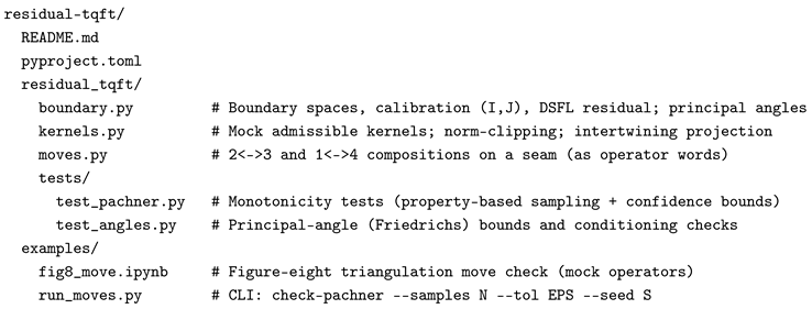
B. Core API (Pythonic Pseudocode with Enforcement)

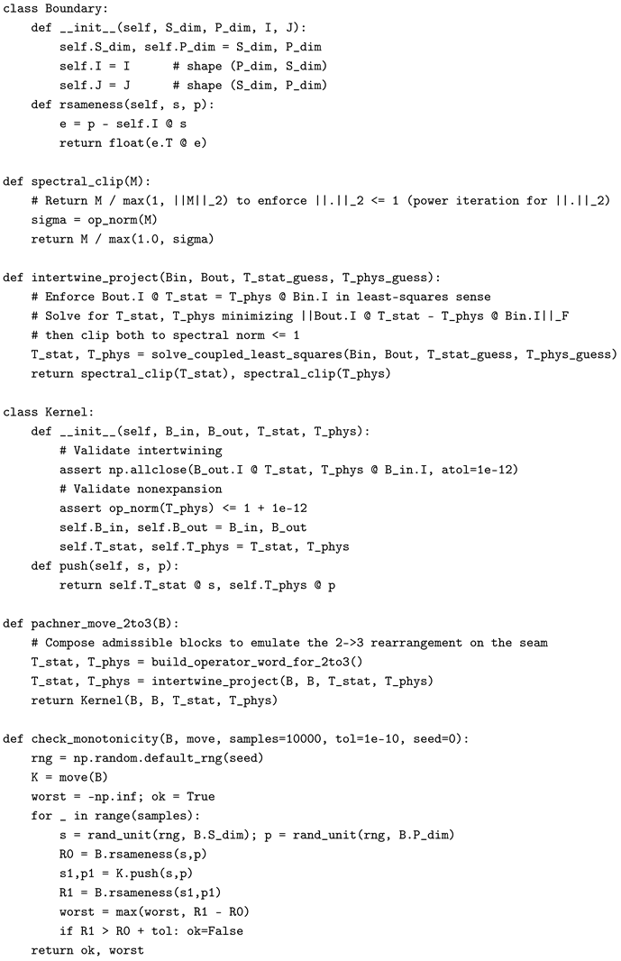
C. Acceptance Criterion and Statistical Confidence

A run passes if ok=True and the maximal defect ${\delta }_{max}=max(R_{\mathrm{after}}-R_{\mathrm{before}})\le {\epsilon }_{\mathrm{tol}}$ across N independent samples. To report confidence, model the indicator $Z_i=\mathbf{1}\{R_{1,i}>R_{0,i}+{\epsilon }_{\mathrm{tol}}\}$ ($i=1,\dots ,N$). If ${\sum }_i{Z}_i=0$, Hoeffding gives, for any $\eta \in (0,1)$,

$$\mathbb{P}\left(\mathbb{E}\left[Z_1\right]\ge \eta \right)\le e^{-2N{\eta }^2}.$$

Thus with $N={10}^4$ and $\eta ={10}^{-2}$, observing no violations certifies that the true violation rate is $<1\%$ with probability at least $1-e^{-200}\approx 1$; larger N pushes the bound lower. (If some violations occur, report $\widehat{p}={\displaystyle \frac{1}{N}}\sum Z_i$ with an exact binomial CI.)

Numerical stability notes. 

• Intertwining enforcement. Use intertwine_project once per move instance to project a guessed pair $(T_{\mathrm{stat}},T_{\mathrm{phys}})$ onto the affine subspace $\{(X,Y):B_{\mathrm{out}}.IX=Y{B}_{\mathrm{in}}.I\}$, then clip both by spectral_clip.
• Operator norm. Estimate $\parallel T_{\mathrm{phys}}{\parallel }_2$ via the power method with a stringent stopping tolerance (e.g. ${10}^{-12}$); add a safety factor in the assertion.
• Principal angles (optional). Provide principal_cosine(Pin,Pout) via SVD of $P_{\mathrm{in}}{P}_{\mathrm{out}}{|}_{\mathrm{ran}\left(P_{\mathrm{out}}\right)}$ to log the conditioning proxy $\gamma$.

D. What the harness proves in practice

Under exact admissibility, Theorem 5 guarantees $R_{\mathrm{after}}\le R_{\mathrm{before}}$ pointwise. Under discretization, the harness verifies the $(\epsilon ,\delta )$–admissible variant (Thm. 6) by construction—intertwining error $\epsilon$ and norm inflation $\delta$ are made as small as numerically attainable by projection and clipping, and any remaining slack is detected in the empirical certificate.

Remark 2 

(Referencing the kernel facts). The only nontrivial analytic inputs we used are (i) the unitarity of the edge operator in the modular–double Plancherel representation and (ii) the operator pentagon identity, both classical for the Faddeev quantum dilogarithm [3,4,6,7,27]. The operator–algebraic identity (9) is standard for orthogonal conditional expectations onto MASAs (see, e.g., Kadison–Ringrose).

6. Afterword

The results above isolate what is universal: once every local gluing step acts as an intertwining contraction in a single comparison Hilbert geometry, the DSFL residual (1) is a bona fide Lyapunov functional for cutting & gluing. In the Teichmüller state–integral class, this hypothesis is realized by two structural facts—unitarity of the edge operator and the pentagon identity—so no special–function asymptotics are needed. We conclude by making this universality precise, recording robustness and limits, and sketching scientific consequences.

6.1. Universality Principle and a Converse

Theorem 10 

(Universality of residual Lyapunov law). Let ${\mathsf{H}}_{\Sigma }$ be a fixed comparison Hilbert space and $({\mathcal{I}}_{\Sigma },J_{\Sigma }^{(+)})$ a calibration. Suppose every elementary gluing step along any seam Σ is implemented by a linear pair $(\tilde{\Phi },\Phi )$ satisfying the admissibility conditions (2). Then for any composite gluing pipeline $\mathsf{G}={\prod }_k({\tilde{\Phi }}_k,{\Phi }_k)$ and any boundary data $(s,p)$ one has the chain of inequalities

$$\mathcal{R}({\tilde{\Phi }}_n\dots {\tilde{\Phi }}_{1}s,{\Phi }_n\dots {\Phi }_{1}p)\le \dots \le \mathcal{R}({\tilde{\Phi }}_{1}s,{\Phi }_{1}p)\le \mathcal{R}(s,p),$$

i.e. $\mathcal{R}$ is Lyapunov along the pipeline, independent of triangulation choices.

Proof. 

Iterate the data–processing inequality (Theorem 1). No additional structure is used. □

Theorem 11 

(A converse: Lyapunov ⇒ admissibility). Let $(\tilde{\Psi },\Psi )$ be a bounded pair such that $\mathcal{R}(\tilde{\Psi }s,\Psi p)\le \mathcal{R}(s,p)$ forall$(s,p)$. Then necessarily:

• Ψ is nonexpansive on theresidual directions: $\parallel \Psi e\parallel \le \parallel e\parallel$ for all e;
• Intertwining holds: $\Psi {\mathcal{I}}_{\Sigma }={\mathcal{I}}_{{\Sigma }^{\prime }}\tilde{\Psi }$.

If, moreover, ${\mathcal{I}}_{\Sigma }$ has dense range and $J_{\Sigma }^{(+)}$ is the orthogonal projector dual to ${\mathcal{I}}_{\Sigma }$ ( $\mathcal{I}{J}^{(+)}={\mathrm{id}}_{\mathsf{P}}$, $J^{(+)}\mathcal{I}=P_{\mathsf{S}}$ ), then $\parallel \Psi \parallel \le 1$ on $\mathsf{H}$.

Proof. 

Setting $p=\mathcal{I}s+e$ gives $\mathcal{R}(\tilde{\Psi }s,\Psi p)={\parallel \Psi e\parallel }^2$ and $\mathcal{R}(s,p)={\parallel e\parallel }^2$, hence $\parallel \Psi e\parallel \le \parallel e\parallel$ for all e. Taking $e=0$ forces $\Psi \mathcal{I}s=\mathcal{I}\tilde{\Psi }s$ for all s, i.e. intertwining. If $\mathrm{ran}\mathcal{I}$ is dense, any $x\in \mathsf{H}$ is a limit of residual directions $e_n=p_n-\mathcal{I}{s}_n$, hence $\parallel \Psi x\parallel \le \parallel x\parallel$ by continuity. □

Remark 3 

(Equivalence class viewpoint). Theorems 10–11 show that the Lyapunov property isequivalentto admissibility, once the calibration is fixed. Thus the DSFL residual upgrades “axioms of sewing” to anif and only ifcriterion:gluing is stable precisely when it is an intertwining contraction in the comparison geometry.

6.2. Robustness, Limits, and Failure Modes

Small violations. 

Section 3 (Thm. 6) shows $(\epsilon ,\delta )$–admissible steps produce at most quadratic slack. Hence discretizations that enforce intertwining up to $\epsilon$ and clip spectral norms at $1+\delta$ inherit a controlled near–Lyapunov property.

Failure modes. 

If either condition in (2) fails badly, monotonicity can break:

• Nonintertwining. If $\Psi \mathcal{I}-\mathcal{I}\tilde{\Psi }$ has large operator norm, the residual can inflate by $O(\parallel \Psi \mathcal{I}-\mathcal{I}\tilde{\Psi }{\parallel }^2\parallel s{\parallel }^2)$ even when $\parallel \Psi \parallel \le 1$.
• Expansion. If $\parallel \Psi \parallel >1$, then directions e in the top singular subspace inflate the residual by ${\sigma }_{max}{(\Psi )}^2$.

Both effects are observable and certifiable by the verification harness (§Section 5).

6.5. Categorical Consequences and Anomaly Bookkeeping

Proposition 13 

(Residual naturality and anomaly line). Let ${\eta }_{\Sigma }:={\Pi }_{\mathrm{DSFL},\Sigma }\circ {\mathbb{Q}}_{\Sigma }$ be the comparison map from a reference modular functor $\mathcal{M}$ to the residual functor $\mathcal{R}$. For any bordism $M:\Sigma \to {\Sigma }^{\prime }$ implemented by admissible kernels, the naturality square commutes up to a central phase:

$${\eta }_{{\Sigma }^{\prime }}\circ \mathcal{M}\left(M\right)=e^{i\vartheta \left(M\right)}\mathcal{R}\left(M\right)\circ {\eta }_{\Sigma },\vartheta :\mathbf{Cob}\to \mathbb{R}/2\pi \mathbb{Z}.$$

The phases assemble into a flat line bundle (the anomaly line). All DSFL inequalities are phase–insensitive.

Proof. 

Intertwining gives strict commutation before projecting; the DSFL projector is idempotent and bounded; phases multiply both sides by a unit scalar. □

6.6. Algorithmic and Numerical Consequences

Certification by supermartingales. 

For randomized pipelines $({\tilde{\Phi }}_k,{\Phi }_k)$ with $\mathbb{E}[\parallel {\Phi }_k{\parallel }^2|{\mathcal{F}}_{k-1}]\le 1$, the residual sequence $E_k=\mathcal{R}({\tilde{\Phi }}_k\dots {\tilde{\Phi }}_{1}s,{\Phi }_k\dots {\Phi }_{1}p)$ is a supermartingale (Thm. 7). This yields:

• almost–sure convergence of $E_k$;
• tail bounds for empirical violation rates via Hoeffding/Bernstein, enabling reproducible pass/fail certificates;
• linear semi–log decay when the mean contraction is uniform ($\mathbb{E}\parallel {\Phi }_k{\parallel }^2\le {\rho }^2<1$).

Seam conditioning. 

Principal angles between polarizations bound through–seam operator norms by $\parallel P_{\mathrm{out}}K{P}_{\mathrm{in}}\parallel \le \gamma =cos{\theta }_F$ (Prop. 9), giving: (i) sharp two–sided uncertainty for residual splits; (ii) a conditioning number $\kappa \left({\theta }_F\right)={\displaystyle \frac{1+\gamma }{1-\gamma }}$ to guide chart choices in numerics.

6.9. Teichmüller Specialization: Why It Works “for Free”

In the Teichmüller class, admissibility is guaranteed “from the start”: [14,28,29,30]

• Unitarity. The edge operator $\mathsf{T}$ (built from ${\Phi }_b\left(\widehat{p}\right)$ and the metaplectic Gaussian) is unitary on the modular–double Plancherel space.
• Pentagon identity. The $2\leftrightarrow 3$ move holds as a strong operator identity (no approximation).
• Pointer compatibility. Orthogonal conditional expectations onto MASAs commute with unitary conjugations of those MASAs (change of polarization).

Therefore every elementary move is an exact intertwining isometry on ${\mathsf{H}}_{\Sigma }$, and all of the above consequences apply verbatim.

6.10. Outlook: Envelopes, Modularity, and Testable Conjectures

DSFL envelopes and resurgence. 

When a coercive DSFL identity is available for tails $\mathfrak{R}$ (e.g. along steepest–descent thimbles), Grönwall yields exponential envelopes $\parallel {\mathfrak{R}}_N\parallel \le C^{\prime }{e}^{-(\alpha -C)N}$ (Thm. 9). Because admissible gluing preserves the minimum coercivity margin, rates are glue–stable: ${\alpha }_{\mathrm{glue}}\ge {min}_i{\alpha }_i$.

Quantum modularity link (program). 

In state–integral models for hyperbolic 3–manifolds, the nearest Borel singularity is the smallest real part among relative Chern–Simons actions. It is therefore natural to conjecture (and verify case by case) that the DSFL envelope rate equals that real part, and that it is preserved under JSJ gluing. This identifies a concrete bridge from DSFL Lyapunov rates to quantum modularity exponents.

Practical takeaway. 

From the DSFL vantage point, topology is what survives the flow: admissibility collapses metric minutiae and forces residual monotonicity. This gives a unifying, verifiable stability layer for cutting & gluing pipelines, exact recursion, and categorical sewing—together with quantitative, phase–insensitive error bars and robust numerical certification.

Author’s Note. 

This paper develops a sector-neutral Lyapunov–residual framework—the Deterministic Statistical Feedback Law (DSFL)—aimed at recovering standard equilibrium relations as dynamical attractors under explicit hypothesis gates. The intention is not to replace established formalisms, but to clarify their restoration mechanisms by isolating a minimal quadratic residual and its propagation–gap structure.

Declaration of Generative AI and AI-Assisted Technologies in the Writing Process: During preparation of this manuscript, the author used ChatGPT (OpenAI) for limited technical and editorial assistance, specifically to: (i) refactor small Python utilities (e.g., plotting, data wrangling) and translate brief code snippets between R and Python; (ii) convert draft formulas and definitions into LaTeX; and (iii) suggest wording and layout improvements for tables, boxes, and section headings. All outputs were reviewed, edited, and independently validated by the author. The author is solely responsible for the scientific content, analysis, and presentation.

References

- Ponsot, B.; Teschner, J. Liouville bootstrap via harmonic analysis on a noncompact quantum group. arXiv 2000, arXiv:hep-th/9911110. [Google Scholar]
- Fock, V.; Goncharov, A. Cluster ensembles, quantization and the dilogarithm. Annales Scientifiques de l’École Normale Supérieure 2009, 42, 865–930. [Google Scholar] [CrossRef]
- Andersen, J.E.; Kashaev, R. A TQFT from quantum Teichmüller theory. Communications in Mathematical Physics 2014, 330, 887–934. [Google Scholar] [CrossRef]
- Baseilhac, S.; Benedetti, R. Analytic families of quantum hyperbolic invariants. Algebraic & Geometric Topology 2014, 14, 1983–2063. [Google Scholar]
- Pachner, U. P.L. homeomorphic manifolds are equivalent by elementary shellings. European Journal of Combinatorics 1991, 12, 129–145. [Google Scholar] [CrossRef]
- Faddeev, L.D.; Kashaev, R.M. Quantum Dilogarithm. Modern Physics Letters A 1994, 9, 427–434. [Google Scholar] [CrossRef]
- Faddeev, L.D. Discrete Heisenberg–Weyl group and modular group. Letters in Mathematical Physics 1995, 34, 249–254. [Google Scholar] [CrossRef]
- Tomiyama, J. On the Projection of Norm One in W*-Algebras. Proceedings of the Japan Academy 1957, 33, 608–612. [Google Scholar] [CrossRef]
- Takesaki, M. Theory of Operator Algebras I; Springer, 2003.
- Fock, V.V.; Chekhov, L.O. Quantum Teichmüller space. Theoretical and Mathematical Physics 1999, 120, 1245–1259. [Google Scholar] [CrossRef]
- Matveev, S.V. Algorithmic Topology and Classification of 3-Manifolds; Vol. 9, Algorithms and Computation in Mathematics, Springer, 2007.
- Kadison, R.V. A generalized Schwarz inequality and algebraic invariants for operator algebras. Annals of Mathematics 1952, 56, 494–503. [Google Scholar] [CrossRef]
- Atiyah, M.F. Topological quantum field theories. Publications Mathématiques de l’IHÉS 1988, 68, 175–186. [Google Scholar] [CrossRef]
- Dimofte, T.; Gaiotto, D.; Gukov, S. 3-Manifolds and 3d Indices. Advances in Theoretical and Mathematical Physics 2013, 17, 975–1076. [Google Scholar] [CrossRef]
- Kadison, R.V.; Ringrose, J.R. Fundamentals of the Theory of Operator Algebras. Vol. I: Elementary Theory; Vol. 15, Graduate Studies in Mathematics, American Mathematical Society: Providence, RI, 1997.
- Kadison, R.V.; Ringrose, J.R. Fundamentals of the Theory of Operator Algebras. Vol. II: Advanced Theory; Vol. 16, Graduate Studies in Mathematics, American Mathematical Society: Providence, RI, 1997.
- Bhatia, R. Matrix Analysis; Vol. 169, Graduate Texts in Mathematics, Springer: New York, 1997. [CrossRef]
- Halmos, P.R. Two Subspaces. Transactions of the American Mathematical Society 1969, 144, 381–389. [Google Scholar] [CrossRef]
- Nielsen, M.A.; Chuang, I.L. Quantum Computation and Quantum Information, 10th anniversary edition ed.; Cambridge University Press: Cambridge, UK, 2010. [Google Scholar]
- Petz, D. Monotonicity of Quantum Relative Entropy Revisited. Reviews in Mathematical Physics 2003, 15, 79–91. [Google Scholar] [CrossRef]
- Davis, C.; Kahan, W.M. The Rotation of Eigenvectors by a Perturbation. SIAM Journal on Numerical Analysis 1970, 7, 1–46. [Google Scholar] [CrossRef]
- Banach, S. Sur les opérations dans les ensembles abstraits et leur application aux équations intégrales. Fundamenta Mathematicae 1922, 3, 133–181. [Google Scholar] [CrossRef]
- Doob, J.L. Stochastic Processes; Wiley, 1953.
- Hoeffding, W. Probability inequalities for sums of bounded random variables. Journal of the American Statistical Association 1963, 58, 13–30. [Google Scholar] [CrossRef]
- Björck, Å.; Golub, G.H. Numerical Methods for Computing Angles between Linear Subspaces. Mathematics of Computation 1973, 27, 579–594. [Google Scholar] [CrossRef]
- Kashaev, R.M. Quantization of Teichmüller spaces and the quantum dilogarithm. Letters in Mathematical Physics 1998, 43, 105–115. [Google Scholar] [CrossRef]
- Dimofte, T.; Gaiotto, D.; Gukov, S. Gauge theories labelled by three-manifolds. Communications in Mathematical Physics 2011, 325, 367–419. [Google Scholar] [CrossRef]
- Kashaev, R.M. The Hyperbolic Volume of Knots from the Quantum Dilogarithm. Letters in Mathematical Physics 1997, 39, 269–275. [Google Scholar] [CrossRef]
- Andersen, J.E.; Kashaev, R. A TQFT from Quantum Teichmüller Theory. Communications in Mathematical Physics 2014, 330, 887–934. [Google Scholar] [CrossRef]
- Andersen, J.; Kashaev, R. A TQFT from quantum Teichmüller theory. Communications in Mathematical Physics 2014, 330, 887–934. [Google Scholar] [CrossRef]