Submitted:
27 November 2025
Posted:
28 November 2025
Read the latest preprint version here
Abstract
In this article the relationships are revealed between the views on neutrinos as they show up in various approaches of study. Among these are (a) Fermi’s theory on beta decay, (b) the classical view on the decay of the pion into a muon and a muon neutrino, (c) instrumental attempts for direct measurements of the neutrino’s rest mass like in the KATRIN project, (d) the studies in modern neutrino observatories on the phenomenon of neutrino oscillation and (e) the view on neutrinos in the Structural Model of particle physics. A non-classical kinematic analysis on lab frame decay processes shows that the effective masses of the three neutrinos are the same, although in this respect the comparison with the present data in the PMNS theory is not fully conclusive. Adopting the hypothesis that neutrinos fly at the lab frame speed of pions in free flight, their rest masses have to be set at 182.5 meV/c2.
Keywords:
neutrino flavours
; mass eigenstates
; PMNS matrix
; beta decay
; KATRIN
1. Introduction
In a preceding article [1] on the subject, a physical model has been shown for the relationship between a pion, a muon and a muon neutrino. This model allows to give a mathematical description for the wave equation of the muon neutrino in energetic state. The wave equation has been described in terms of a two-body quantum mechanical oscillator model that reveals three quantum states for the vibration energy in the centre-of-mass. An attempt has been made to relate the energetic quantum states of the neutrino flavours with the three mass eigenstates that show up in the PMNS theory that presently is considered as the canonical theory of neutrinos [2]. This attempt failed and no decisive relationship has been found between the quantum states of the neutrino flavours and the mass eigenstates of the PMNS theory.
The model, though, allows to incorporate the tauon and the tauon neutrino in the model. These two particles are the products of a decay mode of the charmed meson ( or). The incorporation of the tauon/neutrino twin is possible because of the recognition, shown in the Structural Model, that the tauon is an excited state of the muon and that the charmed meson is an excited state of the pion. This recognition has been underpinned by the calculated and empirically proved mass relationships between the particles. Unfortunately, whereas the tauon/neutrino twin could be physically related with the muon/neutrino twin, the relationship between the electron/neutrino twin didn’t have a firm theoretical relationship and has been simply adopted because of symmetry reasons. Recently though, the author of this article has calculated the mass of the electron from first principles of the Structural Model, thereby showing the mass relationship between the muon and the electron by theory. It means that one of the two issues left open has been solved [4]. The other issue, namely the problem how to give a quantitative explanation for the contents of the PMNS matrix, is still open.
What I wish to do in this article is showing the mass relationships of the neutrinos in flavour states and to demonstrate how these mass relationships relate with the mass eigenstates in the PMNS matrix. Figure 1 shows the relationship between the three lepton twins as come forward from the structural view on particle physics [3]. It gives a structural interpretation (a) for the decay of a pion into a muon and a muon neutrino , (b) for the decay of a muon into two neutrinos and an electron and (c) for the excitation of a pion into a charmed meson. This interpretation is based upon the awareness that the W boson has to be regarded as the relativistic state of the rest mass of the pion. The justification of this awareness has in extenso been justified in [3]. It means that the decay of the pion state into the electron state is modeled as the muon/neutrino frame representation of the pion, similarly as the excitation of the pion state to the charmed meson state.
The two-body quantum mechanical models for the mesons, the charged leptons and the neutrinos are intimately related, but slightly different [1]. The three quantum states of the neutrinos are represented in the figure by dashed lines at the top of the figure. We shall use this model to calculate the rest masses of the neutrinos in flavour state. The virtue of this model is the clear distinction between the masses of the neutrinos in flavour state on the one hand and the quantum statesof the neutrinos on the other hand. The latter are usually denoted as mass eigenstates. This is a source for confusion. In fact, the quantum state model of the three neutrinos is the same in the sense of relative quantities, but might be different in the sense of absolute quantities.
The picture to take into mind is the advent of high energetic cosmic pions entering in the atmosphere. The pions convert their energy into a muons and muon neutrinos, or, alternatively, into electrons and electron (anti)neutrinos. Eventually, it is the internal energy of the pion that gets a different format. The pion’s internal energy is manifested as a W boson. This allows to consider the W boson as the relativistic state of the pion’s rest mass. We wish to consider the decay processes involved as the disintegration of the energy of the W boson into the state of observable fermions.
Let us start with the decay of a pion into the muon and the muon neutrino. Denoting the momenta of, respectively, the pion, the muon, and the neutrino, as and and their Einsteinean energies as and , we have, because of conservation of momentum
and, because of conservation of energy,
Usually the system is considered in the rest frame of the pion, which in the Structural Model of particle physics is an adequate representation for the lab frame. Furthermore, we wish to express the velocities of the particles in terms with their difference with the speed of light in vacuum. Hence, generally as . This will enable to conveniently exploit the knowledge that the W boson can be regarded as the pion’s rest mass in relativistic state. The rest masses of the particle will be written as, respectively, and , and the associated energies of that state as and .
2. The Classical Model
In the classical description of the pion’s decay process the momentum relationship (1) is reduced to [5],
This can be written as,
Assuming that the neutrino flies at light speed, the energy relationship can be written as,
Multiplying (4) with c and subtraction, gives
Subsequent evaluation gives,
In the classical approach, the decay process is considered in the rest frame of the pion. In this rest frame . Hence,
From this result, the magnitudes of the quantities summarized in Table 1 can be easily assessed.
These results are well-known common analyses that take the rest frame of the pion as reference. In this frame the muon neutrino flies away with an energy to the amount of 29.79 MeV.
2.1. The Passenger Model
Unfortunately, the energy value is not enough to estimate the rest mass of the muon neutrino in its flavour state. A reasonable hypothesis would be that the neutrino flies away at the same speed that the pion had before it came to rest, because “when a car stops suddenly, passengers are thrown forward due to inertia. Inertia is the tendency of an object to resist changes in its state of motion. When the car stops, the passengers’ bodies continue moving forward at the car’s previous speed". Hence, if this pion speed would be known, the neutrino speed would be known from the passenger’s model. The Structural Model of particle physics gives a clue here, because in that model the energy of the W boson is the rest mass of the pion in relativistic state. Because the W boson is the rest mass of the pion flying at high speed, we have in this condition for ,
Hence, in this concept the neutrino with its energy of 29.79 MeV flies away at a speed . Therefore, the rest mass of the neutrino would show up as , in which . The resulting magnitude is 51.7 keV/. The result of this passenger model fits with reported results from experimental set-ups for direct measurement of the muon neutrino [6]. The caveat, though, is the violation of the initial assumption that the neutrino flies at light speed and is mass less. Another issue is the question how to address the electron neutrino and the tauon neutrino problem. The just given estimate for the muon neutrino is far beyond the scale of the upper limit of 0.8 eV reported from the KATRIN experiment [7], which on its turn is far beyond the scale of 18 – 50 meV from model based predictions from studies on the oscillating phenomenon of extremely high energetic cosmological neutrinos [8].
3. The Non-Classical Model
In this paragraph another route is followed. Rather than considering the pion in its rest frame, the pion will be analyzed in its relativistic state. To do so we rewrite the two basic equations now as
Rewriting (10b)
Multiplying (11a) by , and subsequent subtraction gives,
Replacing the variable by the variable , such that,
allows to rewrite (12) as,
and, equivalently,
Eqs. (14-15) allow us to calculate if would be known. Subsequently the neutrino energy can be found from (10b). Generically as,
We wish to proceed by considering the implications of this analysis for three decay modes that are responsible for the production of neutrinos. These modes are formally denoted as,
3.1. The Muon Neutrino
The application of (16) on the pion decay into muon and a muon neutrino allows to calculate the rest mass of the muon neutrino as a function of , as shown in Figure 2. At the rest mass is 58.9 keV/. This corresponds with the result obtained in the classical approach with the passenger model.
The result, though, requires a careful interpretation. The numerical calculation shows that the energy of the muon neutrino at the speed of the pion prior to decay can be traced back to of the energy of the boson. The other is transferred to the muon. No more, no less. Actually, though, the spread of the energy of the pion under decay is a statistical process that is subject to Fermi’s law of beta radiation. The implication of this consideration will be clear if we apply the same theory to the decay of a pion into an electron and an electron (anti)neutrino.
3.2. The Electron Neutrino
Let us proceed by considering the decay of the pion into an electron and an electron (anti)neutrino. A straightforward application of the analysis presented in the previous paragraph reveals that, under decay, the (anti-)neutrino takes almost all energy from the pion to an amount of , thereby leaving only for the electron. In that view, the rest mass of the neutrino, flying at the same speed of the pion prior to decay, would amount to 241 keV/. And this is a result far beyond the scale obtained from direct measurements on beta radiation, such as, for example, shown in the KATRIN project.
The approach in the KATRIN project is a direct application of Fermi’s beta radiation theory. It is a large-scale physics experiment in Germany, designed to measure the mass of the electron neutrino with unprecedented sensitivity. It studies the energy spectrum of electrons emitted in beta decay from tritium to helium-3 as formalized by
The atomic number difference between tritium and helium-3 in terms of energy is only 18.6 keV, which known to a precision of about 2 eV. Regardless of neutrino mass, the kinetic energy of the radiated electrons cannot exceed the limit of 18.6 keV + 0.2 eV. This kinetic energy is measured by applying a retarding electric potential to the radiated electrons. Electrons can only come from the endpoint of its energy spectrum. If the neutrino has some mass, this endpoint is slightly below the limit of 18.6 keV + 0.2 eV. Hence, the difference between the endpoint and the limit must be due to the rest mass of the neutrino. Fixing the endpoint of the electron spectrum requires a statistical analysis of electron counts over a narrow retarding potential window near the limit of 18.6 keV + 0.2 eV. The heart of the experimental equipment is a 70-meter-long spectrometer, one of the largest ultra-high vacuum vessels ever built. By achieving sub-eV precision, KATRIN aims to set the most stringent direct upper limit on neutrino mass. At present, this upper limit is set at 0.8 eV. Our theoretical analysis in the preceding, though, predicts a result far beyond this scale. How to explain the discrepancy?
3.3. Fermi’s Theory
In Fermi’s theory beta radiation is a process subject to the limitations of the density of states formalized by the Fermi-Dirac statistics [9,10]. Fermions, such as, for example, charged leptons (electron, muon, tauon) and neutral leptons (neutrinos) generated in a decay process, can only fill a state of energy if this state is freely available and not already filled by another fermion in the same state of spin. This implies that the decay process of the type described in the previous paragraphs is not a deterministic one, but a statistical one instead. A close inspection of the analysis presented so far reveals that the only parameter that can be made accountable for statistical behaviour is the scattering angle in (1). For convenience we have adopted for analysis. Quite probably, this condition reveals just an extreme result for the statistical distribution of the possible energies that a neutrino may adopt under decay. This view suggests that another extreme could show up for . A slight modification of eqs. (10 – 16) allows to inspect the consequences of this consideration. Rewriting and modifying (10) gives,
Multiplying (19) by c, and subsequent addition gives,
Replacing the variable by the variable , such that,
allows to rewrite (20) as,
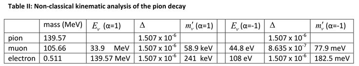
Note that the only difference between the collinear case and the anti-linear case is the sign difference between (13) and (21). The result of the rest mass calculation, though, is dramatically different. The results of the calculation for and , for the pion decay into, respectively, a muon and an electron, are summarized in Table 2. It shows that rest mass of the electron (anti)neutrino, if, taking the rest frame of the pion as the lab frame, amounts to 182.5 meV/ only if would fly at the speed of the pion prior to decay. As a function of it behaves as shown in Figure 3.
This result is of an order of magnitude that is expected as a future result from the KATRIN experiment .
Applying the same analysis to the decay of the pion to the muon and the muon neutrino reveals that rest mass of the muon neutrino is less and amounts to 77.9 meV/ only. The large relative difference with the rest mass of the neutrino gives some doubt whether the comparison has been made on equal footing.
The only thing that we know that if the speed of the electron neutrino is equal to the speed of the pion prior to decay, its rest mass amounts to 182.5 meV/. But there is no compelling reason why this would be the case. The same holds for the muon neutrino. There is no compelling reason why the muon neutrino would fly at that speed either. It might well be that the two neutrinos under decay from the pion move at different speeds. It is quite probable that the muon neutrino speed is different, because the decay from the pion state to the muon state is a smaller step in energy than the decay of the pion to the electron state. This is clearly demonstrated in the collinear case . As we have seen before, in that case we have from (14), taking into consideration that
As known from (9),
which implies that . Hence
Inserting this result in (10a) gives,
Because , the muon neutrino flies at a significantly lower speed than the electron neutrino. The two neutrinos can now be brought on equal footing by a correction factor obtained from (26) as,
What does it say? It says that the effective mass of a muon neutrino under appropriate scaling from an electron neutrino, would amount to 77.9/0.4269 = 182.5 meV. It brings the effective mass of the muon neutrino at the same level as the effective mass of the electron neutrino. Because we are not sure if the speed of the pion prior to decay is the actual speed of the electron neutrino, the concept effective mass replaces the concept rest mass.
3.4. The Tauon Neutrino
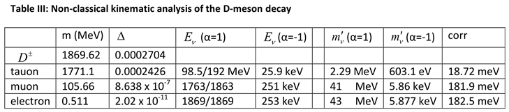
The comparison of properties between a muon neutrino and an electron neutrino appeared being possible because of the existence of a physical process in which both particles have a common origin. The particles are products in two decay modes from the archetype meson (pion). To include the tauon neutrino (the third flavour) in this comparison we would need a common decay process for all three flavours. Fortunately, the meson has three independent decay modes for the three flavours. Applying the same analysis as for the pion decay before, results are shown as summarized in Table 3.
The last three columns are worthwhile to be discussed. The difference in neutrino mass between and needs no further discussion. Because the neutrinos are generated from the meson, and because the meson is (in the Structural Model) a pion in a higher state of energy, the generated neutrinos are in a higher state of energy as well. Note that the calculated mass values of the neutrino are valid on neutrino speed . But the value for the meson is quite different from the value of the pion. The neutrinos generated from the meson decay move at a much lower speed than the neutrinos generated from the pion decay. A proper comparison should be made on equal footing. This requires a comparison on equal speed. Hence, whereas the electron neutrino shows up with a mass of 5.87 keV, it shows up at at a much lower value. The mass scaling factor can be readily established as,
As shown in Table 3, it brings the rest mass of the electron neutrino at the very same level as with the pion decay. It proves the correctness of the scaling factor.
The unscaled tauon neutrino shows a mass 603.1 eV at . Applying the mass scaling factor gives an effective mass for the neutrino of only 18.72 meV. However, as discussed before, this not the only scaling factor to be taken into account. Similarly, ass discussed before, a momentum correction is required to bring the tauon neutrino on equal footing with the electron neutrino. Denoting the scaling factor for the tauon neutrino with respect to the electron neutrino as , we have
It means that the tauon neutrino would show up at the level of the electron neutrino with an effective mass of 18.72/0.102614 = 182.5 meV.
The values in Table 3 for the muon neutrino need a correction as well. They are underestimated as well because of the momentum scaling factor difference between the electron neutrino and the muon neutrino. It needs a correction factor to the amount of,
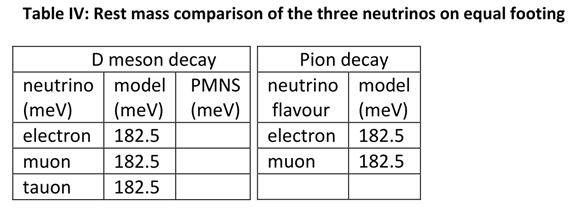
This brings the corrected effective mass for the muon neutrino at 182.5 meV. Table 4 gives the summary for the three neutrino flavours compared on equal footing. It shows a third column (PMNS), which will be discussed in paragraph 4.
It is worthwhile to note, but may be superfluous, that applying the same analysis on the decay modes of the gives the same result. It is just an additional confirmation of the viability of this kinematic approach.
Important:
It is quite remarkable, and, taking into account the very different decay schemes, even more or less astonishing, that the calculated effective masses for the three neutrinos are the same to a high amount of precision. It is an unexpected result that implies that the three neutrinos are basically the same, although being manifest at different propagation speeds.
3.5. The Correspondences and the Differences Between the Three Neutrino Flavours
We have seen so far that the neutrino in pion decay shows up in two modalities. The muon modality seems to have a higher speed and a lower rest mass than the electron modality. If the rest masses would be different indeed, the muon neutrino and the electron neutrino would be different particles. Like we have seen, corrected for speed, the modalities show the same rest mass. The paradox is solved by considering the two modalities as flavours of the same particle denying the rest mass as a useful attribute and replacing it by effective mass. Knowing from experimental evidence that the neutrino flavours are uniquely bound to their parental charge lepton, there must be a difference, though. In the Structural Model of particle physics [3] it has been shown that neutrinos have three different quantum states. The unique bond between the parental leptons and the neutrinos can be explained by adopting the view that the flavours are in a difference mixture of these quantum states. This conclusion holds for the tauon neutrino as well.
It leaves the question if for neutrinos, next to rest mass, speed is a meaningful attribute either. In fact, the neutrinos are as indistinguishable in speed as they are in effective mass. What is useful though, if not required, is defining a reference level. The reference level adopted in our analysis, is a hypothetical speed level for the electron neutrino. This speed is set equal to the speed of the pion in free flight, just before decay. This speed can be calculated from the view shown in the Structural Model that the W boson can be seen as a pion in relativistic state. It may represent actual speed, for instance in the KATRIN project, or not. The lowest state of energy that a neutrino may have is the lowest state of energy that an electron neutrino has under pion decay. In that state the neutrino has an effective mass of 182.5 meV.
4. Comparison with the (Empirical) PMNS Model
Observations on solar neutrinos and cosmic neutrinos in suitably designed and built detectors have revealed that neutrinos may change their flavour and will show up as an oscillating mixture. These observations have led to a neutrino model that decomposes each of the three flavours into a characteristic mixture of three mass eigenstates. This model has been developed over the years into a well established theory (PMNS), pioneered by Ziro Maki, Masami Nakagawa and Shoichi Sakata [2], based upon pioneering work of Bruno Pontecorvo in 1957 [11]. That work is a ground breaking concept that does not fit in the canonical Standard Model of particle physics. It is seen as an element in “new physics”. The adoption of a paradigm shift from the Standard Model was necessary to explain the experimentally found phenomenon of flavour oscillations in solar and cosmic neutrinos. The view on neutrinos that are produced in the lab frame decay processes that has been developed in the previous chapter, nicely fits with this view. In that respect, the Structural Model of particle physics, on which this view has been developed, would be “new physics” as well, although the author prefers to see it as “common sense physics”.
The PMNS theory recognizes three flavor components, i.e., an electron neutrino, a muon neutrino and a tauon neutrino, that are built up as a mixture of mass eigenstates such that
in which is a 3 x 3 unitary matrix, known as the canonical PMNS matrix. This matrix is unitary and its coefficients are potentially complex. The coefficients of this matrix are determined from an interpretation of observations in the modern impressive huge underground neutrino detectors. It is basically a curve fitting procedure on measurement results. It is subject to a continuous update over the years.
To calculate effective masses from the canonical matrix, the matrix is modified to a matrix in which the coefficients are replaced by their magnitude or by the square of these . The most actual update (NuFIT 5.2) of the “magnitude” and “absolute squared” PMNS matrix gives [13],
and, squared
These matrices are no longer unitary. The squared absolute PMNS matrix shows the interesting feature that the coefficients in the rows as well as in the columns sum up to 1. It reflects the probability semantics of this matrix. In fact, under proper relabeling of, respectively, the mass eigenstates and the flavour states, the semantics are conserved under interchange of the columns and interchange of the rows. This property, however, is no guarantee that the underlying canonical PMNS matrix is unitary. The reverse, though, is true. The underlying unitary matrix might have complex coefficients. These coefficients can be traced back to three canonical mixing angles and a skewing angle . The present NuFIT5.2 data are [13],
While the accuracy of the mixing angles is well established, it is not the case for the phase angle parameter, parameter, which may assume any value between and [12].
Let us discuss this empirical result with the achievements presented in the previous section in mind. In the PMNS theory, the 3 x 3 unitary matrix is built up by three unitary rotation matrices and , such that ,
From a mathematical point of view there is no reason why the resulting overall matrix should be composed by real coefficients only. Unitarity can be preserved if, next to the rotation angles, one or more phase angles are added, for instance by an additional matrix
Let us omit the matrix for further discussion later.
To calculate effective masses from the canonical matrix, the matrix is modified to a matrix in which the coefficients are replaced by their magnitude or by the square of these , such that
Let us write the general format of the as
From the unitarity properties of the composing rotation matrices it is found that the algebraic sum of the coefficients in any of the three rows and columns of this matrix is equal to unity. If we would like to trace back the three mixing angles, we have to solve the equation set,
We may proceed by taking into account the result of the kinematic analysis of the lab frame decay processes,
and by invoking the empirical result obtained from the oscillation observations,
Using (39-41) the equation set (37) evolves to,
in which We have three equations with four unknown variables. These are the mixing angles and the mass parameter . Hence, the set is ill-conditioned.
When solar neutrinos are born, they consist of electron neutrinos that in free flight are subject to a change of their profile as a result of the unitary mixing process with muon neutrinos and to a negligible amount with tauon neutrinos. In that respect the solar neutrinos are different from the far more energetic cosmic neutrinos. It means that for solar neutrinos the U matrix can be approximated by a 2 x 2 one, instead of a 3 x 3 one. Hence, for solar neutrinos we have, instead of (43-45),
Unlike the (43-45) set, the set (46-47) is well conditioned. It contains a single unknown mixing angle and a unknown mass parameter . The solution of this set is,
If we now assume that the neutrino mixing angles are energy independent parameters, we may use the result of this mixing angle as an additional condition on the set (43-45) to make it well conditioned. Solving this equation set results in a slightly different matrix, which under interchange of the columns and interchange of the rows, closely resembles the NUFIT5.2 matrix shown before. The result is,
Retrieving the mixing angles from this matrix, we find,
This result shows a fair fit with the NuFIT5.2 values shown in (33). It has to be noted though that the value up-front parameter has been modified as a consequence of the interchange of columns and rows in the matrix. The interchange, though, has no physical impact, in spite of this modification. Proof for this can be found in literature [14]. The three mass eigenstates are, respectively,
while the three flavour masses are all the same (182.5 meV).
5. Discussion
The kinematic analysis of the decay processes discussed in this article has revealed some novel results. The most important one is the proof that the effective masses of the three neutrino flavours are equal. Although some arguments have been presented that these values amount to 182.5 meV, the true proof for its actual value is still missing, because the PMNS matrix as discussed in the previous paragraph is invariant for it. The PMNS matrix is invariant as well for the (Charge Parity) matrix part . It is instructive to emphasize that this matrix part has been introduced to fill out a mathematical degree of freedom, thereby maintaining Pontecorvo’s hypothesis that neutrinos could show violation. Evidence for this is still missing [15]. Although in this article a comprehensible physical explanation is given for the structure of the PMNS matrix, a physical explanation for the numerical values of the two squared mass differences of the mass eigenstates is still missing. It remains a subject for further research. What has to be researched further as well is giving an explanation for the slight difference between the NuFIT5.2 matrix as derived from empirical evidence on solar neutrinos and cosmic neutrinos and the PMNS matrix found from the analytical result that the effective masses of neutrinos that show up in lab frame decay processes are equal to a high amount of precision. The NuFIT5.2 matrix doesn’t seem fully compatible with that phenomenon.
6. Conclusions
1.The result of the kinematic analysis of four decay processes from mesons to leptons as presented in this article corresponds excellently with the empirical results obtained from the measurements in the modern neutrino observatoria that are based on the heuristic PMNS theory.
2. The kinematic analysis proves that the effective masses of the three neutrinos are the same. The numerical NuFIT5.2 fit on measurement results, though, shows a slight difference between the effective masses. Further research is required to explain the reason for the slight difference. It does not seem large enough to conclude that the nuFIT5.2 data are adequate to proof or to disprove the result of the kinematic analysis that the effective masses are the same.
3. Adopting the hypothesis that neutrinos fly at the lab frame speed of pions in free flight, their rest masses have to be set at 182.5 meV/.
References
- Roza, E. 2025: On the mass states and flavor states of neutrinos, www.preprints.org. [CrossRef]
- Maki, Z.; Nakagawa, M.; Sakata, S. 1962: Remarks on the unified model of elementary particles, Progr. of TheorPhysics. 28 (5): 870 (1962).
- Roza, E. 2025: Introduction to the Structural Model of particle physics, Kindle Books ISBN 978-90-90401-461.
- Roza, E. 2025: An old problem solved: Why the mass of the electron is 0.511 MeV/c2, www.preprints.org. [CrossRef]
- Energetics of pion decayhttp:hyperphysics.phy-astr.gsu.edu/hbase/Particles/piondec.html.
- Assamagan K. et al. 1996: Upper limit of the muon-neutrino mass and charged-pion mass from momentum analysis of a surface muon beam, Physical Review D: Particles and fields, 53 (11).
- Aker et al. (KATRIN Collaboration) 2022:Direct neutrino-mass measurement with sub-electronvolt sensitivity, Nature Physics 18, 160.
- Navas S. et al. (Particle Data Group), Phys.Rev. D110, 030001 (2024) and (2025) update.
- Ferni, E. 1934: Versuch einer Theorie der Beta Strahlen, Zeitschrift fur Physik 88, 161.
- Griffiths, D: Introduction to Particle Physics, John Wiley and Sons, p.309.
- Pontecorvo, B. 1957: Mesonium and anti-mesonium, Sov. Phys. JETFP 51 (6) (1957).
- Esteban I. et al. 2020: The fate of hints: updated global analysis of three-flavor neutrino oscillations, JHEP 09 178,.
- www.nu-fit.org.
- Junxing Pan, Jin Sun, Xiao-Gang He (2020): Neutrino Mixing, Which Convention? Int.J.Mod.Phys. A34 1950235, arXiv:1910.06688.
- Giunti C. and Kim Chung (2007): Fundamentals of Neutrino Physics and Astrophysics, ch. 12.3-12.5, Oxford Univ.
Figure 1.
The decay of the pion to the electron and the excitation of pion to the charmed meson (= decay of the charmed meson to the pion)
Figure 1.
The decay of the pion to the electron and the excitation of pion to the charmed meson (= decay of the charmed meson to the pion)
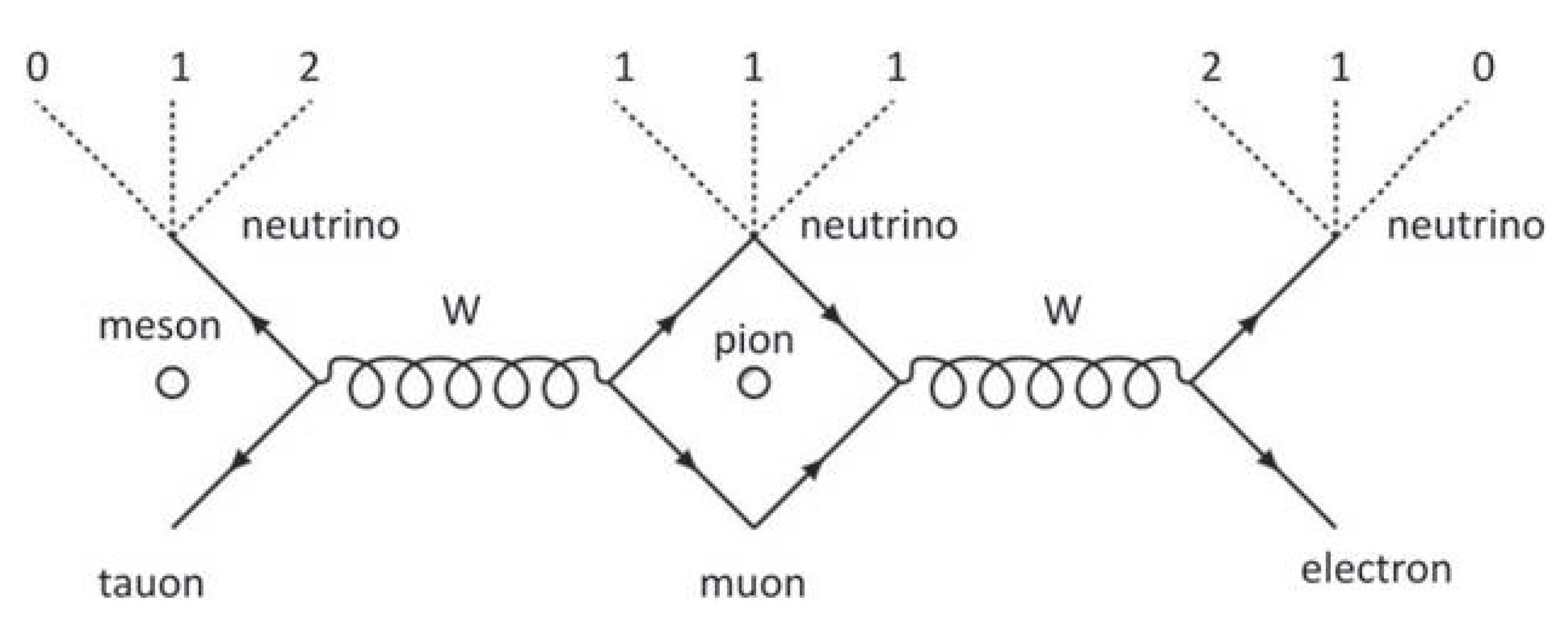
Figure 2.
The result of the kinematic analysis of the pion decay into a muon and a muon neutrino. It shows the rest mass of the muon neutrino as a function of its velocity when it flies away collinearly with the pion
Figure 2.
The result of the kinematic analysis of the pion decay into a muon and a muon neutrino. It shows the rest mass of the muon neutrino as a function of its velocity when it flies away collinearly with the pion
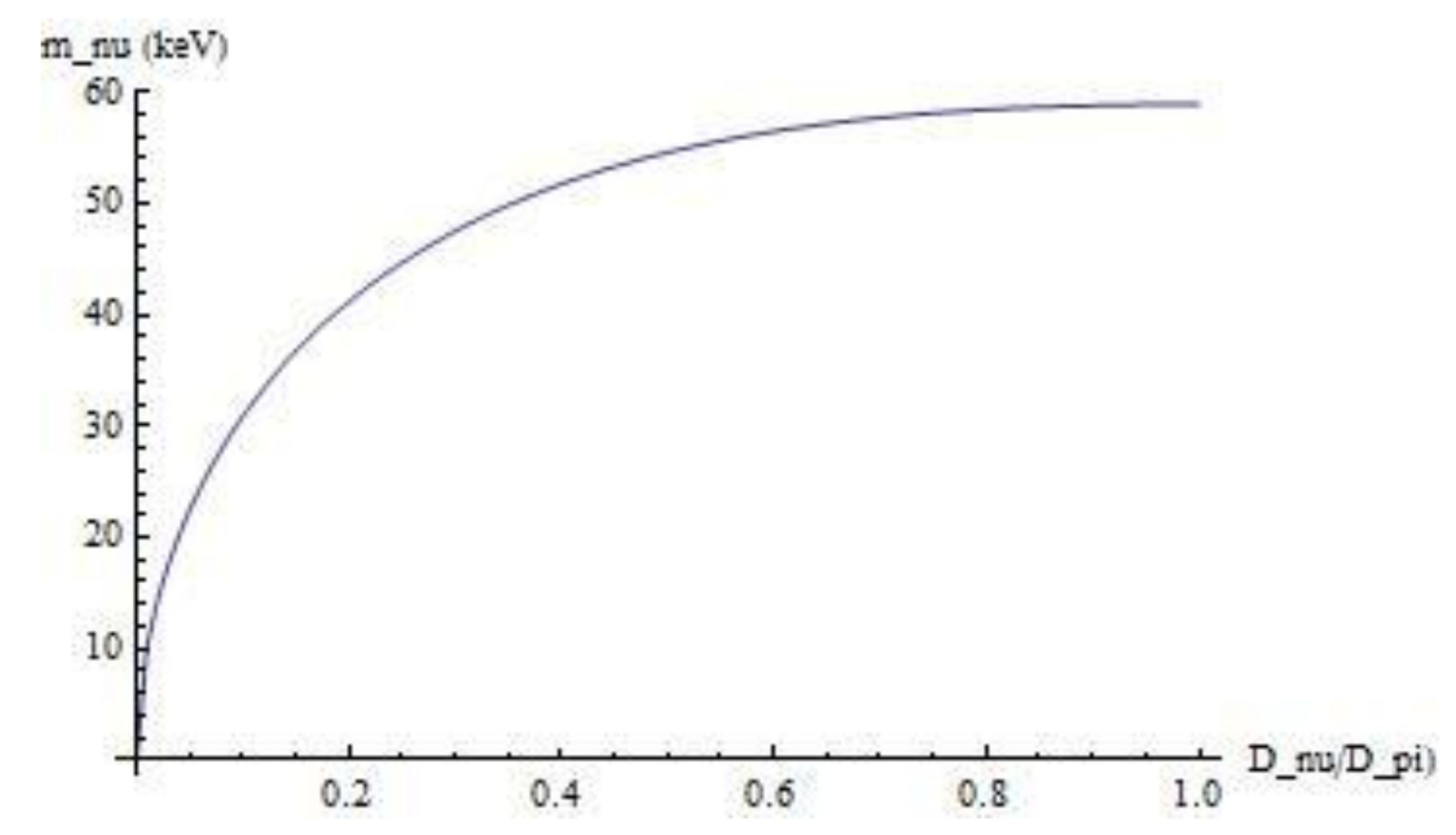
Figure 3.
The rest mass of the electron neutrino as a function of its velocity when it flies away ant-linearly from the decaying pion.
Figure 3.
The rest mass of the electron neutrino as a function of its velocity when it flies away ant-linearly from the decaying pion.
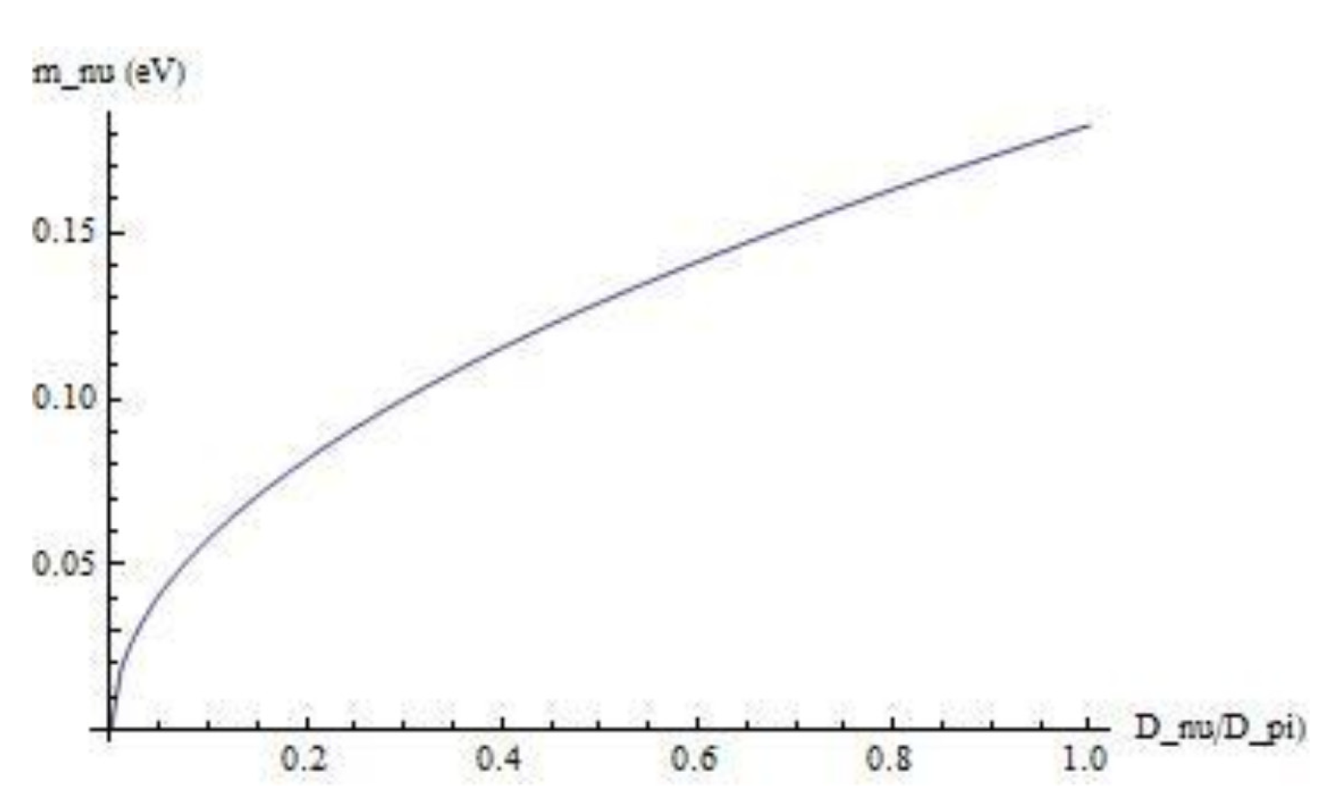

Table 1.
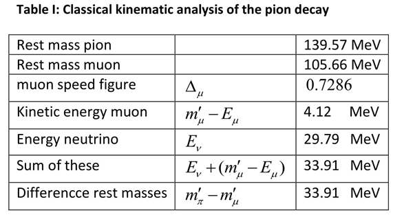 |
Table 2.
 |
( = cos )
Table 3.
 |
( = cos )
Table 4.
 |
Disclaimer/Publisher’s Note: The statements, opinions and data contained in all publications are solely those of the individual author(s) and contributor(s) and not of MDPI and/or the editor(s). MDPI and/or the editor(s) disclaim responsibility for any injury to people or property resulting from any ideas, methods, instructions or products referred to in the content. |
© 2025 by the authors. Licensee MDPI, Basel, Switzerland. This article is an open access article distributed under the terms and conditions of the Creative Commons Attribution (CC BY) license (http://creativecommons.org/licenses/by/4.0/).
Copyright: This open access article is published under a Creative Commons CC BY 4.0 license, which permit the free download, distribution, and reuse, provided that the author and preprint are cited in any reuse.


