Submitted:
20 October 2025
Posted:
21 October 2025
You are already at the latest version
Abstract
This paper introduces a Risk-Adjusted Stability Index (RASI) that summarizes banking-system stability from a single state variable, the banking Z-score, by integrating its level, trend, and risk dimensions. The index multiplies the mean Z-score by a concave, non-negative transformation of the estimated trend (geometric-mean log growth, with a Theil-Sen estimator in log space as a robustness alternative) and divides by dispersion in Z-score levels (baseline: population standard deviation; robustness: median absolute deviation × 1.4826, interquartile range / 1.349, and downside semi-deviation). Annual data for 2007-2021 are used with an inclusion rule of at least eight valid observations per country; an extended 2000-2021 window supports replication. Uncertainty is quantified via a within-country, over-years clustered bootstrap (B = 1000) that yields rank intervals and Top-1 leadership probabilities, complemented by a leave-one-year-out jackknife. Comparative summaries by continent and subregion show a persistent hierarchy: Africa’s median RASI exceeds Europe’s (e.g., 0.131 vs 0.046), Western > Eastern/Other Europe, and North Africa > Rest of Africa. These relations remain stable across trend estimators, risk normalizations, and subperiods. The framework enables transparent cross-country benchmarking with explicit rank-uncertainty and effect-size summaries, complementing market-based and structural models for counterfactual analysis.
Keywords:
banking stability
; Z-score
; risk-adjusted index
; Europe
; Africa
1. Introduction
This study develops and applies a Risk-Adjusted Stability Index to banking systems. The index aggregates three components: level, trend, and risk computed from the banking system Z-score to provide a transparent, decision-useful summary of relative stability. The objective is to offer a framework that is straightforward to implement, replicable across countries and periods, and interpretable, without complex financial models. The primary empirical window is from 2007 to 2021, and countries are included if they have at least eight valid annual observations.
The RASI is designed as a descriptive index that can be computed on a standard statistical series, which intentionally favors transparency over model complexity. The intention is not to replace structural or market-based measures but to complement them with a tractable benchmark that makes cross-country comparisons and ranking uncertainty explicit.
The conceptual foundation of the RASI is a definite decomposition of the level, trend, and volatility. The index elevates systems with stronger average levels of Z-scores, rewards positive and persistent improvement through a growth component, and penalizes instability through a dispersion component. When the estimated trend is non-positive (g≤0), the growth term contributes to zero. This link guards against the overstating trend when growth is small, and attenuates extreme values that might arise from one-off recoveries.
The implementation adhered to a concise set of prespecified protocols to enhance reproducibility. Log-based trends are computed based on strictly positive Z-scores; countries with fewer than two positive observations in the window are not scored by design. Two trend estimators were used across the study: a geometric-average log-difference estimator as the baseline and a Theil-Sen slope in log space as a median-based robustness alternative. At the baseline, the risk term is the time-series population standard deviation of the Z-score levels. Robustness checks replaced the baseline dispersion σ with (i) MAD scaled by 1.4826, (ii) IQR divided by 1.349, and (iii) the downside semi-deviation of Z-score levels (computed relative to the sample mean), placing all alternatives on an SD-comparable scale. These alternatives preserve the index’s monotonicity with respect to the risk term: holding the numerator fixed and a larger denominator lowers the index while providing checks on distributional sensitivity.
Uncertainty quantification. The study implements a within-country, over-years clustered bootstrap, resampling the observed years with replacements within each country (holding the cross-section fixed). For each bootstrap replication (B = 1000), the index and ranks are recomputed, and the across-replication distribution yields, for each country, the median rank, the 5th-95th percentile rank interval, and the leadership probability P(rank=1). This procedure treats years as exchangeable, and the results are robust to simple blocks or synchronous-year resampling. A leave-one-year-out jackknife complements the bootstrap by isolating the sensitivity to individual years. Together, these procedures enable probabilistic statements about cross-sectional ordering, leadership, and pairwise dominance, without imposing parametric assumptions.
The empirical analysis uses a panel of annual banking system Z-scores for a set of countries over the primary window of 2007-2021. An inclusion threshold (MinYears = 8) was applied, and missing data were handled by computing statistics from all available observations within the window. No cross-country normalization is applied to the index values; therefore, cross-sectional comparisons are derived from the construction itself rather than from ex-post scaling.
The following design choices require concise justification: Using the population standard deviation of levels as the baseline risk measure matches the notion of dispersion within a finite annual window and avoids small-sample inflation from degrees-of-freedom corrections. The concave growth link imposes diminishing returns on large positive growth and caps the influence of extreme recoveries while assigning zero weight to a non-positive trend. The positivity filter for logs avoids undefined or misleading growth rates when the levels are non-positive. Sampling uncertainty is approximated non-parametrically using a within-country, over-years clustered bootstrap, resampling the observed calendar years with replacement within each country (holding the country set fixed). This avoids specifying a parametric time-series model, but implicitly assumes exchangeable years; the results are robust to simple block or synchronous-year resampling.
RASI is related to but distinct from market-based systemic risk measures and structural models of distress. These approaches often target tail dependence, default spillovers, or network amplification. By contrast, RASI is simple to compute and broadly applicable in settings with limited market depth or low-frequency accounting data, and it explicitly quantifies rank uncertainty (e.g., rank intervals and leadership probabilities). The intent is complementary: where richer data or structural identification is available, RASI serves as a baseline comparator and communication device; where such data are not available, it provides a transparent summary with documented assumptions and protocols.
The analysis was descriptive. Statements about rankings, leadership, and group differences are presented as associations and distributional summaries, rather than causal effects. In practice, the index and its uncertainty measures can serve for benchmarking, prioritizing supervisory attention, and stakeholder communication, with the understanding that structural drivers lie outside the scope of the index.
Because RASI increases with the growth-linked signal and decreases with dispersion, highly volatile series rarely achieve high scores, even when levels are elevated. Conversely, systems with moderate levels, but steady, positive growth, and contained dispersion may rank competitively. The accompanying decompositions are therefore central: they indicate whether a system’s standing is constrained by level, growth, or risk and suggest where marginal improvements would most efficiently translate into higher stability.
Robustness checks serve two purposes: First, they assess whether headline conclusions are sensitive to the choice of risk normalization or trend estimator. High rank concordance across MAD, IQR, and downside semi-deviation, or between geometric and Theil-Sen trends, indicates that the leadership set is insensitive to plausible alternatives. Second, they evaluated the importance of sample selection and timing by varying the inclusion threshold and analyzing non-overlapping sub-periods. When conclusions differ, these instances are flagged explicitly and framed as hypotheses for further investigation rather than definitive reversals.
The RASI does not explicitly model interbank linkages, liquidity dynamics, or macro-financial feedback effects; these mechanisms may be material in certain episodes. Index construction also relies on the quality and comparability of the Z-score inputs across sources. These limitations motivate cautious interpretation and underscore the value of corroborating findings with complementary metrics and qualitative assessments.
1.1. Literature Review
Financial ratio analysis is a standard approach to performance evaluation and is widely applied across performance distributions (Paradi & Zhu, 2013). Demirgüç-Kunt and Detragiache (1998) employed a multivariate logit framework to identify macroeconomic, banking sector, and structural country characteristics associated with the onset of banking crises using cross-country historical data to derive early warning indicators. Although the model exhibited some predictive capability, its out-of-sample accuracy was limited. Building on this, Jide (2003) introduced a dynamic early warning system based on a transition probability matrix and the Instrumental Variables-Generalized Maximum Entropy method to estimate crisis probabilities and evaluate the resilience of the banking sector to plausible macroeconomic and bank-specific shocks. This approach demonstrated robustness under data scarcity, multicollinearity, and ill-conditioned datasets, offering a more resilient framework for modeling bank failure dynamics. Holló et al. (2012) developed a Composite Indicator of Systemic Stress. The composite Indicator of Systemic Stress aggregates market-based stress signals (e.g., volatilities and credit spreads) across various financial segments-banks, money markets, securities, and FX-to monitor systemic instability in real time. It uses a portfolio-theory framework to weight sub-indices based on their correlations. Albulescu (2013) developed a reduced-form euro-area model that brings the ECB’s financial stability objective into its monetary policy decisions. Kočišová (2015) developed an aggregate Financial Stability Index and introduced a Banking Stability Index that incorporates measures of bank financial strength, such as performance and capital adequacy, alongside key risk indicators, including credit and liquidity risk, to assess the overall stability of the banking system. Boubaker et al. (2024) built a CAMELS-derived composite performance index for Vietnamese banks using multi-criteria decision analysis and data envelopment analysis techniques with Shannon entropy to ensure robustness. While focusing on individual bank performance, this represents methodological parallelism. Petrović et al. (2025) apply a Data Envelopment Analysis “Benefit-of-the-Doubt” (BoD) model to develop a Risk Management Index derived from the CAMEL framework: Capital Adequacy, Asset Quality, Management Efficiency, Earnings, and Liquidity, which is utilized to empirically investigate the relationship between risk management and bank efficiency. Risk-adjusted efficiency is assessed using a longitudinal dataset of 589 banks covering 2015-2021. Similarly, by utilizing BoD, Gulati et al. (2024) use 14 ratios across five dimensions to yield both a scalar index and a weighting matrix.
2. Materials and Methods
A Risk-Adjusted Stability Index is constructed to integrate the three dimensions of banking system stability level, trend, and risk using annual country-level banking Z-scores from the World Bank DataBank Financial Development Database (2025).
2.0. Study Constants and Reproducibility
To ensure exact replication throughout the study, the following analysis parameters are used unless stated otherwise: WindowStart = 2007, WindowEnd = 2021 (inclusive), MinYears (main window) = 8, MinYears (subperiods) = 5, bootstrap replicates B = 1000, and random seed = 2025. Ranks are computed within continents; ties use the minimum rank (“competition”) rule.
2.1. Data and Sample Construction
Let Z_{c,t} denote the banking system Z-score for country c in year t. For a study window [T₀, T₁], an unbalanced panel is formed and country c is retained if it features at least N_min = 8 valid observations within the window. Years with missing or non-finite Z-score values were excluded from the construction of trend and dispersion terms (see positivity handling below).
This study adopts 2007-2021 as the main window to span multiple distinct regimes, the onset of the global financial crisis, the Euro-area sovereign episode, the post-crisis regulatory transition (Basel III implementation), and the COVID-19 shock, while preserving a 15-year horizon that is long enough to reliably estimate trends and dispersion, and to support uncertainty quantification (clustered bootstrap; jackknife). This window also maximizes cross-country coverage and comparability in the banking Z-score series over a contiguous period, enabling the ≥8 observations inclusion rule to admit a broad sample. The extended 2000-2021 replication checks the temporal sensitivity without shifting headline ordering.
2.2. Index Construction
For each country c within window t, the components are defined as follows.
Level. The sample mean of Z_{c,t}:
Ȳ_c = (1 / T_c) ∑_{t∈W} Z_{c,t}
Trend. Two endpoint-robust growth estimators are used: the geometric mean log-returns and the Theil Sen -log) slope.
Geometric mean log-return:
where
g_c^{geo} = exp( (1 / (T_c−1)) ∑_{t∈W\{max}} Δlog Z_{c,t} ) − 1,
Δlog Z_{c,t} = log Z_{c,t} − log Z_{c,t−1}.
Adjacency/positivity rule: Δlog Z_{c,t} is computed only when Z_{c,t} > 0 and Z_{c,t-1} > 0. This attenuates endpoint effects and reduces sensitivity to idiosyncratic high-frequency variations.
Theil-Sen(log) slope:
β_c^{TS} = median_{i<j} { (log Z_{c,t_j} - log Z_{c,t_i}) / (t_j - t_i) }, g_c^{TS} = exp(β_c^{TS}) - 1.
The Theil-Sen estimator is the median of all pairwise slopes in log space and is robust to outliers and leverage points. Mapping back to the growth rate via exp(β) - 1 enables a direct comparison with the geometric estimator.
Link function. A smooth, non-negative transform maps growth into the index:
φ(g) = log(1 + max{ g, 0 }).
Properties: φ(g) ≥ 0; φ(g) = 0 for g ≤ 0; the growth component does not contribute to RASIc, φ′(0⁺) = 1, and φ is concave for g > 0, imposing diminishing returns on very high estimated growth.
Risk (baseline). The dispersion term is the population standard deviation of the levels within a window.
with
σ_c = sqrt( (1 / T_c) ∑_{t∈W} (Z_{c,t} − Ȳ_c)^2 ),
Ȳ_c = (1 / T_c) ∑_{t∈W} Z_{c,t}.
This population standard deviation convention (denominator T_c) matches all empirical computations reported in this study.
Risk (robustness). Alternative dispersion measures are employed in sensitivity analyses:
σ_c^{MAD} = 1.4826 · median_t |Z_{c,t} − median_t Z_{c,t}|; σ_c^{IQR} = IQR(Z_{c,t}) / 1.349; σ_c^{↓} = √ E_t[(min{0, Z_{c,t} − Ȳ_c})^2].
Risk-Adjusted Stability Index. Combining the components yields:
RASI_c = Ȳ_c · φ(g_c) / σ_c.
The RASI is reported under g_c^{geo} and g_c^{TS}, where σ_c is taken as the baseline, unless otherwise stated. By construction, RASI_c ≥ 0 and increases with level and credible positive trend, holding the risk fixed.
Unless otherwise specified, dispersion σ is computed as the population standard deviation of Z₍c,t₎; bootstrap resampling is performed over years within each country to preserve cross-sectional independence.
2.3. Positivity and Missing-Data Rules
Because both trend estimators operate in log space, years with Z_{c,t} ≤ 0 are excluded from the trend calculation. After exclusion, if a country has fewer than two valid years for the trend, g_c is treated as undefined and RASI_c is not reported for that window. Dispersion σ_c and the mean Ȳ_c are computed from all available annual observations within the window, subject to standard data-quality filters.
2.4. Ranking and Benchmarking
Within each continent, countries are ranked in descending order of RASI. Ties are handled using the min convention (all tied units receive the best rank in the tie set). Cross-sectional summaries are reported at the continent level and for salient subregions: West vs. East/Other Europe and North vs. Rest of Africa using medians and interquartile ranges.
2.5. Inference via Clustered Bootstrap
Uncertainty was quantified using within-country clustered bootstrapping over years. For each country c with year-set W_c, draw, with replacement, a multiset of years W_c^{*(b)} of the same size as W_c; recompute (Ȳ_c^{*(b)}, g_c^{*(b)}, σ_c^{*(b)}), and hence, RASI_c^{*(b)}. B = 1000 replicates with seed = 2025 for reproducibility.
Implementation note. Bootstrap resamples are generated within a country over the years, with a bootstrap sample size equal to the original number of years.
Bootstrap rank intervals. For a chosen cross-section (e.g., within-continent comparisons), the empirical 5th-95th percentile of the bootstrap rank distribution for each country. Narrow intervals at the top indicate a clear separation of leaders, and wider middle-rank intervals reflect denser competition.
Top-k probabilities. The Top-1 probability for country is P_b(rank_c^{*(b)} = 1). This probability summarizes the frequency with which a country is a modal leader in resampling.
Pairwise dominance. For countries i and j, the dominance is P_b(RASI_i^{*(b)} > RASI_j^{*(b)}). For subregional comparisons, the proportion of replicates was evaluated, in which the subregional median RASI exceeded that of the comparator subregion.
2.6. Jackknife Stability
A leave-one-year-out jackknife is conducted for each country c: for every τ ∈ W_c, RASI_{c,−τ} is recomputed on W_c\{τ}. Stability is summarized by the coefficient of variation (CV):
CV_c = sd_τ(RASI_{c,−τ}) / mean_τ(RASI_{c,−τ}).
Unless otherwise stated, jackknife stability was computed using the geometric-trend baseline. A low CV indicates that the composite score is not driven by a single idiosyncratic year, which bolsters ranking reliability.
2.7. Subperiod Analysis
To test the temporal invariance of relations, the main window is split into two subperiods: 2007-2013 and 2014-2021 and the RASI is recomputed under the geometric baseline. The sub-period minimum was reduced to five valid years to maintain coverage. The persistence of cross-sectional ordering across sub-periods provides out-of-period robustness and supports generalizability over time.
2.8. Robustness to Risk Normalization
RASI was recomputed under MAD-scaled, IQR-scaled, and downside risk measures, and rank concordance against the baseline was assessed using Spearman rank correlation ρ. Unless otherwise stated, ρ was computed within the continent relative to the baseline risk specification. For completeness, continent and subregion medians were compared for each risk normalization.
2.9. Implementation Details and Reproducibility
All computations follow a deterministic pipeline with explicit windowing, inclusion thresholds, and seeds. The trend is computed only on strictly positive Z-score observations; RASI is not reported if the trend is undefined. The bootstrap and jackknife procedures account for within-country clustering. Random draws use seed = 2025 for exact replication. Ties in ranking use the 'min' convention. Unless otherwise stated, the baseline specification was (trend = geometric, risk = population SD).
Algorithmic Summary
For each window W and country c:
1) Compute Ȳ_c = mean_t(Z_{c,t}) and σ_c = population sd_t(Z_{c,t}).
2) Compute g_c^{geo} from the adjacent Δlog Z_{c,t} with Z_{c,t}, Z_{c,t−1} > 0, and compute g_c^{TS} via Theil–Sen(log).
3) Map the growth to φ(g) = log(1+max{g,0}).
4) Form RASI_c^{geo} = Ȳ_c·φ(g_c^{geo})/σ_c and RASI_c^{TS} analogously.
5) Rank within continents: compute continent/subregion medians and IQRs.
6) Bootstrap (B=1000, within-country, over-years clustered, seed=2025) for rank intervals, Top-1 probability, and dominance.
7) Jackknife leave-one-year-out: record geometric baseline (CV).
8) Repeat under alternative risk normalizations; compute the within-continent Spearman ρ vs. the baseline.
2.10. What Each Diagnostic Adds
Rank concordance (Spearman ρ, within-continent) demonstrates that the ordering is robust to the choice of risk normalization (MAD/IQR/downside). A high ρ indicates metric-invariant rankings and limits concerns regarding dispersion-measure dependence.
Bootstrap rank intervals (5th-95th percentiles) quantify the precision of cross-sectional ranks. Narrow intervals between leaders versus wider middle bands indicate genuine separation at the top and denser competition in the middle.
Leadership probabilities (Top-1) summarize how often a country is a modal leader across resamples. These probabilities are useful for policy emphasis and portfolio tilts.
Pairwise and subregional dominance reports the frequency with which RASI_i exceeds RASI_j (or a subregional median exceeds its comparator), addressing relative trend questions beyond point estimates.
Jackknife stability (leave-one-year-out CV) measures the sensitivity to single-year deletions. Low CV supports the claim that results are not driven by idiosyncratic years; high CV signals fragile rankings and requires caution.
2.11. Design Choices and Statistical Properties (Explanatory Notes)
The trend link φ(g)=log(1+max{g,0}) is monotone, non-negative, and concave (φ(0)=0, φ′(0⁺)=1). Concavity reduces the undue influence of spuriously high growth, and a zero floor ensures that a non-positive trend does not inflate the index.
Positivity rules and estimators. The trend is estimated only for strictly positive Z observations to avoid undefined logs. The geometric estimator reduces endpoint sensitivity by averaging adjacent log-returns; Theil-Sen(log) adds breakdown robustness via the median of pairwise slopes.
Risk anchor on levels. The objective is to penalize the instability of the state variable summarized by the RASI (Z-score levels). The dispersion of levels aligns the risk penalty with the interpretation of the index as a stability measure.
2.12. Data Comparability and Inclusion Rationale
Cross-country comparability can be affected by accounting standards, provisioning rules, or reporting changes. The methodology mitigates these concerns by (i) benchmarking and ranking within continents, which narrows institutional heterogeneity; (ii) conducting robustness checks under alternative risk normalizations; and (iii) using resampling diagnostics (bootstrap and jackknife) that are sensitive to idiosyncratic observations.
2.13. Use of Generative-AI tools
ChatGPT (GPT-5 Thinking) was used as an assistive tool for the study analysis, and figure/table templates.
3. Results
This study emphasizes the geometric-trend specification in the main analysis, while the Theil-Sen variant yields congruent inferences and is reported alongside. Standard errors and dominance statements are computed using a within-country clustered bootstrap. All results are generated under the baseline configuration defined in Algorithm 1, where σ denotes the population standard deviation and φ(g) = log (1 + max {g, 0}). Each RASI value derives from 1000 year-resampling bootstrap replicates with seed = 2025, ensuring deterministic reproducibility. Visual normalization of RASI to [0, 1] in regional plots is for presentation clarity only and does not affect the computed rankings. Methodological details are provided in Section 2 and Appendix A.
Table 1 summarizes the continent-level RASI for 2007-2021 under the geometric-trend baseline and shows that Africa’s median exceeds that of Europe (0.131 vs. 0.046) with a wider interquartile range (0.208 vs. 0.159), indicating a higher central tendency and greater dispersion in the middle 50 percent of the distribution, with country counts of 21 (Africa) and 29 (Europe). The Theil-Sen(log) variant preserves the ordering (Africa 0.125 vs. Europe 0.117), suggesting that the result is not driven by endpoint sensitivity in the trend estimator. These summaries are consistent with the boxplots in Figure 1 and the index construction: trend linked via φ(g)=log(1+max{g,0}) and risk measured as the population SD of the Z-score levels (Methods). Robustness holds for the extended 2000-2021 window (Appendix Table A1, Table A2 and Table A3), and rank concordance across alternative risk normalizations (MAD-scaled, IQR-scaled, downside semi-deviation) is high within continents (Figure 6), indicating that the Africa-Europe ordering is insensitive to the dispersion metric.
Table 2 compares West vs. East/Other Europe (2007-2021) under the geometric-trend baseline, and shows a clear upward shift for Western Europe with tighter dispersion: medians 0.102 vs. 0.035 and IQRs 0.120 vs. 0.147, respectively. The table note confirms that the ordering is preserved under Theil-Sen(log), so the result is not estimator-specific. These summaries are consistent with Figure 2 (which also documents Ns = 7 vs. 22; inclusion ≥ 8 years) and remain robust in the extended 2000-2021 window (Appendix Table A2 and Figure A2). Finally, within-Europe rank concordance across alternative risk normalizations is very high (Spearman ρ ≈ 0.97-0.98 vs the baseline), indicating that the West>East/Other relation is insensitive to the dispersion metric.
Table 3 compares North Africa and the Rest of Africa (2007-2021) under the geometric-trend baseline and shows a clear shift in central tendency: medians 0.180 vs. 0.121, with broadly similar dispersion: IQRs 0.158 vs. 0.169; sample sizes are 4 and 17, respectively. This indicates that North Africa’s advantage reflects a higher median than the outlier-driven spread. The Theil-Sen(log) variant preserves the ordering (per the table note), so the result is not estimator-specific, and it is visually consistent with Figure 3 (same Ns and baseline specification). Robustness in the extended window (2000-2021) further confirms North > Rest (Appendix Table A2; Figure A3). Finally, the within-continent rank concordance across alternative risk normalizations is high (Figure 6), indicating that the North vs Rest relation is insensitive to the dispersion metric. Uncertainty diagnostics (Figure 7, Figure 8, Figure 9, Figure 10 and Figure 11) provide a precise and stable context for subregional leadership.
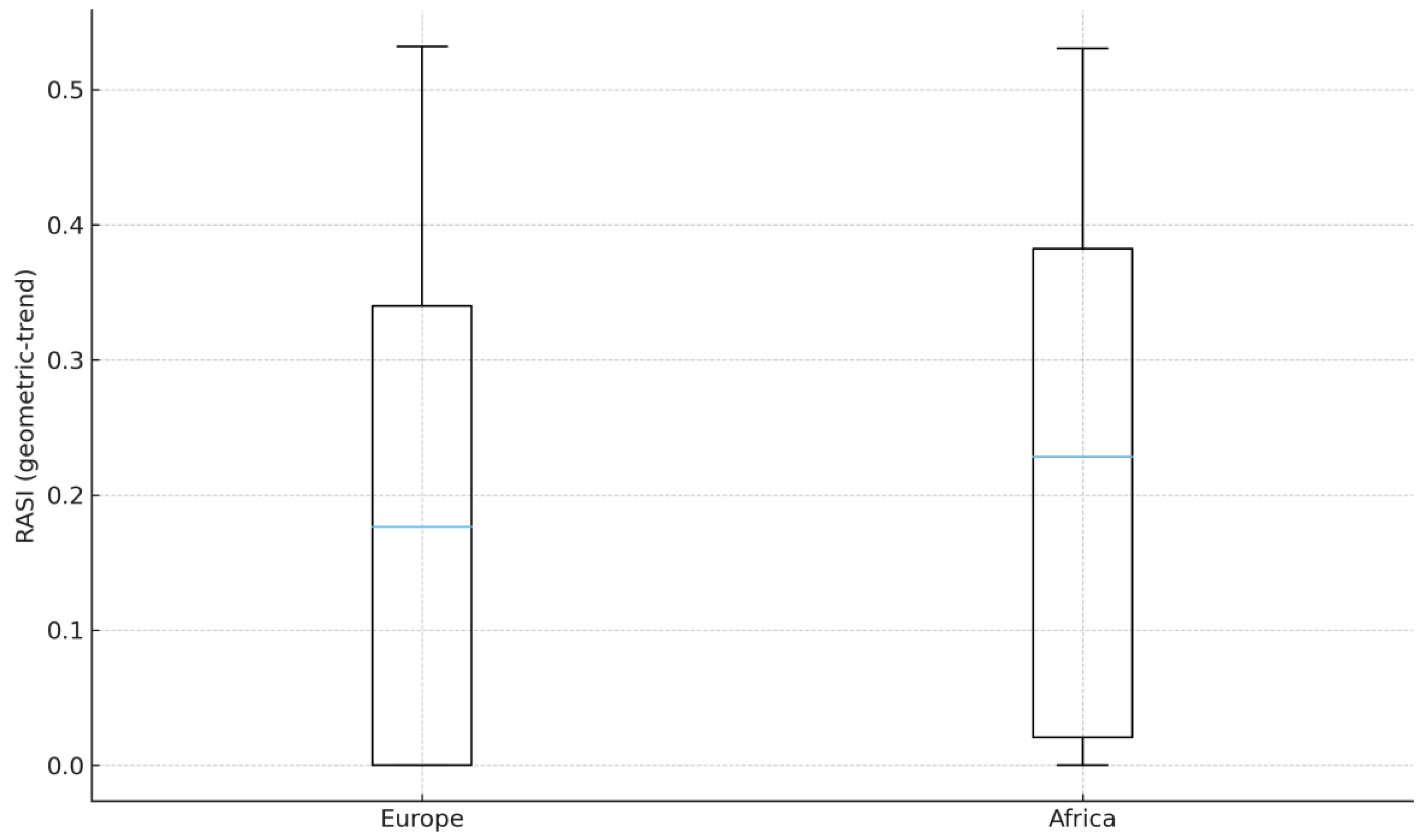
Figure 1.
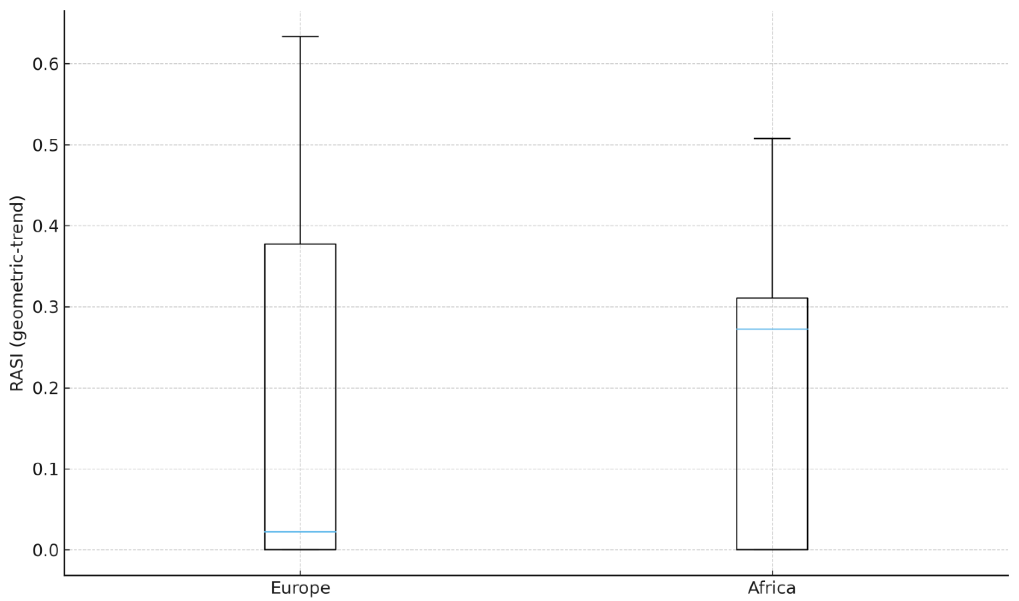
Distribution of country RASI by continent, 2007-2021. Source: Author’s calculation (based on World Bank DataBank data), 2025. Note: Ns: Africa 21, Europe 29 (inclusion ≥ 8 years). Geometric-trend baseline; risk = population SD of levels. Keep the interpretation in the text (do not include an “upper-tail” claim in the caption).
Figure 1.
Distribution of country RASI by continent, 2007-2021. Source: Author’s calculation (based on World Bank DataBank data), 2025. Note: Ns: Africa 21, Europe 29 (inclusion ≥ 8 years). Geometric-trend baseline; risk = population SD of levels. Keep the interpretation in the text (do not include an “upper-tail” claim in the caption).
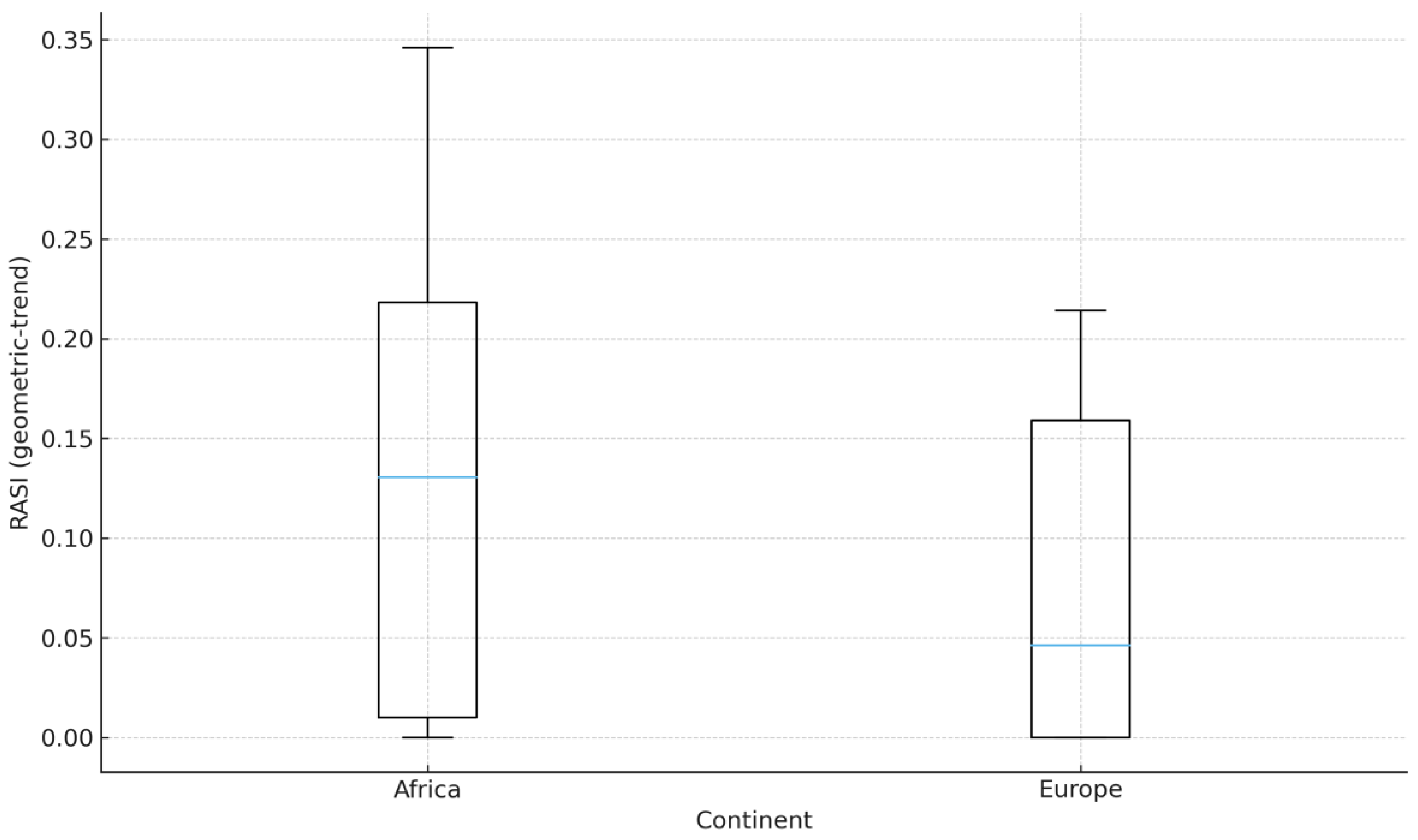
Figure 1 contrasts the continent-level RASI distributions for 2007-2021. Africa exhibited a higher median and wider interquartile range than Europe (Table 1: 0.131 vs. 0.046; 0.208 vs. 0.159), indicating a higher central tendency and greater cross-country dispersion. Continent-level ordering persists in the longer 2000-2021 window (Appendix Figure A1 and Table A1 and Table A3) and is robust to alternative risk normalizations (Figure 6), which corroborates a clear separation at the top (Figure 7, Figure 8, Figure 9 and Figure 10).
Figure 2.
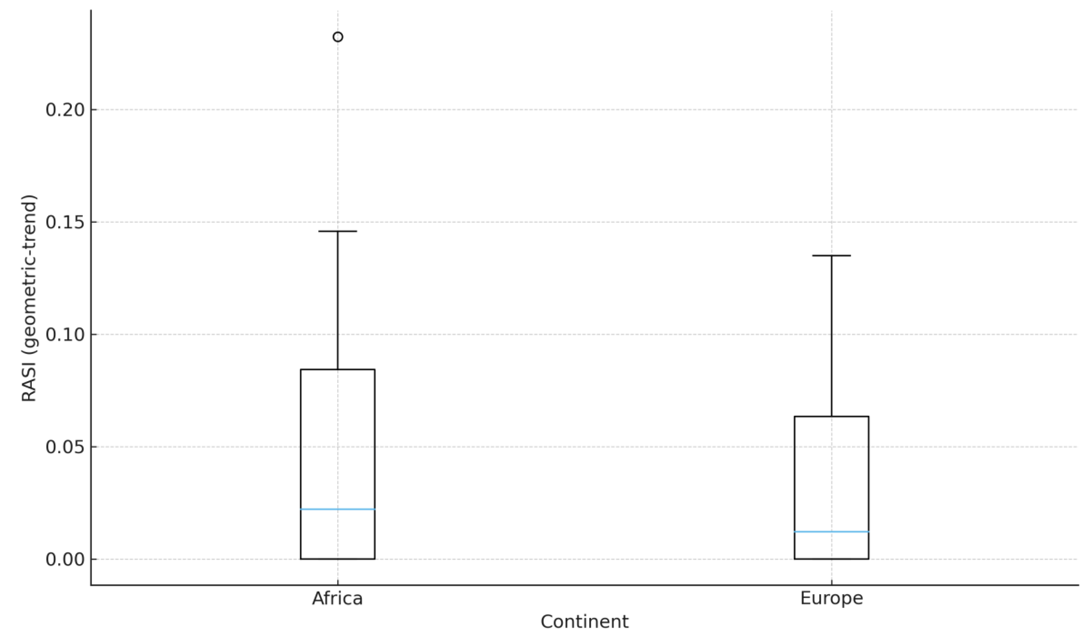
Europe: West vs East/Other country RASI, 2007-2021. Source: Author’s calculation (based on World Bank DataBank data), 2025. Notes: Ns: West 7, East/Other 22 (inclusion ≥ 8 years). Geometric-trend baseline; risk = population SD of levels.
Figure 2.
Europe: West vs East/Other country RASI, 2007-2021. Source: Author’s calculation (based on World Bank DataBank data), 2025. Notes: Ns: West 7, East/Other 22 (inclusion ≥ 8 years). Geometric-trend baseline; risk = population SD of levels.
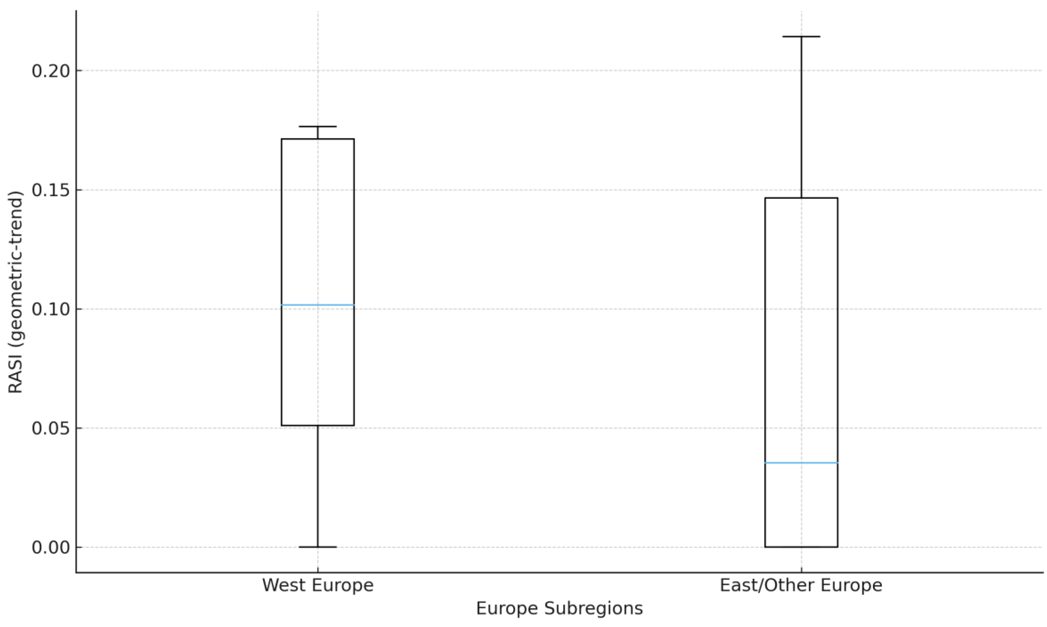
Within Europe, Western Europe’s distribution is shifted upward and exhibits tighter dispersion than that of East/Other Europe; the median and IQR are 0.102 vs. 0.035 and 0.120 vs. 0.147, respectively (Table 2). This is visually consistent with Figure 2, which also confirms the sample size (West = 7; East/Other = 22; inclusion ≥ 8 years). West > East/Other ordering persists in the extended window (Appendix Table A2 and Figure A2), supporting external validity beyond 2007-2021. Moreover, rank concordance is high across alternative risk normalizations (MAD-scaled, IQR-scaled, and downside semi-deviation), indicating that the result is not sensitive to the choice of dispersion metric (Figure 6). For the uncertainty context, bootstrap rank intervals and Top-1 probabilities (Figure 7, Figure 8, Figure 9 and Figure 10) indicate a clear separation at the top of Europe.
Figure 3.
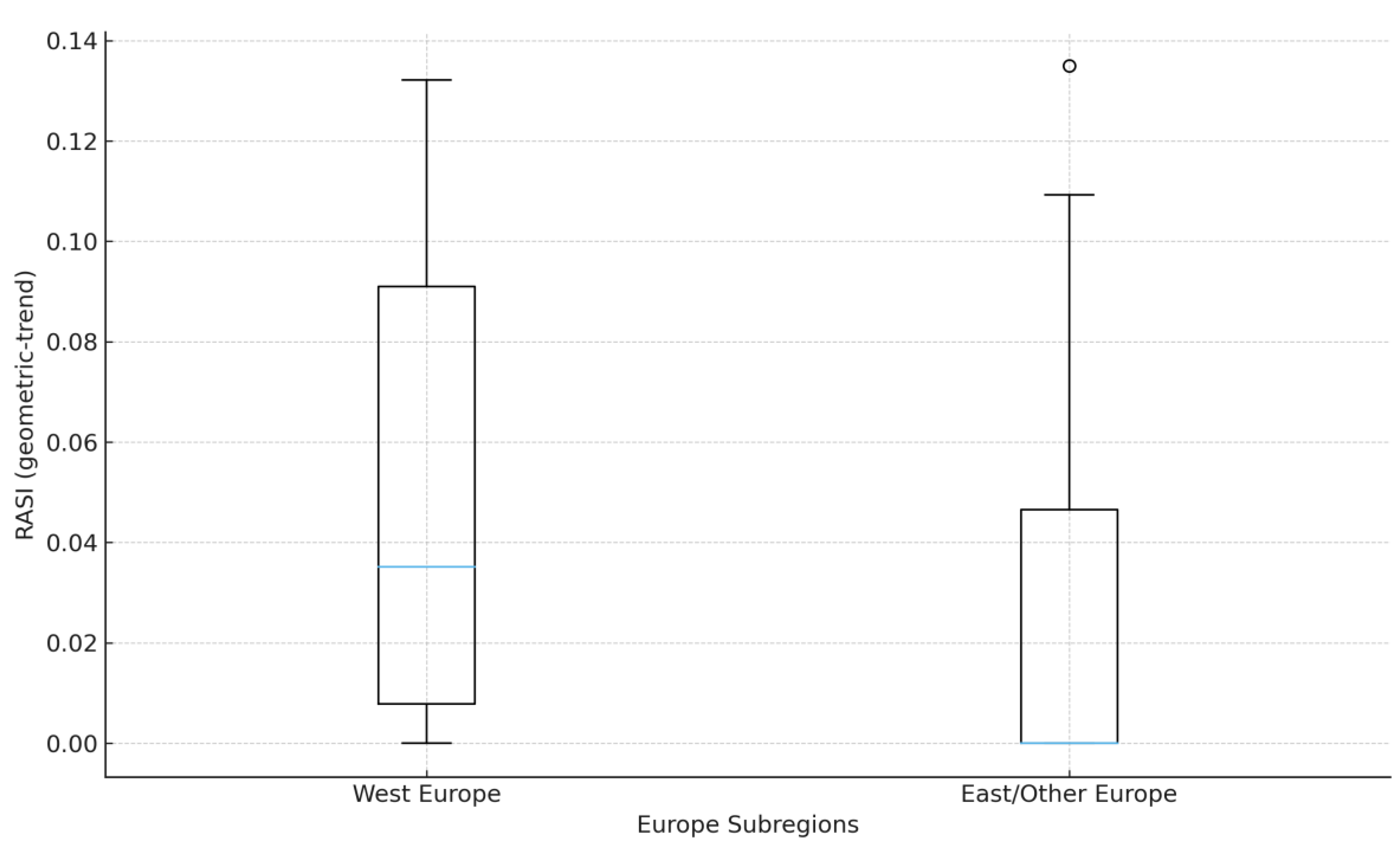
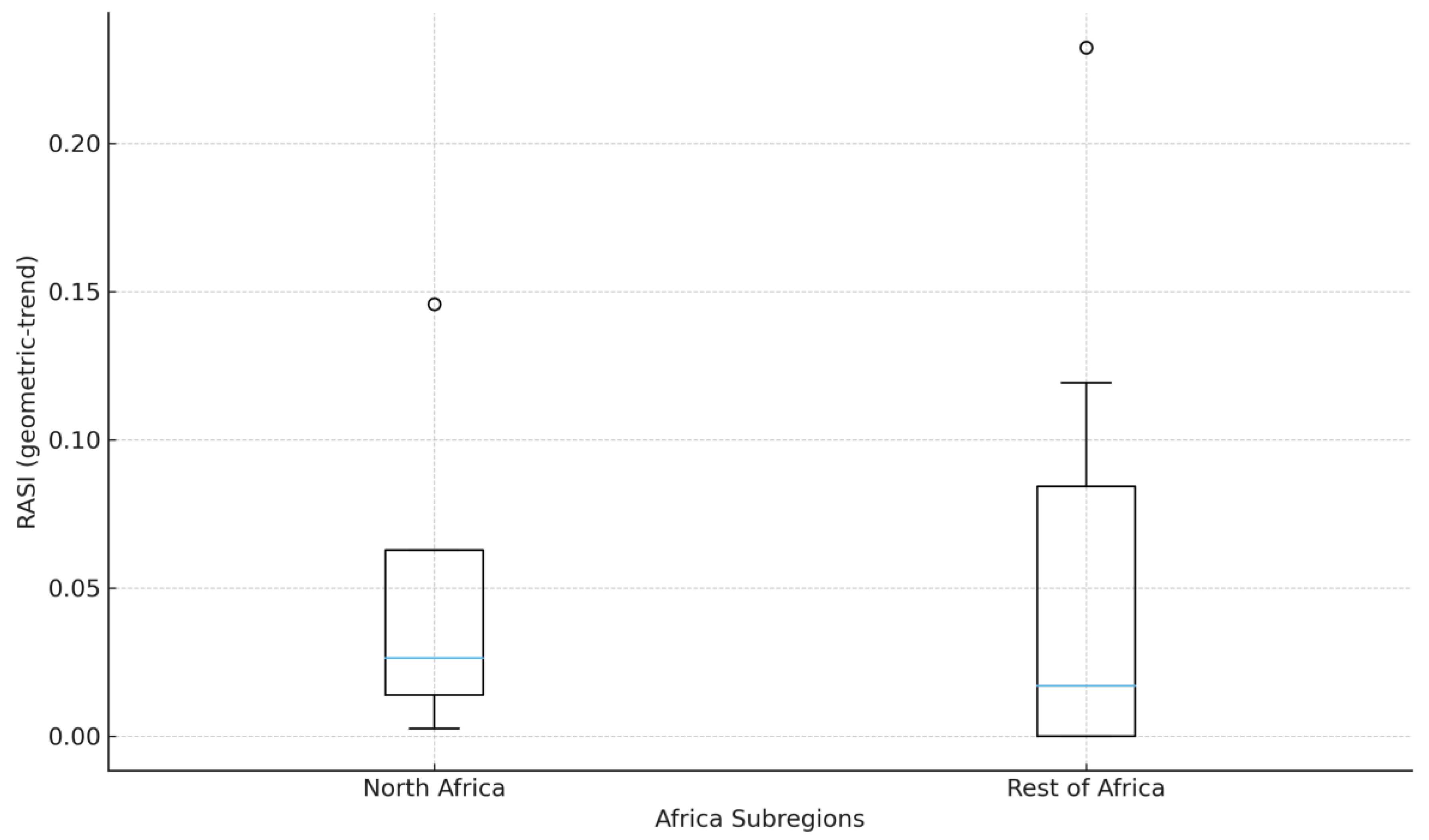
Africa: North vs Rest country RASI, 2007-2021. Source: Author’s calculation (based on World Bank DataBank data), 2025. Notes: Ns: North 4, Rest 17 (inclusion ≥ 8 years). Geometric-trend baseline; risk = population SD of levels.
Figure 3.
Africa: North vs Rest country RASI, 2007-2021. Source: Author’s calculation (based on World Bank DataBank data), 2025. Notes: Ns: North 4, Rest 17 (inclusion ≥ 8 years). Geometric-trend baseline; risk = population SD of levels.
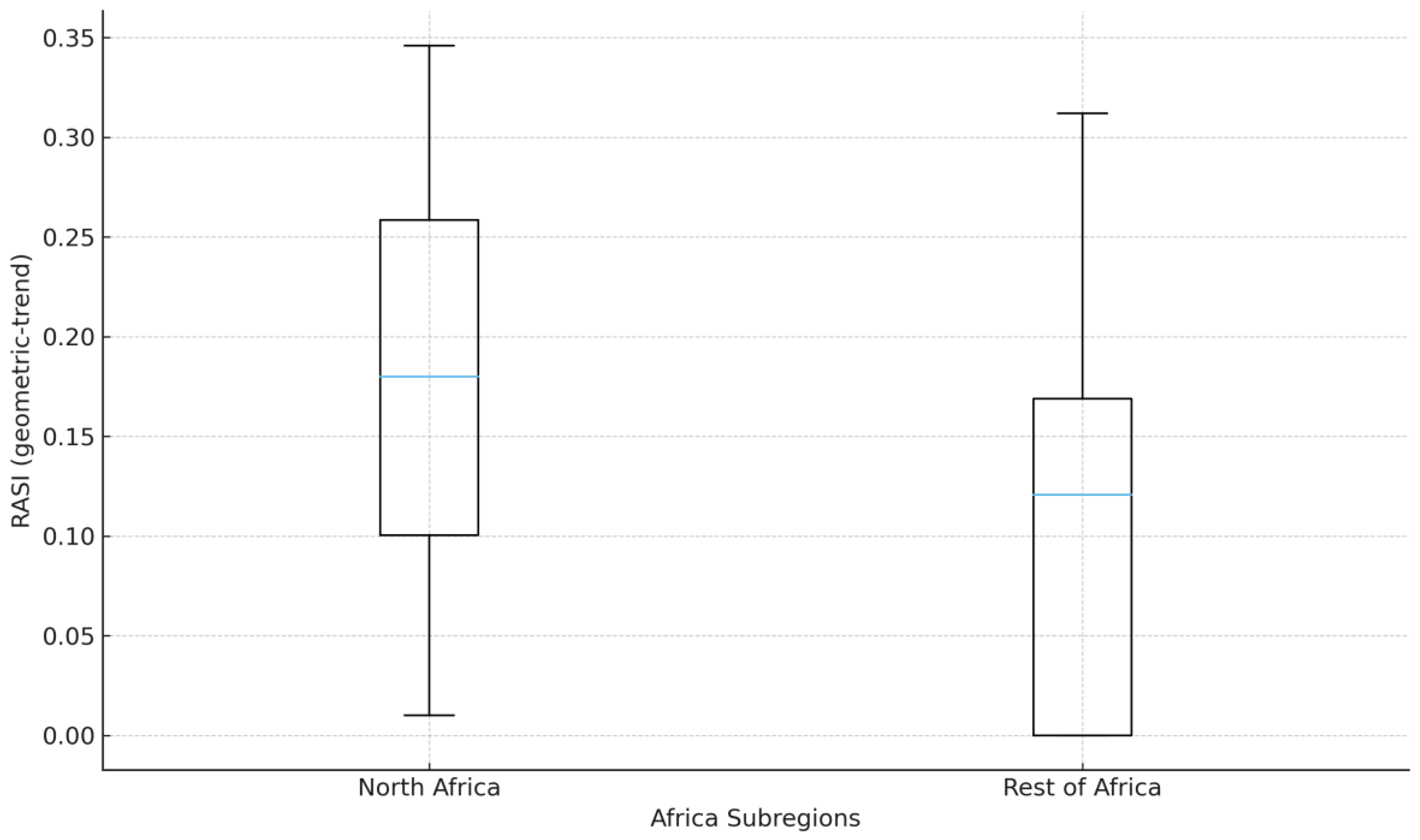
Within Africa, North Africa’s distribution is shifted upward relative to the Rest of Africa, with broadly similar dispersion; the median and IQR are 0.180 vs. 0.121 and 0.158 vs. 0.169, respectively (Table 3), indicating a difference in central tendency rather than spread. This is visually consistent with Figure 3, which confirms the sample sizes (North = 4; Rest = 17; inclusion ≥ 8) and baseline specification (geometric trend; risk = population SD). The ordering persists in the extended window (Appendix Table A2 and Figure A3), supporting external validity beyond the 2007-2021. Moreover, rank concordance is high under alternative risk normalizations (MAD-scaled, IQR-scaled, downside semi-deviation); therefore, the North vs Rest relation is not sensitive to the choice of dispersion metric (Figure 6). For the uncertainty context, bootstrap rank intervals and Top-1 leadership probabilities (Figure 7, Figure 8, Figure 9 and Figure 10) and jackknife stability (Figure 11) corroborate clear separation at the top without outsized sensitivity to single-year deletions; subperiod splits (Figure 12 and Figure 13) preserve ordering.
Figure 4.
Top 5 countries in Europe by RASI (geometric trend), 2007-2021. Source: Author’s calculation (based on World Bank DataBank data), 2025. Notes: See Figure 7 for bootstrap rank intervals; Ns: Europe 29 (inclusion age ≥ 8 years).
Figure 4.
Top 5 countries in Europe by RASI (geometric trend), 2007-2021. Source: Author’s calculation (based on World Bank DataBank data), 2025. Notes: See Figure 7 for bootstrap rank intervals; Ns: Europe 29 (inclusion age ≥ 8 years).
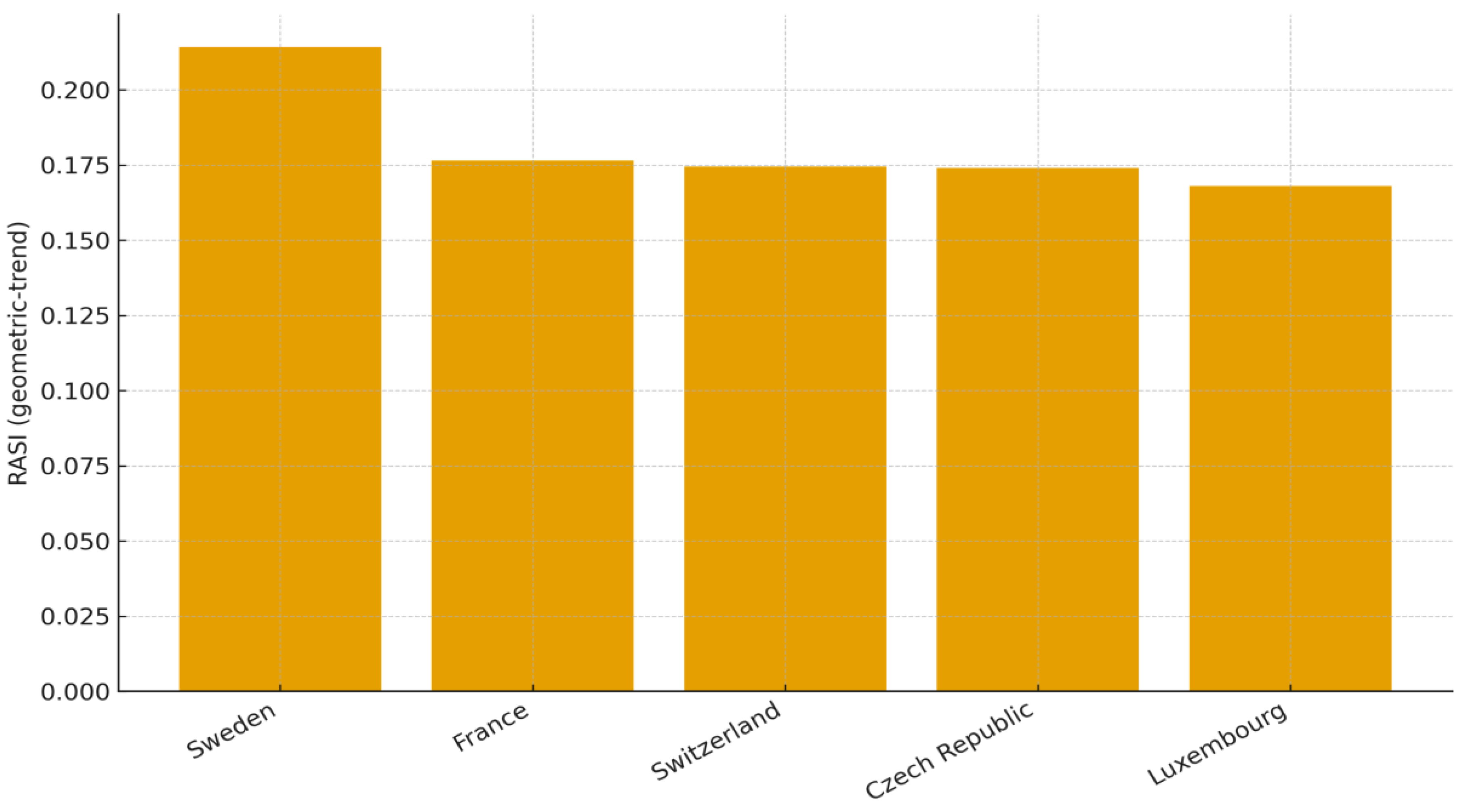
Within Europe, the Top-5 under the geometric-trend baseline (2007-2021) are Sweden, France, Switzerland, the Czech Republic, and Luxembourg (Figure 4). The common signature among these leaders is elevated average Z-score levels, credibly positive trend, and comparatively low volatility, consistent with the mechanics of RASI; the figure notes confirm Europe N = 29 with inclusion ≥ 8 years and direct readers to the uncertainty diagnostics. Precision and robustness: Bootstrap rank intervals are tight at the top (Figure 7), and under the Theil-Sen(log) trend, the identity of leaders and the overall stratification remain unchanged (Figure 8), indicating estimator-invariant leadership. Leadership probabilities concentrate on a small set of countries (Figure 9 and Figure 10), corroborating clear separation at the top, while rank concordance across alternative risk normalizations is very high in Europe (Spearman ρ ≈ 0.97-0.98), so conclusions are not sensitive to the dispersion metric (Figure 6). For stability to single-year deletions, jackknife CVs were low for the leaders (Figure 11). Taken together, in light of the broader within-Europe distributional gap (Table 2; Figure 2), these diagnostics support a durable Top-5 rather than a sample-specific artifact.
Figure 5.
Top-5 countries in Africa by RASI (geometric-trend), 2007-2021. Source: Author’s calculation (based on World Bank DataBank data), 2025. Notes: See Figure 7 for bootstrap rank intervals. Ns: Africa 21 (inclusion ≥ 8 years).
Figure 5.
Top-5 countries in Africa by RASI (geometric-trend), 2007-2021. Source: Author’s calculation (based on World Bank DataBank data), 2025. Notes: See Figure 7 for bootstrap rank intervals. Ns: Africa 21 (inclusion ≥ 8 years).
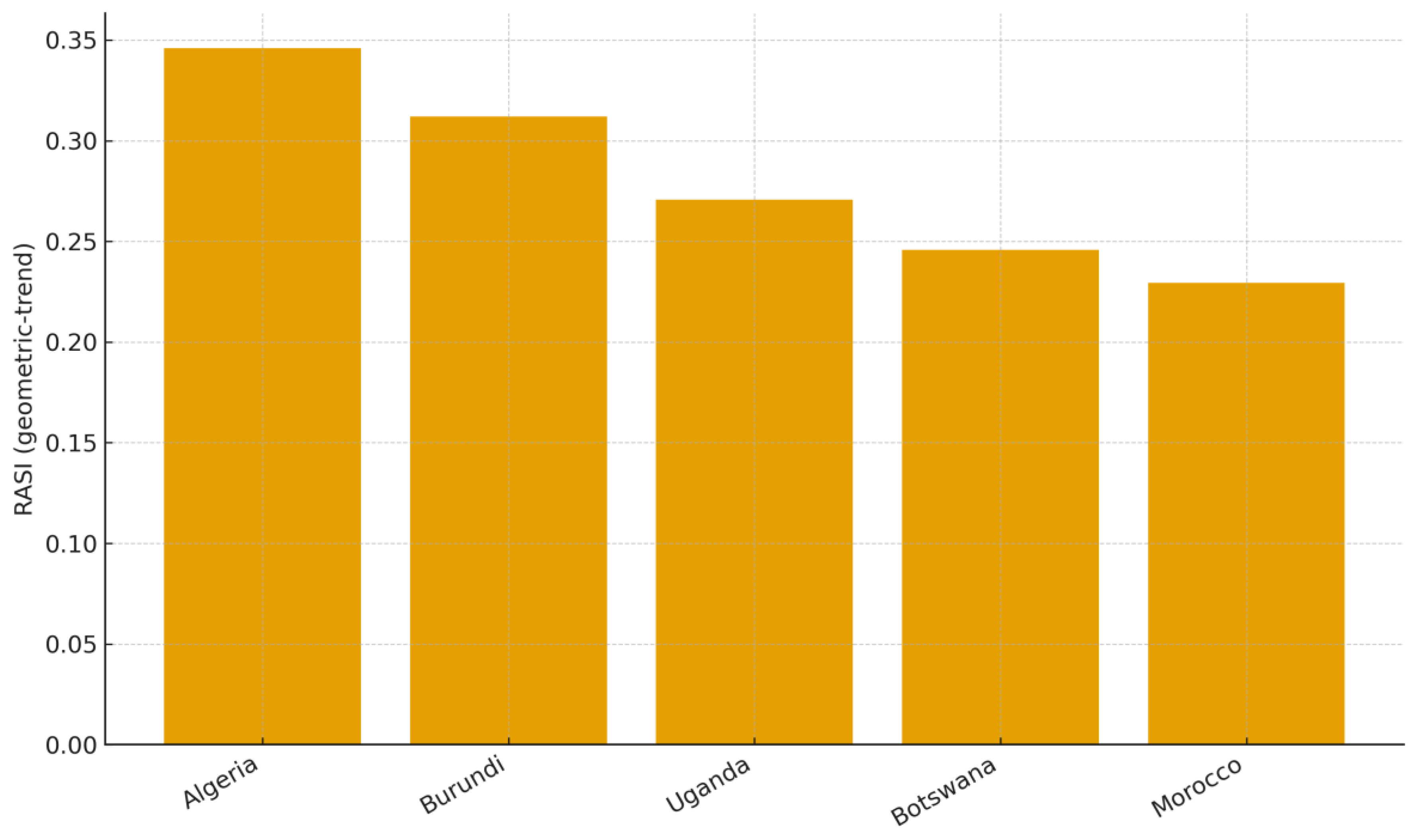
Within Africa, the Top-5 under the geometric-trend baseline (2007-2021) are Algeria, Burundi, Uganda, Botswana, and Morocco (Figure 5; Ns: Africa = 21; inclusion ≥ 8). The leadership pattern is consistent with RASI mechanics, elevated average Z-score levels, and non-negative (often positive) trends, scaled by contained dispersion, although the figure itself summarizes the composite rather than the components. Precision and robustness checks support these findings: bootstrap rank intervals are tight at the top (Figure 7) and remain under the Theil-Sen(log) trend (Figure 8), indicating estimator-invariant leadership. Top-1 leadership probabilities concentrate on a small set of countries (Figure 9 and Figure 10), corroborating clear separation at the top, while rank concordance across alternative risk normalizations is high in Africa (ρ≈0.90-0.93), so conclusions are not sensitive to the dispersion metric (Figure 6). For stability to single-year deletions, jackknife coefficients of variation were low for the leaders (Figure 11). Subperiod splits (2007-2013 and 2014-2021) preserve continent-level ordering, reinforcing external validity across regimes (Figure 12 and Figure 13).
3.1. Ranking Robustness and Stability
Figure 6.
Rank concordance across risk normalizations (Spearman ρ vs baseline, 2007-2021). Source: Author’s calculation (based on World Bank DataBank data), 2025. Notes: Spearman ρ computed within continent against baseline (population-SD) risk; alternatives: MAD-scaled, IQR-scaled, downside semi-deviation.
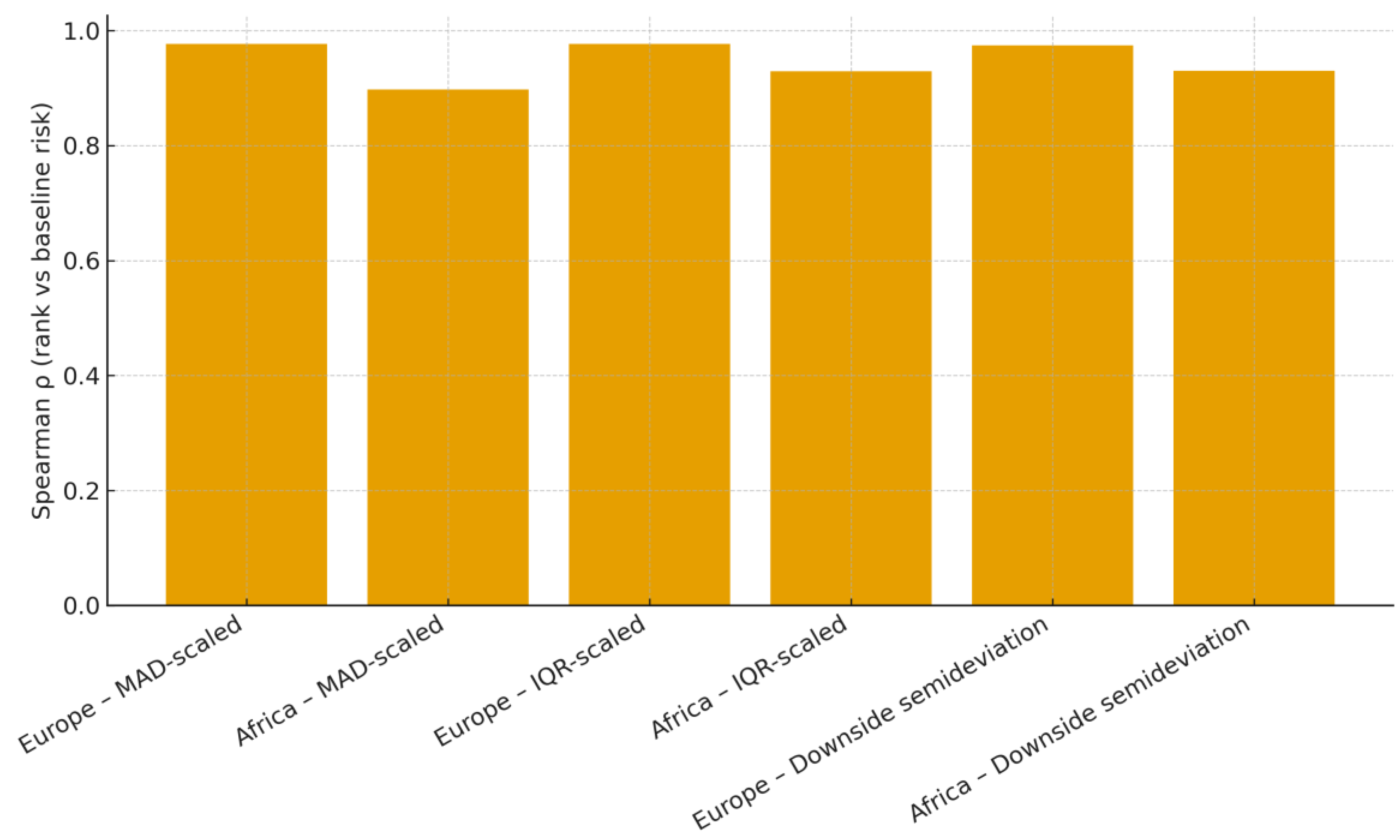
Rank concordance across alternative risk normalizations is high within continents, indicating that the ordering is largely invariant to the choice of the dispersion metric. In Europe, Spearman ρ versus the baseline (population-SD risk) is 0.98 (MAD-scaled), 0.98 (IQR-scaled), and 0.97 (downside semi-deviation); in Africa, it is 0.90, 0.93, and 0.93, respectively (Figure 6; notes: ρ computed within continent against the baseline). This aligns with the study design in which rank concordance is the primary check for risk-metric sensitivity (Methods §2.8; Algorithmic Summary step 8) and supports the interpretation of the baseline results as representative of reasonable alternatives. For the precision and stability context, see the bootstrap rank intervals and leadership probabilities (Figure 7, Figure 8, Figure 9 and Figure 10) and jackknife stability (Figure 11), which complement Figure 6 by quantifying uncertainty and year-deletion sensitivity.
Figure 7.
Bootstrap rank intervals - Geometric growth (B=1000; top 10 per continent). Source: Author’s calculation (based on World Bank DataBank data), 2025. Notes: Within-country, clustered bootstrap; Ns-Africa 21, Europe 29 (inclusion of ≥ 8 years). The intervals are the 5th–95th percentiles of the rank distributions.
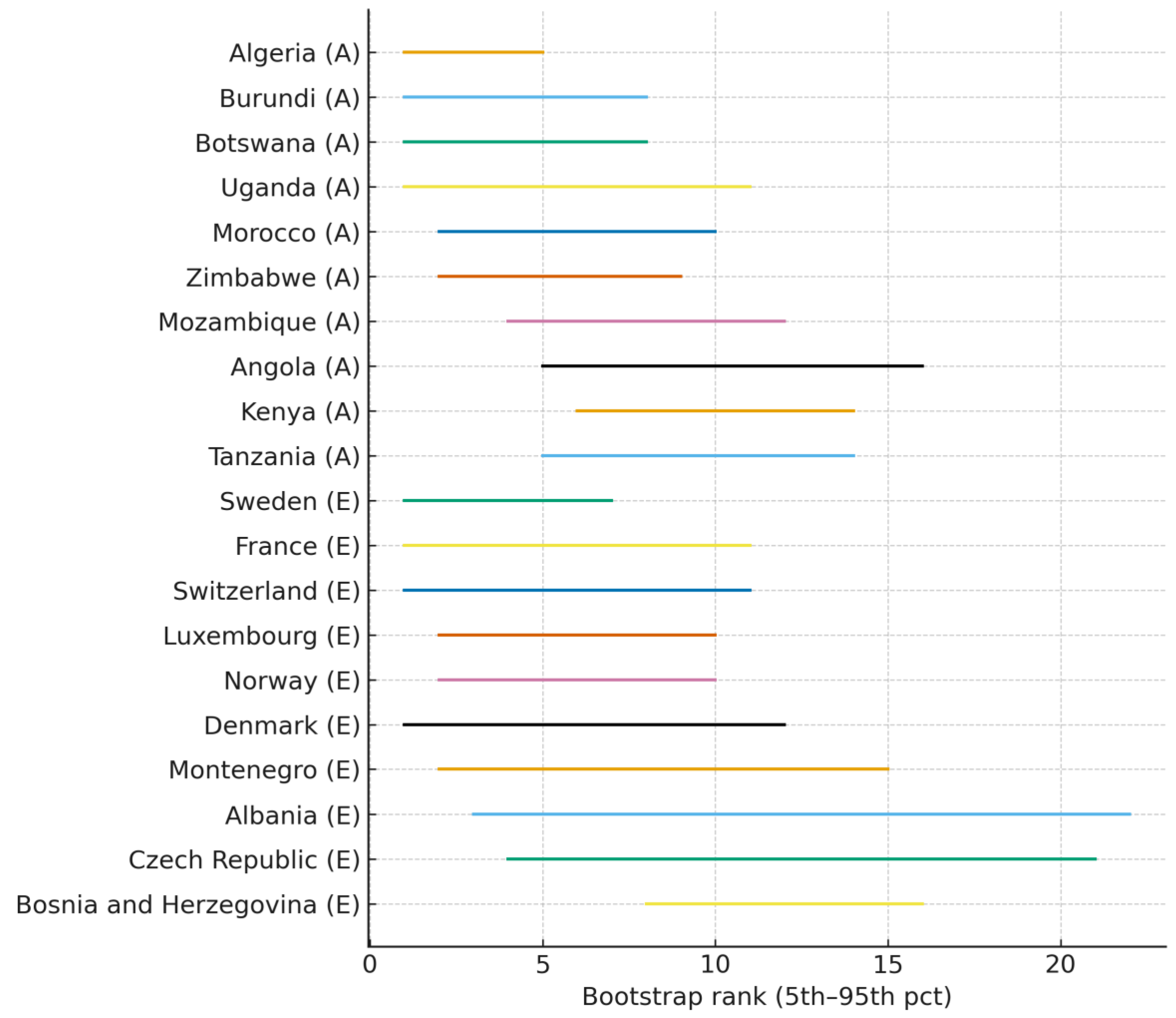
Bootstrap rank intervals (geometric trend) indicate a clear separation at the top and denser mid-ranking competition. Within a country, over-years clustered bootstrap with B = 1000 (seeded for reproducibility), 5th-95th percentile rank intervals for the Top-10 countries per continent are tight for leaders and widen lower in ranking, implying higher precision at the top and greater uncertainty among mid-ranked systems (Figure 7; Ns: Africa = 21, Europe = 29; inclusion ≥ 8 years). This diagnostic directly complements the methods in §2.5, and the algorithmic summary (step 6), which defines the clustered bootstrap and interval construction. Robustness across estimators is evident in Figure 8, where Theil-Sen(log) yields qualitatively similar intervals; leadership probabilities in Figure 9 and Figure 10 concentrate mass on a small set of countries, reinforcing the separation signaled by narrow top-rank intervals, and jackknife CVs in Figure 11 show that the top systems’ scores are not driven by single-year deletions.
Figure 8.
Bootstrap rank intervals Theil-Sen(log) growth (B=1000; top-10 per continent). Source: Author’s calculation (based on World Bank DataBank data), 2025. Notes: Within-country, clustered bootstrap; same sample as Figure 7.
Figure 8.
Bootstrap rank intervals Theil-Sen(log) growth (B=1000; top-10 per continent). Source: Author’s calculation (based on World Bank DataBank data), 2025. Notes: Within-country, clustered bootstrap; same sample as Figure 7.
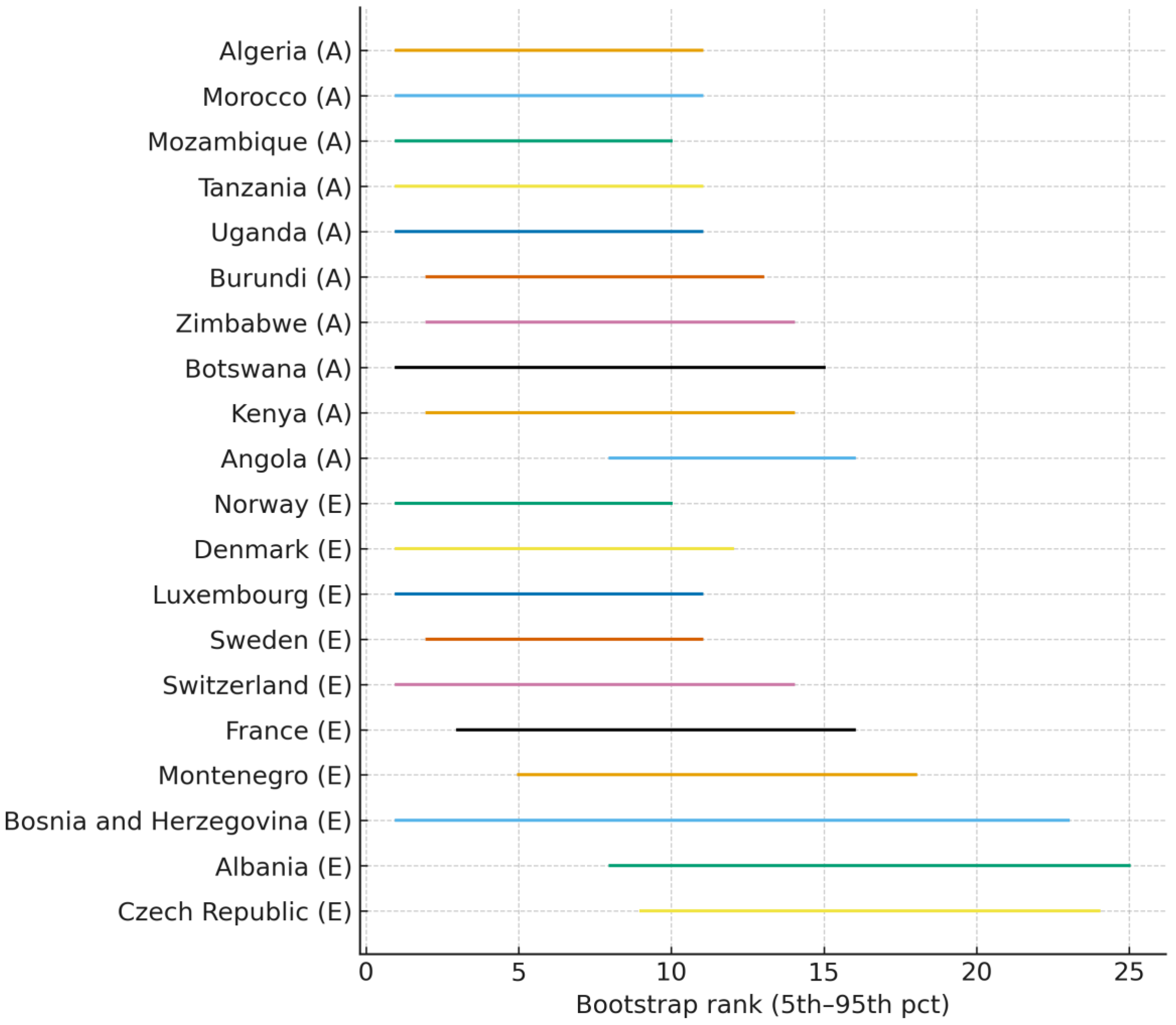
Bootstrap rank intervals under the Theil-Sen (log) trend confirm the geometric-baseline results. Using B=1000 within-country, over-years clustered resamples, the 5th-95th percentile rank intervals for the top 10 countries per continent closely matched those in Figure 7, and the identity of leaders and overall stratification remained unchanged (Figure 8; ns: Africa = 21, Europe = 29; inclusion ≥ 8 years). The Theil-Sen estimator’s endpoint robustness reduces sensitivity to idiosyncratic years, so the close agreement with the geometric version indicates estimator-invariant rankings rather than dependence on a particular trend metric. The resampling design follows methods §2.5, and the Algorithmic Summary (step 6), which defines the clustered bootstrap and rank-interval construction; Theil-Sen (log) is introduced in methods §2.2. In addition, leadership probabilities (Figure 9 and Figure 10) concentrate on a small set of countries, and jackknife stability (Figure 11) shows low CVs for leaders, both reinforcing the precision signaled by narrow top-rank intervals.
Figure 9.
Probability of Top-1 rank Geometric growth (B=1000; top-10 per continent). Source: Author’s calculation (based on World Bank DataBank data), 2025. Notes: Within-country, clustered bootstrap; Ns: Africa, 21; Europe, 29 (inclusion ≥ 8 years).
Figure 9.
Probability of Top-1 rank Geometric growth (B=1000; top-10 per continent). Source: Author’s calculation (based on World Bank DataBank data), 2025. Notes: Within-country, clustered bootstrap; Ns: Africa, 21; Europe, 29 (inclusion ≥ 8 years).
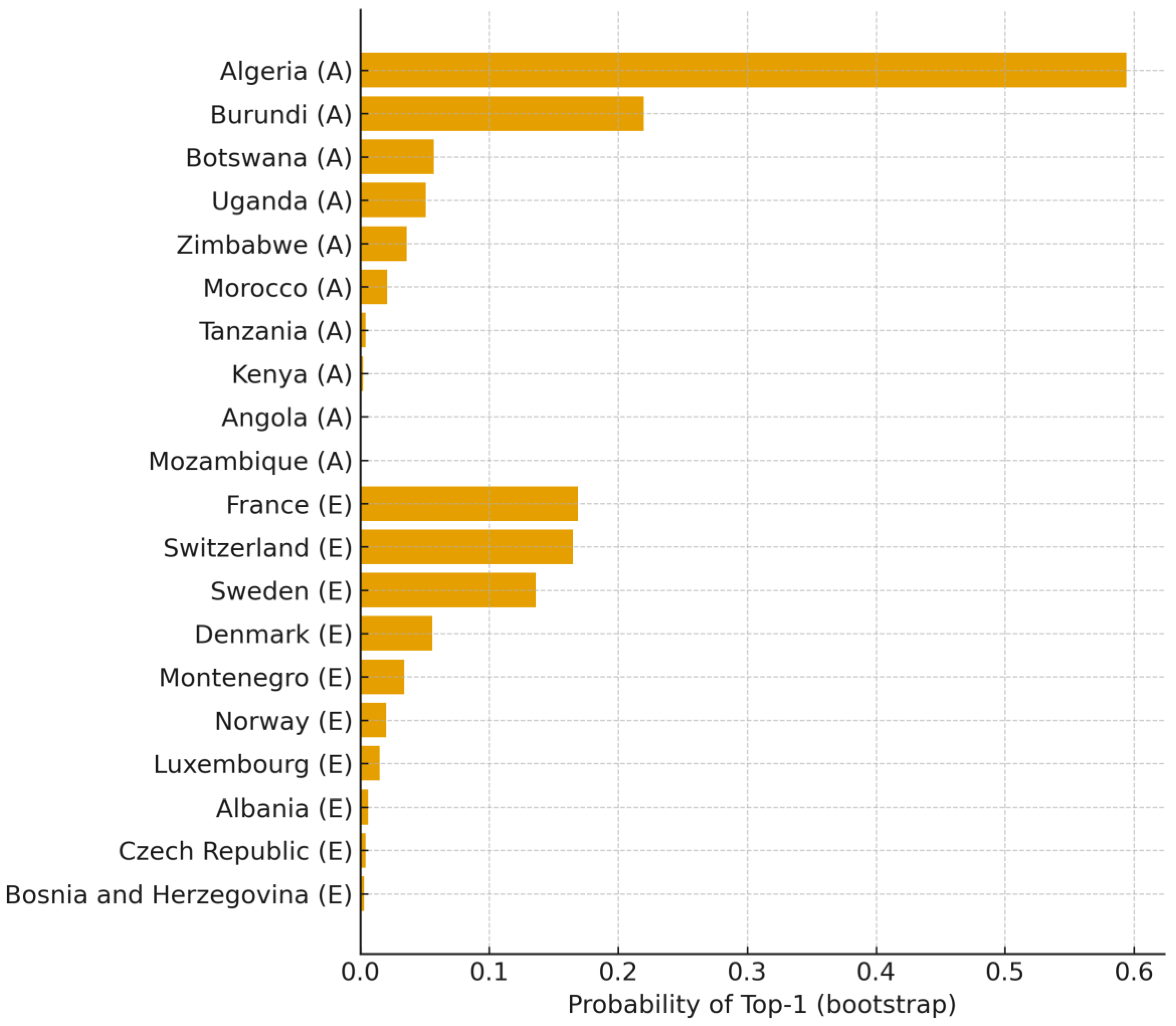
Top-1 leadership probabilities (geometric trend) are concentrated in a very small set of countries, with most others near zero. Using a within-country, over-years clustered bootstrap (B = 1000; Ns: Africa = 21, Europe = 29; inclusion ≥ 8 years), Figure 9 shows that only a handful of systems capture meaningful probability masses of P (rank= 1), implying a clear separation at the top. This pattern is consistent with the narrow top-rank intervals in Figure 7 and remains estimator-invariant under the Theil-Sen(log) trend (Figure 10). In the stability context, jackknife CVs are low for leading countries (Figure 11), and the sub-period splits (Figure 12 and Figure 13) preserve leadership ordering, reinforcing that these probabilities are not artifacts of a single period. The alignment with the Top-5 line-ups in Figure 4 and Figure 5 further corroborates that the countries with the highest Top-1 probabilities are the same ones that consistently lead the rankings.
Figure 10.
Probability of Top-1 rank Theil-Sen(log) (B=1000; top-10 per continent). Source: Author’s calculation (based on World Bank DataBank data), 2025. Notes: Within-country, clustered bootstrap; Ns: Africa, 21; Europe, 29 (inclusion ≥ 8 years).
Figure 10.
Probability of Top-1 rank Theil-Sen(log) (B=1000; top-10 per continent). Source: Author’s calculation (based on World Bank DataBank data), 2025. Notes: Within-country, clustered bootstrap; Ns: Africa, 21; Europe, 29 (inclusion ≥ 8 years).
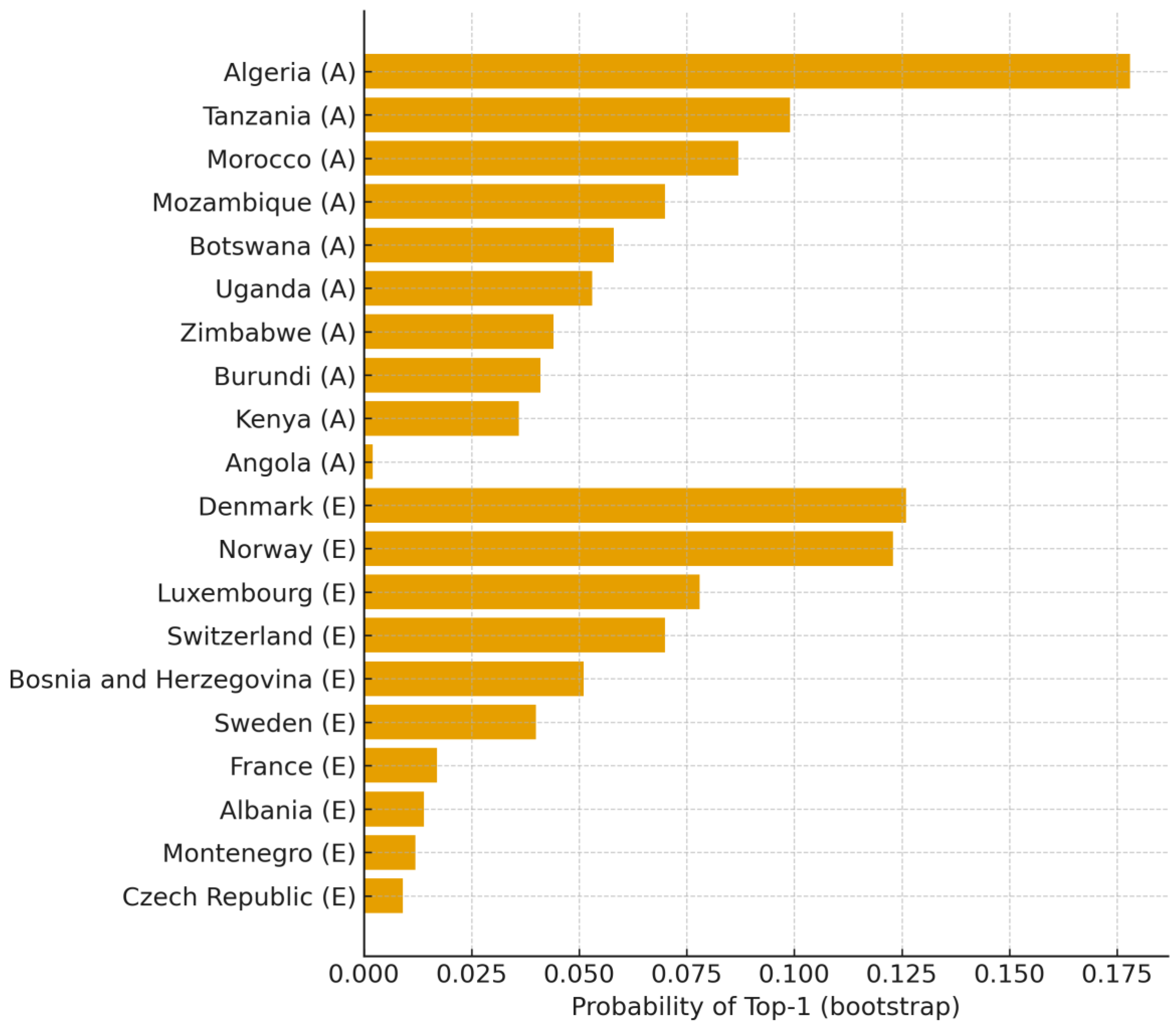
Top-1 leadership probabilities under the Theil-Sen(log) trend concentrate on a very small set of countries and closely mirror the geometric-trend benchmark, indicating that the identification of leading systems is estimator-invariant. Figure 10 was computed via a within-country, over-years clustered bootstrap (B = 1000; Ns: Africa = 21, Europe = 29; inclusion ≥ 8 years), the same design used for the geometric version in Figure 9. This aligns with the resampling protocol in the methods (clustered bootstrap and top-k probabilities; Algorithmic Summary step 6) and the role of Theil-Sen(log) as an endpoint-robust trend estimator. Consistency with the rank-interval diagnostics is evident: Figure 7 and Figure 8 show narrow top-rank intervals under both trend estimators, and the concentration of the Top-1 mass in Figure 10 reinforces this separation. For stability to single-year deletions, Figure 11 reports low jackknife CVs among leaders, supporting the durability of leadership probabilities.
Figure 11.
Jackknife Stability—Coefficient of Variation of Leave-One-Year-Out RASI (Geometric Baseline). Source: Author’s calculation (based on World Bank DataBank data), 2025. Notes: CV = sd(RASI_{−τ}) / mean(RASI_{−τ}); geometric-trend baseline.
Figure 11.
Jackknife Stability—Coefficient of Variation of Leave-One-Year-Out RASI (Geometric Baseline). Source: Author’s calculation (based on World Bank DataBank data), 2025. Notes: CV = sd(RASI_{−τ}) / mean(RASI_{−τ}); geometric-trend baseline.
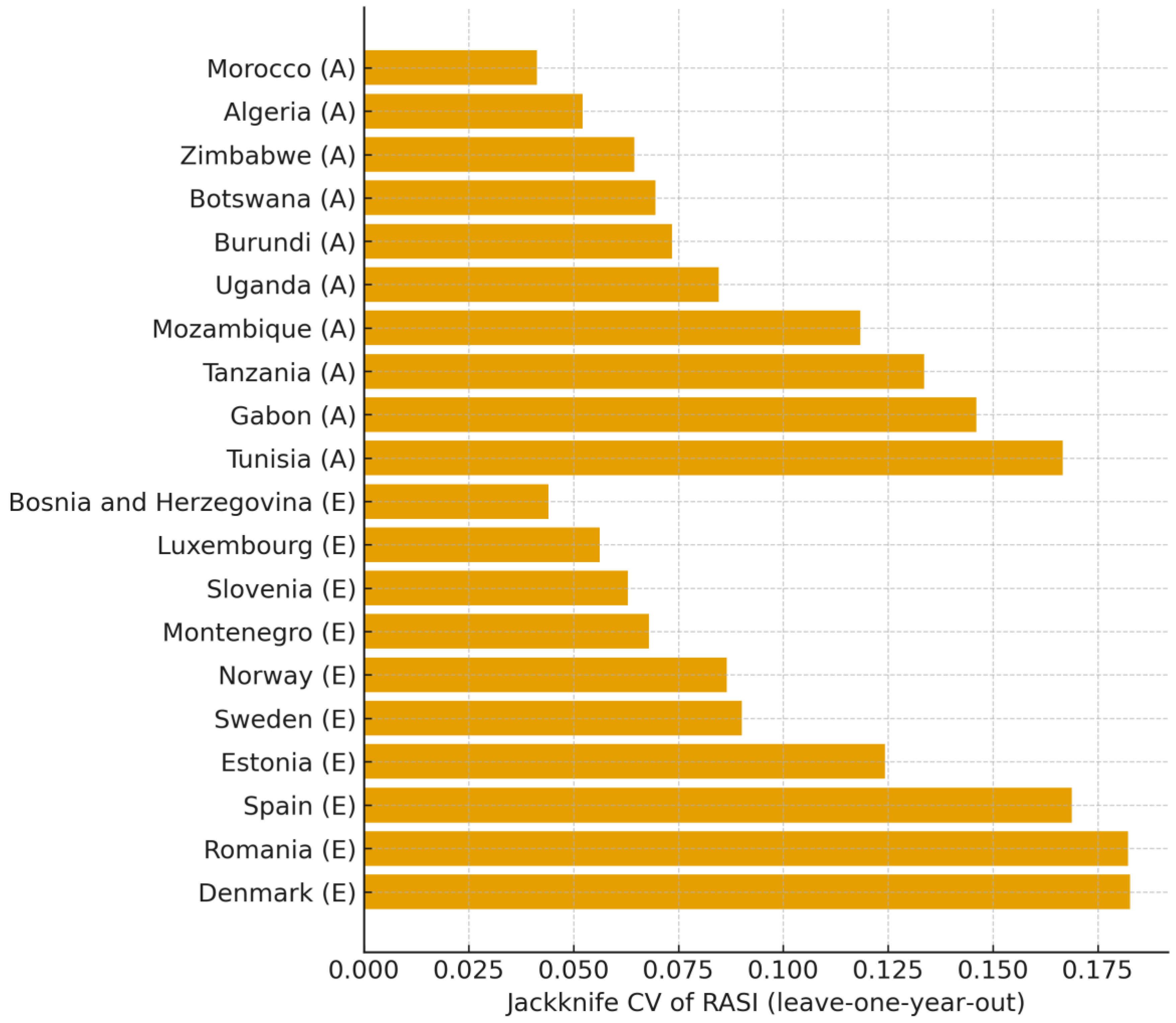
Jackknife stability indicates that top-ranked countries are not driven by single-year idiosyncrasies. Under the geometric-trend baseline, Figure 11 shows the coefficient of variation from a leave-one-year-out jackknife, CV = sd_τ(RASI_{−τ}) / mean_τ(RASI_{−τ}). Leaders show low CVs, while middle-rank countries exhibit higher CVs, implying greater sensitivity to episodic shocks. This diagnostic implements the protocol in Methods §2.6 and the Algorithmic Summary (step 7), and should be read alongside the bootstrap evidence on precision and leadership.
Cross-validation with other diagnostics. Narrow bootstrap rank intervals at the top (Figure 7) and their close match under Theil-Sen(log) (Figure 8) corroborate high precision for leaders; Top-1 leadership probabilities (Figure 9 and Figure 10) concentrate mass on a small set of countries, consistent with low jackknife CVs among those leaders. Subperiod splits (Figure 12 and Figure 13) preserve continent-level ordering, supporting external validity across regimes, and rank concordance under alternative risk normalizations (Figure 6) shows that conclusions are not sensitive to the dispersion metric.
Figure 12.
Subperiod RASI 2007-2013 (Geometric baseline; continent distributions). Source: Author’s calculation (based on World Bank DataBank data), 2025. Notes: Subperiod inclusion rule: ≥5 valid years.
Figure 12.
Subperiod RASI 2007-2013 (Geometric baseline; continent distributions). Source: Author’s calculation (based on World Bank DataBank data), 2025. Notes: Subperiod inclusion rule: ≥5 valid years.
Subperiod 2007-2013 preserves the full-sample continent ordering: Africa’s distribution remains above Europe’s, with wider dispersion consistent with crisis-period volatility, not a reversal of the hierarchy (Figure 12). The sub-period analysis applies the ≥ 5 valid-years inclusion rule (Methods §2.7), ensuring coverage while testing for invariance across regimes. This result is consistent with the 2007-2021 baseline (Table 1; Figure 1) and is corroborated by the 2014-2021 split (Figure 13), supporting external validity across distinct macro-financial environments; the same ordering also holds in the extended 2000-2021 window (Appendix Table A1, Table A2 and Table A3 and Figure A1, Figure A2 and Figure A3).
Figure 13.
Subperiod RASI 2014-2021 (Geometric baseline; continent distributions). Source: Author’s calculation (based on World Bank DataBank data), 2025. Notes: Subperiod inclusion rule: ≥5 valid years.
Figure 13.
Subperiod RASI 2014-2021 (Geometric baseline; continent distributions). Source: Author’s calculation (based on World Bank DataBank data), 2025. Notes: Subperiod inclusion rule: ≥5 valid years.
Subperiod 2014-2021 preserves the full-sample continent ordering, with Africa’s distribution remaining above Europe’s and only modest shifts in medians and IQRs relative to the baseline window (Figure 13). The sub-period analysis applies the ≥ 5 valid-years inclusion rule (Methods §2.7), ensuring coverage while testing for invariance across regimes. This result mirrors the 2007-2013 split (Figure 12) and is consistent with the 2007-2021 baseline (Table 1; Figure 1), supporting external validity beyond crisis-era conditions. The replication of the extended 2000-2021 window (Appendix Table A1, Table A2 and Table A3 and Figure A1, Figure A2 and Figure A3) corroborates the persistence of the cross-continental hierarchy. Complementary diagnostics, high within-continent rank concordance across risk normalizations (Figure 6), and bootstrap/jackknife evidence (Figure 7, Figure 8, Figure 9, Figure 10 and Figure 11), reinforce that these conclusions are insensitive to the dispersion metric and robust to sample variation.
4. Discussion
4.1. Cross-Continental Differences
Continent-level summaries indicate that Africa’s median RASI exceeds Europe’s over 2007-2021 (Table 1; Figure 1). Interquartile ranges are also wider in Africa, indicating greater middle-50-percent dispersion and cross-country heterogeneity (Table 1; Figure 1). Because RASI scales the mean level of the banking Z-score by a concave, non-negative transformation of trend and penalizes volatility in levels, the higher African median is consistent with favorable combinations of level and growth relative to dispersion. The extended 2000-2021 window preserves this ordering, reinforcing external validity beyond the crisis-era conditions (Appendix Table A1, Table A2 and Table A3 and Figure A1, Figure A2 and Figure A3). All interpretations refer to the baseline configuration (σ = population SD, φ(g) = log(1 + max {g, 0})). Reported rank intervals and leadership probabilities are derived from bootstrap-based rather than parametric confidence estimates, ensuring consistency with Algorithms 1-5.
4.2. Within-Continent Heterogeneity
Within Europe, Western Europe is shifted upward relative to East/Other Europe and exhibits tighter dispersion (Table 2; Figure 2). Within Africa, North Africa leads the Rest of Africa with broadly similar dispersion, indicating a shift in central tendency rather than outlier-driven spread (Table 3; Figure 3). Mechanistically, the observed subregional gaps align with a more favorable position on the RASI frontier, higher level, non-negative or positive trend, and lower dispersion among leaders relative to their regional peers.
4.3. Robustness and Uncertainty: What Each Diagnostic Adds
Three complementary diagnostics underpin the stability of these results. First, rank concordance across alternative risk normalizations (MAD-scaled, IQR-scaled, downside semi-deviation) is high within continents: Spearman ρ ≈ 0.98/0.98/0.97 in Europe and 0.90/0.93/0.93 in Africa; therefore, the ordering is not an artifact of a particular dispersion metric (Figure 6). Second, clustered bootstraps (B = 1000) deliver rank intervals and top-k leadership probabilities: intervals are tight at the top and widen middle-rank, while Top-1 mass concentrates on a small set of countries, both under the geometric and Theil-Sen(log) trends (Figure 7, Figure 8, Figure 9 and Figure 10). When useful, pairwise (or subregional) dominance can complement these summaries by reporting how often one unit’s RASI exceeds another in resamples. Third, jackknife stability shows low leave-one-year-out CVs for leaders, indicating that top standing is not driven by single-year idiosyncrasies (see Figure 11). Subperiod splits (2007-2013; 2014-2021) preserve ordering, further supporting the external validity (Figure 12 and Figure 13).
4.4. Economic Mechanisms and Interpretation
The RASI was decomposed into three interpretable dimensions. The level term reflects the baseline solvency/profitability embedded in the Z-score; the trend term, estimated via geometric-mean log-returns and Theil-Sen(log), rewards sustained improvement while mitigating endpoint sensitivity; the dispersion term penalizes volatility in levels, discouraging “growth via instability.” The concave link φ(g)=log(1+max{g,0}) ensures diminishing returns to a very high trend, and sets a non-positive trend to contribute zero. In this light, the superiority of West Europe over East/Other Europe and of North Africa over the Rest of Africa reflects higher baselines and steadier dynamics among leaders (Table 2 and Table 3; Figure 2 and Figure 3).
4.5. Policy and Portfolio Implications
The RASI provides a compact, auditable diagnostic of level trend-risk balance. The decomposition clarifies whether improvements are driven primarily by baseline levels, credible momentum, or reduced volatility, indicating where reforms may bind most. Within-continent benchmarking narrows the institutional heterogeneity and strengthens the relevance of cross-sectional comparisons for regional policy coordination. For allocators, continent and subregion medians summarize opportunity sets, leadership probabilities guide tilt magnitudes, jackknife CV can cap exposure to systems exhibiting instability under year deletion, and dominance can inform bilateral relative value calls. The results should be interpreted alongside the reported rank intervals and leadership probabilities to avoid overstating precision.
4.6. Limitations, Comparability, and Scope Conditions
RASI is descriptive, not structural: it ranks and benchmarks systems based on observed outcomes, without identifying causal channels. Cross-country heterogeneity in accounting and regulatory regimes and data coverage may be loaded into components. Mitigation is partial but salient: (i) benchmarking within continents, (ii) high within-continent rank concordance across dispersion metrics, and (iii) resampling diagnostics with surface sensitivity to idiosyncratic observations. Subperiod replication separates persistent relations from transitory noises.
4.7. Sensitivity and Forward-Looking Validation
Sensitivity checks vary the risk metric, trend estimator, inclusion thresholds, and time window; the conclusions are stable across these dimensions (Figure 6, Figure 7, Figure 8, Figure 9, Figure 10, Figure 11, Figure 12 and Figure 13; Appendix A). Future research could evaluate the predictive value of RASI in anticipating banking stress episodes or extend the framework to incorporate market-based measures of systemic risk, enhancing its role as an early-warning indicator.
5. Conclusions
This study introduces a transparent, reproducible Risk-Adjusted Stability Index that synthesizes the banking-system Z-score’s level, trend, and risk into a single, decision-useful measure for comparative benchmarking. In the main window (2007-2021), the cross-sectional hierarchy is clear, Africa’s median RASI exceeds that of Europe (0.131 vs. 0.046), and the same order holds within continents (West > East/Other Europe; North Africa > Rest). These statements are descriptive rather than causal and remain stable across estimators (geometric vs. Theil-Sen trends), alternative risk normalizations (MAD/IQR/downside), and uncertainty quantification via a within-country bootstrap (B=1000) and leave-one-year-out jackknife. Taken together, these findings indicate that the study’s objective is achieved: RASI provides transparent, uncertainty-aware, cross-country rankings that are robust across specifications and windows. Practically, the index’s decomposition clarifies whether relative standing is constrained by level, trend, or volatility, thereby supporting supervisory benchmarking and communication. The limitations include reliance on accounting-based Z-scores, omission of market-based tail risk, and interbank network effects. Future work should test out-of-sample usefulness, such as whether RASI helps flag subsequent stress episodes and expand coverage (more countries). In addition, future research could integrate RASI with market-based risk indicators or evaluate its predictive capacity for banking stress, extending its applicability in macroprudential policy.
Author Contributions
The author confirms sole responsibility for Conceptualization, Methodology, Software, Validation, Formal analysis, Investigation, Data curation, Visualization, Writing - original draft, writing - review and editing, and project administration.
Funding
This research received no external funding.
Institutional Review Board Statement
Not applicable.
Informed Consent Statement
Not applicable.
Data Availability Statement
The data presented in this study are available in Word Bank DataBank. These data were derived from the following resources available in the public domain: Global Financial DevelopmenDataBank (worldbank.org). All code used are available upon request.
Acknowledgments
ChatGPT (GPT-5 Thinking) was used as an assistive tool for the study analysis, figure/table templates, and English language editing.
Conflicts of Interest
The author declares no conflicts of interest.
Abbreviations
The following abbreviations are used in this manuscript:
| CV | Coefficient of Variation |
| IQR | Interquartile Range |
| MAD | Median Absolute Deviation |
| RASI | Risk-Adjusted Stability Index |
| SD | Standard Deviation |
Appendix A
This appendix replicates the continent and subregion comparisons over 2000-2021, maintaining the ≥8-observation inclusion rule. The main cross-sectional ordering is preserved (see also Appendix Table A1, Table A2 and Table A3 and Figure A1, Figure A2 and Figure A3). Specifications match main text (geometric-mean log-growth trend; baseline risk = population SD; inclusion ≥ 8). Extended-window medians are lower, consistent with the inclusion of earlier, weaker years; the cross-sectional ordering remains unchanged.

Table A1.
RASI by continent (2000-2021). Source: Author’s calculation (based on World Bank DataBank data), 2025.
Table A1.
RASI by continent (2000-2021). Source: Author’s calculation (based on World Bank DataBank data), 2025.
| Continent | Countries | Median RASI (geo) | IQR (geo) |
|---|---|---|---|
| Africa | 22 | 0.022 | 0.084 |
| Europe | 29 | 0.012 | 0.063 |
Notes: Specifications are identical to the main text (geometric trend; φ as above; risk = population SD; inclusion ≥ 8).
Extending the window to 2000-2021 corroborates the main findings: Africa’s median remains above that of Europe (0.022 vs. 0.012). A longer horizon integrates more business cycle variation without overturning cross-continental ordering.
Table A2.
Subregion comparisons, 2000-2021. Source: Author’s calculation (based on World Bank DataBank data), 2025.
Table A2.
Subregion comparisons, 2000-2021. Source: Author’s calculation (based on World Bank DataBank data), 2025.
| Continent | Subregion | Countries | Median RASI (geo) | IQR (geo) |
|---|---|---|---|---|
| Europe | West Europe | 7 | 0.035 | 0.083 |
| Europe | East/Other Europe | 22 | 0.000 | 0.047 |
| Africa | North Africa | 4 | 0.026 | 0.049 |
| Africa | Rest of Africa | 18 | 0.017 | 0.084 |
Notes: The zero median in East/Other Europe reflects φ(g)=0 for a non-positive trend; ordering robust under Theil-Sen; see Figure 6.
Subregion comparisons for 2000-2021 preserve the main relations: West Europe exceeds East/Other Europe, and North Africa exceeds the Rest of Africa. Persistence across windows indicates out-of-period robustness and generalizability over time rather than period-specific patterns.
Table A3.
Medians: 2007-2021 vs 2000-2021. Source: Author’s calculation (based on World Bank DataBank data), 2025.
Table A3.
Medians: 2007-2021 vs 2000-2021. Source: Author’s calculation (based on World Bank DataBank data), 2025.
| Continent | Median (2007–2021) | Median (2000–2021) |
|---|---|---|
| Africa | 0.131 | 0.022 |
| Europe | 0.046 | 0.012 |
Notes: Lower extended-window medians reflect earlier weaker years; ordering unchanged.
A side-by-side comparison of medians and IQRs indicates that extending the horizon modestly reduces dispersion, while leaving the cross-continental ranking unchanged. The persistence of ordering across windows provides out-of-period robustness and supports the generalizability over time.
Figure A1.
Distribution of country RASI by continent, 2000-2021. Source: Author’s calculation (based on World Bank DataBank data), 2025. Notes: Specification identical to the main text (geometric trend, population-SD risk, inclusion ≥ 8).
Figure A1.
Distribution of country RASI by continent, 2000-2021. Source: Author’s calculation (based on World Bank DataBank data), 2025. Notes: Specification identical to the main text (geometric trend, population-SD risk, inclusion ≥ 8).
The longer (2000-2021) window preserves the relative positions of the two continents and slightly narrows dispersion, consistent with averaging over a longer horizon (more business-cycle states).
Figure A2.
Europe: West vs East/Other country RASI, 2000-2021. Source: Author’s calculation (based on World Bank DataBank data), 2025. Notes: Specification identical to main text.
Figure A2.
Europe: West vs East/Other country RASI, 2000-2021. Source: Author’s calculation (based on World Bank DataBank data), 2025. Notes: Specification identical to main text.
The West-East/Other differential is robust to the extended 2000-2021 horizon, consistent with persistent cross-subregional differences in level, trend, and dispersion.
Figure A3.
Africa: North vs Rest country RASI, 2000-2021. Source: Author’s calculation (based on World Bank DataBank data), 2025. Notes: Specification identical to main text.
Figure A3.
Africa: North vs Rest country RASI, 2000-2021. Source: Author’s calculation (based on World Bank DataBank data), 2025. Notes: Specification identical to main text.
North Africa maintains its advantage over the Rest of Africa at the median, indicating a higher central tendency. The dispersion is broadly similar, suggesting that the results are not driven by outliers.
References
- Albulescu, C.T. (2013). Financial Stability and Monetary Policy: A Reduced-Form Model for the EURO Area. Journal for Economic Forecasting, vol. 16, no. 1, pp. 62–81.
- Boubaker, S., Ngo, T., Samitas, A. Tripe, D. (2024). An MCDA composite index of bank stability using CAMELS ratios and shannon entropy. Annals of Operational Research. Available at: https://doi.org/10.1007/s10479-024-06023-3 (Retrieved 07/15/2025). [CrossRef]
- Demirguc-Kent, A. and E. Detragiache (1998). "Financial liberalization and financial fragility". Policy Research Working Paper Series 1917. The World Bank.
- Gulati, R., Hassan, M.K. & Charles, V. (2024). Developing a New Multidimensional Index of Bank Stability and Its Usage in the Design of Optimal Policy Interventions. Comput Econ 63, 1281–1325. Available at: https://doi.org/10.1007/s10614-023-10401-7 (Retrieved 08/15/2025). [CrossRef]
- Holló, D., Kremer, M., & Duca, M L. (2012). CISS a composite indicator of systemic stress in the financial system. ECB. Working paper series 1426. March. Available at: https://www.ecb.europa.eu/pub/pdf (Retrieved 07/05/2025).
- Jide, L. (2003). An Early Warning Model of Bank Failure in Jamaica: An Information Theoretic Approach‖. Financial Stability Department, Bank of Jamaica.
- Kočišová, K. (2015). Banking Stability Index: A Cross-Country Study. Available at:(PDF) Banking Stability Index: A Cross-Country Study (Retrieved 07/25/2025).
- Paradi, J., and Zhu, H. (2013). A survey on bank branch efficiency and performance research with data envelopment analysis. OMEGA, 41(1), 61–79. [CrossRef]
- Petrović, D., Dasilas, A., Karanovic, G. (2025). Bank risk-adjusted efficiency using a composite risk management index. The Journal of Risk Finance 26(3): 485–515.Available at: https://doi.org/10.1108/JRF-11-2024-0362 (Retrieved 07/10/2025). [CrossRef]
- World Bank, DataBank, 2025. Global Financial Development. Available at: Global Financial DevelopmenDataBank (worldbank.org) (Retrieved 08/02/2025).
Table 1.
RASI by continent (2007-2021). Source: Author’s calculation (based on World Bank DataBank data), 2025.
Table 1.
RASI by continent (2007-2021). Source: Author’s calculation (based on World Bank DataBank data), 2025.
| Continent | Countries | Median RASI (geo) | IQR (geo) | Median RASI (TS) |
|---|---|---|---|---|
| Africa | 21 | 0.131 | 0.208 | 0.125 |
| Europe | 29 | 0.046 | 0.159 | 0.117 |
Note: Medians represent geometric-trend specification. The last column reports Theil–Sen(log) medians. φ(g) = log(1 + max{g, 0}); risk = population SD of Z-score levels; inclusion ≥ 8 annual observations.
Table 2.
Europe: West vs East/Other, 2007-2021. Source: Author’s calculation (based on World Bank DataBank data), 2025.
Table 2.
Europe: West vs East/Other, 2007-2021. Source: Author’s calculation (based on World Bank DataBank data), 2025.
| Subregion | Countries | Median RASI (geo) | IQR (geo) |
|---|---|---|---|
| West Europe | 7 | 0.102 | 0.120 |
| East/Other Europe | 22 | 0.035 | 0.147 |
Note: Ordering is preserved under Theil-Sen(log); see Figure 6 for within-continent rank concordance across risk normalizations.
Table 3.
Africa: North vs Rest, 2007-2021. Source: Author’s calculation (based on World Bank DataBank data), 2025.
Table 3.
Africa: North vs Rest, 2007-2021. Source: Author’s calculation (based on World Bank DataBank data), 2025.
| Subregion | Countries | Median RASI (geo) | IQR (geo) |
|---|---|---|---|
| North Africa | 4 | 0.180 | 0.158 |
| Rest of Africa | 17 | 0.121 | 0.169 |
Note: Theil-Sen medians (not shown) preserve ordering; see Figure 6 for within-continent rank concordance.
Disclaimer/Publisher’s Note: The statements, opinions and data contained in all publications are solely those of the individual author(s) and contributor(s) and not of MDPI and/or the editor(s). MDPI and/or the editor(s) disclaim responsibility for any injury to people or property resulting from any ideas, methods, instructions or products referred to in the content. |
© 2025 by the author. Licensee MDPI, Basel, Switzerland. This article is an open access article distributed under the terms and conditions of the Creative Commons Attribution (CC BY) license (https://creativecommons.org/licenses/by/4.0/).
Copyright: This open access article is published under a Creative Commons CC BY 4.0 license, which permit the free download, distribution, and reuse, provided that the author and preprint are cited in any reuse.


