
Submitted:
17 October 2025
Posted:
20 October 2025
You are already at the latest version
Abstract
Hyperspectral remote sensing imagery provides invaluable information for environmental and agricultural monitoring but remains highly susceptible to atmospheric haze. We introduce the first comprehensive benchmark for hyperspectral image dehazing featuring paired real-world hazy and haze-free remote sensing data. The Remote sensing Real-world Hyperspectral Paired Dehazing Image Dataset (RRealHyperPDID) includes 110 scenes with naturally occurring haze and corresponding clear references, enabling reliable evaluation of dehazing algorithms across both hyperspectral and RGB domains. To support model training and ablation studies, we present the Remote Sensing Synthetic Hyperspectral Paired Dehazing Image Dataset (RSyntHyperPDID), comprising 2,616 synthetically generated hazy-clear pairs. The benchmark also provides agricultural field delineation annotations, allowing assessment of dehazing effects on downstream remote sensing tasks. Extensive experiments with six state-of-the-art methods reveal fundamental limitations of existing hyperspectral dehazing approaches and highlight the need for realistic, domain-consistent data. Models trained on RSyntHyperPDID demonstrate better generalization to real hazy data, establishing a new baseline for hyperspectral dehazing.
Keywords:
hyperspectral image (HSI)
; remote sensing
; dehazing benchmark
; real-world dehazing
; agricultural field delineation
1. Introduction
Haze complicates image analysis and adversely affects the performance of machine vision systems [1,2]. The haze effect results from the partial absorption and scattering of light reflected from the scene as it travels through the turbid medium between the scene and the sensor. The goal of dehazing is to reconstruct the scene as it would appear under haze-free conditions, given only the hazy observation.
Classical dehazing techniques are based on physical models of haze formation combined with simplifying assumptions, such as the dark channel prior, which assumes the existence of near-zero intensity values in local haze-free image patches [3] and others [4,5,6,7]. In recent years, deep learning methods have been introduced for dehazing, ranging from early convolutional neural networks (CNNs) such as FFANet [8], RSDehazeNet [9], and CANet [10], to transformer-based architectures like DehazeFormer [11], AIDTransformer [12], and RSDformer [13]. The latest Mamba-based models, such as RSDehamba [14] and HDMba [15], have claimed improved capability to capture spatially varying haze distribution.
Developing and evaluating dehazing algorithms requires datasets containing paired hazy and haze-free images of the same scene. However, haze is a difficult-to-reproduce and poorly controlled imaging condition. For ground-based image dehazing, open-source datasets with haze-free references and real haze generated by haze machines are available [16], but this approach is infeasible for remote sensing image dehazing (RSID).
For RSID, only unpaired datasets with real haze have been available so far, lacking corresponding clean reference images [11]. To compensate for this, haze augmentation has become a common practice: haze is synthetically applied to clear remote sensing images using physical or empirical models. However, the quality of the augmentation model critically affects the realism of the generated data. For example, [17] demonstrated that imperfections in the haze synthesis model can cause noticeable brightness loss in augmented images. Thus, synthetic augmentation can only serve as a complementary tool and cannot fully replace real paired data [18]. Until recently, no dataset of paired hazy and haze-free remote sensing images existed. The first such dataset, Real-World Remote Sensing Hazy Image Dataset (RRSHID), containing RGB image pairs derived from multispectral satellite data, was introduced in 2025 [18].
Dehazing hyperspectral images (HSIs) presents unique challenges. Compared to RGB imagery, HSIs capture rich spectral information, offering considerable potential for downstream remote sensing tasks. While several specialized HSI dehazing methods have been proposed [8,12,15,19], evaluating their real-world performance remains difficult due to the absence of paired hyperspectral datasets with real haze. Unlike multispectral imagery, hyperspectral remote sensing data are expensive and technically complex to acquire. No dataset comparable to RRSHID currently exists for the hyperspectral domain. Moreover, there are no standardized haze-augmented benchmarks with defined train–validation–test splits or publicly available pre-trained models. The only available dataset, HyperDehazing [20], lacks standardized splits, while its accompanying repository [15] provides no trained weights. As a result, the generalization capability of existing HSI dehazing models to real-world data remains largely unexplored.
To address this gap, we introduce the Remote Sensing Hyperspectral Dehazing Benchmark along with the Remote Sensing Real-World Hyperspectral Paired Dehazing Image Dataset (RRealHyperPDID) – the first hyperspectral dataset containing paired real-world hazy and haze-free remote sensing images.
The key contributions of this work are as follows:
- RRealHyperPDID – the first hyperspectral dataset containing paired real-world hazy and haze-free remote sensing images, providing the first opportunity to rigorously evaluate the real-world performance of hyperspectral dehazing algorithms.
- Agricultural field delineation annotations, enabling quantitative assessment of how dehazing influences downstream tasks relevant to precision agriculture and supporting Downstream Task Quality Assessment (DTQA) beyond traditional image-level metrics.
- Comprehensive evaluation of six dehazing algorithms, including both RGB-based and hyperspectral-specific methods, which reveals that existing HSI state-of-the-art models trained on previously available synthetic datasets (e.g., HyperDehazing) fail to generalize to real-world hazy data.
- RSyntHyperPDID, a large-scale synthetic hyperspectral dehazing dataset generated using a physically based haze formation model. Models trained on RSyntHyperPDID demonstrate effective generalization to real hazy data, establishing a new baseline.
- A fully open-source benchmark (HyperHazeOff), including standardized data splits (for both RSyntHyperPDID and HyperDehazing), preprocessing pipelines for hyperspectral and RGB data, baseline implementations, pretrained model weights, and evaluation scripts for Image Quality Assessment (IQA) and DTQA – ensuring transparency and reproducibility for future research.
2. Related Work
2.1. Dehazing Datasets
The primary sources of HSI used in RSID datasets are the Chinese Gaofen-5 (GF-5) satellite and the American AVIRIS airborne sensor. GF-5 data have a spatial resolution of 30 m per pixel, whereas the resolution of AVIRIS data depends on flight altitude and typically ranges from 2 to 20 m per pixel. Both sensors cover a similar spectral range (400–2500 nm), but the GF-5 provides higher spectral resolution – 330 spectral channels compared to 224 channels for AVIRIS.
2.1.1. Datasets with Synthetic Haze
Synthetic haze augmentation is commonly used to generate paired data for training and evaluating dehazing algorithms. In this approach, haze is artificially added to clear HS remote sensing images using physical models of atmospheric scattering, which simulate the wavelength-dependent attenuation and diffusion of light.
Commonly, one of two models is employed for synthetic haze augmentation. Atmospheric Scattering (AS) model is physically based and accounts for both the additional illumination caused by light scattering from haze particles and the partial absorption of light reflected from the scene:
where is the hazy image, is the haze-free image, represents atmospheric light, is the haze transmission map (HTM), is the scattering coefficient (dependent on atmospheric particle properties, including size), and is the scene depth or, in remote sensing, the depth of the haze at x.
A simplified alternative is the Dark-Object Subtraction (DOS) model, expressed as:
where is the haze abundance coefficient, and the HTM is assumed to be wavelength()-independent.
The DOS model [21] has been employed in constructing the HyperDehazing [15] and HDD [22] datasets. The HDD dataset includes a single AVIRIS HS image with artificially added haze, and the corresponding augmentation procedure is described only briefly [22]. In contrast, the HyperDehazing dataset provides a detailed description of its haze synthesis process, known as Hazy HSI Synthesis (HHS) [15]. HyperDehazing contains 2000 pairs of GF-5 HS images with augmented haze. To generate the HTM, donor images containing real haze were used, and their transmission maps () were extracted using a DCP-based method. A total of 20 distinct HTMs were derived. The haze abundance coefficient was estimated for five representative land-cover types – vegetation, buildings, water, bare soil, and mountains – based on images with real haze.
The AS model has primarily been applied to multispectral imagery [9,11,23] through the Channel Correlation based Haze Synthesis (CCHS). In CCHS, the HTM for each spectral channel is derived from a guided channel using the wavelength ratio:
The guided-channel HTM is typically extracted from real hazy images. In [23], the scattering coefficient is considered spatially uniform. However, as noted in [9], remote sensing images can cover large geographic areas (up to tens of kilometers), leading to spatial variations in haze density and properties. Accordingly, the scattering coefficient is modeled as spatially dependent through a parameter , i.e., . is estimated from . The atmospheric light is estimated as the mean intensity of the top 0.01% brightest pixels in each spectral channel.
2.1.2. Datasets with Real Haze
Both HyperDehazing and HDD also include subsets of HS images with real haze but without corresponding haze-free references. HyperDehazing contains 70 GF-5 images, while HDD includes 20 hazy GF-5 satellite images and 20 AVIRIS airborne images.
Paired hyperspectral datasets with real haze have not been available until recently. The first such dataset was proposed for RGB imagery – the RRSHID dataset [18] – which contains paired RGB images of the same region under hazy and haze-free conditions. The source data were obtained from the Gaofen-PMS multispectral sensor and converted to RGB. A key limitation of RRSHID is the presence of temporal scene changes between the paired images. Moreover, the dataset provides no metadata describing the nature or extent of these temporal changes, which complicates its use for objective evaluation. As described in [18], RRSHID image pairs were selected automatically based on acquisition time proximity (1-3 months apart). We can observe that this leads to notable differences in land surface appearance, especially in agricultural areas (see Figure 1).
2.2. Dehazing Quality Assessment
Evaluation of RSID methods can be performed using two main approaches. The first is Image Quality Assessment (IQA), which evaluates the visual or spectral fidelity of the resulting dehazed images. The second is Downstream Task Quality Assessment (DTQA), which assesses how dehazing influences the performance of subsequent remote sensing tasks.
The IQA approach can be further categorized into Full Reference IQA (FRIQA) and No Reference IQA (NRIQA). FRIQA involves comparing a dehazed image with a corresponding clean reference image using universal image quality metrics. These include classical measures such as Root Mean Square Error (RMSE), Peak Signal-to-Noise Ratio (PSNR), Structural Similarity Index (SSIM)[24], and Spectral Angle Mapper (SAM) [25], as well as learned perceptual metrics such as Learned Perceptual Image Patch Similarity (LPIPS) [26]. In contrast, NRIQA is applied when reference images are not available (e.g., for unpaired datasets such as the real-haze subsets of the HyperDehazing and HDD datasets). In this case, the quality of a hazy or dehazed image is evaluated independently using neural network–based metrics designed specifically for dehazing assessment, such as FADE [27], BIQME [28], and VDA-DQA [29].
While DTQA is less frequently used for RSID evaluation, it provides valuable insight into the practical impact of dehazing on remote sensing applications. For example, Guo et al. [9] demonstrated through qualitative analysis of Normalized Difference Vegetation Index (NDVI) maps derived from multispectral imagery that haze significantly distorts vegetation information, and that their proposed dehazing method partially restores these distortions. Similarly, Li et al. [1] used a haze synthesis model to analyze how varying haze densities affect classification accuracy. The most recent study by Zhu et al. [18] emphasizes the importance of constructing dehazing benchmark datasets with specific downstream task annotations as a direction for future work.
3. Proposed Remote Sensing Hyperspectral Datasets
This section introduces two datasets designed for evaluating RSID methods: RRealHyperPDID – Remote sensing Real-world Hyperspectral Paired Dehazing Image Dataset; RSyntHyperPDID – Remote sensing Sythetic Hyperspectral Paired Dehazing Image Dataset. Both datasets are derived from the AVIRIS project database, which provides hyperspectral and RGB imagery acquired from aircraft. The images are approximately 1,000 pixels wide, with lengths varying up to 30,000 pixels. To avoid confusion between the original images and the smaller cropped fragments used for analysis, these source images are hereafter referred to as flight-line images.
3.1. RRealHyperPDID: Remote Sensing Real-World Hyperspectral Paired Dehazing Image Dataset
During the operation of the AVIRIS project, thousands of flight-line images have been collected and made publicly available, some of which capture the same surface areas at different times. In several cases, one image of the same area contains haze, while another remains clear. This observation enabled the creation of a dataset consisting of real-world hyperspectral image pairs – captured under hazy and haze-free conditions.
To construct the dataset, the following procedure was used to identify suitable flight-line image pairs:
- flight-line images annotated with haze in the AVIRIS Data Table were initially selected;
- RGB visualizations of these HSIs were downloaded and visually inspected to confirm the presence of haze;
- using the interactive map provided by the AVIRIS Data Portal, hazy images with corresponding clear counterparts were identified and selected.
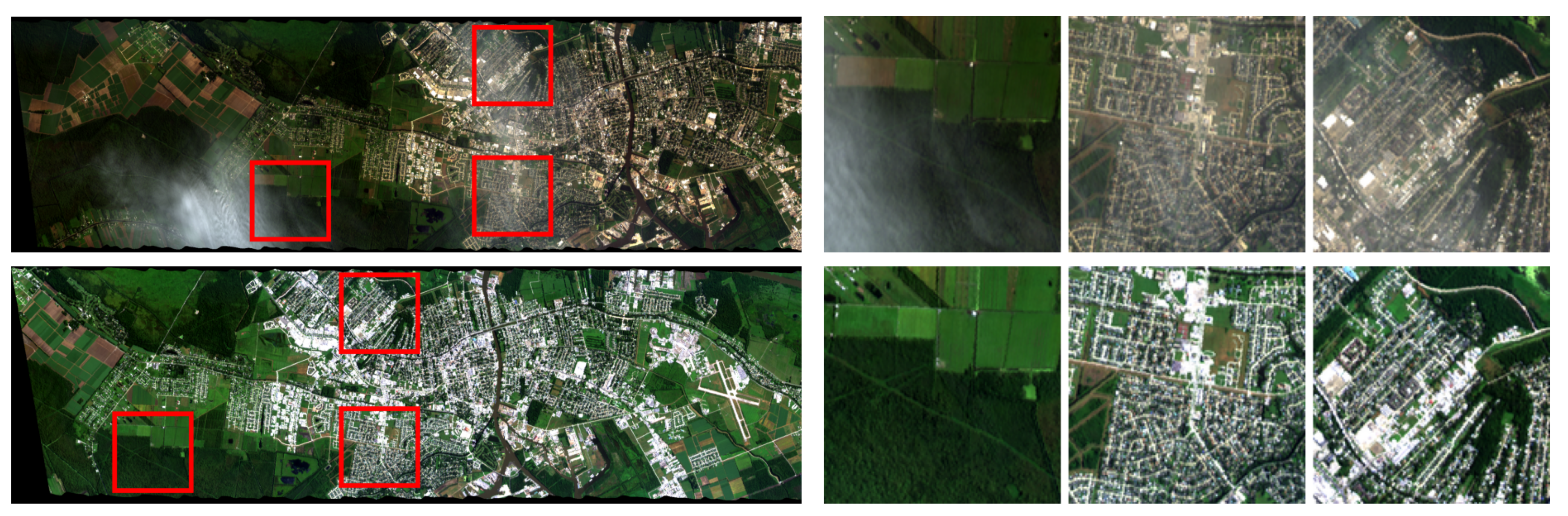
As a result, 17 distinct zones containing multiple flight-line images were identified, each including one hazy image. An example of such image pairs from the same zone is shown in Figure 4.
Each selected flight-line image underwent the following preprocessing steps:
- (1)
- DOS: ;
- (2)
-
Gain correction:, where ;
- (3)
- Normalization: pixel values were normalized using the 99.25th percentile as an upper threshold.
Haze in the selected flight-line images typically appears in localized regions rather than uniformly across the scene. Therefore, rectangular regions of pixels containing visible haze were manually annotated within each hazy flight-line image. Using these coordinates, corresponding fragments were extracted from both the hazy and haze-free flight-line images (see Figure 4).
3.1.1. Alignment
The AVIRIS data are georeferenced; however, the positional accuracy of the selected flight-line images was insufficient for precise alignment of fragments within our dataset, with errors reaching up to 10 pixels. In addition, several scenes exhibited geometric distortions that could not be corrected using standard alignment techniques (see Figure 2).
To ensure accurate registration, the following alignment procedure was employed:
- (1)
- (2)
- Fragment extraction and expert visual inspection to assess registration accuracy and identify pairs requiring additional adjustment;
- (3)
- Manual fine-tuning of transformation parameters for fragments with residual misalignment;
- (4)
- Final expert verification and exclusion of pairs where distortions could not be adequately compensated (as on Figure 2).
3.1.2. RGB Synthesis
In addition to HSI data, our dataset includes RGB version of each image generated through color synthesis from the HSI. Two color synthesis methods were applied. Color Synthesis Narrow Channels (CSNC) – based on the AVIRIS quicklook generation method, but without final JPEG compression – three narrow spectral channels are extracted: R nm, G nm, B nm. Color Synthesis Standard Observer (CSSO) [32] – based on the CIE Standard Observer color matching functions – weighted spectral integration of HS signal is performed at each pixel.
3.1.3. Subset of Pairs with Closest Scene Conditions
An additional criterion was introduced to identify the most suitable image pairs for evaluation. For full-reference metrics to accurately assess the degree of haze removal, all other imaging conditions should remain as constant as possible [33]. The primary sources of variation are illumination changes and alterations in the Earth’s surface objects (see Figure 3).
Selecting images based solely on temporal proximity is insufficient to guarantee scene similarity. As discussed in Section 2.1, certain land cover types, such as agricultural fields, may change their spectral reflectance significantly over short time intervals (see Figure 1). Therefore, expert evaluation was conducted to identify a subset of image pairs where hazy and haze-free scenes were most similar in all aspects other than the presence of haze.
3.1.4. Dataset Characteristics
The proposed dataset contains 110 hazy fragments of size pixels. Each hazy fragment is associated with at least one haze-free reference, with some having multiple references, resulting in 161 paired samples in total. Each hyperspectral image is accompanied by two RGB versions – one generated using the CSNC method and the other using CSSO.
The acquisition dates of the selected images range from August 15, 2011, to April 2, 2021, and cover diverse terrain types, including mountainous, coastal, urban, and suburban regions. Spatial resolution varies from 8 to 18 meters per pixel, depending on flight altitude.
After removing low-quality bands (104-116, 152-170, and 214-224), each image contains 182 spectral bands, spanning 365-2396 nm, consistent with established AVIRIS preprocessing practices [34].
A subset of 21 image pairs (hazy vs. clear) was identified as being most visually consistent across all parameters except for the presence of haze. Of these, 14 pairs were acquired within less than a month of each other, while 7 pairs had acquisition gaps ranging from 11 months to 1 year.
Figure 4.
A set of flight-line images consisting of one hazy and one clear image, along with three sets of extracted fragments.
Figure 4.
A set of flight-line images consisting of one hazy and one clear image, along with three sets of extracted fragments.
3.2. Field Delineation Quality Assessment
To extend the applicability of the RRealHyperPDID dataset beyond image quality assessment (IQA), its RGB subset was adapted for downstream task quality assessment (DTQA). Specifically, we evaluated the task of agricultural field delineation, which is related to segmentation but focuses on accurately detecting cultivated field boundaries relative to uncultivated land [35]. This task is essential for maintaining up-to-date cadastral maps and monitoring agricultural activities.
From the 110 scenes in RRealHyperPDID, 34 scenes containing agricultural fields were selected, corresponding to 86 clear and hazy fragments (in some cases, multiple clear fragments corresponded to a single hazy scene). In total, 3,623 fields were manually delineated by experts using CSNC RGB images.
The Delineate Anything (DA) method [36] – a state-of-the-art neural network approach – was employed for automatic delineation. The method’s pretrained model weights are publicly available, and its resolution-agnostic design allows direct application to our RGB data without additional tuning. An example of DA’s performance on clear and hazy images is shown in Figure 5: the presence of haze notably reduces delineation quality.
To quantify performance, we used both the coefficient and the object-based metric [35]. While the pixel-based metric is standard for segmentation evaluation, it is relatively insensitive to over- and under-segmentation errors, while provides a more robust assessment of delineation accuracy. A comparison of DA performance on clear and hazy fragments is presented in Table 1. As expected, delineation accuracy on hazy images is consistently lower than on haze-free ones.
3.3. RSyntHyperPDID: Remote sensing Synthetic Hyperspectral Paired Dehazing Image Dataset
We created a synthetic dataset, RSyntHyperPDID, based on the AVIRIS database. The dataset is sufficiently large to serve as a training set for dehazing models. Each RSyntHyperPDID image has a size of pixels, identical to that of RRealHyperPDID. For haze augmentation of the HSI data, we used a modified version of the CCHS method described in Section 2.1.1. Given the small fragment size and the high spatial resolution of AVIRIS, we employed a version of the method with a spatially independent parameter [23].
The proposed modification to the CCHS method concerns the generation of the HTM . Accurately extracting haze from real hazy images requires careful manual preparation: not every image contains haze, and even among those that do, extracted haze may also contain contrasting surface elements. Consequently, very few HTMs are typically used in data generation; for instance, [15] reports using only 20 distinct HTMs for the 2000 dataset images.
To overcome this limitation, instead of extracting haze from real images, we randomly generated as a two-dimensional Gaussian field with a covariance function parameterized by . This approach allows control over the spatial correlation of pixels, thereby producing diverse types of HTMs (see Figure 6). We used in our experiments.
We used 218 initial haze-free fragments, each of which was processed with two unique randomly generated HTMs. Combining this with six gamma variations, [9], resulted in 12 distinct hazed versions per fragment.
A comparison of the characteristics of the proposed datasets with other known RSID datasets is provided in Table 2.
4. Dehazing Evaluation
This section presents three experiments comparing various dehazing methods: FRIQA testing of RGB dehazing methods using RGB images from the RRealHyperPDID dataset; DTQA evaluation, assessing the influence of RGB dehazing on agricultural field delineation performance; FRIQA comparison of hyperspectral dehazing methods.
For RRealHyperPDID cases where multiple clean reference images corresponded to a single hazed image, the FRIQA metric was computed for each hazed–clean pair, and the best (maximum or minimum, depending on the metric) value was selected as the representative score for that sample.
4.1. RGB Dehazing Image Quality Assessment
We evaluated three RGB dehazing methods: DCP – the classical Dark Channel Prior method [3]; CADCP – a recent approach [7] that effectively compensates for color haze, simultaneously estimating haze density from the DCP and ambient illumination from the Color Attenuation Prior (CAP), where luminance–saturation of each pixel is linearly dependent on scene depth or haze concentration [6]; DehazeFormer – a modern neural network–based method [11] with publicly available pretrained weights.
We employed three classical metrics – PSNR, SSIM, and SAM, along with two perceptual neural metrics – LPIPS and DISTS [37]. To assess chromaticity difference, we used the specialized metric [38].
The results of the RGB dehazing methods applied to the CSNC and CSSO outputs are presented in Table 3 and Table 4, and illustrated in Figure 7. For RGB images generated with CSNC method, all dehazing methods generally improve the visual quality of hazy images, with the exception of the SAM metric, according to which only DehazeFormer achieves improvement. Among the evaluated approaches, CADCP and DehazeFormer demonstrate the best overall performance. However, while CADCP effectively removes haze, it introduces noticeable chromatic distortions, as reflected by its higher values. For RGB images generated with CSSO method, DehazeFormer achieves the highest scores for PSNR, DISTS, and LPIPS. In contrast, SSIM, SAM, and report the best values for the unprocessed (hazy) images – an inconsistency with qualitative observations. As shown in Figure 7, CADCP and DCP visibly reduce haze and, in some cases, even produce visually superior results compared to DehazeFormer.
To resolve discrepancies between quantitative metrics and perceptual quality, we conducted an expert evaluation involving four specialists from the Faculty of Space Research (Moscow State University) and the Vision Systems Laboratory (Institute for Information Transmission Problems). The experts performed pairwise comparisons among DCP, CADCP, DehazeFormer, and the original hazy images, selecting in each case the image with the least perceived haze or indicating "cannot choose". The results of the pairwise comparisons were aggregated into a global scores using the Bradley-Terry model [39]. The resulting expert-based scores are presented in Table 5. According to the expert evaluation, the methods rank in the following order of dehazing effectiveness for both RGB visualization types: CADCP; DCP; DehazeFormer; Hazed. For RGB images generated with CSNC method, this expert-derived ranking is consistent with the PSNR and DISTS metrics, while for CSSO-RGB, none of the evaluated metrics show a reliable correlation with experts’ perception.
4.1.1. Evaluation on the Subset with Closest Scenes
The discrepancy between the expert rankings and the metric-based rankings, as well as the resulting inadequacy of certain metrics, may be explained by the variation in scene content and imaging conditions, as discussed in Section 3.1.3. To clarify this issue, we compared the metric rankings separately for the subset of closely matched scenes and for the remaining scenes from the RRealHyperPDID dataset. Table 6 presents the Kendall correlation coefficients between the metric-based rankings of the dehazing algorithms and the reference expert ranking. For RGB images generated with CSNC method, the metric rankings were fully consistent with the expert ranking for the subset of closest scenes, with the only exception being the SAM metric. For the remaining scenes, the expert rankings aligned with the PSNR and DISTS metrics. For RGB images generated with CSSO method, the rankings for both subsets showed no significant correspondence with the expert evaluation.
4.2. Delineation-Based Dehazing Quality Assessment
This section presents a DTQA comparison of RGB dehazing methods based on their impact, as preprocessing steps, on the results of solving the agricultural field delineation task using the DA method [36]. The results are summarized in Table 7 and illustrated in Figure 8. All tested dehazing methods improved delineation quality, with the DehazeFormer method demonstrating the largest performance gain.
4.3. HS Dehazing Image Quality Assessment
The hyperspectral dehazing methods selected for comparison were AACNet [19], HDMba [15], and AIDTransformer [12]. Two experiments were conducted. In the first experiment, the selected neural network models were trained on the HyperDehazing dataset, following the procedures described in the corresponding publications, and subsequently tested on the RRealHyperPDID dataset, spectrally harmonized to match the spectral resolution of HyperDehazing. In the second experiment, the same models were trained on the proposed RSyntHyperPDID dataset and also evaluated on RRealHyperPDID.
The standard image quality metrics (PSNR, SSIM, and SAM) were used for evaluation. It should be noted, however, that the SAM metric showed weak correlation with expert rankings for RGB data, even within the subset of closely matched scenes. In addition, the evaluation of HS results is inherently challenging: the data cannot be assessed visually (even by experts), and the lack of field delineation methods for hyperspectral imagery makes delineation-based DTQA evaluation infeasible.
4.3.1. Experiment 1
Since pre-trained models from HyperDehazing were not publicly available, we reproduced the authors’ training procedure. As reported in [20], 1,800 images were used for training and 200 for testing; however, no exact split was provided. All models were trained for 10,000 iterations with their original hyperparameter configurations. AACNet was trained using the ADAM optimizer (, , ), batch size 32, an initial learning rate of , and a Mean Squared Error (MSE) loss function. AIDTransformer was trained using the ADAM optimizer with an initial learning rate of , cosine annealing learning rate schedule, and an loss function. HDMba was trained using the ADAM optimizer (, , ), batch size 4, an initial learning rate of a cosine annealing schedule, and a combined loss function with and . All models were implemented in the PyTorch framework and trained on NVIDIA GPUs: GeForce RTX 2080 Ti (for AACNet and AIDTransformer) and Quadro GV100 (for HDMba).
The test results on the HyperDehazing dataset achieved quality metrics comparable to those reported in [15] (Table 8). Figure 9 shows that all methods effectively removed synthetic haze, while Figure 10 presents the spectral reconstruction at a representative pixel, demonstrating that the methods approximate the clean image spectra.
The number of channels and the spectral ranges differ between HyperDehazing and RRealHyperPDID. The problem in which the response of one sensor is used to predict the response of another sensor with the known spectral sensitivity to the same radiation is called spectral harmonization [40]. We performed spectral harmonization of the RRealHyperPDID images to match the HyperDehazing configuration. Linear interpolation was used for spectral harmonization.
The metric-based results are presented in Table 9. On average, none of the HS dehazing methods produced a clear improvement over the original hazed images. This conclusion is also supported by qualitative analysis: Figure 11 shows RGB visualizations of the dehazed results, and Figure 12 presents spectral profiles at selected points.
4.3.2. Experiment 2
The RSyntHyperPDID dataset was divided into training and validation subsets containing 2,354 and 262 fragments, respectively. The training hyperparameters were identical to those used for the HyperDehazing dataset, see the previous section.
The quantitative results for the RSyntHyperPDID test set and the real-haze RRealHyperPDID dataset are presented in Table 10. Both the metric evaluations and the qualitative analysis (see Figure 13) demonstrate that models trained on RSyntHyperPDID effectively remove haze from real hazy images. This conclusion is further supported by the spectral decomposition results (Figure 14).
5. Conclusions
This work presents a comprehensive benchmark for hyperspectral remote sensing image dehazing (RSID) that integrates real and synthetic data, standardized evaluation protocols, and baseline implementations of state-of-the-art algorithms. The proposed benchmark includes data splits from the well-known HyperDehazing dataset, the proposed real-world test set (RRealHyperPDID) with paired hazy and haze-free hyperspectral images, and the proposed synthetic training set (RSyntHyperPDID) generated using the CCHS haze simulation method. In addition, we provide an open-source evaluation suite that combines image quality and delineation-based metrics, establishing a unified framework for the assessment of dehazing performance in hyperspectral remote sensing.
The conducted experiments reveal several important insights. RGB-based RSID methods are capable of effectively compensating for real haze in remote sensing imagery. The neural network–based DehazeFormer, trained on synthetic data, demonstrates competitive performance, although classical model-driven approaches such as DCP and CADCP may still achieve superior results. The reliability of image quality metrics was found to depend strongly on the acquisition setup: for CSSO imagery, common universal metrics such as PSNR, SSIM, SAM, DISTS, and LPIPS showed poor correlation with expert evaluations, whereas for CSNC data, PSNR, SSIM, LPIPS, and DISTS aligned well with expert judgment. Notably, PSNR and DISTS remained consistent even in complex scenes where haze was not the sole source of degradation.
The results also demonstrate the practical significance of dehazing as a preprocessing step. When applied before agricultural field delineation, DehazeFormer improved delineation accuracy across all types of RGB imagery, with little dependence on the specific imaging configuration. However, experiments with hyperspectral data revealed a clear domain gap: models trained solely on the synthetic HyperDehazing dataset failed to generalize to real haze conditions, even after spectral harmonization designed to mitigate channel mismatches.
By contrast, HS dehazing models trained on the proposed RSyntHyperPDID dataset successfully remove real haze, indicating that RSyntHyperPDID provides a more representative and transferable basis for model training. Among the evaluated architectures, AIDTransformer achieved the highest PSNR and the most stable reconstruction performance.
Overall, the proposed benchmark provides a robust and reproducible foundation for advancing research in hyperspectral dehazing.
Author Contributions
Conceptualization, A.N. and D.N.; methodology, D.S. and D.N.; formal analysis N.O.; software, N.O., V.V. and E.D.; validation, A.N., D.S. and D.N.; investigation, A.N., D.S., N.O., A.S., E.D. and M.Z.; resources, N.O. data curation, N.O., E.D. and M.Z.; writing—original draft preparation, D.S.; writing—review and editing, A.S.; visualization, N.O., V.V., E.D., M.Z.; supervision, A.N. and D.N.; project administration, D.S.; funding acquisition, A.N. All authors have read and agreed to the published version of the manuscript.
Funding
This work was supported by the Ministry of Economic Development of the Russian Federation (agreement identifier 000000C313925P3U0002, grant No 139-15-2025-003 dated 16.04.2025).
Data Availability Statement
The proposed datasets are publicly available at https://huggingface.co/datasets/nikos74/RRealHyperPDID for RRealHyperPDID and https://huggingface.co/datasets/nikos74/RSyntHyperPDID for RSyntHyperPDID. Additional datasets analyzed in this study are available at: HyperDehazing dataset at https://github.com/RsAI-lab/HyperDehazing (accessed on 10 October 2025) and RRSHID dataset at https://huggingface.co/datasets/lwCVer/RRSHID (accessed on 10 October 2025). All source code, including neural network architectures, preprocessing scripts, training routines, and evaluation tools, is openly available at: https://github.com/iitpvisionlab/hyperhazeoff.
Acknowledgments
We thank Vyacheslav Volosyankin for his valuable assistance in conducting the expert evaluations.
Conflicts of Interest
The authors declare no conflicts of interest.
Abbreviations
The following abbreviations are used in this manuscript:
| RRealHyperPDID | Remote sensing Real-world Hyperspectral Paired Dehazing Image Dataset |
| RSyntHyperPDID | Remote Sensing Synthetic Hyperspectral Paired Dehazing Image Dataset |
| HSI | Hyperspectral image |
| CNN | Convolutional neural network |
| RSID | Remote sensing image dehazing |
| RRSHID | Real-World Remote Sensing Hazy Image Dataset |
| DTQA | Downstream Task Quality Assessment |
| IQA | Image quality assessment |
| AS | Atmospheric Scattering |
| HTM | Haze transmission map |
| DOS | Dark-Object Subtraction |
| HHS | Hazy HSI Synthesis |
| CCHS | Channel Correlation based Haze Synthesis |
| FRIQA | Full Reference IQA |
| NRIQA | No Reference IQA |
| RMSE | Root Mean Square Error |
| PSNR | Peak Signal-to-Noise Ratio |
| SSIM | Structural Similarity Index |
| SAM | Spectral Angle Mapper |
| LPIPS | Learned Perceptual Image Patch Similarity |
| NDVI | Normalized Difference Vegetation Index |
| SIFT | Scale-Invariant Feature Transform |
| RANSAC | RANdom SAmple Consensus |
| CSNC | Color Synthesis Narrow Channels |
| CSSO | Color Synthesis Standard Observer |
| DA | Delineate Anything |
| DCP | Dark Channel Prior |
| CADCP | Color Attenuation Dark Channel Prior |
| CAP | Color Attenuation Prior |
| MSE | Mean Squared Error |
References
- Li, C.; Li, Z.; Liu, X.; Li, S. The influence of image degradation on hyperspectral image classification. Remote Sensing 2022, 14, 5199. [Google Scholar] [CrossRef]
- Kokhan, V.L.; Konyushenko, I.D.; Bocharov, D.A.; Seleznev, I.O.; Nikolaev, I.P.; Nikolaev, D.P. TSQ-2024: A Categorized Dataset of 2D LiDAR Images of Moving Dump Trucks in Various Environment Conditions. In Proceedings of the ICMV 2024; Osten, W.; Nikolaev, D.; Debayle, J., Eds., Bellingham, 2025; Vol. 13517, Washington 98227-0010 USA; pp. 1351709–6. [Google Scholar] [CrossRef]
- He, K.; Sun, J.; Tang, X. Single image haze removal using dark channel prior. IEEE transactions on pattern analysis and machine intelligence 2010, 33, 2341–2353. [Google Scholar]
- Long, J.; Shi, Z.; Tang, W.; Zhang, C. Single remote sensing image dehazing. IEEE Geoscience and Remote Sensing Letters 2013, 11, 59–63. [Google Scholar] [CrossRef]
- Ju, M.; Ding, C.; Guo, Y.J.; Zhang, D. Remote sensing image haze removal using gamma-correction-based dehazing model. IEEE Access 2018, 7, 5250–5261. [Google Scholar] [CrossRef]
- Zhu, Z.; Luo, Y.; Wei, H.; Li, Y.; Qi, G.; Mazur, N.; Li, Y.; Li, P. Atmospheric light estimation based remote sensing image dehazing. Remote Sensing 2021, 13, 2432. [Google Scholar] [CrossRef]
- Sidorchuk, D.S.; Pavlova, M.A.; Kushchev, D.O.; Selyugin, M.A.; Nikolaev, I.P.; Bocharov, D.A. CADCP: a method for chromatic haze compensation on remotely sensed images. In Proceedings of the ICMV 2023; Osten, W.; Nikolaev, D.; Debayle, J., Eds., Bellingham, Apr. 2024; Vol. 13072, Washington 98227-0010 USA; pp. 1307216–10. [Google Scholar] [CrossRef]
- Qin, X.; Wang, Z.; Bai, Y.; Xie, X.; Jia, H. dehazing. In Proceedings of the Proceedings of the AAAI conference on artificial intelligence, 2020, Vol.
- Guo, J.; Yang, J.; Yue, H.; Tan, H.; Hou, C.; Li, K. RSDehazeNet: Dehazing network with channel refinement for multispectral remote sensing images. IEEE Transactions on geoscience and remote sensing 2020, 59, 2535–2549. [Google Scholar] [CrossRef]
- Wen, X.; Pan, Z.; Hu, Y.; Liu, J. An effective network integrating residual learning and channel attention mechanism for thin cloud removal. IEEE Geoscience and Remote Sensing Letters 2022, 19, 1–5. [Google Scholar] [CrossRef]
- Song, Y.; He, Z.; Qian, H.; Du, X. Vision transformers for single image dehazing. IEEE Transactions on Image Processing 2023, 32, 1927–1941. [Google Scholar] [CrossRef]
- Kulkarni, A.; Murala, S. Aerial image dehazing with attentive deformable transformers. In Proceedings of the Proceedings of the IEEE/CVF winter conference on applications of computer vision, 2023, pp.
- Song, T.; Fan, S.; Li, P.; Jin, J.; Jin, G.; Fan, L. Learning an effective transformer for remote sensing satellite image dehazing. IEEE Geoscience and Remote Sensing Letters 2023, 20, 1–5. [Google Scholar] [CrossRef]
- Zhou, H.; Wu, X.; Chen, H.; Chen, X.; He, X. Rsdehamba: Lightweight vision mamba for remote sensing satellite image dehazing. arXiv preprint arXiv:2405.10030, arXiv:2405.10030 2024.
- Fu, H.; Sun, G.; Li, Y.; Ren, J.; Zhang, A.; Jing, C.; Ghamisi, P. HDMba: hyperspectral remote sensing imagery dehazing with state space model. arXiv preprint arXiv:2406.05700, arXiv:2406.05700 2024.
- Ancuti, C.O.; Ancuti, C.; Timofte, R.; De Vleeschouwer, C. images. In Proceedings of the Proceedings of the IEEE conference on computer vision and pattern recognition workshops, 2018, pp.
- Feng, Y.; Su, Z.; Ma, L.; Li, X.; Liu, R.; Zhou, F. Bridging the Gap Between Haze Scenarios: A Unified Image Dehazing Model. IEEE Transactions on Circuits and Systems for Video Technology 2024. [Google Scholar] [CrossRef]
- Zhu, Z.H.; Lu, W.; Chen, S.B.; Ding, C.H.; Tang, J.; Luo, B. Real-World Remote Sensing Image Dehazing: Benchmark and Baseline. IEEE Transactions on Geoscience and Remote Sensing 2025. [Google Scholar] [CrossRef]
- Xu, M.; Peng, Y.; Zhang, Y.; Jia, X.; Jia, S. AACNet: Asymmetric attention convolution network for hyperspectral image dehazing. IEEE Transactions on Geoscience and Remote Sensing 2023, 61, 1–14. [Google Scholar] [CrossRef]
- Fu, H.; Ling, Z.; Sun, G.; Ren, J.; Zhang, A.; Zhang, L.; Jia, X. HyperDehazing: A hyperspectral image dehazing benchmark dataset and a deep learning model for haze removal. ISPRS Journal of Photogrammetry and Remote Sensing 2024, 218, 663–677. [Google Scholar] [CrossRef]
- Pan, X.; Xie, F.; Jiang, Z.; Yin, J. Haze removal for a single remote sensing image based on deformed haze imaging model. IEEE Signal Processing Letters 2015, 22, 1806–1810. [Google Scholar] [CrossRef]
- Kang, X.; Fei, Z.; Duan, P.; Li, S. Fog model-based hyperspectral image defogging. IEEE Transactions on Geoscience and Remote Sensing 2021, 60, 1–12. [Google Scholar] [CrossRef]
- Qin, M.; Xie, F.; Li, W.; Shi, Z.; Zhang, H. Dehazing for multispectral remote sensing images based on a convolutional neural network with the residual architecture. IEEE journal of selected topics in applied earth observations and remote sensing 2018, 11, 1645–1655. [Google Scholar] [CrossRef]
- Wang, Z.; Bovik, A.C.; Sheikh, H.R.; Simoncelli, E.P. Image quality assessment: from error visibility to structural similarity. IEEE transactions on image processing 2004, 13, 600–612. [Google Scholar] [CrossRef]
- Kruse, F.A.; Lefkoff, A.B.; Boardman, J.W.; Heidebrecht, K.B.; Shapiro, A.; Barloon, P.; Goetz, A.F. The spectral image processing system (SIPS)—interactive visualization and analysis of imaging spectrometer data. Remote sensing of environment 1993, 44, 145–163. [Google Scholar] [CrossRef]
- Zhang, R.; Isola, P.; Efros, A.A.; Shechtman, E.; Wang, O. The unreasonable effectiveness of deep features as a perceptual metric. In Proceedings of the Proceedings of the IEEE conference on computer vision and pattern recognition, 2018, pp.
- Choi, L.K.; You, J.; Bovik, A.C. Referenceless prediction of perceptual fog density and perceptual image defogging. IEEE Transactions on Image Processing 2015, 24, 3888–3901. [Google Scholar] [CrossRef] [PubMed]
- Gu, K.; Tao, D.; Qiao, J.F.; Lin, W. Learning a no-reference quality assessment model of enhanced images with big data. IEEE transactions on neural networks and learning systems 2017, 29, 1301–1313. [Google Scholar] [CrossRef] [PubMed]
- Guan, T.; Li, C.; Gu, K.; Liu, H.; Zheng, Y.; Wu, X.j. Visibility and distortion measurement for no-reference dehazed image quality assessment via complex contourlet transform. IEEE Transactions on Multimedia 2022, 25, 3934–3949. [Google Scholar] [CrossRef]
- Lowe, D.G. Object recognition from local scale-invariant features. In Proceedings of the Proceedings of the seventh IEEE international conference on computer vision.
- Fischler, M.A.; Bolles, R.C. Random sample consensus: a paradigm for model fitting with applications to image analysis and automated cartography. Communications of the ACM 1981, 24, 381–395. [Google Scholar] [CrossRef]
- Magnusson, M.; Sigurdsson, J.; Armansson, S.E.; Ulfarsson, M.O.; Deborah, H.; Sveinsson, J.R. Creating RGB images from hyperspectral images using a color matching function. In Proceedings of the IGARSS 2020-2020 IEEE International Geoscience and Remote Sensing Symposium. IEEE; 2020; pp. 2045–2048. [Google Scholar]
- Pavlova, M.A.; Sidorchuk, D.S.; Kushchev, D.O.; Bocharov, D.A.; Nikolaev, D.P. Equalization of Shooting Conditions Based on Spectral Models for the Needs of Precision Agriculture Using UAVs. JCTE 2022, 67. [Google Scholar] [CrossRef]
- Tang, P.W.; Lin, C.H. Hyperspectral Dehazing Using Admm-Adam Theory. In Proceedings of the 2022 12th Workshop on Hyperspectral Imaging and Signal Processing: Evolution in Remote Sensing (WHISPERS); 2022; pp. 1–5. [Google Scholar] [CrossRef]
- Pavlova, M.A.; Timofeev, V.A.; Bocharov, D.A.; Sidorchuk, D.S.; Nurmukhametov, A.L.; Nikonorov, A.V.; Yarykina, M.S.; Kunina, I.A.; Smagina, A.A.; Zagarev, M.A. Low-parameter method for delineation of agricultural fields in satellite images based on multi-temporal MSAVI2 data. Computer Optics 2023, 47, 451–463. [Google Scholar] [CrossRef]
- Lavreniuk, M.; Kussul, N.; Shelestov, A.; Yailymov, B.; Salii, Y.; Kuzin, V.; Szantoi, Z. Delineate Anything: Resolution-Agnostic Field Boundary Delineation on Satellite Imagery. arXiv preprint arXiv:2504.02534, arXiv:2504.02534 2025.
- Ding, K.; Ma, K.; Wang, S.; Simoncelli, E.P. Image quality assessment: Unifying structure and texture similarity. IEEE transactions on pattern analysis and machine intelligence 2020, 44, 2567–2581. [Google Scholar] [CrossRef]
- Sidorchuk, D.S.; Nurmukhametov, A.L.; Maximov, P.V.; Bozhkova, V.P.; Sarycheva, A.P.; Pavlova, M.A.; Kazakova, A.A.; Gracheva, M.A.; Nikolaev, D.P. Leveraging Achromatic Component for Trichromat-Friendly Daltonization. J. Imaging 2025, 11, 1–24. [Google Scholar] [CrossRef] [PubMed]
- Li, S.; Ma, H.; Hu, X. Neural image beauty predictor based on bradley-terry model. arXiv preprint arXiv:2111.10127, arXiv:2111.10127 2021.
- Nurmukhametov, A.; Sidorchuk, D.; Skidanov, R. Harmonization of hyperspectral and multispectral data for calculation of vegetation index. Journal of Communications Technology and Electronics 2024, 69, 38–45. [Google Scholar] [CrossRef]
Figure 1.
Examples from RRSHID [18] showing scenes with significant temporal changes between paired hazy and haze-free images.
Figure 1.
Examples from RRSHID [18] showing scenes with significant temporal changes between paired hazy and haze-free images.
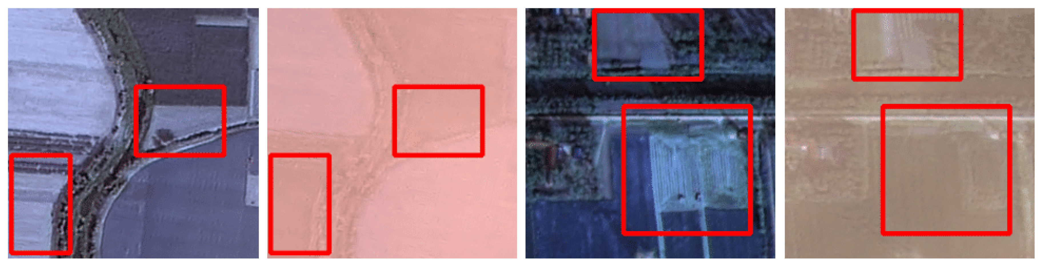
Figure 2.
An example of complex geometric distortions in AVIRIS data.
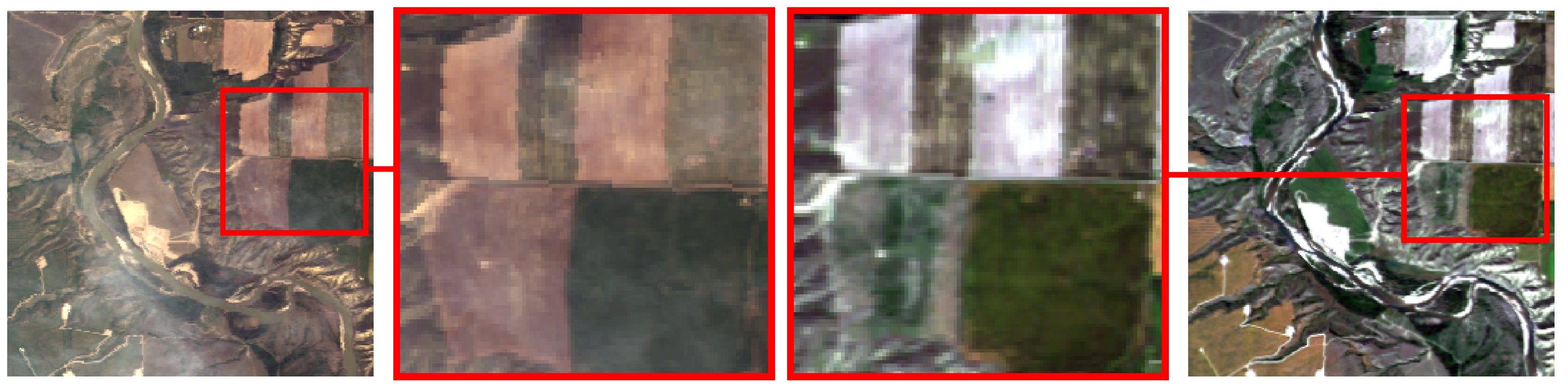
Figure 3.
Examples of images from RRealHyperPDID showing the same area of the surface that has changed significantly between acquisitions acquired just 19 days apart, 18.04.2014 and 07.05.2014
Figure 3.
Examples of images from RRealHyperPDID showing the same area of the surface that has changed significantly between acquisitions acquired just 19 days apart, 18.04.2014 and 07.05.2014
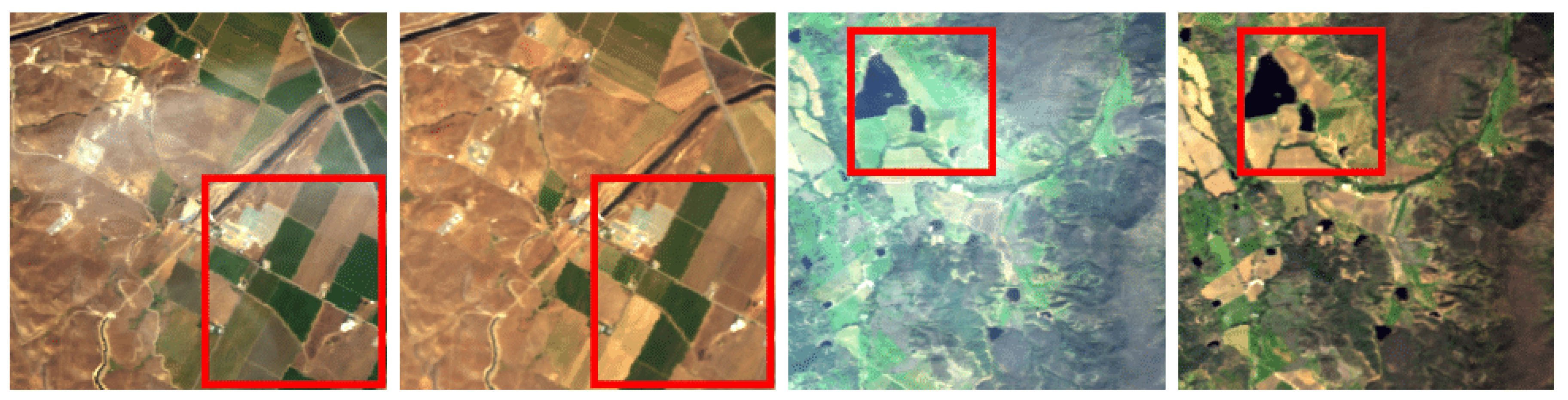
Figure 5.
Results of applying the agricultural field delineation method DA to clean and hazy RGB images from RRealHyperPDID dataset.
Figure 5.
Results of applying the agricultural field delineation method DA to clean and hazy RGB images from RRealHyperPDID dataset.
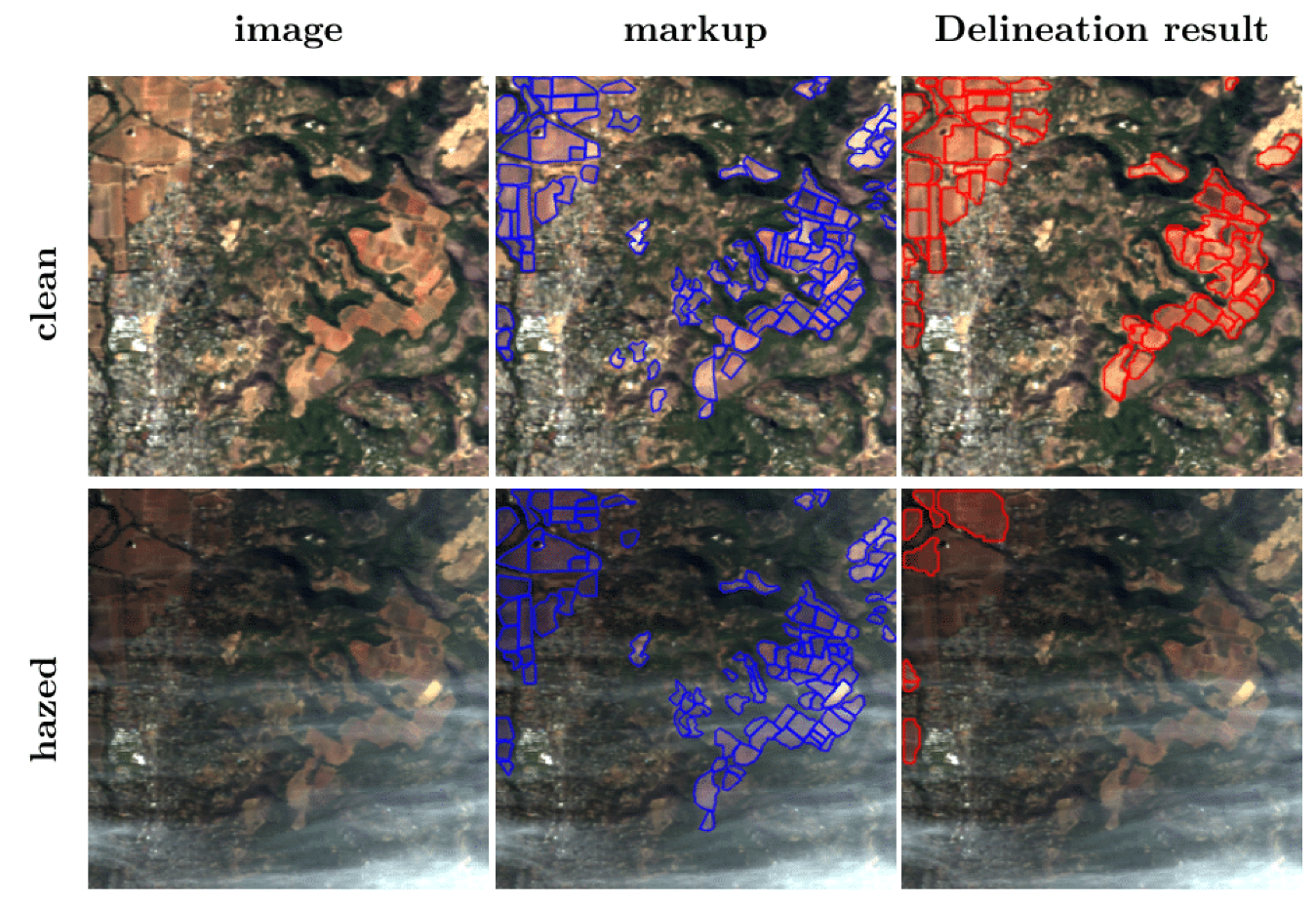
Figure 6.
Examples of randomly generated maps with parameters .
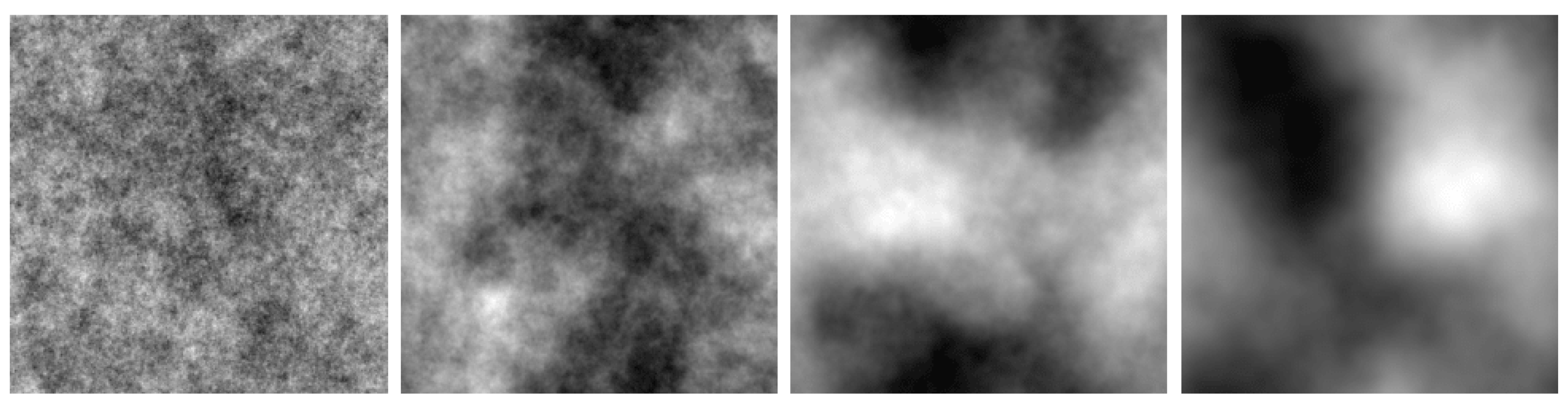
Figure 7.
Examples of RGB dehazing results.
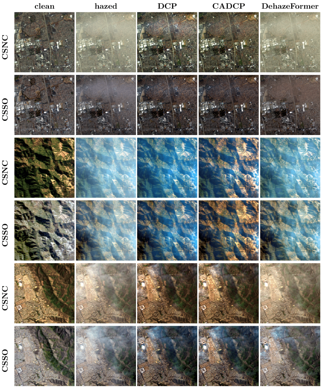
Figure 8.
Results of applying the DA algorithm to hazed and dehazed images.
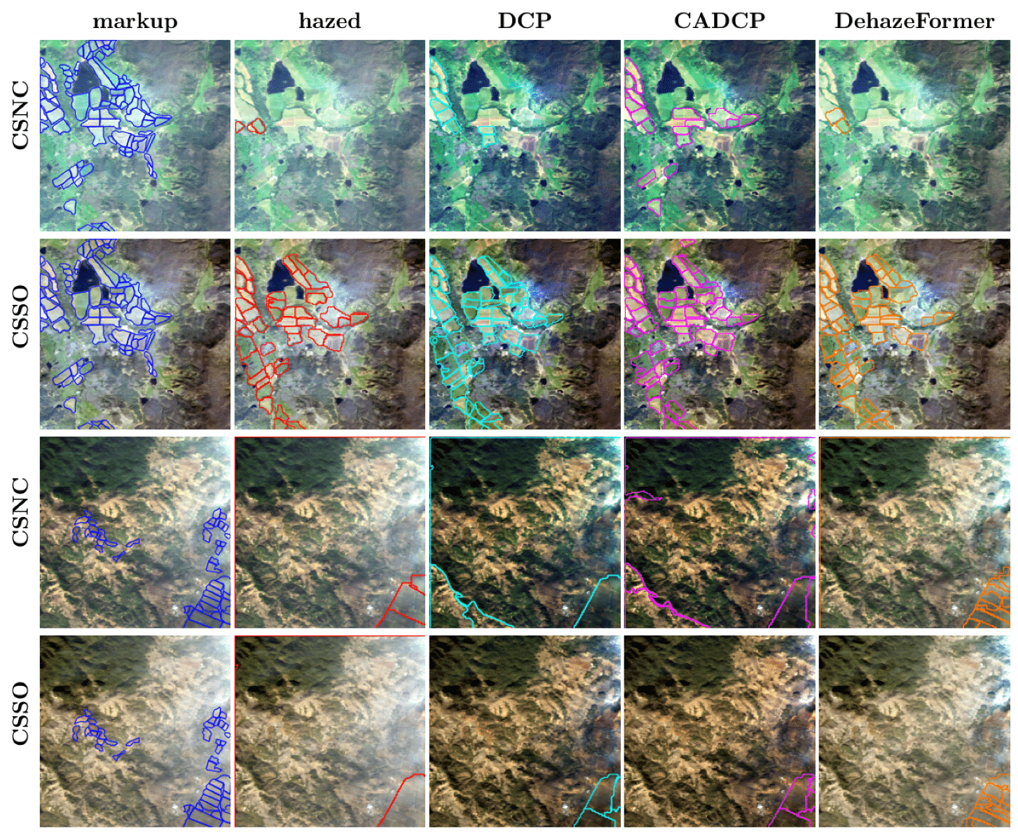
Figure 9.
RGB visualization comparison of hyperspectral dehazing methods trained on the HyperDehazing synthetic training set and evaluated on the test set.
Figure 9.
RGB visualization comparison of hyperspectral dehazing methods trained on the HyperDehazing synthetic training set and evaluated on the test set.
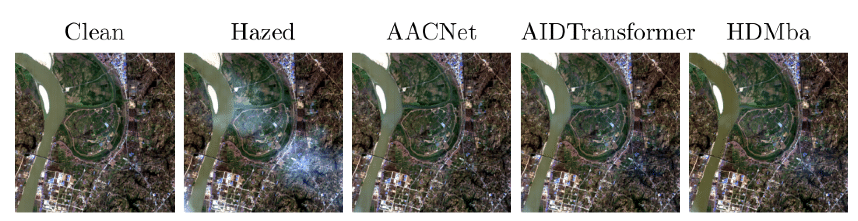
Figure 10.
Spectral reconstruction performance for various HS dehazing methods on the HyperDehazing test set.
Figure 10.
Spectral reconstruction performance for various HS dehazing methods on the HyperDehazing test set.
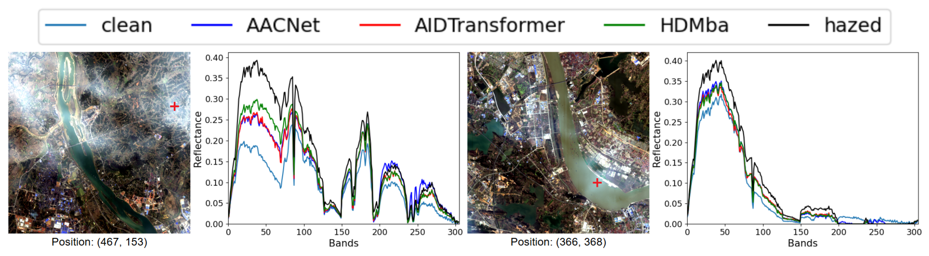
Figure 11.
RGB visualization comparison of hyperspectral dehazing methods trained on the HyperDehazing synthetic dataset and tested on the RRealHyperPDID real-world dataset.
Figure 11.
RGB visualization comparison of hyperspectral dehazing methods trained on the HyperDehazing synthetic dataset and tested on the RRealHyperPDID real-world dataset.
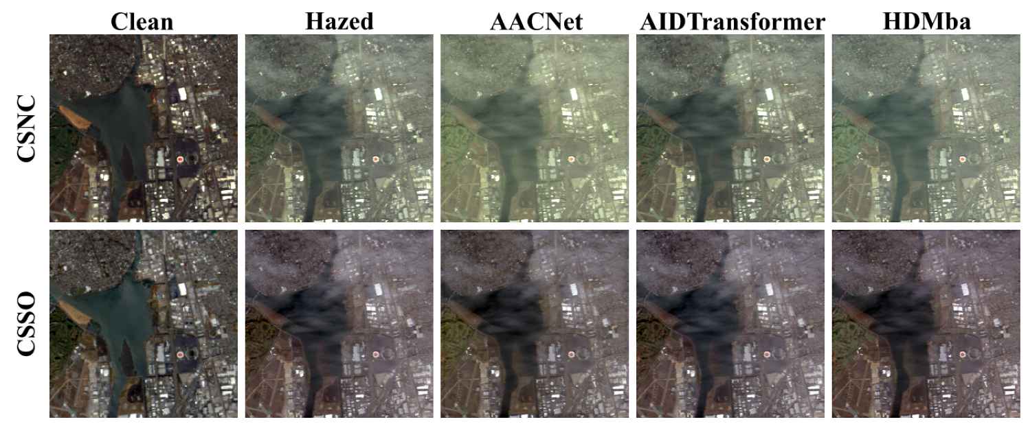
Figure 12.
Spectral reconstruction performance for HS dehazing methods on the RRealHyperPDID test set.
Figure 12.
Spectral reconstruction performance for HS dehazing methods on the RRealHyperPDID test set.
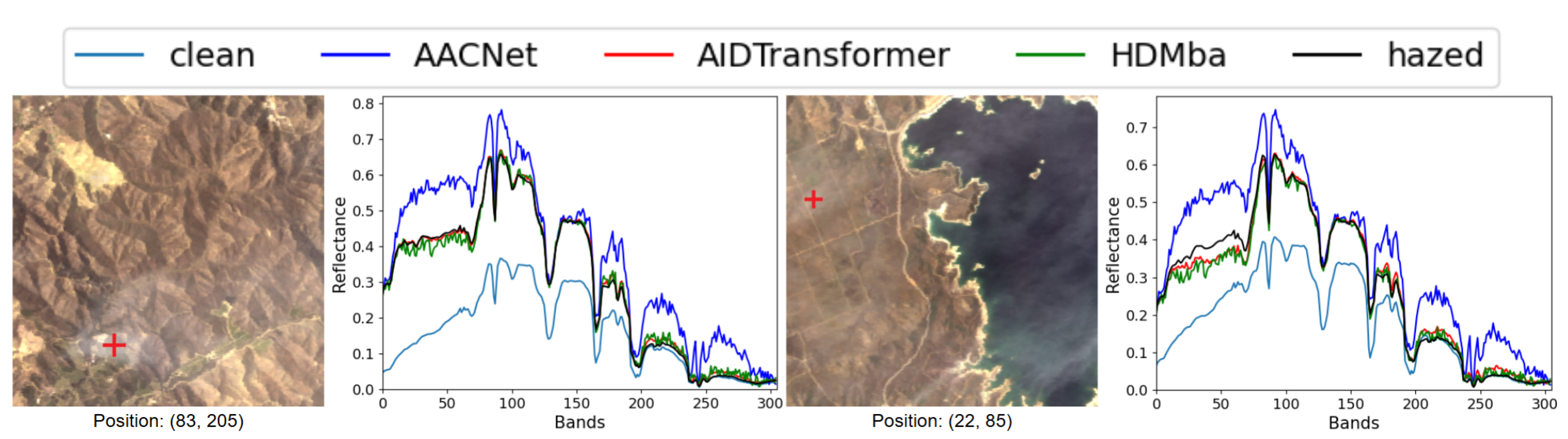
Figure 13.
RGB visualization comparison of hyperspectral dehazing methods trained on the RSyntHyperPDID synthetic dataset and tested on the RRealHyperPDID real-world dataset.
Figure 13.
RGB visualization comparison of hyperspectral dehazing methods trained on the RSyntHyperPDID synthetic dataset and tested on the RRealHyperPDID real-world dataset.
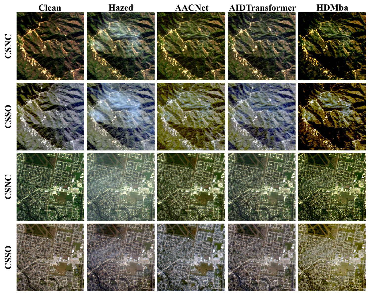
Figure 14.
Spectral reconstruction performance for HS dehazing methods trained on RSyntHyperPDID.
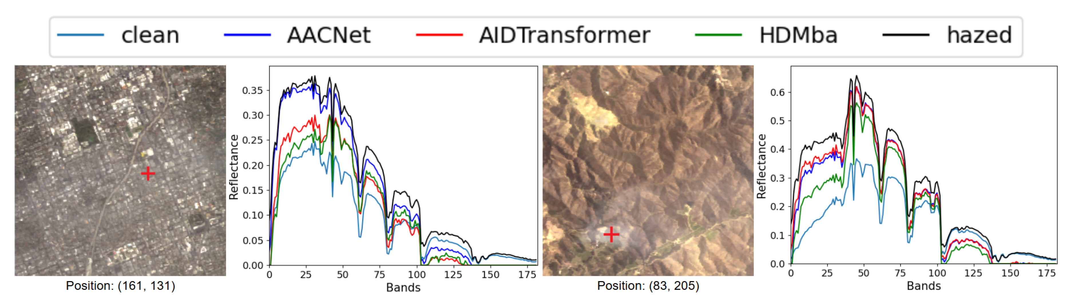

Table 1.
Comparison of the agricultural field delineation method DA results for clean and hazy RGB images.
Table 1.
Comparison of the agricultural field delineation method DA results for clean and hazy RGB images.
| Data | DICE | number of images | |
|---|---|---|---|
| clean (CSNC) | 58.17 | 24.41 | 52 |
| hazed (CSNC) | 38.59 | 15.93 | 34 |
| clean (CSSO) | 50.59 | 23.26 | 52 |
| hazed (CSSO) | 42.61 | 20.93 | 34 |
Table 2.
Comparison of the proposed datasets, RRealHyperPDID and RSyntHyperPDID, with existing remote sensing dehazing datasets.
Table 2.
Comparison of the proposed datasets, RRealHyperPDID and RSyntHyperPDID, with existing remote sensing dehazing datasets.
| Dataset | Size | Real/ Synthetic | Paired | Resolution | Image Type |
|---|---|---|---|---|---|
| RRSHID [18] | 3,053 | Real | Yes | 256×256 | RGB |
| RS-Haze [11] | 51,300 | Synthetic | Yes | 512×512 | RGB |
| HyperDehazing [20] | 2,000 | Synthetic | Yes | 512×512 | Hyperspectral |
| HyperDehazing [20] | 70 | Real | No | 512×512 | Hyperspectral |
| HDD [22] | 40 | Real | No | 512×512 | Hyperspectral |
| RRealHyperPDID | 110 | Real | Yes | 256×256 | Hyperspectral |
| RSyntHyperPDID | 2,616 | Synthetic | Yes | 256×256 | Hyperspectral |
Table 3.
Results of various RGB dehazing methods on RGB images (CSNC RGB generation method) of RRealHyperPDID images.
Table 3.
Results of various RGB dehazing methods on RGB images (CSNC RGB generation method) of RRealHyperPDID images.
| Method | PSNR↑ | SSIM↑ | SAM↓ | DIST↓ | LPIPS↓ | |
|---|---|---|---|---|---|---|
| No dehazing | 13.81 | 0.555 | 0.197 | 0.242 | 0.401 | 0.170 |
| DCP [3] | 16.08 | 0.570 | 0.242 | 0.219 | 0.398 | 0.170 |
| CADCP [7] | 16.26 | 0.575 | 0.228 | 0.214 | 0.391 | 0.186 |
| DehazeFormer [11] | 15.07 | 0.575 | 0.185 | 0.222 | 0.390 | 0.157 |
Table 4.
Results of various RGB dehazing methods on (CSSO RGB generation method) of RRealHyperPDID images.
Table 4.
Results of various RGB dehazing methods on (CSSO RGB generation method) of RRealHyperPDID images.
| Method | PSNR↑ | SSIM↑ | SAM↓ | DIST↓ | LPIPS↓ | |
|---|---|---|---|---|---|---|
| No dehazing | 16.06 | 0.598 | 0.159 | 0.227 | 0.415 | 0.143 |
| DCP [3] | 14.95 | 0.546 | 0.231 | 0.227 | 0.420 | 0.193 |
| CADCP [7] | 15.00 | 0.548 | 0.228 | 0.226 | 0.419 | 0.191 |
| DehazeFormer [11] | 16.75 | 0.597 | 0.171 | 0.211 | 0.404 | 0.151 |
Table 5.
Expert comparison of RGB dehazing methods on RRealHyperPDID.
| Method | CSNC | CSSO |
|---|---|---|
| No dehazing | 0.0005 | 0.0007 |
| DCP | 0.3068 | 0.3558 |
| CADCP | 0.6762 | 0.6027 |
| DehazeFormer | 0.0165 | 0.0408 |
Table 6.
Kendall correlation coefficients between metric-based and expert rankings of dehazing algorithms.
Table 6.
Kendall correlation coefficients between metric-based and expert rankings of dehazing algorithms.
| Close scenes | Other scenes | |||||||||
|---|---|---|---|---|---|---|---|---|---|---|
| PSNR | SSIM | SAM | DISTS | LPIPS | PSNR | SSIM | SAM | DISTS | LPIPS | |
| CSNC | ||||||||||
| 1 | 1 | 0.3 | 1 | 1 | 1 | 0.3 | -0.3 | 1 | 0 | |
| CSSO | ||||||||||
| -0.55 | -0.55 | -0.91 | 0.18 | 0.18 | -0.33 | -0.67 | -0.67 | -0.33 | -0.33 | |
Table 7.
Comparison of DA results for hazed and dehazed images processed with DCP, CADCP, and DehazeFormer algorithms.
Table 7.
Comparison of DA results for hazed and dehazed images processed with DCP, CADCP, and DehazeFormer algorithms.
| CSNC | CSSO | |||
|---|---|---|---|---|
| Data | ||||
| hazed | 38.59 | 15.93 | 42.61 | 20.93 |
| DCP [3] | 43.16 | 18.01 | 47.22 | 22.88 |
| CADCP [7] | 45.95 | 19.36 | 47.35 | 21.45 |
| DehazeFormer [11] | 46.92 | 20.55 | 50.31 | 23.22 |
| clean | 58.17 | 24.41 | 50.59 | 23.26 |
Table 8.
Reproduction of neural network HSI dehazing results on the HyperDehazing test set. Results for hazed images were not provided in [15].
Table 8.
Reproduction of neural network HSI dehazing results on the HyperDehazing test set. Results for hazed images were not provided in [15].
| Our results | [15] results | ||||||
|---|---|---|---|---|---|---|---|
| Method | PSNR↑ | SSIM↑ | SAM↓ | PSNR↑ | SSIM↑ | SAM↓ | |
| No dehazing | 32.81 | 0.9513 | 0.0348 | - | - | - | |
| AACNet [19] | 40.44 | 0.9572 | 0.0189 | 37.43 | 0.9734 | 0.0425 | |
| AIDTransformer [12] | 38.13 | 0.9553 | 0.0262 | 35.47 | 0.9723 | 0.0401 | |
| HDMba [15] | 36.16 | 0.9525 | 0.0352 | 38.13 | 0.9763 | 0.0382 | |
Table 9.
Results of HS dehazing methods on RRealHyperPDID. Models trained on HyperDehazing training set.
Table 9.
Results of HS dehazing methods on RRealHyperPDID. Models trained on HyperDehazing training set.
| Method | PSNR↑ | SSIM↑ | SAM↓ |
|---|---|---|---|
| No dehazing | 34.68 | 0.638 | 0.210 |
| AACNet [19] | 16.07 | 0.228 | 0.368 |
| AIDTransformer [12] | 18.40 | 0.346 | 0.216 |
| HDMba [15] | 16.44 | 0.266 | 0.288 |
Table 10.
Results of neural network-based HS dehazing methods on the validation subset of the synthetic-haze RSyntHyperPDID and real-haze RRealHyperPDID. Models trained on RSyntHyperPDID training set.
Table 10.
Results of neural network-based HS dehazing methods on the validation subset of the synthetic-haze RSyntHyperPDID and real-haze RRealHyperPDID. Models trained on RSyntHyperPDID training set.
| RSyntHyperPDID test | RRealHyperPDID | ||||||
|---|---|---|---|---|---|---|---|
| Method | PSNR↑ | SSIM↑ | SAM↓ | PSNR↑ | SSIM↑ | SAM↓ | |
| No dehazing | 23.54 | 0.9193 | 0.1271 | 25.28 | 0.6765 | 0.2293 | |
| AACNet [19] | 33.06 | 0.9683 | 0.0533 | 26.62 | 0.6514 | 0.2092 | |
| AIDTransformer [12] | 31.42 | 0.9554 | 0.0620 | 26.88 | 0.5929 | 0.2460 | |
| HDMba [15] | 28.54 | 0.9411 | 0.0840 | 26.78 | 0.5517 | 0.2731 | |
Disclaimer/Publisher’s Note: The statements, opinions and data contained in all publications are solely those of the individual author(s) and contributor(s) and not of MDPI and/or the editor(s). MDPI and/or the editor(s) disclaim responsibility for any injury to people or property resulting from any ideas, methods, instructions or products referred to in the content. |
© 2025 by the authors. Licensee MDPI, Basel, Switzerland. This article is an open access article distributed under the terms and conditions of the Creative Commons Attribution (CC BY) license (http://creativecommons.org/licenses/by/4.0/).
Copyright: This open access article is published under a Creative Commons CC BY 4.0 license, which permit the free download, distribution, and reuse, provided that the author and preprint are cited in any reuse.


