
Submitted:
23 January 2024
Posted:
24 January 2024
You are already at the latest version
Abstract
With the development of artificial intelligence, the ability of capturing the background characteristics of hyperspectral imagery (HSI) is improved and promising performance in hyperspectral anomaly detection (HAD) tasks is yielded. However, existing methods proposed in recent years still suffer from certain limitations: 1) constraints are lacking in the deep feature learning process in terms of the issue for absence of prior background and anomaly information. 2) hyperspectral anomaly detectors with traditional self-supervised deep learning methods fail to ensure prioritized reconstruction of the background. 3) architectures of fully connected deep network in hyperspectral anomaly detectors lead to low utilization of spatial information and destruction for original spatial relationship of hyperspectral imagery, and disregard spectral correlation between adjacent pixels. 4) hypotheses or assumptions for background and anomaly distributions restrict the performance of many hyperspectral anomaly detectors because the distributions of background land covers are usually complex and not assumable in real-world hyperspectral imagery. With the consideration of above problems, in this paper, we propose a novel fully convolutional auto-encoder based on dual clustering and latent feature adversarial consistency (FCAE-DCAC) for HAD which is carried out in a self-supervised learning-based processing. Firstly, the density-based spatial clustering of applications with noise algorithm and connected component analysis are utilized for successive spectral and spatial clustering to obtain more precise prior background and anomaly information, which facilitates the separation between background and anomaly samples during the training of our method. Subsequently, a novel fully convolutional auto-encoder (FCAE) integrated with spatial-spectral joint attention (SSJA) is proposed to enhance the utilization of spatial information and augment feature expression. In addition, a latent feature adversarial consistency network is proposed to achieve pure background reconstruction with the ability of learning actual background distribution in hyperspectral imagery. Finally, a triplet loss is introduced to enhance the separability between background and anomaly, and the reconstruction residual serves as the anomaly detection result. We evaluate the proposed method on seven groups of real-world hyperspectral datasets, and the experimental results confirmed the effectiveness and superior performance of the proposed method versus nine state-of-the-art methods.
Keywords:
hyperspectral imagery
; anomaly detection
; self-supervised learning
; fully convolutional auto-encoder
; latent feature adversarial consistency
; triplet loss
1. Introduction
The Hyperspectral imagery (HSI) contains abundant spatial and spectral information [1,2]. Hyperspectral remote sensors collect hyperspectral images by accreting two spatial dimensions of the image with an additional spectral dimension which comprises hundreds or thousands of approximately continuous spectral curves for land covers. This data collection pattern forms a 3-D hyperspectral image cube. In hyperspectral imagery, spectral information of each pixel corresponds to a distinct spectral curve [3]. High spectral resolution of hyperspectral image makes it possible to distinguish different ground objects by obtaining reliable spectral characteristics [4]. Extensive applications can be carried out with hyperspectral imagery such as target detection [5], classification [6], change detection [7], etc. For hyperspectral anomaly detection (HAD), pixels which are with distinct spectral curves and take very little spatial proportion in the hyperspectral imagery will be recognized as anomaly targets. Abundant spatial and spectral information of hyperspectral imagery bring benefit for detecting anomaly targets in hyperspectral imagery, even without any prior information about their spectral characteristics [8,9]. The practical application of HAD does not require prior spectral information which alleviates the need for extensive allocation of manpower and material resources to acquire background and anomaly spectral information in advance [10]. Consequently, the inherent advantage of HAD lies in its independence from prior spectral information, making it highly suitable for real-world scenarios. HAD is currently extensively utilized in military reconnaissance, environmental monitoring, and search and rescue missions [11,12,13].
In the past two decades, there has been a continuous emergence of models and methods in the research field of anomaly detection for hyperspectral remote sensing imagery [1]. There are two main categories of hyperspectral detection methods: classical methods and deep learning-based methods.
The earliest classical method is Reed-Xiaoli (RX) [14], which assume a multivariate Gaussian distribution to model the background and quantify anomaly targets by calculating the Mahalanobis distance between the measured pixel and estimated background, and can serve as a benchmark for HAD. Subsequently, the emergence of various extended versions of RX algorithms, such as the Local RX (LRX) [15] algorithm uses the strategy of inner and outer double windows to model the local background, the Subspace-RX [16] (SSRX) reduces the impact of anomaly contamination on background estimation by projecting into the subspace. To estimate the background model more accurately, Weighted RX (WRX) and Linear Filter-based RX (LF-RX) [21] are proposed. The aforementioned methods, however, are only suitable for simple application scenarios and often perform poorly in complex scenarios. This implies that not all backgrounds conform to the assumption of a multivariate Gaussian distribution [17]. Kernel RX (KRX) [18] is proposed to try to addresses this issue by employing a high-dimensional feature space mapping for each pixel to accurately estimate the background which presents a nonlinear variant of the RX algorithm. The subsequent emergence of a series of advanced related methods, such as the Clustering KRX (CKRX) [19] and the Robust Nonlinear Anomaly Detection (RNAD) [20] method, has significantly enriched this field. Additionally, FRFE [22] map all pixels in the original spectral domain to the Fourier domain (FRFE) in order to enhance the distinction between background and anomaly for improving the detection accuracy. In order to further address the issue of unreasonable assumptions regarding the statistical distribution of backgrounds and enhance the suitability of models for complex application scenarios, representation-based methods have been developed. Representation-based methods are categorized into sparse representation (SR), collaborative representation (CR), and low-rank representation (LRR) depending on the type of regularization constraints [1]. The typical methods include the CR-based detector (CRD) [23], the LRaSMD-based Mahalanobis distance method for anomaly detection (LSMAD) [24], the abundance and dictionary based low-rank decomposition (ADLR) [25], and the anomaly detection method based on low-rank sparse representation (LRASR) [26]. The aforementioned methods address the issue of unfounded assumptions regarding background distribution. However, the establishment of dictionary optimization necessitates the inclusion of regularization parameters. Unfortunately, due to the lack of prior information, determining specific values for these regularization parameters becomes rather difficult [27]. The aforementioned methods primarily employ spectral discrimination for hyperspectral anomaly detection and neglect the utilization of spatial information. Consequently, another branch is using spatial discrimination to detect anomalies. the recently proposed Attribute and Edge-preserving Filtering (AED) method [28] and Structure Tensor and Guided Filtering-based HAD (STGD) algorithm [29] exhibit excellent detection performance in detecting anomalies through local filtering operations. However, these methods tend to overlook the significance of spectral information.
Researches in recent years have witnessed the remarkable power of deep neural networks in modeling complex datasets and mining high-dimensional information which enables them to extract representative features compared with conventional methods while exhibit exceptional feature expression capabilities [30,31]. Utilization of deep learning techniques has progressively gained prominence for HAD [32]. A mass of HAD methodologies rooted in deep learning have emerged, which can be broadly categorized into two distinct groups: supervised learning (SL) and unsupervised learning (UL) methods. The most common supervised HAD method is CNND [33], which requires the utilization of a reference image scene containing labeled samples (captured by the same sensor) to generate training pairs and train a CNN network capable of outputting the similarity between the center pixel and its surrounding pixels. A new Siamese network is proposed in [34] as the backbone based on the CNND network, and computes the similarity score between the pixel to be measured and the surrounding pixels in the hidden layer level. Song et al. [35] combined CNN with Low-rank Representation (LRR) for HAD. They employ CNN to generate robust abundance maps and then input these maps into the LRR model to construct a dictionary. The supervised learning method is constrained by the availability of annotated labels and training samples, which does not meet the premise of the lack of spectral prior knowledge and compromises its flexibility and generalization in practical applications. The unsupervised learning methods for HAD, in contrast, offer a significant advantage by eliminating the need for labeling training samples and solely relying on inputting the original HSI as training data. These methods typically employ Auto-Encoder (AE) and Generative Adversarial Network (GAN) to extract the deep intrinsic spectral characteristics of HSI. Bati et al. [36] and Arisoy et al. [37] are the pioneers in introducing AE model and Generative GAN to HAD respectively. They assume that the anomaly pixels are sparsely distributed compared to the background pixels. Consequently, reconstructing the background pixels is easier than reconstructing the anomaly pixels during the reconstruction processing which brings significantly smaller reconstruction errors for background pixels. Therefore, these reconstruction errors can effectively indicate the degree of anomaly target in each pixel. Additionally, there are also some methods that reconstruct the HSI with stronger discrimination between background and anomaly or apply traditional methods such as RX to detect at the anomaly enhanced residual image. However, due to the robust reconstruction capability of AE and GAN, it becomes impossible to ensure whether the anomaly is reconstructed during the actual reconstruction processing. In other words, determining the learning direction of the deep network during training remains indeterminate [38]. To alleviate this problem, HADGAN is proposed [39], which employs GAN to enable the latent feature layer to acquire knowledge of the multivariate normal background distribution. This enables the deep network to focus on generating the background. A guided auto-encoder (GAED) is proposed [40] to incorporate a guided module based on guided images into the deep network. Hence, it leverages feedback information to effectively reduce the feature representation of anomaly targets. However, the aforementioned methods solely focus on pixel-level reconstruction in the spectral domain which leads to the loss of spatial structure in HSI and hinder the ability of deep network to capture spatial context information. In order to enhance the utilization of spatial information, [41] incorporates graph regularization into the hidden layer (RGAE) of the auto-encoder. And a residual self-attention based auto-encoder for HAD (RSAAE) is proposed in [2], which employs residual attention to concentrate on the spatial characteristics of HSI. Wang et al. [43] are the pioneers in proposing a fully convolutional auto-encoder for HAD (Auto-AD) that employs adaptive learning to suppress the reconstruction of anomaly targets. However, it is still constrained by the underlying assumption of background distribution due to its use of multivariate normal distribution noise as inputs for training. Additionally, Wang et al. [44,45] propose a blind spot reconstruction network that utilizes the surrounding pixel features to reconstruct the blind spot pixels which exploits a novel paradigm for HSI reconstruction.
As above-mentioned, deep learning-based hyperspectral anomaly detection approaches meet the following limitations and challenges:
- (1)
- The deep network for hyperspectral anomaly detection lacks a clear learning direction and merely relies on assumption of high reconstruction errors to identify anomalies which fails to meet the requirements of diverse hyperspectral anomaly detection scenarios. It is urgent for us to develop a method that gives interpretation for the learning approach of hyperspectral anomaly detection deep network and provides guidance for its training phase.
- (2)
- The current state-of-the-art methods of hyperspectral anomaly detection primarily relies on spectral reconstruction with pixel-level for deep learning-based methods, which inappropriately comes to terms with the spatial structure of HSI and interferes the deep network's ability to learn any spatial features. In the reality, spatial information plays a crucial role in hyperspectral anomaly detection. The lack of spatial structure analysis brings limitations for the detection performance of certain existing approaches.
- (3)
- The background of HSI is inherently multivariate and complex. However, most traditional and deep learning-based methods still assume multivariate normal distribution for the hyperspectral background. This assumption does not always hold true for real-world complex background of HSI which causes existing algorithms inadequate for adapting to such scenes. Then, applications of these hyperspectral anomaly detection methods are mostly limited to simple scenarios.
We consider the aforementioned three challenges as our original intention. With Regard to the first challenge, it is necessary to interpret the learning methodology of the deep network and provide a preliminary understanding to distinguish anomalies from background elements. To address the first challenge, we introduce a dual clustering module for prior knowledge extraction to establish a clear learning direction for the network and provide a rough understanding for what is anomaly and background. For Challenge 2, we propose a fully convolutional encoder that integrates spatial and spectral joint attention mechanism to enhance the cooperation between spatial and spectral features which improves the utilization of spatial information. Simultaneously, we employ a fully convolutional architecture which reconstructs the central pixel by leveraging surrounding pixel features instead of isolating pixel-by-pixel reconstruction. The third challenge lies in the difficulty of explaining the complex background through a simple distribution which may be fuzzy in real-world distribution. To address this issue, we directly employ the extracted real prior distribution that encompasses most characteristics of the background instead of assumed distribution. GAN networks do well in effectively fitting two distributions to achieve maximum similarity which is a technique widely employed in style transfer. Consequently, a latent feature adversarial consensus network is designed based on this approach to learn real distribution for background.
The final objective of the proposed method is to reconstruct proper background and identify anomalies by generating reconstruction errors. Therefore, we propose a novel fully convolutional auto-encoder based on dual clustering and latent feature adversarial consistency for hyperspectral anomaly detection (FCAE-DCAC). The proposed FCAE-DCAC method makes contributions in the following aspects:
- (1)
- A novel fully convolutional auto-encoder is proposed to make full use of spatial information to assist hyperspectral anomaly detection task to achieve joint anomaly detection process with spatial structure.
- (2)
- A novel module for extracting prior knowledge which combines the DBSCAN and connected component analysis clustering is designed to guide deep network learning by extracting background and anomaly samples. This ensures that the proposed deep network has a clear learning direction. Additionally, the induction of triplet loss helps separating the distance between background and anomaly. Hence, it enhances the separability between background and anomaly.
- (3)
- To overcome the limitations of assuming specific distribution for the background and achieve more accurate reconstruction for the pure background, we propose a latent feature adversarial consistency network. This network aims to learn the true distribution of the real background and employs an adversarial consistency enhancement loss to strengthen the constraints for reconstructing a purer background.
The rest of this article is organized as follows. In Section 2, we present a comprehensive overview of the implementation details for the proposed FCAE-DCAC method. In Section 3, extensive experimental results of the proposed method compared with state-of-the-art approaches are conducted to evaluate the performance of FCAE-DCAC. Finally, Section 4 draws our conclusions.
2. Proposed Method
2.1. Overview
The Here, we present the flowchart of the proposed unsupervised fully convolutional auto-encoder (FCAE), as illustrated in Figure 1. Our proposed approach consists of three distinct stages:
- (1)
- Extracting Prior Knowledge with Dual Clustering: the purpose of Dual Clustering is to obtain coarse labels for supervised network learning and provide the network with a clear learning direction to enhance its performance. Dual clustering (i.e. unsupervised DBSCAN and connected domain analysis clustering) techniques are employed to cluster the HSI from spectral domain to spatial domain which yields preliminary separation results between background and anomaly regions. Subsequently, prior samples representing background and anomaly regions are obtained through this processing which effectively purifies the supervision information provided to the deep network by conveying more background-related information as well as anomaly-related information. These anomaly features are then utilized to suppress anomaly generation while the background features contribute towards reconstructing most of the background.
- (2)
- Training for Fully Convolutional Auto-Encoder: the prior background and anomaly samples extracted in the first stage are used as training data for fully convolutional auto-encoder model training. During the training phase, the original hyperspectral information is inputted into a fully convolutional deep network using a mask strategy while an adversarial consistency network is employed to learn the true background distribution and suppress anomaly generation. Finally, with leveraging self-supervision learning as a foundation, the whole deep network is guided to learn by incorporating the triplet loss and adversarial consistency loss. Additionally, spatial and spectral joint attention mechanism is brought in both the encoder and decoder stages to enable adaptive learning for spatial and spectral focus.
- (3)
- Testing with the Original Hyperspectral Imagery: the parameters of the proposed deep network are fixed, and the original hyperspectral imagery is fed into the trained network for reconstructing the expected background for hyperspectral imagery. At this stage, the deep network only consists of an encoder and a decoder. The reconstruction error serves as the final detection result of the proposed hyperspectral anomaly detection method.
2.2. Extracting Prior Knowledge with Dual Clustering
Dual clustering is mainly divided into DBSCAN on spectral domain and CCC on spatial domain. Firstly, The DBSCAN algorithm is employed to cluster the HSI based on its spectral information, DBSCAN possesses the capability of clustering with arbitrary shapes and yielding clustering results with specific spatial attributes. This brings the foundation for subsequent CCC spatial clustering. As shown in Figure 2, given an input HSI , where , and are the row number, column number, and spectral dimension (the number of spectral channels) of the HSI respectively. Under the condition of (Eps, MinPts), DBSCAN randomly selects a pixel as the starting point. It then searches for all pixels within a spectral Euclidean distance radius of eps around the starting point. If the number of pixels in this range is not less than MinPts, the starting point is marked as a core point and a new cluster is created. All the core points and their density-reachable data points are added to this cluster. By iterating through all the core pixels, it obtains the category label graph . Since the probability of background greatly exceeds that of the anomaly, our experiment has also revealed that the clustering results can yield up to 312 categories. However, class 1 typically accounts for over 94% proportion of these results which leads us to roughly divide them into two categories. The majority class 1 is considered as background (marked as 1), while the remained minority classes are identified as anomaly (marked as 0). Finally, the binary classification map is obtained as:
Through Equation (1), a binary classification map is obtained which possesses certain spatial attributes. However, due to the complexity and diversity of the background, not all the background exhibits the same spectral characteristics. Consequently, in the binary classification map, isolated noise pixels and large background ground objects that differ significantly from other background might be mistakenly identified as anomaly targets. To address this issue, we propose a method involving spatial clustering using connected component analysis. By labeling the eight connected component on the binary classification graph with specific spatial attributes, it obtains a labeled graph which represents spatial relationship between background and anomaly. Subsequently, by analyzing this spatial relationship through clustering techniques, it filters out isolated noise pixels and misclassified large background ground objects. The large background ground objects are defined as a connected component with more than pixels, where is set to 50 in this article, and then it categorizes the connected components into three groups based on their pixel count: category represents connected components with less than 5 pixels, category represents connected components with more than 5 but fewer than pixels, and category represents connected components with more than pixels. We perform the following actions to obtain coarse labels :
where , , are the number of connected components of the three classes respectively and . These three types of connected components are analyzed, and the connected components with more than 50 pixels are considered as background which are marked as 1. It filters out the large background objects which are misjudged by DBSCAN. The pixel values of the connected components which are greater than 5 but less than 50 are considered anomaly and marked as 0. If the number of connected components which is less than 5 pixels that is less than 80% of the total number of all connected components. It is considered as isolated noise (i.e. background) which is marked as 1. Otherwise, it is considered as anomaly which is marked as 0. In fact, due to the small proportion of connected components in the entire HSI dataset, there will be a significant reconstruction error during the reconstruction processing whether it is labeled as background or not. In a word, the filter of connected components only gives the better detection performance and none of the filter has little impact.
In order to better supervise the training of the deep network, combined with the coarse label , the original HSI is partitioned into coarse classified background samples and coarse classified anomaly samples which are represented as:
where represents the multiplication of corresponding elements, is the coarse classified background sample (i.e. the prior background sample), is the coarse classified anomaly sample (i.e. the prior anomaly samples), and , . Although it cannot be guaranteed that the coarse classified background samples totally represent the background, it is certain that the coarse classified background samples predominantly contain the majority of characteristics of the background.
2.3. Training for Fully Convolutional Auto-Encoder
With the prior knowledge extraction by dual clustering, FCAE-DCAC employs the random mask strategy to augment the training samples. A novel fully convolutional auto-encoder is proposed with an adversarial consistency network for obtaining robust background features, and this method proposes adversarial consistency enhancement constraints and triplet loss to enhance the distinguishability between background and anomalies. The entire training phase will be demonstrated with three parts: (1) Data Augmentation, (2) Network Architecture and (3) Learning Procedure.
2.3.1. Data Augmentation
The deep learning-based method for hyperspectral anomaly detection has always been troubled with the issue of insufficient training samples which results in the phenomenon of overfitting within the trained deep network. To address this issue, we employ the mask learning strategy, a widely adopted tool in the CV community [46], which can also be found in extensive application for hyperspectral anomaly detection tasks [47]. The training samples can be expanded by randomly masking the HSI with each input batch, then it generates multiple batches of diverse training samples. The random masking method can be implemented in two ways: (a) utilizing a binary mask consisted of 0 and 1, where the pixel values within the masked region are directly set to 0, (b) employing Gaussian noise to fill the masked area. However, adopting method (a) will result in significant coverage of the background which leads to a reduction in background features for the learning purpose. Hence, this article adopts the second approach which employs Gaussian noise to simulate the statistical characteristics for most of the background to prompt the extraction of more informative features.
Specifically, the original hyperspectral imagery adapts to the sizes of the image by itself and we randomly select the patch size from 2 to 10. For instance, for an input hyperspectral image , we select a value between 3 and 7 to affirm whether both and are divisible by this selected value. Both and should be divisible. We randomly choose one of them as the patch size and partition the original hyperspectral image into distinct patches with respective patch size. Then, we randomly select patches from the patches, where and . The locations of these patches are then obtained and mapped onto the corresponding mask map using binary values (0 or 1), with 0 representing the masked area and 1 representing the other pixel, where . The employment of a cube , which is generated with Gaussian noise, is employed to fill the generated mask, with taking the predominant multivariate Gaussian distribution observed in the background into consideration. The final deep network for the input training sample can be mathematically expressed as:
where represents the multiplication of corresponding elements, denotes the input training samples, denotes the mask map, and denotes the inverse mask map of .
2.3.2. Network Architecture
The architecture of FCAE-DCAC, as illustrated in Figure 1, comprises a fully convolutional encoder, a fully convolutional decoder, and a latent feature adversarial consistency network.
- (1)
- Fully Convolutional Auto-Encoder (FCAE): previous deep learning-based hyperspectral anomaly detection methods, such as GAED [40], employ fully connected layers for pixel-wise self-supervised learning of HSI on the spectral dimension. However, these methods result in the degradation of spatial structure within HSI which leads to a significant loss of spatial information and underutilization of the spatial characteristics of original HSI. Additionally, dealing with input hyperspectral image with pixel by pixel mode prevents the deep network from capturing spectral correlations between adjacent pixels which results in isolated features and limited information acquisition. A straightforward improvement can be observed in Auto-AD [43], in which convolutional auto-encoder (CAE) are utilized for self-supervised learning of the HSI cube. By incorporating convolution operations, pooling operations, and sampling operations into AE architecture, CAE not only extracts spatial features effectively but also enhances spectral feature correlation.
The distinction between our proposed FCAE and simple CAE, as illustrated in Figure 3(a), lies in employing the spectral and spatial joint attention within both the encoder and decoder. Moreover, we utilize a combination of residual and skip connections in the proposed deep network architecture to enhance the diversity of learned features. Specifically, FCAE incorporates the spectral and spatial joint attention at the initial stage of the network to acquire crucial spatial and spectral features. These features are then fused to obtain key features that have both spatial and spectral features, which are subsequently fed into a fully convolutional encoder for feature encoding. The fully convolutional encoder consists of four EresConvblocks, which transform the input cube from size to . Each EresConvblock reduces the size in half. To preserve sufficient spectral information, we maintain a channel count of 128 and obtain the latent feature after passing through all the four EresConvBlocks. The encoding process can be expressed as:
where , , and denote different levels of features in the encoder respectively. denotes the spectral-spatial joint attention, and denotes convolution with a stride size of 1, and it can turn the channel from to 128.
The latent feature undergoes the spectral-spatial joint attention in the first place to further enhance its spatial and spectral features which prepares it for the next decoding step. The fully convolutional decoder consists of four DEresConvblocks that fuse encoder features from different levels through skip connections which gradually restores the latent feature of size to via stepwise upsampling. In the final encoder layer, the channel numbers are restored from 128 to , and the decoding processing can be expressed as:
where , , and denote different levels of features in the decoder respectively, denotes the reconstructed HSI, is the concatenation for different levels of features between the encoder and decoder. denotes convolution with a stride size of 1and it can maintain a channel count of 128 to smooth the feature, but the last can turn the channel from 128 to .
The most important property of FCAE lies in the incorporation of spectral-spatial joint attention at the beginning of both the encoding and decoding stages which enhances feature expression and optimizing spatial and spectral utilization to extract better spatial and spectral features. Additionally, the introduction of skip connections and residual connections facilitates the cross-layer feature interaction while preserving intricate details and semantic information to reconstruct purer background.
Spectral-Spatial Joint Attention: the Spectral-Spatial Joint Attention learn spatial and spectral important features through global Max-Pooling and global Average-Pooling on both spatial and spectral dimensions from input feature map of hyperspectral image cube respectively. Then, the important features which are learned by the two pooling methods are decision-fused. Finally, the spatial and spectral important weight coefficients are obtained by activation function of sigmoid. The weighting coefficients are weighted to the input hyperspectral image cube features to obtain the key spatial features and key spectral features. Ultimately, the fusion of these two key features results in the joint key feature.
EresConvblock: the EresConvblock is composed of three convolutional layers: one convolution with a stride of 2, one convolution with a stride of 1, and one convolution with a stride of 1. The number of convolution kernels in each layer is fixed at 128 and are connected with the residual connection paradigm. This entire processing is illustrated in Figure 3(b). Firstly, instead of using pooling operation, a convolution with a stride size of 2 is employed to reduce the input feature map size in half. Then, features are extracted through convolutions with a stride size of 1. Finally, the residual connection is utilized to incorporate the features from the other branch (i.e. those extracted by convolution with a stride of 2) which enables the fusion interaction between pre- and post-features and accelerates deep network fitting speed. Each convolutional layer is followed by batch normalization and LeakyReLU activation function.
DEresConvblock: the entire DEresConvblock is composed of three convolutions with a stride of 1 and one convolution with a stride of 1. The number of channels remains fixed with 128, except for the initial convolution which reduces the input feature map from 256 to 128 dimensions. The entire processing is illustrated in Figure 3(c). Firstly, we reduce the input 256-dimensional features to 128-dimensional features through a convolution with a stride of 1. Subsequently, the feature is decoded using a convolution with a stride of 1 and smoothed by a convolution with a stride of 1. Finally, the residual connection is utilized to incorporate the features from the other branch (i.e. those extracted by convolution with a stride of 2) to enrich and enhance the decoded feature representation. Each convolutional layer is followed by batch normalization and LeakyReLU activation function.
Skip Connection: by establishing skip connections, the features corresponding to different layers in both the encoding and decoding processing are interconnected which aims at facilitating cross-layer feature interaction and preserving intricate details as well as semantic information. This approach enhances the capacity of the proposed deep network for learning robust features and improves its fitting ability.
- (2)
- Latent Feature Adversarial Consistency Network (LFACN): the latent feature adversarial consistency network, as illustrated in Figure 4(a), comprises an encoder and a discriminator for the latent features. The input samples and the prior background samples are respectively mapped to latent features and through an encoder with shared weights. In order to ensure that the latent features of the background exhibit similar distributions, we employ a latent feature discriminator to oppose the encoder which makes the latent feature of the input hyperspectral image as closely resembled as possible to the latent feature in adversarial situations. This approach directly learns the true distribution of the background. All the inputs can be effectively mapped to similar background latent features. Thereby, it enables accurate decoding of their corresponding pure background. And the latent feature which is obtained by mapping the reconstructed background through the encoder could also exhibit more similarity to the latent feature of the prior background samples . However, due to the deep network's inability to guarantee this point, a latent feature consistency loss is employed in order to strengthen the constraint.
Latent Discriminator : the latent discriminator , as illustrated in Figure 4(b), comprises three convolutions with a stride of 1, followed by a fully connected layer and a sigmoid layer. The sequences of these three convolutions progressively reduce the dimensions of the input latent feature from 128 to 64, then to 32, and finally to 1 dimension. Subsequently, it is transformed into a single value through the fully connected layer and ultimately mapped to a confidence score for the latent feature using sigmoid activation.
2.3.3. Learning Procedure
The proposed deep network architecture primarily consists of an encoder , a decoder , and a latent feature discriminator . Therefore, the loss function encompasses four components: the adversarial loss between encoder and latent feature discriminator , the triplet loss , the adversarial consistency loss , and the reconstruction loss . Throughout the learning processing of the proposed deep network model, gradient backpropagation is utilized to iteratively optimize its parameters based on these four losses.
The original purpose of the reconstruction loss in is to minimize the discrepancy between the reconstructed image and original HSI. However, in the proposed deep network, the reconstruction loss aims at preventing prior-extracted anomaly samples from including little background samples which results in an extreme situation that these parts of background cannot be reconstructed. The following mean squared error (MSE) is employed as the reconstruction loss:
where represents the MSE loss, is the reconstructed HSI, and is the original HSI.
The objective of the triplet loss is to enhance the discrimination between background and anomaly targets by minimizing the distance between the reconstructed image and the background samples, while maximizing the distance between the reconstructed image and the anomaly samples. Consequently, triplet loss employs two mean squared errors as the following equation:
where represents the multiplication of corresponding elements, and are the prior anomaly samples and prior background samples from original HSI by employing the dual clustering respectively. And is the coarse label.
The Latent Feature Adversarial Consistency Network effectively matches the latent feature extracted by the encoder from the input with the latent feature obtained from the prior background samples, while reinforcing the constraint on the latent feature of the reconstructed image through adversarial consistency loss. Consequently, we can express both adversarial loss and adversarial consistency loss of encoder and latent feature discriminator as follows:
where , , are the latent features by the encoder from the input and the prior anomaly samples and the reconstructed HSI respectively. By minimizing and , the deep network can learn a more realistic background distribution.
Finally, the total loss of the whole network can be expressed as:
where , and are set to 0.9, 0.1 and 0.1 respectively according to the needs of the task. The network was optimized by minimizing the loss function, with a learning rate of =0.001. After training, the parameters of the deep network were fixed and utilized to reconstruct the original HSI.
2.4. Testing with the Original HSI
After optimizing and fixing the parameters of the deep network , we eliminate the discriminator and solely retain the encoder and decoder for reconstructing the HSI. We use the original HSI to be detected instead of using a training mask image , which comes nearer to the real-world scenarios. In practical applications, obtaining the image to be detected is effortless as it can be directly inputted into the deep network. The trained model then reconstructs the background image with the end-to-end mode, as represented by the following equation:
After undergoing the guided learning of dual clustering and triple loss, and the learning of the real background by the adversarial consistency network, our proposed FCAE-DCAC deep network emerges as a robust background reconstruction network. It effectively maps anomaly pixels from the original HSI to potential features according to proper background. Then, it reconstructs pixels that are similar to surrounding background pixels. The anomaly exhibits a significantly higher reconstruction error compared to the background. Finally, based on the reconstruction error of the proposed model, we utilize the Equation (13) as the results of hyperspectral anomaly detection:
where and represent the pixels of the original HSIand reconstructed HSI respectively. At the corresponding position , denotes the anomaly degree score of the pixels at this position which ultimately forms the final detection map . Algorithm 1 provides a detailed description of the main steps involved in our proposed method.
| Algorithm 1 Algorithm Flow Diagram of FCAE-DCAC |
|
Input: the original HSI Parameters: epoch, learning rate , (eps, mints), D, , and Output: final detection result. Stage 1: Extracting Prior Knowledge with Dual Clustering Obtain the prior anomaly samples , the prior background sample and the coarse label by (Eq. 1-3) Stage 2: Training for Fully Convolutional Auto-Encoder Acquire training samples by (Eq. 4) Initialize the network with random weights for each epoch do: FCAE update: , by Latent Feature Adversarial Consistency Network update: , by back-propagate and to change , , end Stage 3: Testing with the Original HSI Obtain the reconstructed HSI using the Original HSI as input by (Eq. 12) Calculate the degree of anomaly for each pixel in by (Eq. 13) |
3. Experiments and Analysis
For experimental validation and analysis, plenty of experiments were conducted on seven experimental hyperspectral datasets captured by various hyperspectral remote sensors to assess and validate the effectiveness and superiority of the proposed FCAE-DCAC method. Qualitative and quantitative comparisons were conducted with nine state-of-the-art hyperspectral anomaly detection methods. All experiments were executed on a computer equipped with an Intel Core i7-12700H CPU, 16GB RAM, and GeForce RTX 3090. Eight compared methods were carried out with MATLAB 2018a. The proposed method and Auto-AD were implemented with Python 3.8.18, Pytorch 1.7.1 and CUDA 11.0. For fairness, we ensured that all compared methods were implemented based on open-source codes.
3.1. Data Description
We employed three distinct hyperspectral sensors to capture seven hyperspectral datasets in diverse scenarios for anomaly detection task. These datasets contain both sparsely and densely distributed anomaly targets which are constituted with individual pixels or specific spatial structures. Moreover, these anomaly targets have different spatial scales.
- (1)
- San Diego Dataset: this dataset was acquired by the Airborne Visible/Infrared Imaging Spectrometer (AVIRIS) hyperspectral sensor over the San Diego airport area, CA, USA. The spatial resolution is 3.5 m. It’s original size was 400×400 as depicted in Figure 5(a). The image consists of a total of 224 spectral bands within the range of 370-2510 nm with 189 remained after excluding bands which were affected by water absorption and low signal-to-noise ratio. Within this dataset, three regions named San Diego-1, San Diego-2, and San Diego-3 were selected. Figure 5(b), Figure 5(c), and Figure 5(d) display the pseudocolor images and the ground-truth maps of these datasets. The image size of San Diego-1 is 100×100 and it contains three aircrafts with different sizes that are considered as anomaly targets. These anomaly targets are totally constituted with 58 pixels which account for 0.58% of the entire image. The image size of San Diego-2 is 60×60. Tarp, building and shadow are background land covers. Within this image, there are 22 densely distributed targets identified as anomalies. These anomaly targets are totally comprised with 214 pixels which account for 5.94% of the entire image. Similarly, the image size of San Diego-3 is 40×90 with tarp, building and shadow as background. In this image, there are 21 densely distributed targets identified as anomaly targets. These anomaly targets are totally comprised with 423 pixels which account for 11.75% of the entire image. It should be noted that the spectral curves of building in the upper right corner significantly differ from other background features in San Diego-2 image. Furthermore, the proportion occupied by this building is not as substantial as the other two types of background. Consequently, there are some challenges and difficulties in modeling and analyzing the background features in these datasets.
- (2)
- Hyperspectral Digital Imagery Collection Experiment (HYDICE) Dataset: this dataset was acquired by the HYDICE sensor over a suburban residential area in Michigan, USA. The spatial resolution is 3 m, and the image size is 80×100. There are 210 spectral bands within the range of 400-2500 nm, with 175 remained after eliminating noise and water vapor absorption bands. This hyperspectral dataset includes background land covers such as parking lots, soil, water bodies, and roads. Figure 5(e) displays the pseudocolor image and the ground-truth map of this dataset. Ten vehicles are considered as anomaly targets and they are comprised of 17 pixels which account for 0.21% of the entire image.
- (3)
- Pavia Dataset: this dataset was acquired by the Reflective Optics System Imaging Spectrometer (ROSIS) in the center of Pavia, northern Italy. The spatial resolution is 1.3 m and the image size is 150×150. This dataset consists of 102 spectral bands within the range of 430-860 nm. Figure 5(f) displays the pseudocolor image and the ground-truth map of this dataset. The background land covers captured in this dataset include bridges, water bodies and bare soil, while the anomaly targets are vehicles on the bridge. These anomaly targets are comprised of totally 63 pixels which account 0.28% of the entire image.
- (4)
- Los Angeles-1 (LA-1) Dataset: this dataset was acquired by the AVIRIS sensor over the Los Angeles area. The spatial resolution is 7.5 m and the image size is 100×100. It encompasses a total of 205 spectral bands within the range of 430-860 nm. Figure 5(g) displays the pseudocolor image and the ground-truth map of this dataset. Notably, there are a few houses that are considered anomaly targets in these images which are comprised of a total of 232 pixels and accounting for 2.32% of the entire image.
- (5)
- Gulfport Dataset: this dataset was acquired by the AVIRIS sensor over Gulfport, Southern, MS, USA in 2010. The spatial resolution is 3.4 m and the image size is 100×100. After eliminating bands with low signal-to-noise ratio (SNR), a total of 191 bands remained. The spectral coverage spans from 400 to 2500 nm. Figure 5(h) displays the pseudocolor image and the ground-truth map of this dataset. Three airplanes of various sizes are identified as anomaly targets which are comprised of a total of 60 pixels and account for 0.60% of the entire image.
3.2. Evaluation Metrics
We quantitatively investigate the detection performance of the proposed method and the comparative approaches using three widely adopted evaluation metrics for anomaly detection in hyperspectral remote sensing imagery: background-anomaly separation analysis (boxplot) [48], receiver operating characteristic (ROC) [49], and area under the ROC curve (AUC) [50]. If the ROC curve of the anomaly detector exhibits a higher true positive (TPR,) at a lower false alarm rate (FAR,) which indicates that the ROC curve is closer to the top left corner, it suggests superior detection performance of the anomaly detector. However, if the ROC curves of two detectors demonstrate interleaved TPRs under different FARs, it becomes rather difficult to judge their performance solely based on visual results from the ROC curves. In such case, an alternative quantitative evaluation criterion named AUC for anomaly detectors should be employed. If the AUC score is closer to 1, the detection performance is better. The boxplot can be utilized to assess the degree of separation between background for different anomaly detectors. An anomaly detector with higher degree of separation between background and anomalies exhibits superior detection performance.
3.3. Detection Performance
Subsequently, we will conduct a comprehensive evaluation of the detection performance of various detectors based on four key aspects: heat map analysis, ROC curve assessment, AUC calculation and separability boxplot examination. The heat maps in Figure 6, Figure 7, Figure 8, Figure 9, Figure 10, Figure 11 and Figure 12 illustrate the hyperspectral anomaly detection results of ten different detectors on seven real HSI datasets. The pixels with higher anomaly degree scores are closer to yellow, and on the contrary, background pixels are closer to blue. This visualization allows us to intuitively assess the anomaly highlighting and background suppression capabilities of the detectors. The ROC curves for all the methods are presented in Figure 13. The curve is closer to the top right corner, the detectors indicate lower false alarm rate, and the probability of misjudgment is smaller. However, the AUC scores of (,) presented in Table I serves as a further evaluation of the detection performance, a higher value of AUC of (,) indicates superior anomaly detection capability of the detector. The separability boxplot in Figure 14 illustrates the separability of anomaly targets and background in the detection results which represents the statistical distribution distance between anomalies and background. A larger gap between the background and anomaly boxes indicates a stronger ability to highlight anomalies and suppress background, resulting in greater separability between anomalies and background.
As depicted in Figure 6 and Figure 12, the GRX, LRX, and FRFR hardly detect anomalous aircraft for San Diego-1 and Gulfport datasets, but on the contrary, the scattered background displays a notable degree score of anomalies. Although the CRD, LRASR, GAED, and RGAE can detect most anomalies, the salience of these anomalies is not readily apparent. Additionally, certain background exhibits a higher degree score of anomalies than the anomalous aircraft. AED and Auto-AD effectively highlight anomalies, yet they still retain a significant amount of background information, such as background contour, which results in a persistently high false alarm rate. However, the detection results of our proposed method more effectively highlight the anomalies, while it effectively suppresses background interference. It is evident that the proposed FCAE-DCAC model achieves an exceptionally low false alarm rate and has strong background suppression capabilities on the San Diego-1 dataset. Especially for the datasets San Diego-2and San Diego-3 which contain dense anomaly targets, the FCAE-DCAC has superior detection performance. It can accurately identify dense anomaly targets while ensuring a minimal miss rate and robust background suppression ability. Due to its effective utilization of spatial information for detection, the FCAE-DCAC excels in detecting anomalous structures and contours. The results depicted in Figure 7 and Figure 8 demonstrate that alternative approaches either fail to effectively suppress the prominent building background located in the upper right corner of Sandiego-2, which is prone to misdetection, or exhibit a mixture of excessive noise and background resulting in frequent missed detection occurrences. Notably, representation-based methods such as the CRD and the LRASR are particularly vulnerable to noise interference due to their linear or nonlinear representations. While the Auto-AD and the AED successfully mitigate the background interference. They suffer from a high miss rate and lack preservation of spatial structure details pertaining to anomaly targets and only provide approximate identification. The Pavia dataset also includes a bare soil background that is highly susceptible to misdetection. As depicted in Figure 10, the GRX, LRX, and FRFR almost do not detect anomaly vehicles but retain the soil background in the lower left region of Pavia. The CRD, LRASR, GAED, and AED can effectively identify the anomalies, however, they are still hard to suppress the soil background in the lower left region of Pavia, and the RGAE and Auto-AD exhibit strong background suppression abilities but suffer from significant missed detection issues. The proposed FCAE-DCAC method effectively suppresses the soil background at the bottom left of Pavia and yields a detection result that closely resembles the ground truth with very few cases of missed detection and false detection while outstanding anomalies. The proposed method obtains superior performance in extracting dense small anomaly targets for the LA-1 dataset, and extraction of dense small anomaly targets is most complete, as illustrated in Figure 11. In contrast, the GRX, LRX, FRFE, CRD, and AED fail to detect all anomaly targets. Moreover, LRASR, GAED, RGAE, and Auto-AD yield detection results with excessive background information and noise. Particularly for LRASR, the suppression of background is almost negligible. The experiment conducted on the HDICE data set further validates the efficacy of our proposed method in accurately reconstructing pure background. From Figure 9, it is evident that our method yields the purest detection results. However, given that anomalies in HYDICE are limited to a few pixels and exhibit simple regular shape structures, they obtain relatively satisfactory performance across all methods.
Additionally, we also evaluate the performance of different algorithms qualitatively and quantitatively from the ROC curves and AUC scores of (,) for the detection results of different methods on the experimental datasets. Figure 13 shows the ROC results of these seven experimental datasets. In most cases, the ROC curve of the FCAE-DCAC is at the top and is closest to the top left corner which exhibits the best detection performance. The results demonstrate that our method achieves high detection accuracy while it maintains a low false alarm rate. As expected, the FCAE-DCAC consistently outperforms the other 9 methods, even when it deals with datasets containing dense anomalies like San Diego-2, San Diego-3, and LA-1. It is evident that the proposed FCAE-DCAC method exhibits remarkable competitiveness.
To validate the capability of our proposed method for distinguishing between background and anomalies, we conducted an analysis of the separability boxplot. As depicted in Figure 14, the green background box of FCAE-DCAC exhibits a narrow range which indicates its effective suppression for background and reconstruction of a relatively pure background. Additionally, there is a significant distance between the red anomaly box and the green background box of the FCAE-DCAC method with almost no overlapping region. Separability of the AED is only better than the proposed method on HYDICE, LA-1, and Gulfport datasets. This could be attributed to the presence of extremely small anomalies (i.e. anomalies less than 5 pixels) in these datasets which are filtered out as noise in the dual clustering processing. However, our method exhibits a higher anomaly box indicating that it can detect more anomalies compared to the other methods. The other methods either have significant overlap between background and anomaly boxes or detect fewer anomalies. For the remained four datasets, the proposed FCAE-DCAC method can all effectively separate the background from anomalies by increasing their separability.
The evaluation results demonstrate that the proposed FCAE-DCAC method exhibits superior detection performance that it effectively detects anomalies with various sizes and diverse structural information while preserves their fundamental shape structure. It also achieves a lower false alarm rate, lower miss rate and higher detection rate which ensures a balance between background suppression and anomaly detection. These experimental performances indicate satisfactory detection results of the proposed method as illustrated in the Table 1, particularly in dense anomaly target identification. The average AUC scores of (,) of FCAE-DCAC on seven experimental datasets are the highest, reaching 0.9903, which is 0.0127 higher than the second place AED method. In general, FCAE-DCAC is extremely competitive.
3.4. Parametric Analysis
In this section, we examine the impact of four parameters for the proposed method, namely the clustering radius Eps of dual clustering, the minimum number of neighborhood points in the domain MinPts, the filtering threshold and the weight parameters () of the triplet loss function and the adversarial consistent row loss function.
In order to assess the impact of Eps for the performance of the proposed method, we set MinPts at 1 and keep fixed with 50. The weight of the loss function remains constant ( =0.9, =0.1), while the reconstruction penalty coefficient is set as 0.1. Within the range of 0.01 to 0.25, Figure 15(a) illustrates the optimal values for Eps across different datasets, and the optimal Eps for Sandiego-1, Sandiego-2 and Sandiego-3 datasets are 0.20, 0.11 and 0.12 respectively. For the HYDICE dataset, the variation of Eps has minimal impact on the AUC score of (), and the value of Eps=0.12 is selected due to its relatively superior detection performance in subsequent experiments. The AUC score of () on the Pavia dataset reaches its optimum when Eps is set as 0.14. For the LA-1 and Gulfport datasets, the Eps value of 0.09 and 0.14 respectively yields the highest AUC scores for ().
Since the connected domain clustering takes an 8-neighborhood approach, only the influence of changing MinPts from 1 to 8 for the detection performance of the proposed methods analyzed, as depicted in Figure 15(b). It is important to note that Figure 15(a) determines the optimal Eps value for assisting MinPts analysis while it keeps other parameters consistent with analysis experiments on Eps. Experimental results reveal that, except for the LA-1 dataset, all the other datasets achieve their best AUC scores of () when MinPts=1. However, for the LA-1 dataset, varying MinPts from 1 to 4 has minimal effect on the AUC score of (), with a maximum fluctuation with 0.001921. To simplify and minimize the human intervention in subsequent experiments, MinPts is set as 1 for all datasets.
Initially, the value of the filtering threshold was determined through expert visual inspection to identify the potential large background sizes and filter out misjudged large background targets from the initial clustering results. In this experiment, the sensitivity of different datasets to parameter is tested in the range of 30 to 140, and the results are presented in Figure 15(c). After conducting the experiments, it was observed that for the Sandiego-1, Sandiego-3, and Gulfport datasets, there is a significant improvement in the AUC scores of () when the parameter is changed from 40 to 50 which indicates that, when is less than 50, it will filter a lot of anomaly targets into background targets. However, the detection performances of HYDICE and LA-1 datasets are not sensitive to the change of , and the detection performances are consistently stable which indicates that there is no misjudgment of large background land covers in their clustering results. Conversely, Sandiego-2 and Pavia exhibit a notable decline in detection performance when exceeds a certain threshold, which indicates an inability to filter out misclassified large background land covers under high values of . Ultimately, after elaborative analysis, a value of 50 was chosen for to ensure stable and satisfactory performance across all the datasets.
Finally, in order to verify the influence of different loss function weights on the deep network performance, the other parameters are fixed as the best values. The performances of the proposed method on different datasets are analyzed in the range of weight allocation from (0.1,0.9) to (0.9, 0.1) as shown in Figure 16. Changing parameters () has almost no effect on the AUC scores of () on the Sandiego-1 and Gulfport datasets. This is because dual clustering works particularly well on these two datasets, so that adversarial consistency loss can guide the proposed method to fully learn the features of the real background. However, with the increase of the adversarial consistency constraint, the performance of other datasets will be reduced. This is because the prior background samples produced by double clustering are not all background but only contain most of the characteristics of the background, and the use of strong constraints will only lead to a significant decline in detection performance. Finally, through the experiment, we choose the weight allocation of (0.9, 0.1), under the precondition of fully separating the distance between the background and anomaly. The weak constraint of background adversarial consistency is imposed to drive the proposed method to pay more attention to learning background features.
3.5. Ablation Study
The effectiveness of our proposed novel fully convolutional Autoencoder(FCAE), latent feature adversarial consistent network (LFACN), dual clustering (DC), triple loss , and the other components are primarily analyzed in this section. Ablation experiments are conducted to specifically investigate four cases: the first case involves using a FCAE without SSJA, the second case involves using a fully convolutional network with SSJA, the third case includes an additional triplet loss and the fourth case incorporates an additional LFACN. Since the results of DC mainly impact the triplet loss and LFACN which proves their effectiveness indirectly and validates the efficacy of dual clustering. The experimental results are presented in Table 2.
It is evident that with an increase in the number of components, our detection performance exhibits a steady improvement. With the exception of a less pronounced enhancement on the HYDICE dataset, there is a significant improvement observed on the other datasets, particularly San Diego-2, San Diego-3, and LA-1. The AUC values are increased by 0.00788, 0.0063, and 0.0061 respectively from the first case to the second case which can prove that SSJA effectively improves the spatial information utilization and enables the deep network to achieve better detection results in the same learning time. It is further increased with 0.03568, 0.0706, and 0.04405 respectively from the second case to the third case. Finally, it is increased with 0.0542, 0.03853 and 0.01211 respectively from the third case to the fourth case. It amounts to an overall boost of approximately 11-12%.
The ablation experiments demonstrate that the integration of and LFACN significantly enhances the detection performance of the deep network. It substantiates the effectiveness of triplet loss in effectively discerning the anomaly-background distance and proves LFACN can comprehensively learn the real background distribution. And it further enhances the purity of reconstructed background. All the other datasets also experienced various degrees of improvement which clearly demonstrates that incorporating each component in the reconstruction processing contributes positively towards enhancing HAD effectiveness.
3.6. Comparison of Inference Times
The inference time of different detectors is shown in Table 3. Because we introduce the prior knowledge extraction method of dual clustering, coupled with the training of deep learning, the time of the whole process may take about 5 minutes. In Table 3, we only compare the inference time of HAD after training in seconds. It can be seen from Table 3 that the FCAE-DCAC method is not the fastest inference time, but it is much faster than other methods except for the Auto-AD method. It can be seen that as long as the deep network is trained, the practicability is very strong, and the background reconstruction ability of the corresponding dataset is also very strong. The deep network becomes more complex compared with Auto-AD, and the prior knowledge extraction is also time-consuming, so we have improved the detection accuracy at the expense of the preparation time. In the future, the lightweight HAD algorithm will be the focus of our research.
4. Conclusions
In this article, we propose a novel fully convolutional auto-encoder for hyperspectral anomaly detection based on dual clustering and latent feature adversarial consistency network (FCAE-DCAC). Specifically, we propose a spatial-spectral joint attention mechanism to enhance the utilization of spatial information in our design for the fully convolutional auto-encoder. We incorporate a dual clustering prior extraction module that accurately extracts prior knowledge to guide the deep network learning processing. We also propose a triple loss to increase the separation between background and anomaly. Furthermore, we equip our model with a latent adversarial consistency network to learn the true distribution of background samples and enhance the consistency constraint for improved learning guidance which enables our deep network to reconstruct pure background effectively. The incomplete reconstruction of anomalies in the HSI ultimately results in a significant increase in reconstruction error. The experiments conducted on seven datasets demonstrate that our FCAE-DCAC method exhibits superior and comprehensive detection performance across various scenarios. The proposed FCAE-DCAC method particularly excels in scenes with dense anomaly target and prominent background land covers which are prone to misjudgment. The detection performances prove that the proposed FCAE-DCAC method outperforms the compared state-of-the-art hyperspectral anomaly detection methods. The experiments for effectiveness further validate the reliability and feasibility of the proposed FCAE-DCAC method.
References
- Su, H.; Wu, Z.; Zhang, H.; Du, Q. Hyperspectral anomaly detection: A survey. IEEE Geoscience and Remote Sensing Magazine 2021, 10, 64–90. [Google Scholar] [CrossRef]
- Raza Shah, N.; Maud, A.R.M.; Bhatti, F.A.; Ali, M.K.; Khurshid, K.; Maqsood, M.; Amin, M. Hyperspectral anomaly detection: a performance comparison of existing techniques. International Journal of Digital Earth 2022, 15, 2078–2125. [Google Scholar] [CrossRef]
- Chang, C.-I. Hyperspectral anomaly detection: A dual theory of hyperspectral target detection. IEEE Transactions on Geoscience and Remote Sensing 2021, 60, 1–20. [Google Scholar] [CrossRef]
- Bioucas-Dias, J.M.; Plaza, A.; Camps-Valls, G.; Scheunders, P.; Nasrabadi, N.; Chanussot, J. Hyperspectral remote sensing data analysis and future challenges. IEEE Geoscience and remote sensing magazine 2013, 1, 6–36. [Google Scholar] [CrossRef]
- Zhu, D.; Du, B.; Zhang, L. Two-stream convolutional networks for hyperspectral target detection. IEEE Transactions on Geoscience and Remote Sensing 2020, 59, 6907–6921. [Google Scholar] [CrossRef]
- Zhang, S.; Meng, X.; Liu, Q.; Yang, G.; Sun, W. Feature-Decision Level Collaborative Fusion Network for Hyperspectral and LiDAR Classification. Remote Sensing 2023, 15, 4148. [Google Scholar] [CrossRef]
- Liu, S.; Marinelli, D.; Bruzzone, L.; Bovolo, F. A review of change detection in multitemporal hyperspectral images: Current techniques, applications, and challenges. IEEE Geoscience and Remote Sensing Magazine 2019, 7, 140–158. [Google Scholar] [CrossRef]
- Manolakis, D.; Truslow, E.; Pieper, M.; Cooley, T.; Brueggeman, M. Detection algorithms in hyperspectral imaging systems: An overview of practical algorithms. IEEE Signal Processing Magazine 2013, 31, 24–33. [Google Scholar] [CrossRef]
- Gao, L.; Sun, X.; Sun, X.; Zhuang, L.; Du, Q.; Zhang, B. Hyperspectral anomaly detection based on chessboard topology. IEEE Transactions on Geoscience and Remote Sensing 2023, 61, 1–16. [Google Scholar] [CrossRef]
- Chang, C.-I.; Chiang, S.-S. Anomaly detection and classification for hyperspectral imagery. IEEE transactions on geoscience and remote sensing 2002, 40, 1314–1325. [Google Scholar] [CrossRef]
- Theiler, J.; Ziemann, A.; Matteoli, S.; Diani, M. Spectral variability of remotely sensed target materials: Causes, models, and strategies for mitigation and robust exploitation. IEEE Geoscience and Remote Sensing Magazine 2019, 7, 8–30. [Google Scholar] [CrossRef]
- Xiang, P.; Song, J.; Qin, H.; Tan, W.; Li, H.; Zhou, H. Visual attention and background subtraction with adaptive weight for hyperspectral anomaly detection. IEEE Journal of Selected Topics in Applied Earth Observations and Remote Sensing 2021, 14, 2270–2283. [Google Scholar] [CrossRef]
- Matteoli, S.; Diani, M.; Theiler, J. An overview of background modeling for detection of targets and anomalies in hyperspectral remotely sensed imagery. IEEE Journal of Selected Topics in Applied Earth Observations and Remote Sensing 2014, 7, 2317–2336. [Google Scholar] [CrossRef]
- Reed, I.S.; Yu, X. Adaptive multiple-band CFAR detection of an optical pattern with unknown spectral distribution. IEEE transactions on acoustics, speech, and signal processing 1990, 38, 1760–1770. [Google Scholar] [CrossRef]
- Molero, J.M.; Garzon, E.M.; Garcia, I.; Plaza, A. Analysis and optimizations of global and local versions of the RX algorithm for anomaly detection in hyperspectral data. IEEE journal of selected topics in applied earth observations and remote sensing 2013, 6, 801–814. [Google Scholar] [CrossRef]
- Schaum, A. Joint subspace detection of hyperspectral targets. In Proceedings of 2004 IEEE Aerospace Conference Proceedings (IEEE Cat. No. 04TH8720). [Google Scholar]
- Du, B.; Zhang, L. A discriminative metric learning based anomaly detection method. IEEE Transactions on Geoscience and Remote Sensing 2014, 52, 6844–6857. [Google Scholar]
- Kwon, H.; Nasrabadi, N.M. Kernel RX-algorithm: A nonlinear anomaly detector for hyperspectral imagery. IEEE transactions on Geoscience and Remote Sensing 2005, 43, 388–397. [Google Scholar] [CrossRef]
- Zhou, J.; Kwan, C.; Ayhan, B.; Eismann, M.T. A novel cluster kernel RX algorithm for anomaly and change detection using hyperspectral images. IEEE Transactions on Geoscience and Remote Sensing 2016, 54, 6497–6504. [Google Scholar] [CrossRef]
- Zhao, R.; Du, B.; Zhang, L. A robust nonlinear hyperspectral anomaly detection approach. IEEE Journal of Selected Topics in Applied Earth Observations and Remote Sensing 2014, 7, 1227–1234. [Google Scholar] [CrossRef]
- Guo, Q.; Zhang, B.; Ran, Q.; Gao, L.; Li, J.; Plaza, A. Weighted-RXD and linear filter-based RXD: Improving background statistics estimation for anomaly detection in hyperspectral imagery. IEEE Journal of Selected Topics in Applied Earth Observations and Remote Sensing 2014, 7, 2351–2366. [Google Scholar] [CrossRef]
- Tao, R.; Zhao, X.; Li, W.; Li, H.-C.; Du, Q. Hyperspectral anomaly detection by fractional Fourier entropy. IEEE Journal of Selected Topics in Applied Earth Observations and Remote Sensing 2019, 12, 4920–4929. [Google Scholar] [CrossRef]
- Li, W.; Du, Q. Collaborative representation for hyperspectral anomaly detection. IEEE Transactions on geoscience and remote sensing 2014, 53, 1463–1474. [Google Scholar] [CrossRef]
- Zhang, Y.; Du, B.; Zhang, L.; Wang, S. A low-rank and sparse matrix decomposition-based Mahalanobis distance method for hyperspectral anomaly detection. IEEE Transactions on Geoscience and Remote Sensing 2015, 54, 1376–1389. [Google Scholar] [CrossRef]
- Qu, Y.; Wang, W.; Guo, R.; Ayhan, B.; Kwan, C.; Vance, S.; Qi, H. Hyperspectral anomaly detection through spectral unmixing and dictionary-based low-rank decomposition. IEEE Transactions on Geoscience and Remote Sensing 2018, 56, 4391–4405. [Google Scholar] [CrossRef]
- Xu, Y.; Wu, Z.; Li, J.; Plaza, A.; Wei, Z. Anomaly detection in hyperspectral images based on low-rank and sparse representation. IEEE Transactions on Geoscience and Remote Sensing 2015, 54, 1990–2000. [Google Scholar] [CrossRef]
- Galatsanos, N.P.; Katsaggelos, A.K. Methods for choosing the regularization parameter and estimating the noise variance in image restoration and their relation. IEEE Transactions on image processing 1992, 1, 322–336. [Google Scholar] [CrossRef] [PubMed]
- Kang, X.; Zhang, X.; Li, S.; Li, K.; Li, J.; Benediktsson, J.A. Hyperspectral anomaly detection with attribute and edge-preserving filters. IEEE Transactions on Geoscience and Remote Sensing 2017, 55, 5600–5611. [Google Scholar] [CrossRef]
- Xie, W.; Jiang, T.; Li, Y.; Jia, X.; Lei, J. Structure tensor and guided filtering-based algorithm for hyperspectral anomaly detection. IEEE Transactions on Geoscience and Remote Sensing 2019, 57, 4218–4230. [Google Scholar] [CrossRef]
- Liu, Q.; Meng, X.; Shao, F.; Li, S. Supervised-unsupervised combined deep convolutional neural networks for high-fidelity pansharpening. Information Fusion 2023, 89, 292–304. [Google Scholar] [CrossRef]
- Liu, Q.; Chen, X.; Meng, X.; Chen, H.; Shao, F.; Sun, W. Dual-Task Interactive Learning for Unsupervised Spatio-Temporal-Spectral Fusion of Remote Sensing Images. IEEE Transactions on Geoscience and Remote Sensing 2023. [Google Scholar] [CrossRef]
- Hu, X.; Xie, C.; Fan, Z.; Duan, Q.; Zhang, D.; Jiang, L.; Wei, X.; Hong, D.; Li, G.; Zeng, X. Hyperspectral anomaly detection using deep learning: A review. Remote Sensing 2022, 14, 1973. [Google Scholar] [CrossRef]
- Li, W.; Wu, G.; Du, Q. Transferred deep learning for anomaly detection in hyperspectral imagery. IEEE Geoscience and Remote Sensing Letters 2017, 14, 597–601. [Google Scholar] [CrossRef]
- Rao, W.; Qu, Y.; Gao, L.; Sun, X.; Wu, Y.; Zhang, B. Transferable network with Siamese architecture for anomaly detection in hyperspectral images. International Journal of Applied Earth Observation and Geoinformation 2022, 106, 102669. [Google Scholar] [CrossRef]
- Song, S.; Zhou, H.; Yang, Y.; Song, J. Hyperspectral anomaly detection via convolutional neural network and low rank with density-based clustering. IEEE Journal of Selected Topics in Applied Earth Observations and Remote Sensing 2019, 12, 3637–3649. [Google Scholar] [CrossRef]
- Bati, E.; Çalışkan, A.; Koz, A.; Alatan, A.A. Hyperspectral anomaly detection method based on auto-encoder. Proceedings of Image and Signal Processing for Remote Sensing XXI; pp. 220–226.
- Arisoy, S.; Nasrabadi, N.M.; Kayabol, K. GAN-based hyperspectral anomaly detection. Proceedings of 2020 28th European Signal Processing Conference (EUSIPCO); pp. 1891–1895.
- Racetin, I.; Krtalić, A. Systematic review of anomaly detection in hyperspectral remote sensing applications. Applied Sciences 2021, 11, 4878. [Google Scholar] [CrossRef]
- Jiang, T.; Li, Y.; Xie, W.; Du, Q. Discriminative reconstruction constrained generative adversarial network for hyperspectral anomaly detection. IEEE Transactions on Geoscience and Remote Sensing 2020, 58, 4666–4679. [Google Scholar] [CrossRef]
- Xiang, P.; Ali, S.; Jung, S.K.; Zhou, H. Hyperspectral anomaly detection with guided autoencoder. IEEE Transactions on Geoscience and Remote Sensing 2022, 60, 1–18. [Google Scholar] [CrossRef]
- Fan, G.; Ma, Y.; Mei, X.; Fan, F.; Huang, J.; Ma, J. Hyperspectral anomaly detection with robust graph autoencoders. IEEE Transactions on Geoscience and Remote Sensing 2021, 60, 1–14. [Google Scholar]
- Wang, L.; Wang, X.; Vizziello, A.; Gamba, P. RSAAE: Residual Self-Attention-Based Autoencoder for Hyperspectral Anomaly Detection. IEEE Transactions on Geoscience and Remote Sensing 2023. [Google Scholar] [CrossRef]
- Wang, S.; Wang, X.; Zhang, L.; Zhong, Y. Auto-AD: Autonomous hyperspectral anomaly detection network based on fully convolutional autoencoder. IEEE Transactions on Geoscience and Remote Sensing 2021, 60, 1–14. [Google Scholar] [CrossRef]
- Wang, D.; Zhuang, L.; Gao, L.; Sun, X.; Huang, M.; Plaza, A. PDBSNet: Pixel-shuffle Down-sampling Blind-Spot Reconstruction Network for Hyperspectral Anomaly Detection. IEEE Transactions on Geoscience and Remote Sensing 2023. [Google Scholar] [CrossRef]
- Gao, L.; Wang, D.; Zhuang, L.; Sun, X.; Huang, M.; Plaza, A. BS 3 LNet: A new blind-spot self-supervised learning network for hyperspectral anomaly detection. IEEE Transactions on Geoscience and Remote Sensing 2023, 61, 1–18. [Google Scholar]
- He, K.; Chen, X.; Xie, S.; Li, Y.; Dollár, P.; Girshick, R. Masked autoencoders are scalable vision learners. In Proceedings of Proceedings of the IEEE/CVF conference on computer vision and pattern recognition; pp. 16000–16009.
- Li, Z.; Wang, Y.; Xiao, C.; Ling, Q.; Lin, Z.; An, W. You Only Train Once: Learning a General Anomaly Enhancement Network With Random Masks for Hyperspectral Anomaly Detection. IEEE Transactions on Geoscience and Remote Sensing 2023, 61, 1–18. [Google Scholar] [CrossRef]
- Manolakis, D.; Shaw, G. Detection algorithms for hyperspectral imaging applications. IEEE signal processing magazine 2002, 19, 29–43. [Google Scholar] [CrossRef]
- Bradley, A.P. The use of the area under the ROC curve in the evaluation of machine learning algorithms. Pattern recognition 1997, 30, 1145–1159. [Google Scholar] [CrossRef]
- Ferri, C.; Hernández-Orallo, J.; Flach, P.A. A. A coherent interpretation of AUC as a measure of aggregated classification performance. In Proceedings of Proceedings of the 28th International Conference on Machine Learning (ICML-11); pp. 657–664.
Figure 1.
Flowchart of the proposed FCAE-DCAC method.
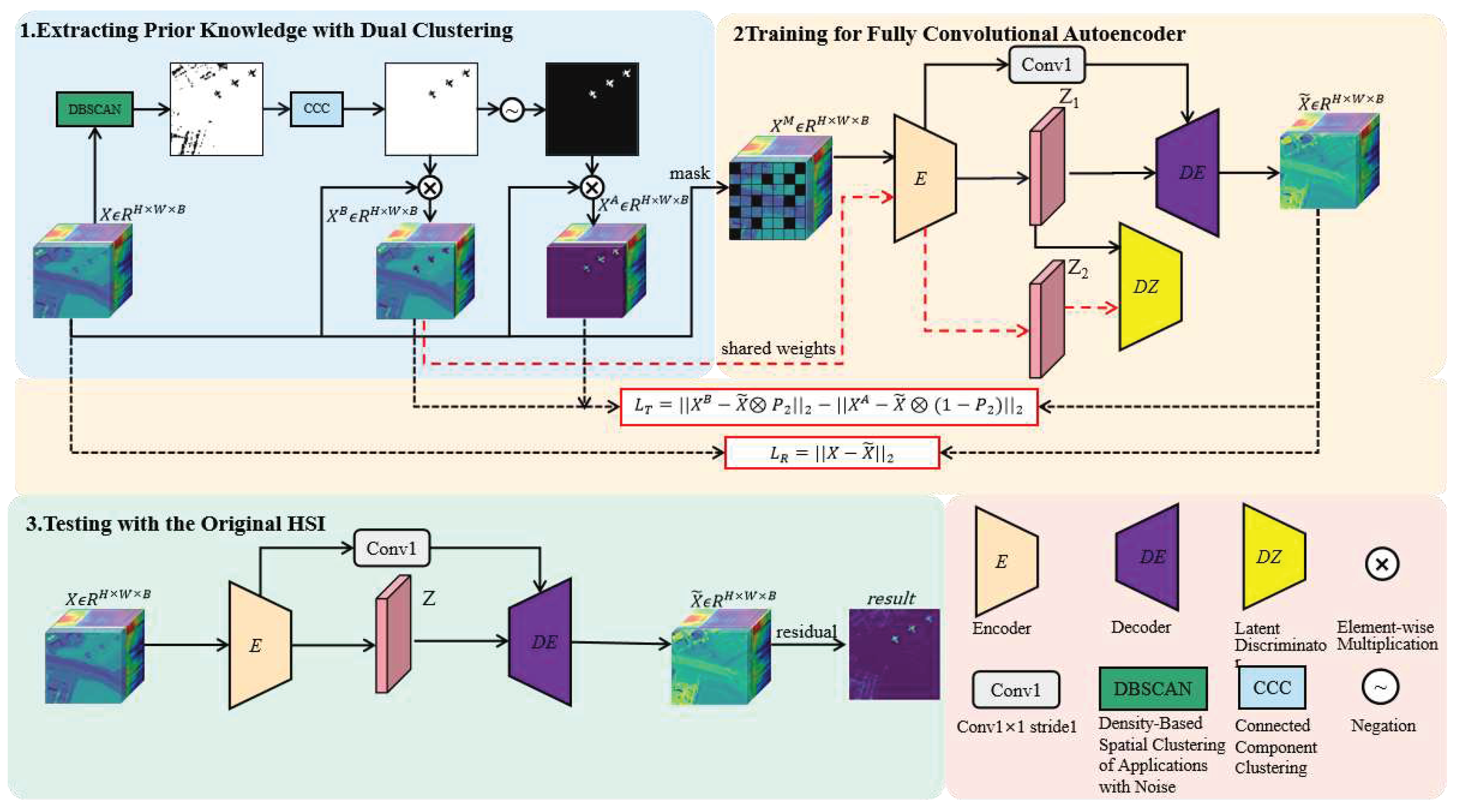
Figure 2.
Flowchart of the dual clustering.
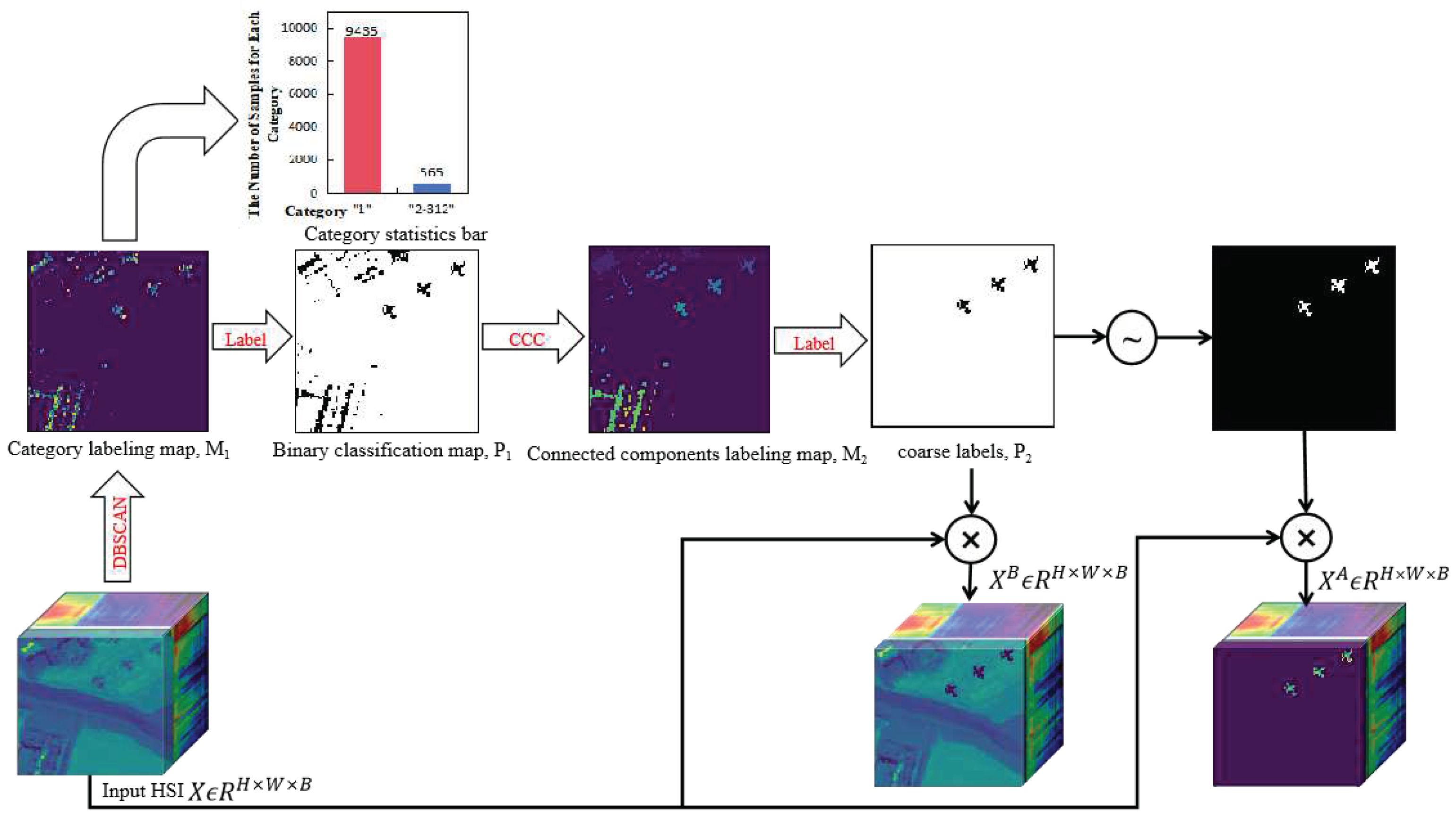
Figure 3.
Detailed deep network architecture of FCAE for hyperspectral anomaly detection: (a) Fully Convolutional Auto-Encoder; (b) EresConvblock; (c) DEresConvblock; (d) Spatial Attention; (e) Spectral Attention.
Figure 3.
Detailed deep network architecture of FCAE for hyperspectral anomaly detection: (a) Fully Convolutional Auto-Encoder; (b) EresConvblock; (c) DEresConvblock; (d) Spatial Attention; (e) Spectral Attention.
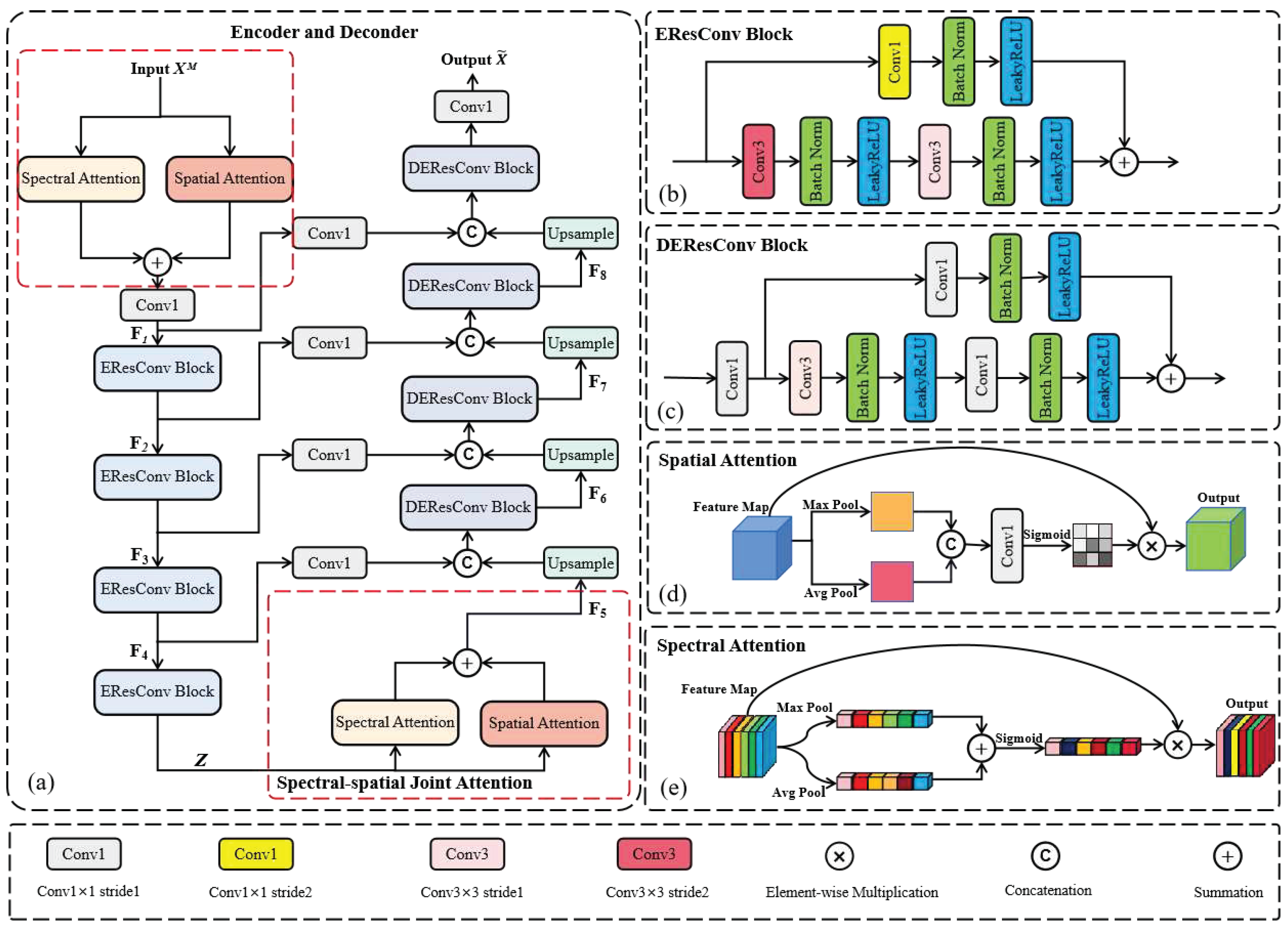
Figure 4.
Detailed deep network architecture of LFACN: (a) Latent Feature Adversarial Consistency Network; (b) Latent Discriminator .
Figure 4.
Detailed deep network architecture of LFACN: (a) Latent Feature Adversarial Consistency Network; (b) Latent Discriminator .
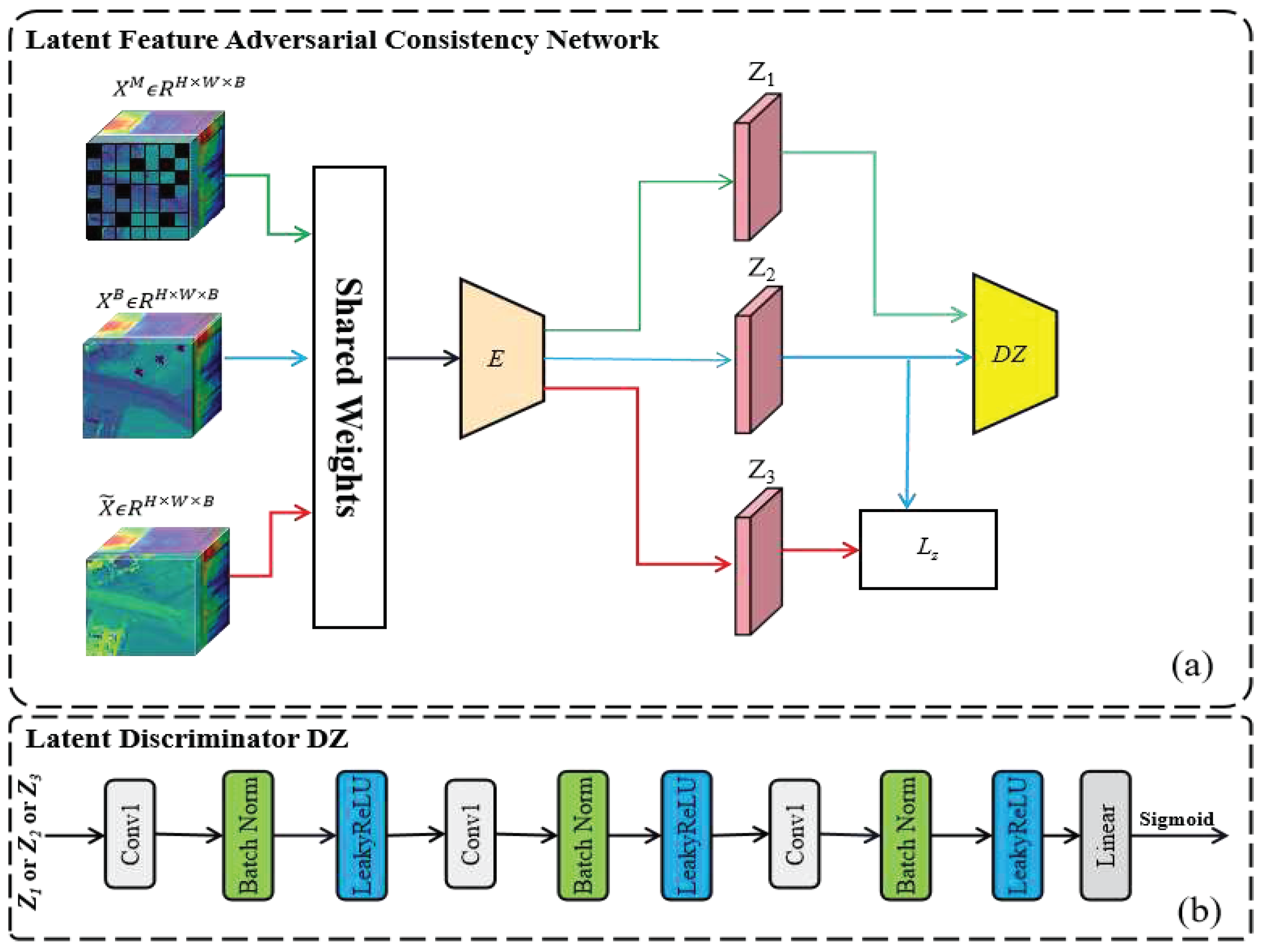
Figure 5.
Pseudocolor images and ground-truth maps of seven experimental hyperspectral datasets: (a) San Diego airport; (b) San Diego-1; (c) San Diego-2; (d) San Diego-3; (e) HYDICE; (f) Pavia; (g) LA-1; (h) Gulfport.
Figure 5.
Pseudocolor images and ground-truth maps of seven experimental hyperspectral datasets: (a) San Diego airport; (b) San Diego-1; (c) San Diego-2; (d) San Diego-3; (e) HYDICE; (f) Pavia; (g) LA-1; (h) Gulfport.
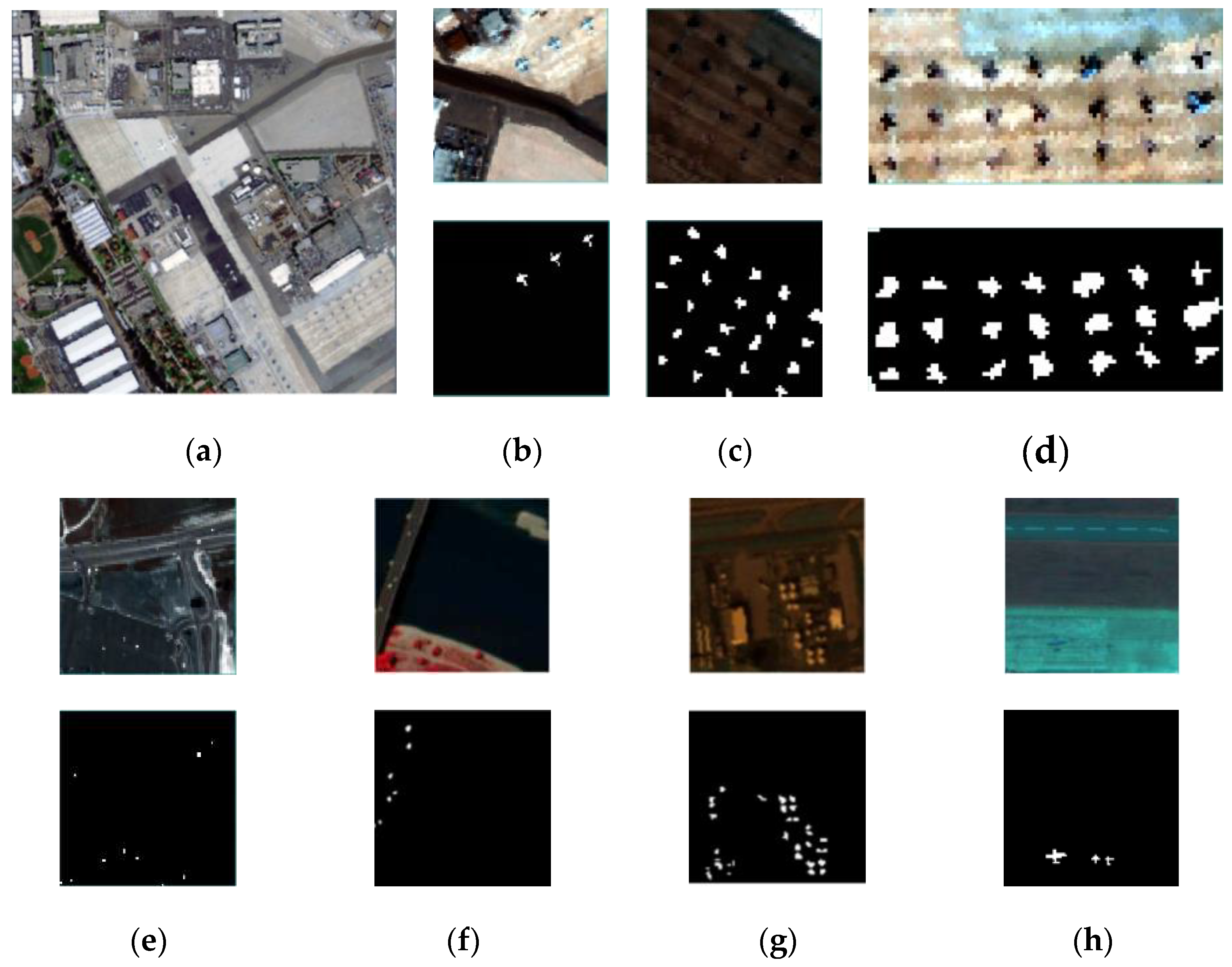
Figure 6.
Heat maps obtained by different algorithms on the San Diego-1: (a) Ground truth; (b) GRX; (c) LRX; (d) FRFE; (e) CRD; (f) AED; (g) LRASR; (h) GAED; (i) RGAE; (j) Auto-AD; (k) Ours.
Figure 6.
Heat maps obtained by different algorithms on the San Diego-1: (a) Ground truth; (b) GRX; (c) LRX; (d) FRFE; (e) CRD; (f) AED; (g) LRASR; (h) GAED; (i) RGAE; (j) Auto-AD; (k) Ours.
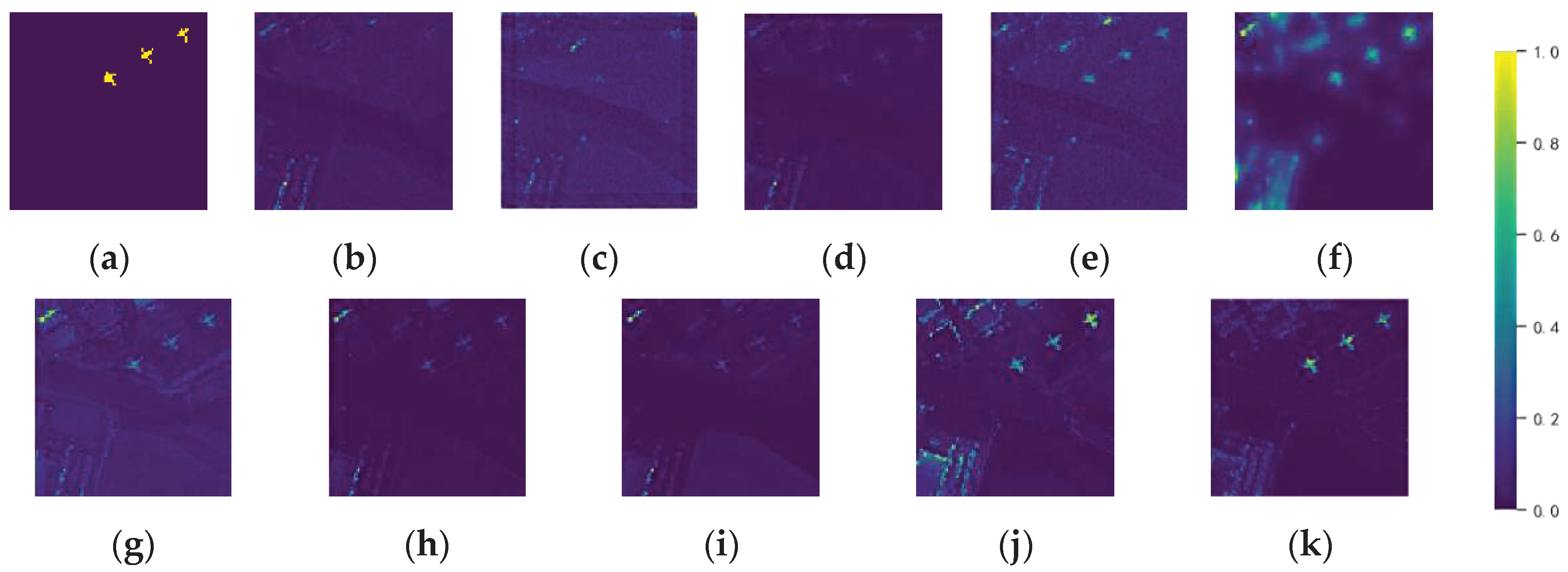
Figure 7.
Heat maps obtained by different algorithms on the San Diego-2: (a) Ground truth; (b) GRX; (c) LRX; (d) FRFE; (e) CRD; (f) AED; (g) LRASR; (h) GAED; (i) RGAE; (j) Auto-AD; (k) Ours.
Figure 7.
Heat maps obtained by different algorithms on the San Diego-2: (a) Ground truth; (b) GRX; (c) LRX; (d) FRFE; (e) CRD; (f) AED; (g) LRASR; (h) GAED; (i) RGAE; (j) Auto-AD; (k) Ours.
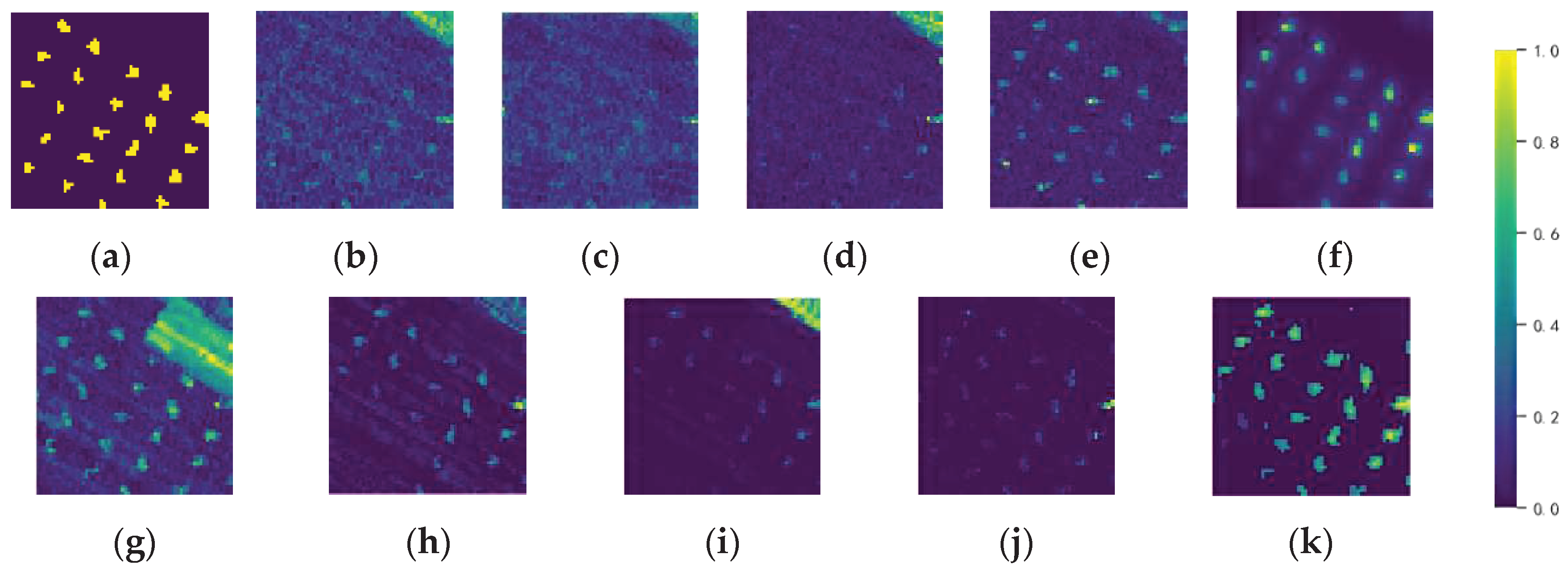
Figure 8.
Heat maps obtained by different algorithms on the San Diego-3: (a) Ground truth; (b) GRX; (c) LRX; (d) FRFE; (e) CRD; (f) AED; (g) LRASR; (h) GAED; (i) RGAE; (j) Auto-AD; (k) Ours.
Figure 8.
Heat maps obtained by different algorithms on the San Diego-3: (a) Ground truth; (b) GRX; (c) LRX; (d) FRFE; (e) CRD; (f) AED; (g) LRASR; (h) GAED; (i) RGAE; (j) Auto-AD; (k) Ours.
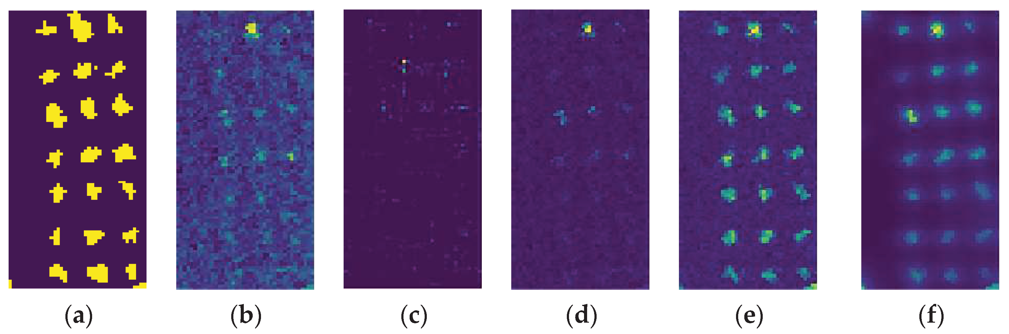
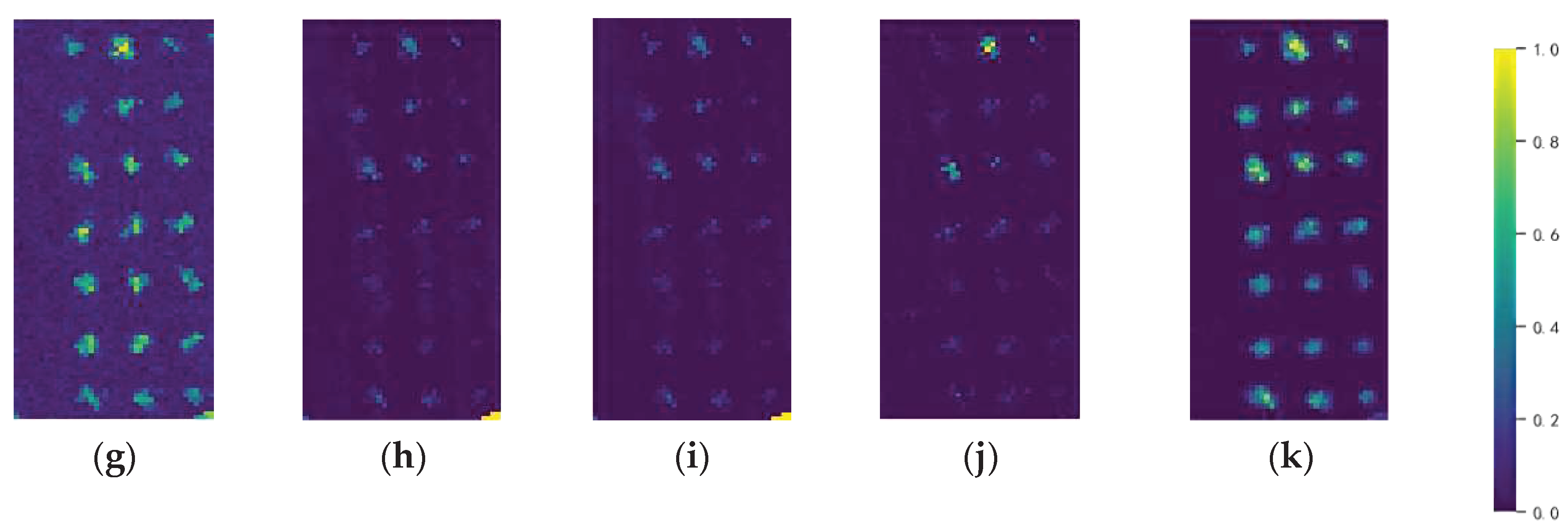
Figure 9.
Heat maps obtained by different algorithms on the HYDICE: (a) Ground truth; (b) GRX; (c) LRX; (d) FRFE; (e) CRD; (f) AED; (g) LRASR; (h) GAED; (i) RGAE; (j) Auto-AD; (k) Ours.
Figure 9.
Heat maps obtained by different algorithms on the HYDICE: (a) Ground truth; (b) GRX; (c) LRX; (d) FRFE; (e) CRD; (f) AED; (g) LRASR; (h) GAED; (i) RGAE; (j) Auto-AD; (k) Ours.
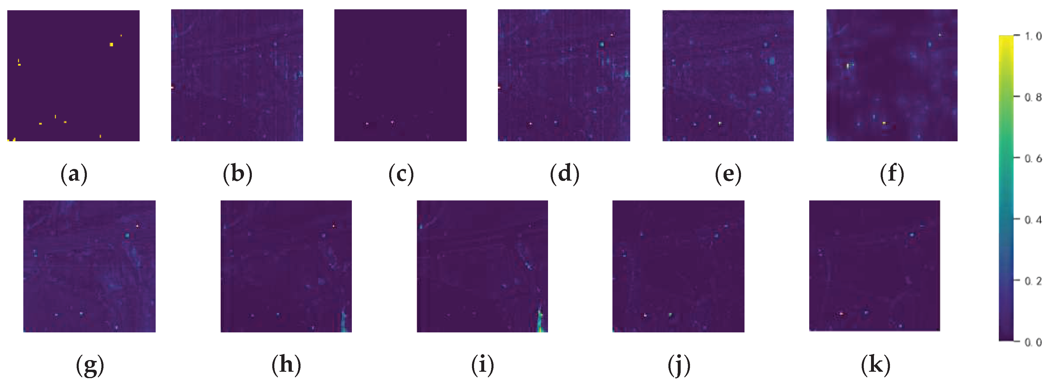
Figure 10.
Heat maps obtained by different algorithms on the Pavia: (a) Ground truth; (b) GRX; (c) LRX; (d) FRFE; (e) CRD; (f) AED; (g) LRASR; (h) GAED; (i) RGAE; (j) Auto-AD; (k) Ours.
Figure 10.
Heat maps obtained by different algorithms on the Pavia: (a) Ground truth; (b) GRX; (c) LRX; (d) FRFE; (e) CRD; (f) AED; (g) LRASR; (h) GAED; (i) RGAE; (j) Auto-AD; (k) Ours.
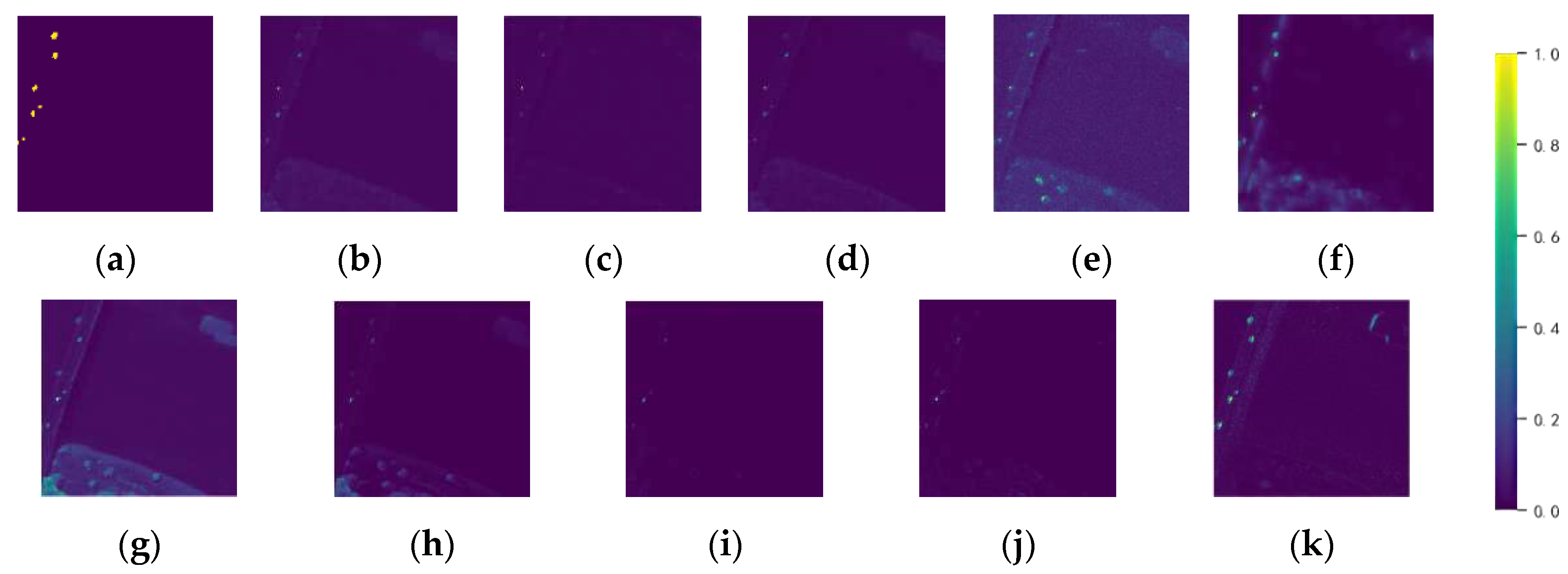
Figure 11.
Heat maps obtained by different algorithms on the LA-1: (a) Ground truth; (b) GRX; (c) LRX; (d) FRFE; (e) CRD; (f) AED; (g) LRASR; (h) GAED; (i) RGAE; (j) Auto-AD; (k) Ours.
Figure 11.
Heat maps obtained by different algorithms on the LA-1: (a) Ground truth; (b) GRX; (c) LRX; (d) FRFE; (e) CRD; (f) AED; (g) LRASR; (h) GAED; (i) RGAE; (j) Auto-AD; (k) Ours.
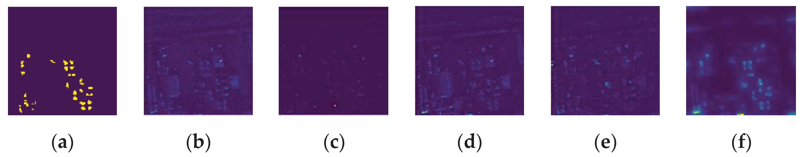
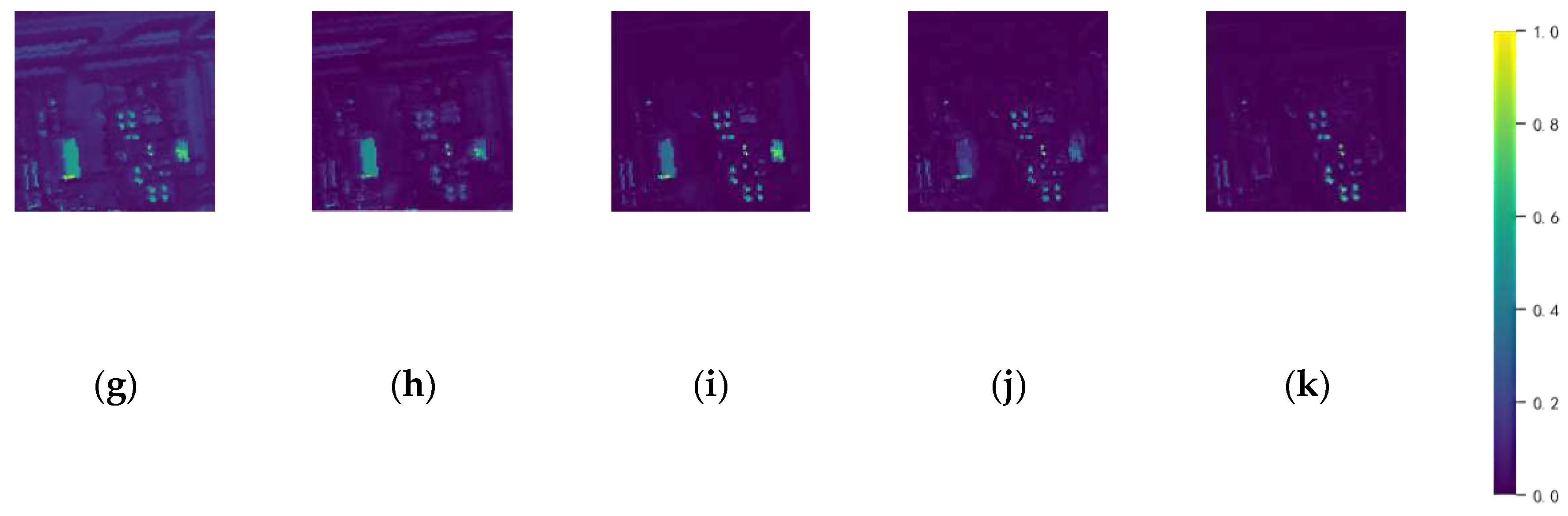
Figure 12.
Heat maps obtained by different algorithms on the Gulfport: (a) Ground truth; (b) GRX; (c) LRX; (d) FRFE; (e) CRD; (f) AED; (g) LRASR; (h) GAED; (i) RGAE; (j) Auto-AD; (k) Ours.
Figure 12.
Heat maps obtained by different algorithms on the Gulfport: (a) Ground truth; (b) GRX; (c) LRX; (d) FRFE; (e) CRD; (f) AED; (g) LRASR; (h) GAED; (i) RGAE; (j) Auto-AD; (k) Ours.
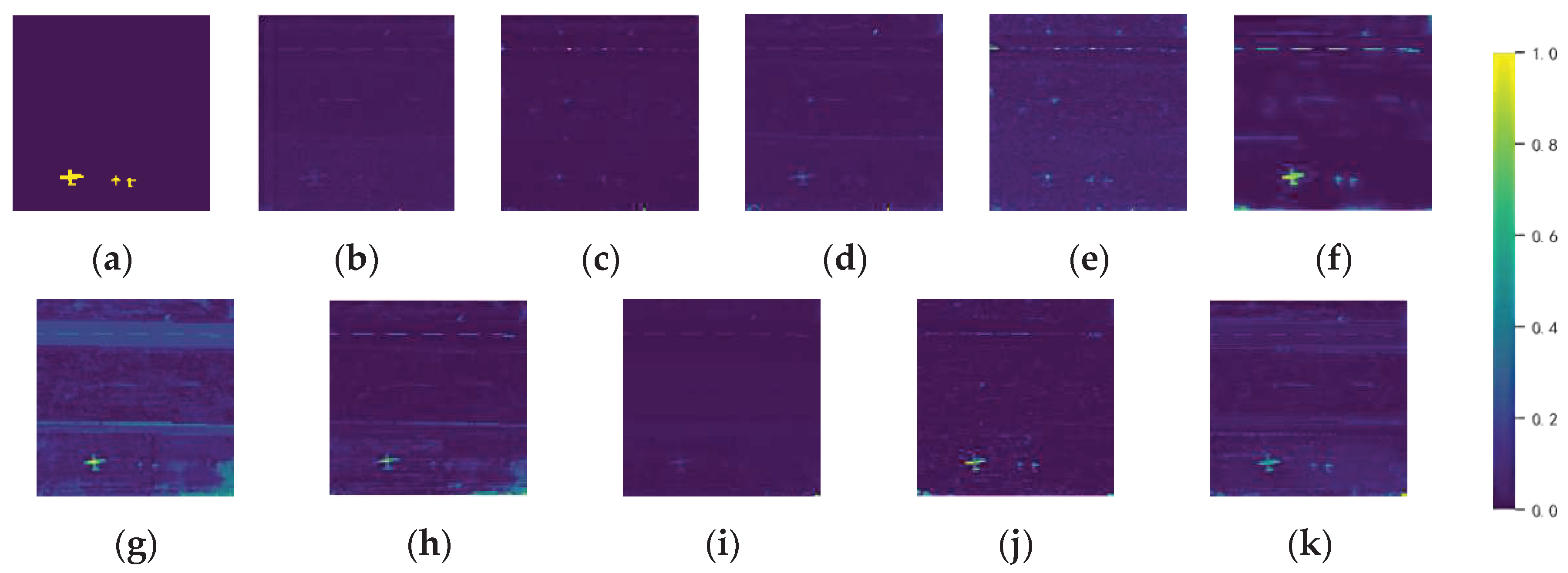
Figure 13.
ROC curves for different detectors on the seven considered datasets: (a) San Diego-1; (b) San Diego-2; (c) San Diego-3; (d) HYDICE; (e) Pavia; (f) LA-1; (g) Gulfport.
Figure 13.
ROC curves for different detectors on the seven considered datasets: (a) San Diego-1; (b) San Diego-2; (c) San Diego-3; (d) HYDICE; (e) Pavia; (f) LA-1; (g) Gulfport.
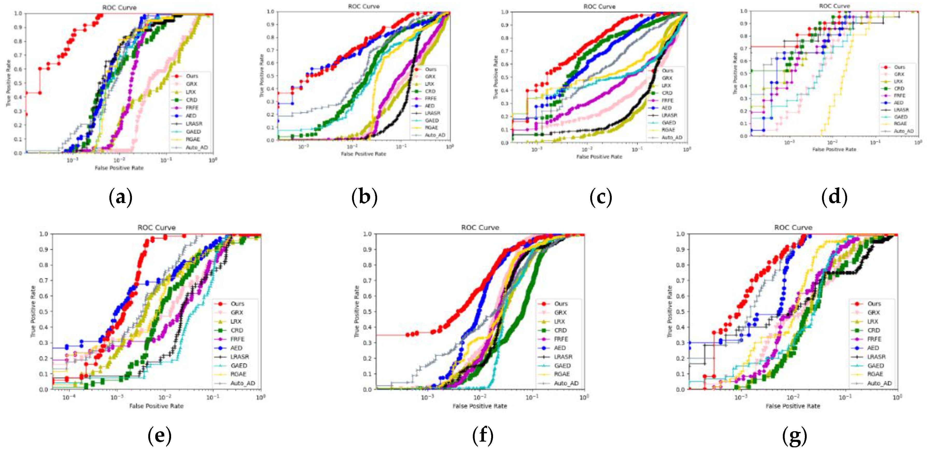
Figure 14.
Separability boxplots for different detectors on the seven considered datasets: (a) San Diego-1; (b) San Diego-2; (c) San Diego-3; (d) HYDICE; (e) Pavia; (f) LA-1; (g) Gulfport.
Figure 14.
Separability boxplots for different detectors on the seven considered datasets: (a) San Diego-1; (b) San Diego-2; (c) San Diego-3; (d) HYDICE; (e) Pavia; (f) LA-1; (g) Gulfport.
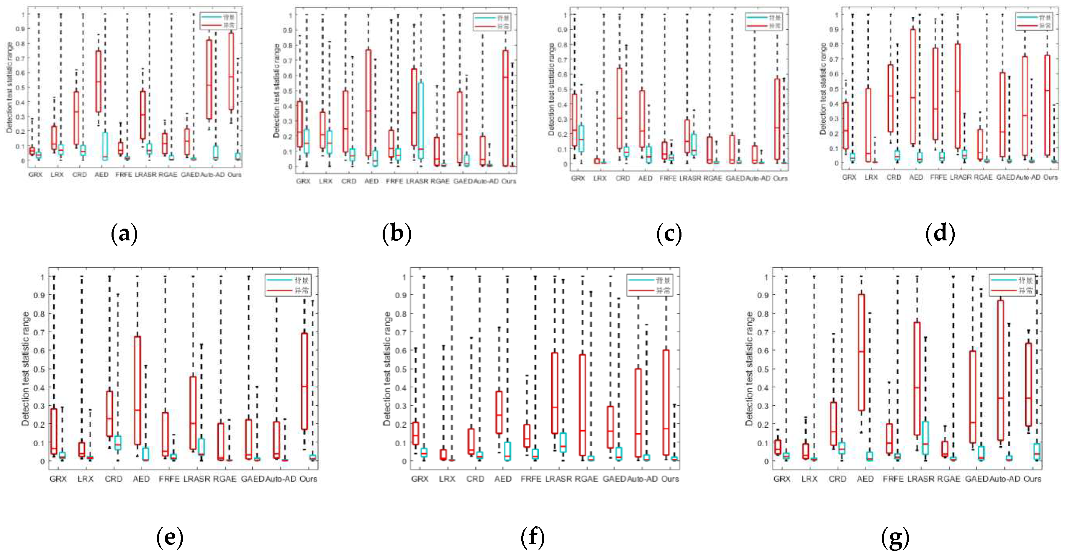
Figure 15.
Analysis of the parameters with all the experimental datasets: (a) clustering radius Eps; (b) MinPts; (c) filtering threshold .
Figure 15.
Analysis of the parameters with all the experimental datasets: (a) clustering radius Eps; (b) MinPts; (c) filtering threshold .
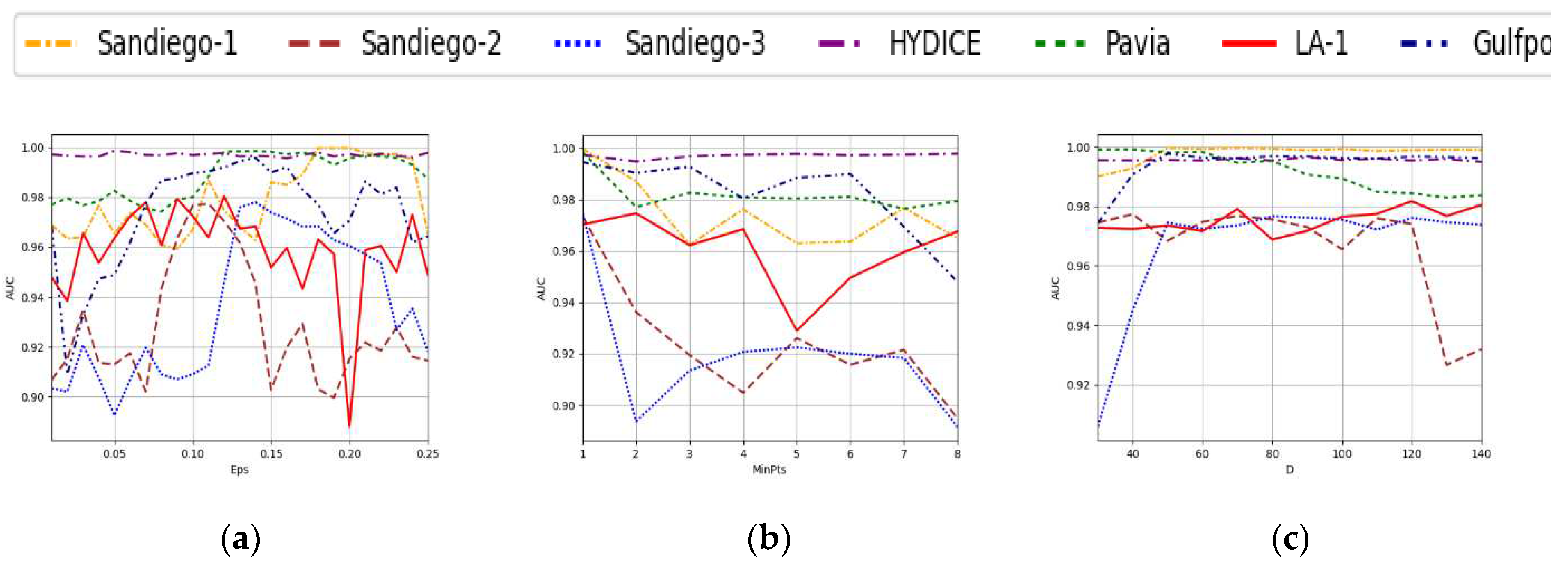
Figure 16.
Effects of the parameters () over the AUC scores of () on each dataset.
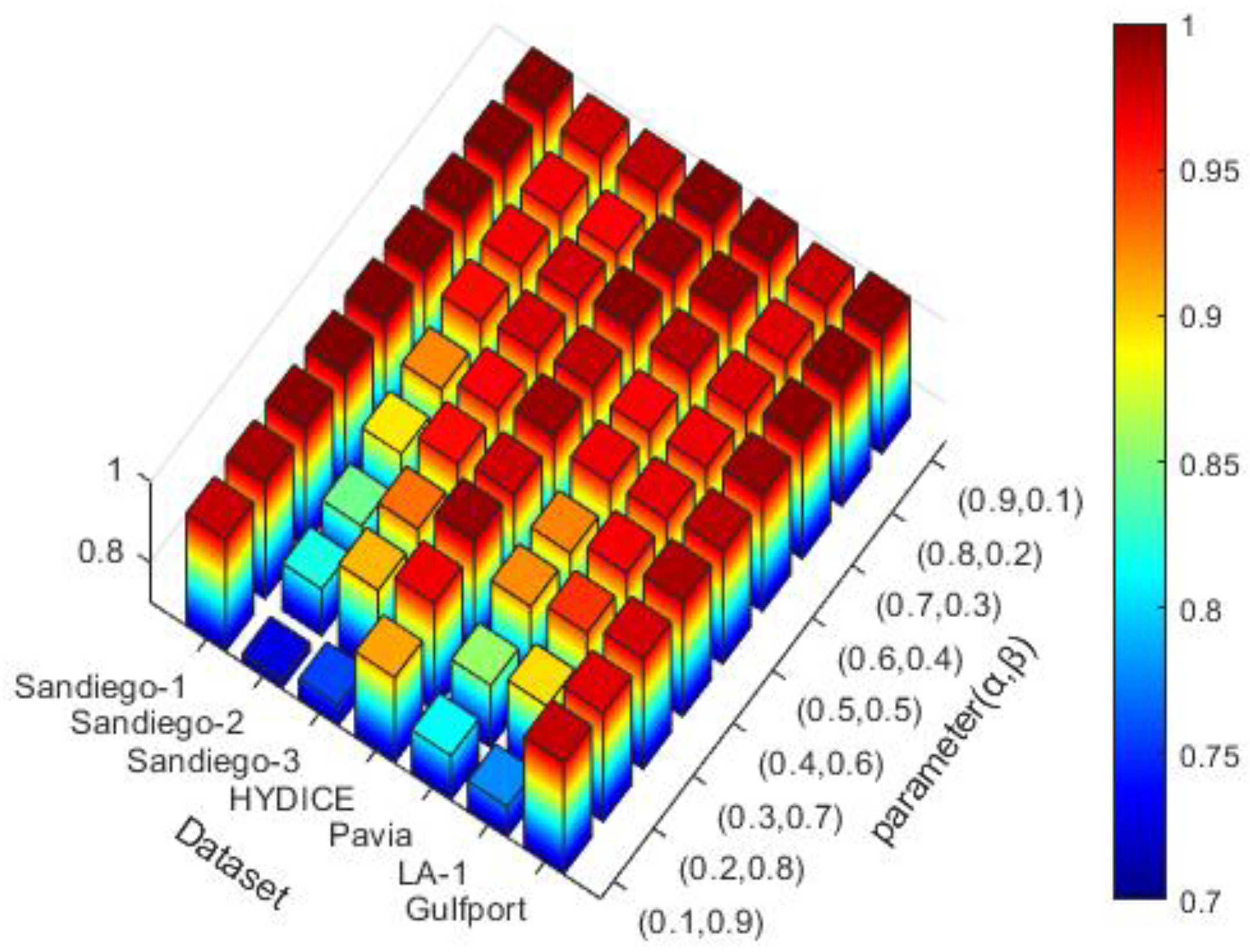

Table 1.
The AUC values of the 10 considered detectors on different datasets.
| Dataset | of Different Methods | |||||||||
|---|---|---|---|---|---|---|---|---|---|---|
| GRX | LRX | FRFE | CRD | AED | LRASR | GAED | RGAE | Auto-AD | Ours | |
| Sandiego-1 | 0.8736 | 0.8570 | 0.9787 | 0.9768 | 0.9900 | 0.9824 | 0.9861 | 0.9854 | 0.9895 | 0.9994 |
| Sandiego-2 | 0.7499 | 0.7211 | 0.7821 | 0.9290 | 0.9399 | 0.8065 | 0.8905 | 0.8819 | 0.9466 | 0.9773 |
| Sandiego-3 | 0.7125 | 0.7540 | 0.7694 | 0.9485 | 0.9659 | 0.7214 | 0.7811 | 0.8341 | 0.9163 | 0.9815 |
| HYDICE | 0.9857 | 0.9911 | 0.9933 | 0.9976 | 0.9951 | 0.9744 | 0.9843 | 0.9646 | 0.9951 | 0.9980 |
| Pavia | 0.9538 | 0.9525 | 0.9457 | 0.9510 | 0.9793 | 0.9380 | 0.9398 | 0.9688 | 0.9914 | 0.9979 |
| LA-1 | 0.9692 | 0.9492 | 0.9655 | 0.9229 | 0.9780 | 0.9440 | 0.9424 | 0.9569 | 0.9406 | 0.9808 |
| Gulfport | 0.9526 | 0.9532 | 0.9722 | 0.9342 | 0.9953 | 0.9120 | 0.9705 | 0.9842 | 0.9968 | 0.9975 |
| Average | 0.8853 | 0.8826 | 0.9153 | 0.9514 | 0.9777 | 0.8970 | 0.9278 | 0.9394 | 0.9680 | 0.9903 |
Table 2.
The AUC values of ablation Study on different datasets.
| Component | of different cases | ||||||
|---|---|---|---|---|---|---|---|
| Sandiego-1 | Sandiego-2 | Sandiego-3 | HYDICE | Pavia | LA-1 | Gulfport | |
| FCAE without SSJA | 0.9732 | 0.8785 | 0.8567 | 0.9887 | 0.9600 | 0.9168 | 0.9679 |
| FCAE | 0.9786 | 0.8864 | 0.8630 | 0.9920 | 0.9686 | 0.9229 | 0.9763 |
| FCAE+ | 0.9975 | 0.9221 | 0.9336 | 0.9961 | 0.9881 | 0.9669 | 0.9822 |
| FCAE++ LFACN | 0.9996 | 0.9763 | 0.9722 | 0.9979 | 0.9932 | 0.9791 | 0.9957 |
Table 3.
The Inference Time of different detectors.
| Dataset | Inference Time of different detectors | |||||||||
|---|---|---|---|---|---|---|---|---|---|---|
| GRX | LRX | FRFE | CRD | AED | LRASR | GAED | RGAE | Auto-AD | Ours | |
| Sandiego-1 | 0.2146 | 9.1735 | 9.8865 | 3.9145 | 0.2107 | 46.3339 | 0.0305 | 0.0335 | 0.0210 | 0.0390 |
| Sandiego-2 | 0.3168 | 25.6535 | 14.9289 | 5.0192 | 0.2456 | 57.3001 | 0.0394 | 0.0570 | 0.0275 | 0.0185 |
| Sandiego-3 | 0.0998 | 18.2074 | 5.4494 | 2.1902 | 0.1884 | 19.2353 | 0.0150 | 0.0157 | 0.0160 | 0.0210 |
| HYDICE | 0.2146 | 9.1735 | 9.8865 | 3.9145 | 0.2107 | 46.3339 | 0.0305 | 0.0335 | 0.0210 | 0.0235 |
| Pavia | 0.9823 | 16.8106 | 33.5833 | 5.3146 | 0.3625 | 61.1938 | 0.1072 | 0.0476 | 0.0305 | 0.0355 |
| LA-1 | 0.3173 | 14.2751 | 21.3859 | 5.3762 | 0.2242 | 72.0277 | 0.0345 | 0.0459 | 0.0240 | 0.0330 |
| Gulfport | 0.5988 | 13.7447 | 13.6096 | 5.0287 | 0.2652 | 63.4349 | 0.0620 | 0.0373 | 0.0220 | 0.0275 |
| Average | 0.3771 | 14.6755 | 14.9511 | 4.1165 | 0.2563 | 48.4835 | 0.0436 | 0.0366 | 0.0229 | 0.0283 |
Disclaimer/Publisher’s Note: The statements, opinions and data contained in all publications are solely those of the individual author(s) and contributor(s) and not of MDPI and/or the editor(s). MDPI and/or the editor(s) disclaim responsibility for any injury to people or property resulting from any ideas, methods, instructions or products referred to in the content. |
© 2024 by the authors. Licensee MDPI, Basel, Switzerland. This article is an open access article distributed under the terms and conditions of the Creative Commons Attribution (CC BY) license (http://creativecommons.org/licenses/by/4.0/).
Copyright: This open access article is published under a Creative Commons CC BY 4.0 license, which permit the free download, distribution, and reuse, provided that the author and preprint are cited in any reuse.


