Submitted:
20 October 2025
Posted:
20 October 2025
You are already at the latest version
Abstract
Accurate prediction of train acceleration is an essential requirement for Automatic Train Operation (ATO) in urban railways. While traditional single-point mass models fail to capture the distributed dynamics of coupled vehicles, multi-point models are rarely practical due to their computational cost. In this paper, we propose an enhanced single-point mass model based on Long Short-Term Memory (LSTM) networks. The model is trained on Train Control and Monitoring System (TCMS) data from Busan Metro Line 3. By averaging the coupled dynamics of sequence-cars, we obtain a realistic single-point representation. The input data undergoes kinematic preprocessing and feature engineering, including lagging, cross, and statistical measurements. The key innovation of this paper is the physics-based feedback loop mechanism, which is built into the LSTM. This mechanism uses the predicted train acceleration at each time step to update systematically the acceleration-dependent features and make new predictions. This maintains physical consistency and causal relationships without requiring future measurements, reflecting the real-world ATO operational limits. Results demonstrate very high accuracy (R² = 0.9993, MAE = 0.0083 km/h²) without error accumulation, suggesting benefits for both ATO control accuracy and energy efficiency.
Keywords:
long short-term memory (LSTM)
; train dynamic model
; single-point mass model
; train control and monitoring system (TCMS)
; automatic train operation (ATO)
1. Introduction
Automatic Train Operation (ATO) systems play an important role for the modern urban trains as it can automatically execute the driving sequences, such as acceleration and deceleration, from station departure to precise stopping at the next station [1]. The ATO system continuously analyzes the current power status and determines the required compensatory power commands, which are executed through the Train Control and Monitoring System (TCMS). The TCMS generates the corresponding traction and braking forces through the coordinated operation of the traction motors, the regenerative braking systems, and the friction braking systems, directly influencing the final acceleration and speed profiles of the urban trains [2]. Therefore, precise control of the motion of the urban trains fundamentally requires the accurate dynamic models capable of the predicting train acceleration response under diverse operational conditions [3,4].
However, the forces acting on the urban trains exhibit extreme complexity, arising from the multiple interacting factors, including the air resistance, the rolling resistance, the gradient resistance, and the curve resistance [5]. Even with the theoretically complete dynamic models, the characteristics and the responses of the system can inevitably vary with the vehicle aging, the mechanical wear, and the environmental conditions [6]. The actual train resistance can diverge significantly from the generalized train resistance due to the various factors, such as the operational disturbances [7], the mechanical tolerances, and seasonal variations in temperature and humidity [8]. These discrepancies between the theoretical predictions and the actual operational behavior reveal the fundamental limitations of the conventional dynamic models applied to the design of the ATO system.
Traditional methods use either single-point or multi-point mass models to predict the dynamics of the train systems. The single-point mass models simplify the dynamics by considering the entire train system as a concentrated mass and combining the force balance equations. However, this approach leaves out the important distributed effects that occur along the train, such as the forces between connected vehicles, differences in braking behavior, and the resulting longitudinal vibrations [9]. Therefore, this simplified approach fails to capture the complex dynamic interactions that occur among the sequence-cars. This limitation can be addressed by using the multi-point mass models, which represent the individual cars with coupling dynamics and achieve a higher prediction fidelity [10,11,12]. However, the computation cost still limits these models in real-time ATO systems. To address these limitations, recent research has increasingly adopted deep learning and AI approaches to capture and model the complex train dynamics, while preserving computational efficiency [13,14,15,16].
Deep learning and artificial intelligence (AI) influences as the main topics of recent research in the field of urban trains. Short-Term Memory (LSTM) networks have demonstrated particular effectiveness for time series prediction tasks involving temporal dependencies [17,18]. Several studies have investigated the data-driven approaches for the applications of the urban trains, including trajectory prediction [19,20], fault detection applications [21], virtual coupling [22], and comfort prediction [23]. However, existing approaches either lack the physical rules [24] or require the explicit dynamic model formulations, which limit their ability to capture the unmodeled disturbances across different operational scenarios and track characteristics [25,26]. Moreover, they needed to achieve the prediction fidelity while maintaining computational efficiency, which is suitable for real-time ATO applications [27].
This paper presents an enhanced single-point mass dynamic model for the prediction of the train acceleration, based on Long Short-Term Memory (LSTM) that incorporates the physics-based feedback mechanisms. The model is trained using the operational data from 16 track sections covering 17 stations on Busan Metro Line No.3. This data represents a realistic single-point by averaging the coupled dynamics of sequence-cars and also includes a variety of operational scenarios under real-world ATO conditions, such as varying track geometries, environmental factors, and disturbances. Firstly, the input data are prepared using a kinematic-based preprocessing methodology that ensures physical consistency through acceleration derivation, followed by a moving average filter. Then, the comprehensive feature engineering framework is implemented to create the temporal representations through lagging, cross, and statistical features to provide the accuracy of the prediction of the proposed model. The LSTM-based train dynamic model is strategically built in two phases: the training phase and the evaluation phase. The novel physics-based feedback mechanism is implemented into the LSTM to inform the predicted acceleration value for the subsequent predictions, reflecting real-world operational constraints. The comprehensive validation across 16 diverse track sections demonstrates the robust generalization and exceptional accuracy (R² = 0.9993, MAE = 0.0083 km/h²). Therefore, the proposed model can address the practical requirements of ATO systems, such as disturbance mitigation and precise automatic driving control in urban rail system automation.
This paper is organized into five sections. The next section briefly reviews the theoretical background of parametric dynamic models and introduces the definition of a dynamic model based on artificial intelligence (AI). Chapter 3 describes the implementation of the proposed enhanced single-point mass model based on LSTM and explains the design of the underlying train dynamics model. Chapter 4 presents the evaluation results of the proposed model. Finally, Chapter 5 concludes this paper.
2. Methodology
2.1. Problem Statement
The design of the ATO algorithm requires not only various characteristics affecting the movement of the train, but also a very high-precision dynamic modeling that reflects the unique characteristics of the braking system, considering the stopping function at the designated location on the platform [28].
A second problem is that even when modeling incorporates external disturbances to the greatest extent possible, errors in the electrical and mechanical characteristics of components from the same manufacturer can still occur, requiring operators to individually tune each train to match the original standard design values. This increases management costs. To address this issue, urban rail operators are demanding a system that enables automatic operation (ATO) for all trains based on their own dynamic modeling.
Railway vehicle dynamics is the analysis of various dynamic characteristics that appear due to friction adhesion between wheels and rails, various mechanical friction, traction characteristics, braking characteristics, the weight of each vehicle, various vibrations that occur during operation, and the gradient and curve of the track. The dynamic characteristics of a train can be divided into lateral dynamics in the left-right direction, longitudinal dynamics in the track direction, and vertical models for up-and-down movement, depending on the phenomenon.[29]. In addition, in terms of the parametric approach, it is divided into a single-mass model and a multi-mass model that separately consider each parameter of a connected vehicle.
The single-mass model assumes that the mass distribution of multiple connected urban trains is constant, and the focus of the mass is considered to be in the middle of the vehicle. Although this model cannot accurately represent the internal characteristics generated by the coupled system, it can easily understand the acceleration/deceleration motion along the longitudinal track, so it is easy to mathematically express the force acting on the train along the direction of motion to capture the transient motion [30]. Therefore, it has the advantage of simplifying calculations and increasing the possibility of system implementation, and is widely used in urban railway automatic train operation (ATO) research [31].
The multi-mass model takes into account all the characteristics of the parameters between multiple connected sequence-cars. This method analyzes the direction and influence of various forces acting on each vehicle during the operation of multiple connected sequence-cars, such as when starting, stopping, going through a gradient, or passing a curve, by element, or interprets the force acting on the train coupling device from the perspective of compression and tension. It is used for research on improving ride comfort by sequentially alleviating shocks during towing or braking, and preventing vehicle separation or derailment due to damage to the coupler. However, it has the disadvantage of being very computationally complex.
Recent research on automatic train operation (ATO) for urban railways heavily relies on single-point mass models, and the multi-point models can be viewed as an optimized or extended version of this model. This model is expressed as follows:[26]
where, represents the total mass of the train, and denote the train traction force, and the train braking force, and refer to the relative acceleration and braking coefficients, respectively. is the Davis formula, which represents the relationship between train speed and air resistance, and , , and represent resistance parameters. and represent the gradient resistance, and the curve resistance, respectively.
2.2. Train Dynamics Model Based on LSTM
This study aims to develop a dynamic model using actual data from the automated operation (ATO) of Busan Metro Line No.3. This ATO data contains a variety of resistance values (disturbances) that cannot be captured by parametric train dynamic models, allowing for transformation into the most complete dynamic model. Artificial Intelligence (AI) is a field of technology that enables computer systems to perform various advanced functions by mimicking human learning, reasoning, and perception. Rapid computer advancements are shaping AI technology as a core technology driving a new industrial era, and it is being widely utilized in areas such as autonomous driving, medical diagnosis, object recognition and classification, and finance [32,33]. In the railway industry, AI is emerging in the form of reinforcement learning-based automatic operation (ATO) control [34] and deep learning-based driving pattern learning model development [35], and is expected to become a new driving force for future railway development.
The data provided in this study are operational records related to autonomous train operation, containing a wide range of information. However, structuring the data is challenging. Therefore, applying machine learning models is challenging, requiring consideration of the field of deep learning. Machine learning models are designed to learn from structured data to make accurate predictions and decisions. However, if the data is not accurately labeled, the model cannot accurately understand the data. This problem can be solved by deep learning [36]. Deep learning models utilize multilayer artificial neural networks that mimic the neural network structure of the human brain to process data, automatically extract features, and enable learning and prediction [19]. Therefore, they are considered highly useful for building dynamic models.
The next consideration is the characteristics of the data. The characteristic of driving data is that it is entered in chronological order, from start to stop. The goal of this data is to nonparametrically explore, learn, and predict dynamic changes occurring during driving, thereby extracting a dynamic model. Therefore, we utilized a long-short-term memory (LSTM) neural network, which has shown excellent performance in solving time-series problems. The LSTM network is an advanced recurrent neural network with the additional ability to maintain memory of previous inputs, and has shown good performance in handling time-series problems such as train dynamic models and speed prediction. The LSTM neural network model that interprets railway operation data will be a useful tool for studying dynamic models that do not require various parameters and mechanical numerical inputs. In this paper, statics elements were excluded from the train data provided for dynamic model extraction, and dynamic elements defined in the parametric model were selected and input.
3. Implementation of the Proposed Train Dynamic Model
3.1. Architecture of LSTM Network
In 1997, Hochreiter and Schmidhuber first introduced the Long Short-Term Memory (LSTM) [37], which is an improved version of the recurrent neural network (RNN). A single hidden state in the traditional RNNs can vanish the information for the long term. LSTM can address this problem by introducing a memory cell to hold information for an extended period. Therefore, LSTM architectures are capable of learning long-term dependencies in sequential data, which is valuable for applications of time series analysis and other temporal pattern recognition tasks.
For train acceleration prediction, LSTM demonstrates particular effectiveness due to its ability to capture long-term temporal dependencies inherent in railway operational dynamics, where current acceleration states depend on historical speed profiles, track conditions, and control inputs. The LSTM architecture is shown in Figure 1 as follows:
The forget gate calculates values between 0 and 1 to decide what information should be erased or kept for future use from the previous cell state:
Using a sigmoid activation function, the input gate decides what new information should be saved in the cell state:
where the sigmoid activation function is:
The candidate memory cell creates a vector of new candidate values using a hyperbolic tangent activation function, which is as follows:
where the tanh activation function is:
The new cell state is the combination of the information from the forget gate and the new candidate memory cell:
The output gate determines which parts of the cell state should result as the hidden state:
Finally, the hidden state is the cell state to serve as both the current output and input for the next time step:
3.2. Preparation of Data
3.2.1. Data Collection
In this study, we collected the comprehensive datasets of the actual in-field data, which were gathered through the “Train Control and Monitoring System (TCMS)” from Busan Metro Line No.3 with a total of 16 track sections of all 17 stations from April 2020 and December 2022. Each track section has 21 datasets, which are collected randomly at different times, weather conditions, and external disturbances to provide high-resolution operational insights and reflect real-world operational diversity. The ATO operation data from the Train Control & Monitoring System (TCMS) provides aggregated traction and braking forces across four sequence cars, although each operates independently [38,39]. The resulting acceleration data averages across four sequence cars, which reflects multi-point mass dynamics, offering greater accuracy than a single-point mass model. By incorporating real running disturbances, the proposed dynamic model reduces external influences, improves automatic driving precision, and supports more efficient ATO equipment management, thereby advancing future functionality in urban railways. The dataset architecture divides the data into the training and testing datasets.
3.2.2. Data Preprocessing
In the real-world workspace, failures, faults, and noise in sensors or actuators can lead to missing data. The LSTM-based algorithms may result in poor performance of regression and prediction due to the model bias and fitting effect. Therefore, the missing value in deep learning neural networks is still a challenging problem to obtain a more robust, optimized predictive dynamic train model. In this paper, the missing value treatment follows a sequential strategy, which begins with the forward fill to maintain temporal continuity and is followed by the backward fill to address remaining gaps. For the completely missing information, we drop the rows.
The next phase of data preprocessing entails the computation of the acceleration, followed by the moving average filter, relating velocity change to displacement:
where and are consecutive velocity measurements and is the displacement. This physics-based approach ensures that the derived acceleration values accurately reflect the underlying train dynamics while maintaining consistency across different operational scenarios.
3.2.3. Feature Engineering
In this paper, a robust characterization of temporal dynamics and complex nonlinear relationships based on the input data features is constructed through feature engineering. It can help improve the quality of the results of regression and prediction of the LSTM neural network through short-term dynamics and long-term patterns [40]. Lagging features are provided to capture historical context or patterns by incorporating previous time steps:
where represents the lag step, ranging from 1 to 5. Then, the cross features capture the complex relationships and dependencies between consecutive time steps:
Statistical features provide the temporal information about the characteristics of the data through rolling window calculations:
where represents the window size (5, 10, or 20 time steps). First-last difference features capture trend information:
3.2.4. Data Normalization
After finishing the feature engineering procedure and before training the LSTM train dynamic model, data normalization is also a critical step in a data-driven model in order to prevent unbalanced input features, which can lead to uneven weight distribution and affect training performance. In this paper, the “MinMaxScaler” function is used to transform all input features to the range [0, 1], ensuring an equal contribution during model training:
3.2.5. Loss Function and Evaluation Metrics
The model optimization employs “Mean Absolute Error” (MAE) as the primary loss function in this paper:
where represents actual acceleration values and denotes predicted acceleration values. Model performance is evaluated by using Root Mean Squared Error (RMSE) and R-squared (R²) as key metrics. Root Mean Square Error (RMSE) emphasizes larger prediction errors:
The coefficient of determination (R²) quantifies the proportion of variance explained by the model:
where is the mean of actual values.
3.2.6. Hyperparameters
The hyperparameters impact the quality and accuracy of the predicted results. Therefore, the tuning of the hyperparameters is also important [41]. In this paper, we used 64 hidden units per layer to ensure sufficient capacity, which can capture the temporal patterns. Then, the two-LSTM layer structure is set up. The first layer captures the temporal dependencies, while the subsequent layer models the higher-order interaction patterns. Dropout regularization at a rate of 0.3 was implemented to prevent overfitting by random neuron suppression. The “Adaptive Moment Estimation” (Adam) optimizer with a learning rate of 0.001 facilitates adaptive gradient-based optimization incorporating a momentum mechanism. A batch size of 128 samples can provide better gradient estimates while maintaining computational feasibility. The training process spans up to 500 epochs with an early stopping mechanism monitoring validation loss with a patience of 30 epochs to prevent the local minima and overfitting.

Table 1.
Tuning of hyperparameters.
| Name of Types | Quantity |
| Hidden size | 64 |
| Number of LSTM layers | 2 |
| Dropout rate | 0.3 |
| Learning rate | 0.001 |
| Batch size | 128 |
| Number of epochs | 500 |
| Number of patience epochs | 30 |
3.3. Design Architecture of the LSTM-Based Train Dynamic Model
The architecture of the proposed model, based on LSTM, is specifically engineered to capture the complex time series-based relationships in the Busan Metro Line No.3’s operational data. It focuses on the physics-based constraints to make the prediction of the train acceleration more accurate. The core of the proposed model is composed of the hierarchical structure of dual-LSTM layers. The first LSTM layer is configured to pass through to the next layers with the full sequence of the hidden states for temporal feature extraction. The mathematical operation of each LSTM layer processes the input sequence , which passes through the gate mechanisms to create the hidden state sequences . Then the final LSTM layer gives only the final hidden state h_n as the output, containing higher-order temporal interactions and long-term dependencies, which can help for accurate acceleration prediction.
Dropout regularization layers are placed after the LSTM layers to specifically address the overfitting problem. This regularization method is critical for time-series applications where the model must generalize across diverse temporal patterns while avoiding memorization of specific sequences. During training, the dropout layer randomly deactivates a fraction of the input neurons to zero. The mathematical expression of the dropout layer is as follows:
where is the input hidden state, is a binary mask, which is sampled from a Bernoulli distribution with a probability where is the dropout rate of 0.3, and denotes element-wise multiplication. The dropout is not used during inference, such as testing or evaluation, and the outputs are scaled by to keep the activation values without dropout.
The Rectified Linear Unit (ReLU) activation layer introduces the non-linearity after the final LSTM layer. The ReLU activation function is defined as:
The activation functions, such as sigmoid and tanh, before ReLU, were saturated. High values are given to 1.0, and small values snap to 0 or -1. This resulted in the vanishing gradient problem. The ReLU activation can address this problem by maintaining gradient flow for positive activations, introducing sparsity in the network representation.
Finally, we add a dense output layer to wrap up the model. This single dense layer takes all the temporal features and then converts them into a prediction of the train acceleration at time step. For model compilation, Mean Absolute Error (MAE) is used as a loss function along with the Adam optimizer with the tuned learning rate.
Cross-validation is critical for verifying the model accuracy in data-driven models. We used “Time Series Split” function that keeps the data in chronological order. This function is used only in training datasets (which is explained in 4.2.1), not in testing datasets, as the training datasets should be split into the training datasets and the validation datasets in order to build a robust trained model. The working principle of “Time Series Split” function is for each fold, we train on all data up to a certain point, then validate on the next chunk of data:
Each fold gets more training data than the previous one, but we always check the performance of the model through validation datasets. In this paper, we used 30 folds to maintain sufficient training datasets in each fold and get a robust performance of cross-validation. After this process, the testing procedure is performed on the testing dataset.
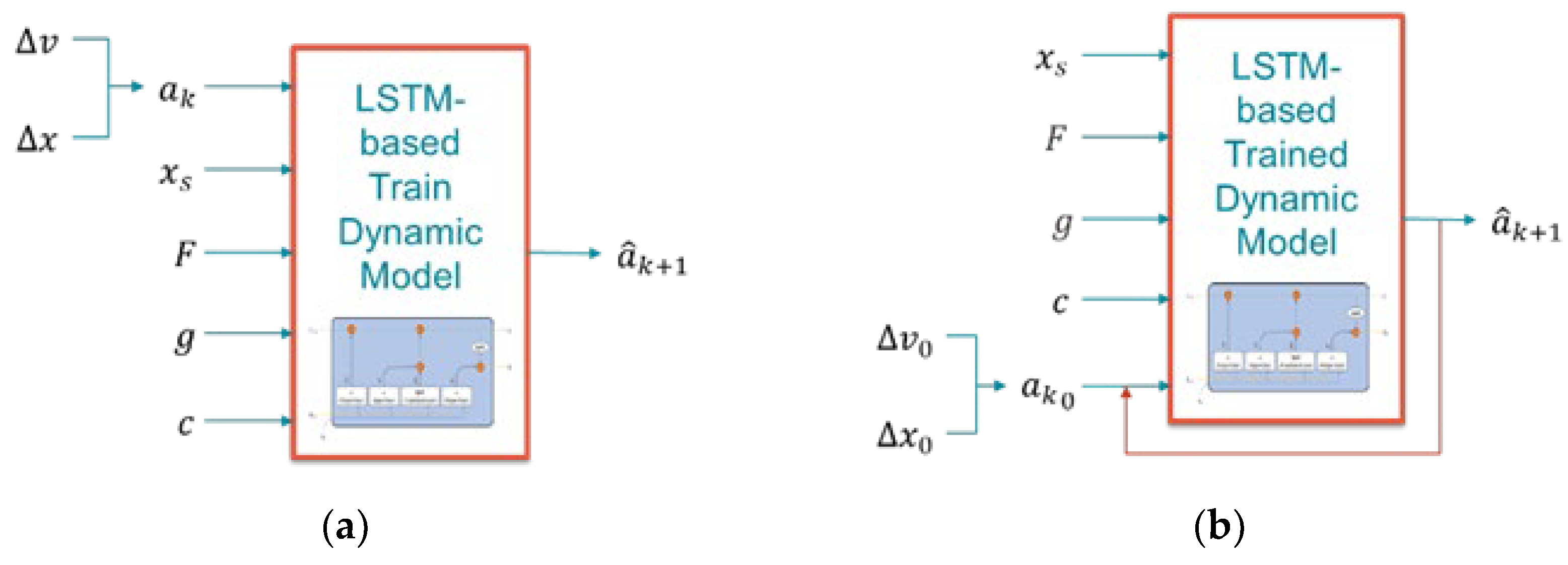
The proposed LSTM-based train dynamic model is designed in two distinct phases: the training phase, where the model learns from the real-world operation data of Busan Metro Line No.3, and the evaluation phase, where the model operates with a physics-based feedback mechanism. During the training phase (as shown in Figure 2a), the model receives the comprehensive input features representing the complete state of the train system, such as the rate of change of speed between the consecutive time steps (), the position change along the track (), the current position between the two stations (), the force-related parameter, which is provided by “Train Control & Monitoring System: (TCMS)”; representing powering and braking (), the track grade information affecting the gravitational forces (), and the curve information influencing the lateral dynamics and speed restrictions ( ). The ATO systems automatically adjust TCMS parameters according to the mass of the train, which represents the weight of passengers, changing from station to station. Therefore, the mass parameter is not explicitly considered in this paper as the TCMS parameter already includes the effects of the mass of the system. Additionally, the model also receives the acceleration information () at time step as a part of the input features. Therefore, this complete information enables the model to learn the complex mapping between the current operational states and the future acceleration values. The output represents the predicted acceleration at the next time step . During the training of the model, this predicted value is compared with the actual acceleration value through the MAE loss function (mentioned in Section 4.2.5) to adjust the internal parameters inside the model.
Novel Physics-Based Feedback Loop Mechanism
In this section, the novel physics-based feedback loop mechanism is presented. Once we have trained the model, it needs to work differently in a real-world train system. In the practical applications, only the initial state of the parameters, such as the position change, the velocity change, or the acceleration value, is available. Therefore, the model must use its own predictions as input to make the next prediction of the acceleration value, employing a feedback approach. The input features in the evaluation phase include the same operational parameters, except for the acceleration only. In the evaluation phase (as shown in Figure 2b), initial values and are used to compute the initial acceleration , which serves as the starting point for the prediction sequence. For all subsequent time steps, the model receives the previously predicted acceleration , creating a closed-loop feedback system. This physics-based feedback mechanism can be mathematically expressed as:
where represents the trained LSTM model function. Therefore, this novel approach implements the feedback loop to create the recursive prediction structure, reflecting the real-world operational condition where the train control system has to make predictions about the future time step based on the current measurements and past predictions. This physics-based nature of the feedback system ensures consistency with Newton’s law of motion because each predicted acceleration affects the estimated changes in velocity and position that are used to make the next time step’s predictions.
An important detail we need to handle is the feature engineering of the acceleration predicted value. Since predicted accelerations are used through the feedback system, the model must update all acceleration-dependent features (feature engineering), such as lagging features, cross features, and statistical features of the predicted acceleration, to maintain physical consistency across the prediction horizon. Therefore, this architecture of the proposed LSTM-based train dynamic model ensures that firstly, the model can learn effectively from the historical data and then operate reliably in predictive control scenarios within a realistic operational environment.
4. Evaluation of the Proposed Enhanced Single-Point Mass Dynamic Model
The Busan Metro Line 3 dataset comprises 16 track sections, each with 21 records that share the same track geometries and operational profiles but vary by time, operational procedures, weather conditions, and external environments. All these data constitute the training set and the validation set according to the Time Series Split cross-validation. For the test set, we randomly choose the dataset for each station to prove the robustness and effectiveness of the proposed model. The proposed model employs the best performing fold and is evaluated on each station’s dataset, considering zero initial values for velocity change, position change, and acceleration at the beginning station at time 0.
Figure 3 presents the training and validation loss curve for the proposed model during the training process for 1-step ahead prediction. This figure shows that our proposed model has a fast convergence ability after 10 epochs and also proves that no overfitting was detected, that the validation loss (red line) is consistently lower than or comparable to the training loss (blue line) throughout the training period.
Figure 4, Figure 5, Figure 6 and Figure 7 illustrate the performance analysis of the model in terms of train acceleration across stations. Stations 1 and 3 demonstrate the accurate prediction over sequences (500-time steps) with the complex multi-phase profiles, including rapid acceleration/ deceleration transitions, where the proposed model can predict close alignment with the actual values. But the small differences seen during high-frequency oscillations at these stations are probably due to either the measurement noise or the calculation of the single point mass model, as the actual data is based on the averaging of the multi-point mass model system of the sequence cars, rather than the fundamental prediction errors. Stations 2 and 4 also showcase the successful prediction over 400-time steps without error accumulation. Across all four stations, the model demonstrates strong capability in prediction through only the initial acceleration from rest, maintaining stability during operational transitions, and precise tracking of both acceleration and deceleration phases.
Stations 5, 6, 7, and 8 provide the generalization of the model across the varying acceleration magnitudes and temporal patterns. Station 5 displays the aggressive train dynamics with initial acceleration exceeding 1.0 km/h², followed by complex oscillations, while the prediction of the model can follow throughout the challenging sequences. Stations 6 demonstrate the accurate prediction across the moderate magnitude operation with the successful capture of both powering and braking phase transitions. Station 7 presents a clear operation from cruising to braking conditions, where the predictions show exceptional accuracy throughout either zero or non-zero acceleration periods. Station 8 shows the dynamics between the powering and braking conditions in about 0–150-time steps, with the accurate predictions. Therefore, the model successfully passes the robustness of the prediction consistency across varying operational conditions.
Station 9 presents the longest operational distance with about 1000 time steps, followed by a long period of near-zero cruising (time steps 400~800), where the model accurately maintains stability without drift. Even though Station 10 exhibits significant oscillations, the model can predict precisely every sequence across the transition from powering to braking. Stations 11 and 12 display the different dynamics and multiple-phase transition, where predictions demonstrate the strong accuracy, proving the robustness of the model.
Stations 13 and 14 present the complex deceleration patterns reaching about -1.5 km/h², where the prediction of the model maintains close alignment throughout the rapid transitions. Station 15 starts with initial acceleration peaks around 1.2 km/h² and is then followed by the gradual deceleration and sustained negative acceleration phases. The model can demonstrate strong fidelity across the complete operation. Station 16 concludes the analysis with the moderate acceleration dynamics with several transition phases. This confirms that the predictions of the model are consistent across all 16 track sections.
According to Table 2 and Table 3, the comprehensive statistical evaluation across all 16 track sections proves that the proposed enhanced single-point mass dynamic model is robust and provides a precise prediction. The Mean Absolute Error (MAE) across all stations averages 0.0134 km/h² with a standard deviation of 0.0039. This points out the accurate prediction, achieving the lowest MAE of 0.0083 km/h² at station 9 and the highest MAE of 0.0223 km/h² at station 1. Root Mean Square Error (RMSE) averages 0.0201 km/h² with a standard deviation of 0.0047, proving that the larger prediction errors remain minimal across all different operational conditions. The coefficient of determination (R2) demonstrates the robust performance with a mean value of 0.9980 and a significantly low standard deviation of 0.0013, ranging from 0.9952 at station 1 to 0.9993 at station 6. The error statistics show near-zero across all stations through mean errors. The 95th percentile absolute errors range from 0.0323 to 0.0578, which shows that even extreme prediction deviations still remain within acceptable operational bounds. Therefore, the station-by-station evaluation across all 16 diverse operational environments conclusively demonstrates that the proposed enhanced single-point mass dynamic model can perform precise predictions with the effectiveness of the feature-engineering approach for train acceleration dynamics in different operational contexts, while still following the physical rules. Moreover, the proposed model with the minimal error and high predictive accuracy can effectively support control systems in real-world urban train operations, particularly within Automatic Train Operation (ATO) systems.
5. Conclusion
This paper successfully develops and validates the enhanced single-point mass dynamic model for train acceleration prediction using an AI approach alongside the physics-based operational limitations. This paper surely addresses a critical gap in the intelligent urban train systems by providing the ability to accurately predict train acceleration, achieving prediction fidelity comparable to multi-point mass models, in real-time for optimized train control, energy management, and passenger comfort enhancement.
The methodological innovation addresses a fundamental challenge in the railway dynamics model, in which the traditional single-point mass models lack accuracy for computational purposes by neglecting distributed dynamics. The kinematic-based preprocessing approach ensures the physical consistency, along with the calculation of train speed from distance-to-go changes, and uses the fundamental kinematic equation to derive the acceleration, which then passes through the moving average filter. The comprehensive feature engineering framework provides the short-term operational variations and the longer-term patterns, which are essential for accurate prediction, through the lagging features to capture the historical context, the cross features to model nonlinear interactions between consecutive states, and the statistical features to give the aggregated temporal information.
The design architecture of the proposed model strategically balances the model complexity with the computational efficiency and also maintains the gradient flow by introducing the nonlinearity, while it prevents overfitting. The Time Series Split cross-validation strategy with 30 folds ensures the temporal order preservation during model evaluation and prevents the information leakage from future observation, which is critical for time series forecasting. The training phase utilizes the complete operational data for supervised learning, while the evaluation phase implements a physics-based feedback mechanism, where it only uses the initial acceleration for predicting the train acceleration value, and later these predicted acceleration values inform the subsequent predictions. Therefore, this mechanism accurately reflects the real-world operational scenarios in urban trains for Automatic Train Operation (ATO) systems.
A thorough statistical assessment conducted across all 16 track sections demonstrates the robustness of the proposed approach, yielding the minimum MAE of 0.0083 km/h² and RMSE of 0.0143 km/h². In addition, the coefficient of determination (R² = 0.9993) confirms that 99.93% of the variability in acceleration can be accounted for under diverse operational conditions. The feedback mechanism ensures stable predictions over sequences extending to 1,000 time steps, without error accumulation, thereby validating its long-horizon forecasting capability. Therefore, this LSTM approach of an enhanced single-point mass dynamic model achieves significantly higher accuracy by capturing distributed dynamics, while it reduces computational costs, compared to multi-point mass models. In conclusion, the proposed model achieves the reliable performance with the minimal error, indicating its strong applicability to real-world ATO control systems for urban rail operations. Future research directions can be extended from this proposed model to multi-point mass modeling frameworks, which represent individual sequence car dynamics, achieving even higher prediction fidelity by directly modeling inter-vehicle coupling forces, differential braking effects, and longitudinal oscillations.
Author Contributions
Conceptualization, C.W.S. and Y.H.K.; methodology, Y.H.K.; software, Y.L.A.; validation, Y.L.A.; formal analysis, Y.H.K.; investigation, Y.H.K.; resources, Y.H.K.; data curation, Y.H.K. and Y.L.A.; writing—original draft preparation, Y.H.K. and Y.L.A.; writing—review and editing, Y.H.K., Y.L.A. and C.W.S.; visualization, Y.L.A.; supervision, C.W.S.; project administration, C.W.S.. All authors have read and agreed to the published version of the manuscript.
Funding
.
Institutional Review Board Statement
Not applicable.
Informed Consent Statement
Not applicable.
Data Availability Statement
Acknowledgments
The authors would like to express their gratitude to Busan Metro (Humetro - Busan Transportation Corporation) for providing the operational data of Busan Metro Line No.3.
Conflicts of Interest
The authors declare no conflicts of interest.
References
- Ministry of Land, Infrastructure and Transport. Korea railroad vehicle technical standard Part 51: Urban railway vehicle (electric multiple unit) technical standard. 2021; Section 4.7.4 (KRTS-VE-Part51-2021(R2); Notice No. 2021-1401).
- Dong H, Ning B, Cai B, Hou Z. Automatic train control system development and simulation for high-speed railways. IEEE circuits and systems magazine. 2010, 10, 6–18.
- Mao Z, Tao G, Jiang B, Yan XG. Adaptive control design and evaluation for multibody high-speed train dynamic models. IEEE Transactions on Control Systems Technology. 2020, 29, 1061–74.
- Xiao Z, Wang Q, Sun P, You B, Feng X. Modeling and energy-optimal control for high-speed trains. IEEE Transactions on transportation electrification. 2020, 6, 797–807.
- Iwnicki, S. Handbook of railway vehicle dynamics. CRC press; 2006 May 22.
- Siahvashi, A. Intelligent Train Automatic Stop Control (iTASC) (Doctoral dissertation, Macquarie University); 2020.
- Byunn YS, Han SH, Kim GD. The Speed Regulation and Fixed Point Parking Control of Rrban Railway ATO Considering Unknown Running Resistance,'. InProceedings of the KSR Conference. 1999; pp. 280-287.
- Oh, S. G., Choi, J. W., Choi, S. R., Moon, S. U., Lee, Y. H., & Yoo W. Y. A study on train precious position stopping improvement about seasonal environmental characteristics around stations,'. In Proceedings of the KSR Conference. 2016; pp. 112-118.
- Ha, NH. Train mechanical-kinematic modeling and control for traction network analysis (Master's thesis). 2016.
- Hou T, Guo YY, Niu HX. Research on speed control of high-speed train based on multi-point model. Archives of transport. 2019; 50.
- Guo Y, Sun P, Feng X, Yan K. Adaptive fuzzy sliding mode control for high-speed train using multi-body dynamics model. IET Intelligent Transport Systems. 2023, 17, 450–61.
- Pan H, Wang H, Yu C, Zhao J. Displacement-constrained neural network control of maglev trains based on a multi-mass-point model. Energies. 2022, 15, 3110.
- Nie, Y. , Tang, Z. , Liu, F., Chang, J., & Zhang, J. A data-driven dynamics simulation framework for railway vehicles. Vehicle system dynamics. 2018, 56, 406–427. [Google Scholar]
- PINEDA-JARAMILLO, Juan D. ; INSA, Ricardo; MARTÍNEZ, Pablo. Modeling the energy consumption of trains by applying neural networks. Proceedings of the Institution of Mechanical Engineers, Part F: Journal of Rail and Rapid Transit. 2018, 232, 816–823.
- YE, Yunguang, et al. MBSNet. A deep learning model for multibody dynamics simulation and its application to a vehicle-track system. Mechanical Systems and Signal Processing. 2021, 157, 107716. [CrossRef]
- Cao, Y. , Wang, X. , Zhu, L., Wang, H., & Wang, X. A meta-learning-based train dynamic modeling method for accurately predicting speed and position. Sustainability. 2023, 15, 8731. [Google Scholar]
- Greff K, Srivastava RK, Koutník J, Steunebrink BR, Schmidhuber J. LSTM: A search space odyssey. IEEE transactions on neural networks and learning systems. 2016, 28, 2222–32.
- Yu Y, Si X, Hu C, Zhang J. A review of recurrent neural networks: LSTM cells and network architectures. Neural computation. 2019, 31, 1235–70.
- Li Z, Tang T, Gao C. Long short-term memory neural network applied to train dynamic model and speed prediction. Algorithms. 2019, 12, 173.
- Yin J, Ning C, Tang T. Data-driven models for train control dynamics in high-speed railways: LAG-LSTM for train trajectory prediction. Information Sciences. 2022, 600, 377–400.
- Fu Y, Huang D, Qin N, Liang K, Yang Y. High-speed railway bogie fault diagnosis using LSTM neural network. IEEE 37th Chinese Control Conference (CCC). 2018, Jul 25; pp. 5848-5852.
- Chai M, Su H, Liu H. Long Short-Term Memory-Based Model Predictive Control for Virtual Coupling in Railways. Wireless communications and mobile computing. 2022, 1, 1859709.
- Martinez-Llop PG, Bobi JD, Ortega MO. Time consideration in machine learning models for train comfort prediction using LSTM networks. Engineering Applications of Artificial Intelligence. 2023, 123, 106303.
- Yin J, Su S, Xun J, Tang T, Liu R. Data-driven approaches for modeling train control models: Comparison and case studies. ISA transactions. 2020, 98, 349–63.
- Wang X, Tang T. Optimal operation of high-speed train based on fuzzy model predictive control. Advances in mechanical engineering. 2017, 9, 1687814017693192.
- Yin J, Tang T, Yang L, Xun J, Huang Y, Gao Z. Research and development of automatic train operation for railway transportation systems: A survey. Transportation Research Part C: Emerging Technologies. 2017, 85, 548–72.
- Yuan Y, Li S, Yang L, Gao Z. Nonlinear model predictive control to automatic train regulation of metro system: An exact solution for embedded applications. Automatica. 2024, 162, 111533.
- Zhao H, Xu P, Li B, Yao S, Yang C, Guo W, Xiao X. Full-scale train-to-train impact test and multi-body dynamic simulation analysis. Machines. 2021, 9, 297.
- Goodwin, MJ. Dynamics of railway vehicle systems: Vijay K. Garg and Rao V. Dukhipati, Academic Press, Orlando, 1984; ISBN 0-12-275950-8, pp. 407.
- Wang J, Rakha HA. Longitudinal train dynamics model for a rail transit simulation system. Transportation Research Part C: Emerging Technologies. 2018, 86, 111–23.
- Chen X, Guo X, Meng J, Xu R, Li S, Li D. Research on ATO control method for urban rail based on deep reinforcement learning. IEEE Access. 2023, 11, 5919–28.
- Patil D, Rane NL, Desai P, Rane J. Machine learning and deep learning: Methods, techniques, applications, challenges, and future research opportunities. Trustworthy artificial intelligence in industry and society. 2024; pp. 28-81.
- Mienye ID, Swart TG. A comprehensive review of deep learning: Architectures, recent advances, and applications. Information. 2024, 15, 755.
- Yin J, Chen D, Li L. Intelligent train operation algorithms for subway by expert system and reinforcement learning. IEEE Transactions on Intelligent Transportation Systems. 2014, 15, 2561–71. [Google Scholar]
- Xu K, Tu Y, Xu W, Wu S. Intelligent train operation based on deep learning from excellent driver manipulation patterns. IET Intelligent Transport Systems. 2022, 16, 1177–92.
- Chahal A, Gulia P. Machine learning and deep learning. International Journal of Innovative Technology and Exploring Engineering. 2019, 8, 4910–4.
- Hochreiter S, Schmidhuber J. Long short-term memory. Neural computation. 1997, 9, 1735–80.
- Busan Transportation Corporation. Busan Subway Line 3 Suyeong Line electric train education material. Busan Transportation Corporation; 2005, 11, 2–271.
- Kim, J. Development of Metro Train ATO Simulator by improving Train Model Fidelity. Journal of The Korean Society For Urban Railway. 2018, 6, 363–72. [Google Scholar]
- Lazzeri, F. Machine learning for time series forecasting with Python. John Wiley & Sons; 2020 Dec 15.
- a Ilemobayo J, Durodola O, Alade O, J Awotunde O, T Olanrewaju A, Falana O, Ogungbire A, Osinuga A, Ogunbiyi D, Ifeanyi A, E Odezuligbo I. Hyperparameter tuning in machine learning: A comprehensive review. Journal of Engineering Research and Reports. 2024, 26, 388–95.
Figure 1.
The detailed structure of an LSTM cell.
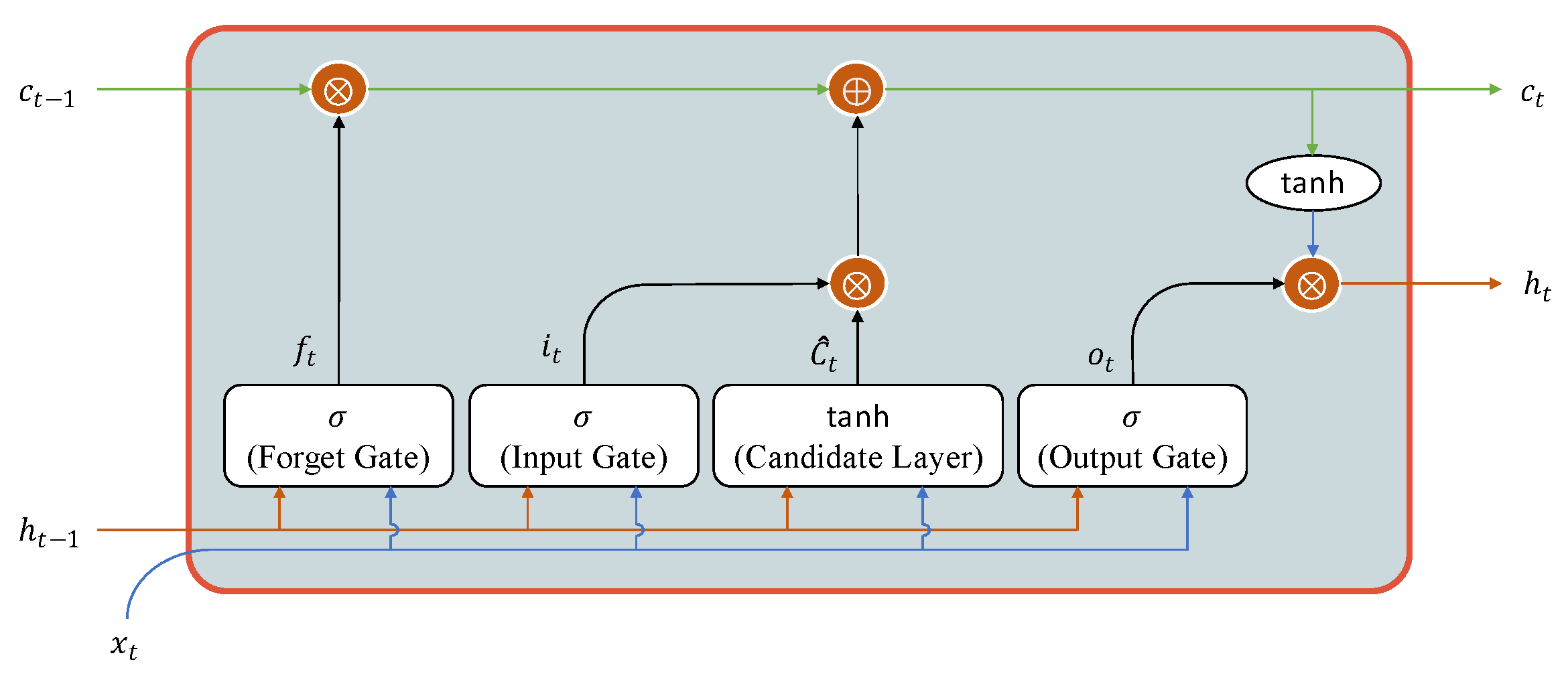
Figure 2.
Proposed LSTM-based train dynamic model: (a) the training phase; (b) the evaluation phase.
Figure 2.
Proposed LSTM-based train dynamic model: (a) the training phase; (b) the evaluation phase.
| Name of Types | Quantity |
| Hidden size | 64 |
| Number of LSTM layers | 2 |
| Dropout rate | 0.3 |
| Learning rate | 0.001 |
| Batch size | 128 |
| Number of epochs | 500 |
| Number of patience epochs | 30 |
Figure 3.
Comparison of the loss during the training stage.
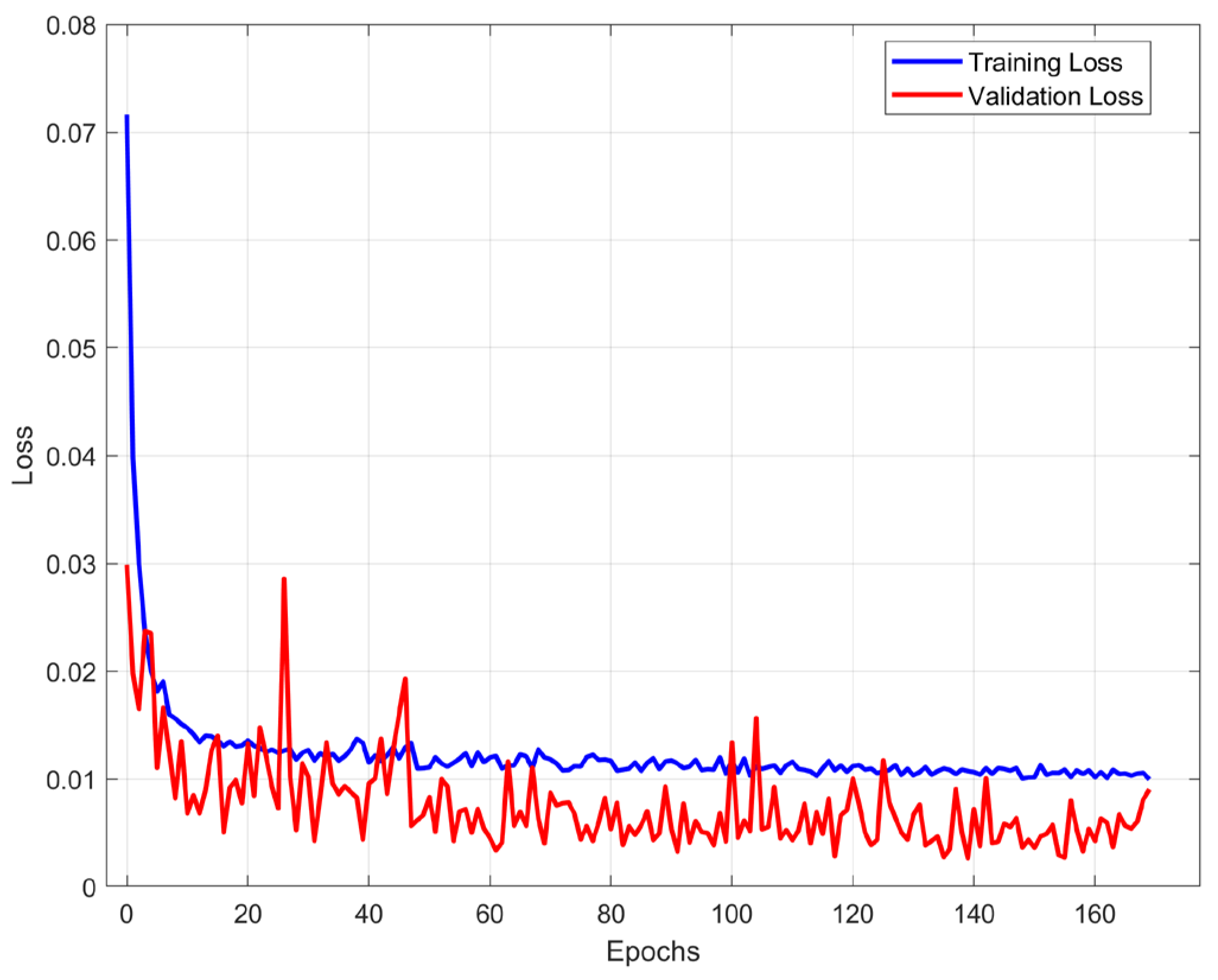
Figure 4.
Comparison of actual data and predicted train acceleration for stations by stations: (a) Stations 1 and 2; (b) Stations 3 and 4.
Figure 4.
Comparison of actual data and predicted train acceleration for stations by stations: (a) Stations 1 and 2; (b) Stations 3 and 4.
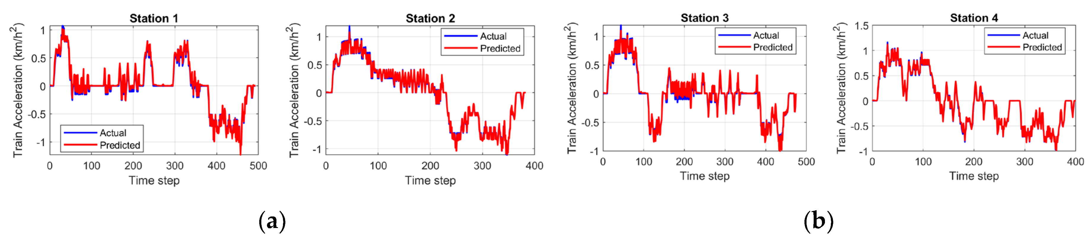
Figure 5.
Comparison of actual data and predicted train acceleration for stations by stations: (a) Stations 5 and 6; (b) Stations 7 and 8.
Figure 5.
Comparison of actual data and predicted train acceleration for stations by stations: (a) Stations 5 and 6; (b) Stations 7 and 8.
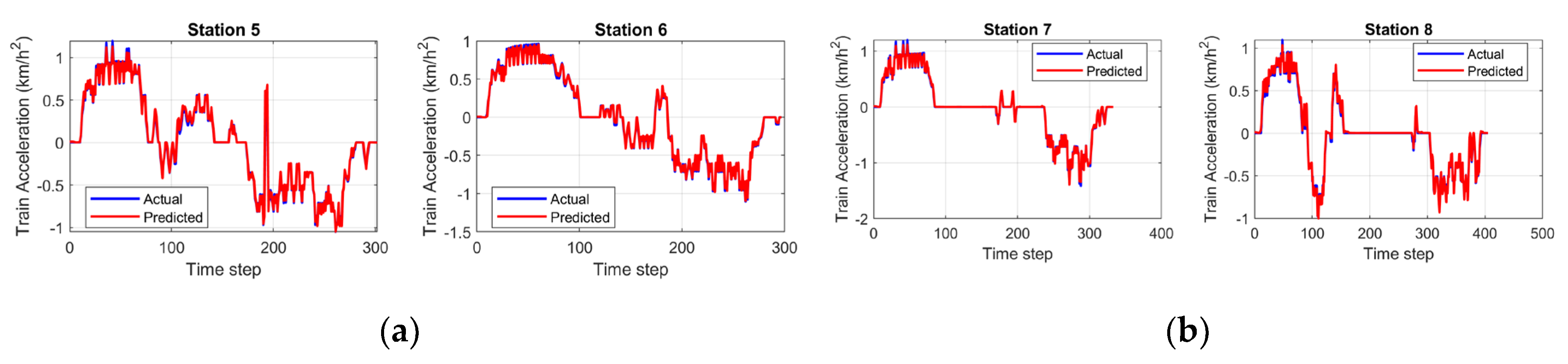
Figure 6.
Comparison of actual data and predicted train acceleration for stations by stations: (a) Stations 9 and 10; (b) Stations 11 and 12.
Figure 6.
Comparison of actual data and predicted train acceleration for stations by stations: (a) Stations 9 and 10; (b) Stations 11 and 12.
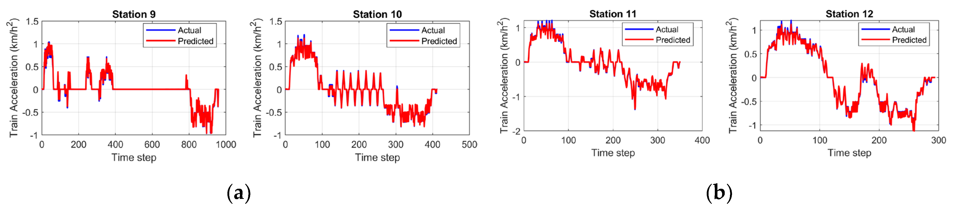
Figure 7.
Comparison of actual data and predicted train acceleration for stations by stations: (a) Stations 13 and 14; (b) Stations 15 and 16.
Figure 7.
Comparison of actual data and predicted train acceleration for stations by stations: (a) Stations 13 and 14; (b) Stations 15 and 16.
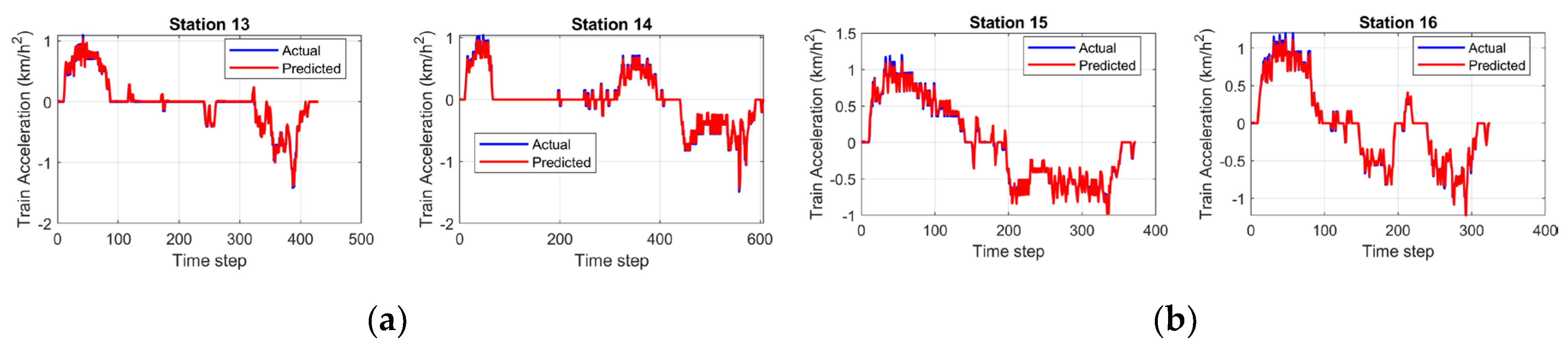
Table 2.
Performance metrics across all 16 track sections.
| Track Section No. | MAE | RMSE | R2 |
Mean Error |
Standard Deviation Error |
Minimum Error |
Maximum Error |
Percentile 95th Abs Error |
| 1 | 0.0223 | 0.0291 | 0.9952 | 0.0167 | 0.0238 | -0.0628 | 0.0851 | 0.0563 |
| 2 | 0.0128 | 0.0180 | 0.9989 | 0.0006 | 0.0180 | -0.1103 | 0.0587 | 0.0374 |
| 3 | 0.0221 | 0.0289 | 0.9953 | 0.0151 | 0.0247 | -0.0925 | 0.0793 | 0.0578 |
| 4 | 0.0107 | 0.0154 | 0.9990 | 0.0058 | 0.0142 | -0.0602 | 0.0630 | 0.0336 |
| 5 | 0.0142 | 0.0273 | 0.9974 | 0.0046 | 0.0270 | -0.0967 | 0.2702 | 0.0425 |
| 6 | 0.0102 | 0.0143 | 0.9993 | 0.0030 | 0.0140 | -0.0557 | 0.0429 | 0.0323 |
| 7 | 0.0108 | 0.0181 | 0.9989 | 0.0021 | 0.0180 | -0.0846 | 0.0752 | 0.0379 |
| 8 | 0.0144 | 0.0211 | 0.9976 | 0.0092 | 0.0190 | -0.0616 | 0.0724 | 0.0454 |
| 9 | 0.0083 | 0.0162 | 0.9972 | 0.0065 | 0.0149 | -0.0437 | 0.0824 | 0.0410 |
| 10 | 0.0113 | 0.0167 | 0.9987 | -0.0007 | 0.0168 | -0.0799 | 0.0459 | 0.0371 |
| 11 | 0.0150 | 0.0221 | 0.9984 | -0.0003 | 0.0222 | -0.0995 | 0.0598 | 0.0445 |
| 12 | 0.0139 | 0.0190 | 0.9990 | -0.0008 | 0.0190 | -0.0816 | 0.0491 | 0.0384 |
| 13 | 0.0103 | 0.0162 | 0.9984 | 0.0057 | 0.0152 | -0.1134 | 0.0576 | 0.0351 |
| 14 | 0.0111 | 0.0188 | 0.9977 | -0.0039 | 0.0184 | -0.0834 | 0.1567 | 0.0403 |
| 15 | 0.0138 | 0.0199 | 0.9987 | 0.0016 | 0.0199 | -0.0927 | 0.0652 | 0.0392 |
| 16 | 0.0128 | 0.0202 | 0.9986 | -0.0020 | 0.0201 | -0.0890 | 0.0450 | 0.0445 |
Table 3.
Summary of regression evaluation metrics across all 16 track sections.
| Regression evaluation metrics | MAE | RMSE | R2 |
| Mean | 0.0134 | 0.0201 | 0.9980 |
| Standard Deviation | 0.0039 | 0.0047 | 0.0013 |
| Minimum | 0.0083 | 0.0143 | 0.9952 |
| Maximum | 0.0223 | 0.0291 | 0.9993 |
Disclaimer/Publisher’s Note: The statements, opinions and data contained in all publications are solely those of the individual author(s) and contributor(s) and not of MDPI and/or the editor(s). MDPI and/or the editor(s) disclaim responsibility for any injury to people or property resulting from any ideas, methods, instructions or products referred to in the content. |
© 2025 by the authors. Licensee MDPI, Basel, Switzerland. This article is an open access article distributed under the terms and conditions of the Creative Commons Attribution (CC BY) license (http://creativecommons.org/licenses/by/4.0/).
Copyright: This open access article is published under a Creative Commons CC BY 4.0 license, which permit the free download, distribution, and reuse, provided that the author and preprint are cited in any reuse.


