
Submitted:
16 October 2025
Posted:
20 October 2025
You are already at the latest version
Abstract
We survey the idea that the particle/field duality can be promptly visualized using the LAN structure of modern computer networks, as the LAN seems point-like from outside (one point of contact with the internet, one public IP address), but its expansive nature affects its interactions (i.e., signal exchanges) with other LANs. The central premise is thus to consider all elementary particles (including empty space and the constituents of Dark Energy and Dark Matter) as being networks of nodes – termed átmita. In this work, some fundamental properties of átmita and their communication protocol are outlined. Utilizing this protocol, it is shown that placing LANs of átmita on the lattice of space generates defects, which increase the effective distance between points lying on opposite sides of them. It is explicitly shown that the Schwarzschild metric is valid around a spherical mass, as these diffusion-driven space-defects generate an effective curvature. Additionally, placing any LAN system in empty space generates three fully symmetric, mutually non-interacting versions of each particle type, termed X- Y- and Z-bases. Two of them (arbitrarily X and Y), are argued to be Dark Energy (DE), with all particles of Regular Matter (RM) and Dark Matter (DM) belonging to the third base. This would make DE Quintessence-like, but there are no distinct DE particle types to be found, each of the two DE bases has its own copy of all Standard Model and DM particle types. The three bases’ symmetry at the limit of low redshifts leads to ΩDE(t→∞)=0.66¯ and Ωm=0.33¯, in excellent agreement with the values reported by the Dark Energy Survey (Ωm=0.333−0.016+0.015) and by Pantheon+ (Ωm=0.334±0.018). Based on the above fully symmetric model for DE, Z-based particles are suggested to be able to tunnel through a (Z-based) barrier by turning for a short time to one of their two DE counterparts (either X or Y). By symmetry, DE particles tunneling would be turning (half of the time) to their counterparts of regular matter. These tunneling DE constituents are suggested to be vacuum fluctuations. It is argued that this could provide an explanation for the Vacuum Catastrophe and offer a prediction for the vacuum energy density: Its particle density should be equal to that of all RM and DM particles tunneling at any given moment. Subsequently, one can place a LAN of átmita inside another LAN, rather than in empty space. DM particles are argued to be comprised of X- or Y-based LANs inside a Z-based LAN, whereas RM particles to be Z-based LANs inside a Z substrate. Since both DM and RM particles have Z-based substrates, it is shown that they can interact gravitationally. Based on their (a)symmetry, the percentage of DM is found to be 80% of Ωm, i.e., Ωc=0.26¯, in agreement with the value reported by Planck Collaboration (Ωc=0.264±0.011). Finally, we survey the structure of all Zz particle types. Each one is identified to correspond to a known (first generation) particle of the Standard Model. Their basic characteristics are studied, in terms of charge, spin, possession of mass, stability, etc. It is predicted that neutrinos are Dirac, not Majorana particles and that the W± bosons, but not Z0, might be able to interact with DM particles, possibly offering an explanation for the recent anomalous measurement of their masses. Also, each Force (except for the Strong) is associated with a specific LAN surface and their strength hierarchy is suggested to stem from the relevant hierarchy of the distances of these surfaces from the particle’s router.
Keywords:
Particle-Field Duality
; Local Area Network
; Discrete space
; Dark Energy
; Dark Matter
; Quantum Tunneling
; Vacuum Fluctuations
; Standard Model Particles
1. Introduction
In the heart of quantum mechanics (QM) lies a series of “paradoxes”, which are fully described mathematically and surveyed experimentally, but nonetheless contradict common sense. These include (amongst others) the particle/field duality, which allows point-like entities to have field-like characteristics, as well as the notion that the spin of elementary particles is a type of angular momentum, even though the idea of the rotation of a point-like entity is nonsensical (i.e., it requires an infinite velocity).
This is not to say that elementary particles do not have both particle and wave characteristics, but rather to stress that these effects contradict common sense in the context of the current formalism of QM. Many interpretations of QM exist, such as the Copenhagen [1], De Broglie–Bohm [2] and the Many Worlds [3], but a comprehensive, intuitive picture of these phenomena is to some extend still absent. It is thus possible that to understand the aforementioned paradoxes in an intuitively comprehensive manner, one might have to move away from conventional pictures such as “particles” or “fields” whatsoever and find another mental frame that is better suited for the task at hand.
Indeed, during the past few decades several theories tried to do just that, such as String/M-theory [4] and Loop Quantum Gravity [5]. Another theoretical approach that closely aligns with the perspective developed in this study is rooted in Quantum Information. This branch of theories suggests that spacetime may not be fundamental but rather an emergent phenomenon arising from more basic quantum informational principles—such as the quantum bit (qubit) or the act of quantum measurement [6,7,8].
Here we will argue that the quantum properties such as spin should also be treated as emerging and that another mental frame, namely the local area network (LAN), might allow us to visualize a particle/field entity and its spin, without violating common sense [9]. In more detail, here we will utilize the notion of the LAN (from the field of computer networks) to draw images that have the seemingly paradoxical characteristics of the particle/field entity, while they relate to our everyday experience with these networks (Section 2.1-Section 2.2).
Further, we will follow this analogy and demand that all particles are networks of communication nodes, called “átmita”. Each átmiton would have its individual “address” (similar to the notion of the IP address of computers in a LAN) and in this context each particle would exchange information with its counterparts through empty space via a single communication node, termed the “router”, utilizing a single communication protocol that defines the signal exchange method. What we perceive as space would be the equivalent of the Internet (see Figure 1a and Section 2.1) and what we perceive as time would be the multiples of the elementary step with which the network topology changes.
The advantage of this construct is that it requires only one species of “nodes” and one communication protocol, from which one would, in principle, derive the fundamental properties of empty space, as well as the characteristics of the elementary particles and their interactions (e.g., charges, masses, symmetries, etc).
In this work, we will first outline the basic properties of átmita and their interaction protocol, noting, when appropriate, possible alternative versions of them (Section 3). Based on this model, a number of important results, notions and suggestions will be extracted, all stemming from answering the most fundamental question: How can we place a LAN of átmita in Space? This question has two parts: 1) How is the LAN connected to Space? and 2) What addresses will the átmita of a particle/LAN occupy? In a sense, question (1) asks us to draw a picture like Figure 1(a), while question (2) seeks to describe a picture like Figure 1(b).
Turning to the first part of the question, note that it is not straightforward, as Space will be axiomatically assumed to have the topology of a perfect simple-cubic crystal (i.e., with no intrinsic holes and defects, see Section 3) and only integer addresses (i.e., lattice points) are valid, so we can seemingly place the LAN’s router neither at a substitutional nor at an interstitial position.
By overcoming this impasse, it will be shown that placing a particle/LAN entity in Space creates an effective curvature, as each particle acts as a “defect” on the lattice of Space (Section 4.1), much like a crystalline defect in a condensed matter system. Following this notion, it will be argued that massive objects generate great amounts of such space-defects, due to all their internal interactions. These defects then diffuse in all directions by means of a random walk, with their net flow driven by a concentration gradient.
This mechanism will be suggested to be equivalent to the mass-generated curvature of general relativity (GR) [10]. Indeed, the equivalency of the defect-diffusion effect and GR’s curvature notion will be demonstrated for the specific case of a spherical mass, as the Schwarzschild metric [11] will be shown to be valid in the mass’ vicinity. Note, however, that GR is not linear and thus the general (in)compatibility of the two theories needs to be rigorously proven in another publication.
This result could be rather important, as – to the author’s best knowledge – this is the first time the Schwarzschild metric is reproduced in the context of discrete space and time. Moreover, this approach can be thought as complementary to other recent works, which indicate that topological defects (singularities) placed in empty space would give rise to a 1/r attractive force [12,13].
Turning now to the second part of the aforementioned question: To fully understand the implications of placing a LAN in Space, the addresses occupied by the LAN’s átmita also need to be defined. Resolving this issue requires an additional concept – that átmita have a finite internal memory – which has important consequences:
First, if each átmiton has a finite internal memory of size M, then it can be argued that LANs of átmita exhibit the quantum mechanical wave-like characteristics. Indeed, in Section 3.3 we will suggest that De Broglie’s formula is valid in this context, by demanding that M is Plank’s constant h translated to the natural units of Átmiton theory.
Second, in Section 4.2 it will be detailed that, due to the átmita’s finite memory, the act of placing a LAN in Space results in three fully symmetric and non-interacting versions of each particle type – termed X- Y- and Z-bases. It will be argued that two of these bases correspond to Dark Energy (DE) and the third (arbitrarily chosen to be the Z-basis) to matter (both regular and dark varieties). In other words, according to this work there are two fully symmetric and mutually non-interacting versions of the electron, and , in addition to the regular electrons (i.e., ). The same also holds for all other particle types.
This model can be used to calculate the percentage of DE (at the limit of low redshifts) to be , in excellent agreement with recent observations (see Table 1). Note that this is a Quintessence-like model for Dark Energy [14,15,16,17,18], not a cosmological constant. Recent findings [19], that suggest a non-zero cosmic birefringence angle in the Plank 2018 [20] data (albeit not yet with a 5 significance), as well as a coupling between supermassive black holes and DE [21], further support this view.
Furthermore, the above model for DE offers another interesting possibility: Since the three bases (X- Y- and Z) are fully symmetrical, it is conceivable for the router átmiton of a Z-based particle to be able to temporarily rotate by 90° its local (internal) coordinate frame and turn the particle (for a short period) to one of its X- or Y-based counterparts (Section 4.3). This way it can bypass a Z-based obstacle, with which it will not be interacting for the duration of its transformation to DE. The particle could now propagate through the Z-based barrier and resurface as a regular matter particle on the other side. This proposed mechanism sounds very familiar: It has the qualitative characteristics of QM tunneling.
However, if this is the case, then by symmetry DE particles should be able to tunnel by turning to their counterparts of the other two bases, i.e., by turning to regular matter with a 50% probability. Such tunneling DE particles would be (for the duration of the process) completely indistinguishable from their regular-matter counterparts, but from the point of view of a regular-matter observer they would appear out-of-nowhere and disappear as suddenly. Again, this possibility sounds very much like a known phenomenon, that of vacuum fluctuations.
This dual mechanism for tunneling and vacuum fluctuations could potentially explain the Vacuum Catastrophe and also provide a prediction for the vacuum particle density, as it should be equal to the flux of regular and Dark Matter particles tunneling at a given moment. Additionally, based on this model for DE, it seems that no distinct Dark Energy particle types are to be found, but rather we have already encountered (tunneling) DE particles as components of the vacuum fluctuations.
Third, in Section 2.2 it will be suggested that placing a LAN inside another LAN might allow for an intuitive picture for the particle’s spin (see Figure 2). Following this idea, we will construct all possible second order systems (i.e. systems of LANs with embedded LANs in them) and we will survey their characteristics. In Section 4.4 it will be shown that placing the internal LAN inside a Z-based substrate results in three different types of systems, noted as , and (utilizing the exact same mechanism used to define Dark Energy, vide supra). and will be collectively suggested to be Dark Matter (DM) and Regular Matter (RM).
Due to the finite memory of átmita, these flavors of matter do not interact with each other, except through their common Z-substrates, i.e., only gravitationally. Because of the symmetry break between and the (fully symmetric) and types, it is shown that the percentage of should be 20% of Z-based matter. This leads to the percentage of DM to be , in good agreement with observations (see Table 1).
Fourth, in Section 5 we will survey the properties of all possible second-order structures. There are sixteen distinct systems, each of which will be corresponded with a (first-generation) particle of the Standard Model. Based on the structure of each system, some fundamental properties of each particle type will be discussed, such as how spin, mass, stability, charge conjugate symmetry and EM charge arise in each case. The systems that correspond to the graviton, the photon, the electron and the boson will be surveyed in more detail and their specific properties will be extracted, albeit qualitatively. In this context, spin will be argued to arise from a periodic motion of the internal LAN(s) inside the substrate (similarly to Figure 2) and mass from the motion of the internal LAN parallel to the momentum of the particle (i.e., from a longitudinal component of spin).
Although in this publication the neutrinos are not studied in detail, it will be evident by their structure that they are Dirac, not Majorana particles [32]. Also, the fractional charges and colors of quarks, as well as the charge of the W-bosons, will be argued that it might be related to internal tunneling, i.e., of a periodic transformation of one of the internal LANs of the particle to one of the two Dark Matter counterparts. Such a mechanism should be absent in other particles (e.g., the boson), which might provide an explanation for the anomalous mass measurement of the W-bosons [33,34,35,36], as it would allow these charged bosons to interact with Dark Matter particles.
Finally, in the Supplementary Information recipes for how to get Electromagnetism, the Weak force and Gravity out of the single communication protocol of átmita will be discussed, by correlating each Force with a signal coming from a surface of one of the particle’s LANs. Based on these (qualitative) recipes, several of these Forces’ known properties will be derived and the hierarchy of their relative strengths will be discussed in terms of how far away these surfaces lie from the particle’s router.
From the above outline of Átmiton theory, it is evident that this study will be introducing a plethora of new concepts, which need to be properly defined and explained. This is done primarily in the Supplementary Information via figures and examples, but also in the later sections of the main document (Section 4, Section 5 and Section 6). In those sections, all these novel concepts will be anchored to known attributes and phenomena of CDM and the Standard Model, which will hopefully aid with their comprehension.
As this is the first publication on Átmiton theory, several results will be shown in detail, but there will also be a lot of suggestions and notions that should be further surveyed with subsequent studies. These should be considered as hits for further avenues of development, rather than claims to extraordinary results set in stone.
2. Using the LAN Structure to Visualize Quantum Paradoxes
2.1. Visualizing a Particle/Field Entity
In computer networks, the local area network (LAN) refers to a communication network of nodes (typically computers, smartphones, etc) that are interconnected through a network topology (meaning the map of the nodes’ connections) and are able to exchange information. Information exchange between two nodes in the same LAN makes use of a single identification number for each node, called the private IP address (IP stands for “Internet Protocol”), assigned to them by a special node, called the router. The private IP address is locally unique, in the sense that no two nodes in the same LAN can have the same private IP, but nothing prohibits nodes belonging to different LANs to share a private IP.
If a node in a LAN wants to connect with a node outside the local network (e.g., with a computer in another LAN), it can do so through a router that is connected with the Internet, which is a network of networks. To communicate through the Internet, all nodes in the same LAN share the same, single identification number, called the public IP address, and send messages to the outside world with the router acting as the sole gateway. The public IP address of each LAN is thus globally unique and in an abstract way defines the position of the LAN’s router on the global network.
Based on the above, if one depicts the topology of the interconnections of all nodes on the Internet based on their (public) IP addresses, each LAN would look point-like, in the sense that all of its nodes have the same public IP address and the LAN has a single point of contact with the Internet (see Figure ??). On the other hand, the fact that the LAN has actually some internal structure makes a large difference in regard to the way it interacts with the rest of the world, as a LAN consisting of a single node would create, process and demand data in a completely different way than a LAN consisting of hundreds of telecommunication nodes interconnected with a certain network topology (compare LAN1 and LAN2 in Figure ??).
Furthermore, given that the private IP addresses of the nodes in each LAN are only locally unique, there could be nodes in other LANs with the same IP addresses. As a result, if we imagine an abstract “address-space” of IP addresses, in which each node of every LAN is placed according to its local address, then each LAN would cover a portion in this space (i.e., a field), with several LANs potentially overlapping each other, just like fundamental physical fields overlap at each position of space in quantum field theory.
The above considerations allow us to draw an interesting parallel to Particle Physics, by noting the Internet as analogous to space, the router connecting each LAN to the Internet as analogous to an elementary particle’s position and each particle’s field analogous to a LAN, sharing with other LAN/particles potentially overlapping portions of an abstract address-space hovering over space. In other words, it seems that a LAN can be thought as having both point-like and field characteristics, in analogy to an elementary particle in quantum (field) theory.
2.2. Visualizing the Spin of a Point-like Entity
Let us now embed a new LAN inside the initial LAN. The initial LAN (acting as a substrate for the new LAN) would then be external, in the sense that has a direct connection with the Internet, whereas the new LAN would be internal, as it has no direct connections with the Internet (Figure 2). The internal LAN would seem point-like to an observer being at some node of the external LAN, while an observer outside both LANs (i.e., on the Internet) would deem the whole structure as being point-like.
Indeed, LAN3 in Figure 2 consists of an internal and an external LAN (termed I-LAN3 and S-LAN3, accordingly), but for an outside observer the collective LAN3 would still look point-like and identical to LAN1 of Figure 1(a). Nonetheless, LAN1 and LAN3 have different internal structures, which could cause them to exhibit very different characteristics.
For instance, if we now allow I-LAN3 to be hopping around S-LAN3 by gradually shifting its router’s connection from one node of the substrate to the next in a circular manner with a characteristic period (see Figure 2), then this motion can be considered (after appropriate definitions) to be carrying spin (i.e., intrinsic angular momentum). Note that the rotation of I-LAN3 is (the analogous of) a motion on a field (i.e., the substrate S-LAN3) and not in space (i.e., the Internet).
For an observer on the Internet, this spin would have no physical meaning, as they would perceive the whole structure of the two nested LANs as a single point, incapable of having internal motions/rotations, but at the same time, this spin would manifest itself through the interactions of the nested system with other LANs, as the time it takes for a signal coming from outside LAN3 to arrive to a specific node of I-LAN3 would depend on the distance between the routers of the internal and the substrate LANs, which would be fluctuating due to this periodic motion.
As an example, in the situation depicted in Figure 3 the signal going from node of I-LAN3 to node of LAN2 would have to cross the static number of nodes on the Internet separating the routers of LAN3 and LAN2, plus a fluctuating number of internal nodes, namely: , where is the total number of intermediate nodes that this signal has to cross in its route from to , is the number of nodes on the Internet separating the routers of LAN3 and LAN2, is the number of internal nodes separating the router of I-LAN3 and S-LAN3 and similarly for .
An outside observer would still consider both LAN3 and LAN2 to be point-like (like Figure 1(a)), thus they would consider only as the distance of the two point-like particles, whereas they would be oblivious to the fluctuating and internal distances.
In the hypothetical scenario that there is a law connecting the strength of the interaction of I-LAN3 and LAN2 with the total distance separating nodes and , then this law would have two separate terms: One term that would only depend on the distance of the two LANs’ router on the Internet and another term that would depend on the phase difference of the two systems’ internal rotations.
This, of course, is qualitatively in line with the usual QM situation of breaking the wavefunctions into independent spatial and spin terms, the former depending only on the distance between the two particles in space and the latter on the two particles’ phase difference at a given point in time.
2.3. Roadmap for the Development of Átmiton Theory
The aforementioned analogy between LANs and quantum particles is arguably useful by itself, as it can enhance our intuition on these quantum paradoxes. But it also allows for the enticing possibility that the LAN/particle analogy might actually stem from a deeper connection between these two structures. We will thus argue for the need of surveying the possibility of a new formalism for quantum and particle physics, having the notion of the LAN at its heart.
This formalism, which we will term as “Átmiton theory”, would have all elementary particles being (systems of) LANs, each type of particle (e.g., , , etc) exhibiting its unique characteristics by having a discrete network topology. These LANs/particles would then interact with each other by exchanging signals that propagate through space (which would thus play a role analogous to the Internet). On the one hand, this analogy provides a mental picture of how an expansive entity – like a field or a wave – can appear point-like from outside. On the other hand, accepting the aforementioned premise immediately leads to several important notions:
1) The position of an elementary particle would correspond to where the LAN’s router is connected with the Internet/space.
2) Space would be discrete in this setting and space would be made of the same type of nodes as any particle. We will be calling these nodes átmita. Note that if all particles are made of the same underlying “essence” as space, this could further demystify the known phenomenon of the Cosmic Background Radiation losing energy as the Universe expanses [20,37], given that the átmita that form the expanding space would have to come from an equal amount lost by particles.
3) Another important consideration for this model is the definition of time. If we allow all nodes to be switching positions with one of their nearest neighbors in every LAN once per unit time (like the router of I-LAN3 in Figure 2), then this hop rate would define the highest possible speed (i.e., the speed of light) and each such “turn” the quantum of time, but it would impose no upper speed boundary for information propagation. This instantaneous information exchange could allow for two LANs to share a virtual connection over large distances, possibly providing a mechanism for two far-away particles to form an Einstein–Podolsky–Rosen (EPR) connection [38,39].
4) Since all nodes inside the LAN are not directly connected with the Internet/space, they would have to send their signals to the outside world through the router, which would translate them in a form that can propagate in space (i.e., through a process similar to translating the private IPs to a public IP address, organize how the signal will be transported on the web, etc). Systematic differences on how these signals are structured (due to different network topologies of different kinds of particles) might potentially explain how the different characteristics of the Physical Forces (Gravity, EM, etc) could arise from a single communication protocol.
5) Effectively, each LAN would correspond to a field, with each particle potentially consisting of a number of fields, either embedded in each other, or possibly placed on a common substrate LAN. Particles having distinctly different systems of LANs, would thus exhibit distinct attributes in terms of these fields (i.e., maybe the graviton would consist only of the “gravitational” LAN, whereas the photon would also have LANs relevant to EM and the Weak Forces).
6) In Particle Physics, the Fields that give rise to Gravity, EM and the Nuclear Forces are considered completely separate from each other (unless they are explicitly coupled via some interaction [40]). This leads to the many independent parameters of the Standard Model, which can be fine-tuned in isolation. But the idea presented in Section 2.2 that placing a field inside another field could generate the particle’s spin, might reveal a deeper connection of these fields (if, say, the substrate LAN was the Gravitational Field, the internal LAN the EM Field, etc). If such deeper connections indeed exist, then such a formalism might be able to reduce the number of free parameters of the (equivalent of the) Standard Model.
We conclude that a major advantage of such a formalism is that it would require only one species of “nodes” and one communication protocol, from which one would, in principle, derive the fundamental properties of elementary particles (e.g., charges, masses, symmetries, etc) and their interactions (all based on their network topology).
To realize these notions and survey some of their consequences we need, therefore, to formulate a model that can fully replace the particle/field entity with systems of LANs. Here, we will start this discussion by outlining the roadmap of the creation of such a model and the main questions that need to be answered during its development, which will then start addressing in Section 3 and in the Supplementary Information.
First, one would need to define the basic attributes of the fundamental entity of this framework, namely the node-like entity that we will be calling “átmiton”. At the very least, the átmiton should be able to form connections with other átmita (in order to construct LANs) and exchange information via signals.
Already we can identify several issues that need to be addressed. Regarding the way átmita are interconnected, one needs to answer questions such as:
- How many nearest neighbors can an átmiton have?
- What is the dimensionality of their network (e.g., is the network 2D, 3D, etc)?
- What is the “crystal structure” – the local topology – of the network (i.e., is the network’s symmetry in line with a simple-cubic lattice, or some more complicated structure)?
- How do átmita move on the network? Is their move instantaneous, or does it happen in steps?
- How big is an átmiton? Is its size on the order of the Plank length?
Also, regarding the way átmita exchange information, one needs to define their “Communication Protocol”, which would at least provide answers to questions such as:
- What kind of information does each signal contain?
- How can the receiver identify the sender of the signal? In other words, is there some sort of unique identifier, or “address”, for each átmiton?
- If átmita have a well-defined address, then is this address globally unique (like the public IP address of communication nodes), or is it a locally defined property? If the latter, then how are addresses translated from one “frame” to the other?
- How does each signal propagate on the network? E.g., is it broadcasted? How does it move from one node to the next?
- What effect would a given signal have when it reaches a certain (receiving) átmiton?
With a set of axioms and protocol processes that cover (at least) the above considerations, we will then start forming LANs of átmita and place them either in space, or on substrate LANs. To do this, as mentioned in Section 1, we need to understand: (1) How is the LAN connected to space (or to its substrate LAN)? Is there a “router” átmiton connecting the LAN with space? If yes, what is its functionality? and (2) What addresses will the átmita of a particle/LAN occupy (i.e., is there a process similar of the one translating a private IP address – which is only locally unique – into a – globally unique – public IP address)?
Clearly, the approach outlined above moves from the bottom up, i.e., from individual átmita →LANs→particles with unique topologies→ derivation of their symmetries and characteristics. In principle, therefore, the collection of axioms and protocols that cover the aforementioned basic characteristics of the átmiton and its interactions should be the only ad hoc ingredients of the theory, everything else (e.g., particle symmetries, charges, characteristics of all physical Forces, etc) should get derived from these fundamental statements. Note that even though these statements will naturally be carrying some degree of arbitrariness (as is true for the foundations of every theory), this will be of a discrete nature, since – for example – the number of an átmiton’s nearest neighbors cannot be fine-tuned in the same way as the coupling constants of the Standard Model; that number should at least be a (relatively small) positive integer, directly connected to the local topology of the network.
3. Basic Principles of Átmiton Theory
In the spirit of the ideas mentioned in the previous sections, we demand an entity with no internal structure, called átmiton, that can form a network with other átmita by exchanging information that establish connections. Átmiton is the only ingredient of this theory, in the sense that everything else (i.e., empty space, particles/fields, etc) will be considered to be systems of interacting átmita, with their network topology being what gives rise to the different characteristics of these systems (see Section 4-Section 5).
In its essence, an átmiton resembles a telecommunication node, or a simple computer on a network. It interacts with the other átmita on the network by sending signals that propagate through the network in an instantaneous but causal manner, in the sense that the signals will have to pass through each intermediate átmiton to arrive to their destination, similarly to how in chess a bishop can move through multiple cells in a single move (instantaneous), but only if each one of the intermediate cells on his path is unoccupied (causal).
Here in the main manuscript we will give a relatively brief outline of the basic properties of átmita, but for a more thorough discussion see the Supplementary Information (Section ??). A summary of this discussion is condensed in Supplementary Section ??.
3.1. Átmiton’s Connections and Address
Fundamentally, each átmiton should be able to form connections with other átmita in order to create a LAN; similarly to how the nodes of Figure 1 and Figure 2 are connected. The number of possible direct connections an átmiton can have (i.e., the number of its so-called ports, each port capable of connecting with a neighbor) is therefore the most basic attribute of these entities. It is defined axiomatically to be six: Two neighbors at each dimension of a 3D network. In other words, the “crystal structure” of the network is that of the simple cubic crystal (see Axiom 1 in the Supplementary Information).
Of course, átmita should be able to interact with non-nearest neighbors, which is accomplished by passing the relevant signals from one direct connection to the next, similarly to how computers exchange information online. A very useful metric of that interaction is, therefore, the connection distance, , of those two átmita (denoted as A and B): It is defined to be the number of direct connections in the shortest continuous path that enables them to interact. Evidently, the connection distance of two nearest neighbors defines the quantum of distance in this theory, which we will be calling stathmós (plural: stathmoi) and we will be denoting as in natural units or (i.e., quantum of length) in the International System of Units (SI).
From the above, it becomes immediately apparent that Space in this context is fundamentally static, flat and discrete (being a simple-cubic crystal). This seems to be at odds with both the curved spacetime continuum of general relativity and with the active vacuum soup of quantum field theory (QFT) [41,42]. Nonetheless, in Section 4.1 it will be demonstrated that particles introduce an effective curvature at the point they are connected to the lattice of Space (i.e., at their router), which makes a given distance in their presence seemingly longer. Also, in Section 4.3, we introduce the idea that vacuum energy comprises of Dark Energy particles tunneling by temporarily turning to their regular-matter counterparts and in Supplementary Section ?? we will show that DE creates an apparent expansion of a given distance (as seen by a regular-matter observer), in line with current astronomical observations. As a result of these effects, both the spacetime curvature of GR and the vacuum fluctuations of QFT can be thought of being superimposed on the above static background of Space átmita.
Turning now to the interaction of individual átmita, it is important to understand what sort of signals do the átmita exchange and to what effect. These questions are addressed by Axiom 2 and Protocol Process 1 in the Supplementary Information: As stated in Axiom 1, each átmiton has six ports, one for each possible nearest neighbor. According to Axiom 2, if a given átmiton, A, has fewer than six nearest neighbors (and thus has an open port), it will broadcast a signal to the network, containing the address of the hole (see átmiton A of Figure 4).
The effect of that signal is defined by Protocol 1: If another átmiton, B, receives the signal and has a relevant open port (e.g., A signals a [] hole and B haves a [] open port), then they will interact and potentially start moving on the lattice towards each other, until they annihilate their holes (see Supplementary Figure ??). Else, átmiton B will pass the signal sent by A along to the rest of its nearest neighbors. This is, in principle, the root of all interactions in this theory, whereby communicating átmita can converge and form a compound network (i.e., a unified LAN).
It is evident that the above signal exchange requires for each part of the interaction to have a unique identifier; like the “From/To” information needed to send an email. Thus, we demand (Axiom 3) that each átmiton should have a unique address that permits it to exchange information (in the form of signals) with other átmita.
An important point discussed in the Supplementary Information is that these addresses are unique when compared in the same frame of reference. Each átmiton has its local frame of reference, to which it translates all other addresses. In simple scenarios (such as the ones depicted in Supplementary Figure and Figure 4) this translation is trivial (i.e., neighboring átmita have “neighboring” addresses in all frames), but in more complicated instances this process can result in addresses of nearby átmita that are widely different from their position on the lattice (see Section 3.4).
Based on the above, the notion of an átmiton’s address leads to a second measure of distance between two átmita, namely that of the address distance, of two átmita with addresses expressed as the vectors p and q. When the address translation between the frames of the two átmita is trivial (e.g., Figure 4), then these two measures of distance ( and ) are equivalent. Nonetheless, in most cases of practical significance this is very much not the case, as will be discussed in Section 3.4. Indeed, in the context of this theory, the non-interactive nature of Dark Energy and Dark Matter (excluding gravity for the latter) stems from (see Section 4 and Supplementary Sections ??-??).
Therefore, it seems natural to bundle into a single entity all átmita that translate their addresses trivially from one local frame to all others’. This will be called a LAN, which is a collection of átmita that share an effective frame of reference, meaning that for each pair of átmita A and B in the LAN, the translation of their addresses to each other’s frame is trivial. The átmiton of a substrate (or Space) on which a LAN is connected will then be called router átmiton. The router can be thought of being a part of both the LAN and its substrate, as it has the role of translating the addresses from one effective frame of reference to the other (similarly to how the router translates the private IP addresses to public IP). Detailing this process will be the main focus of Section 3.4. The collection of LANs which are connected to Space through the same, single, router átmiton will be what we will call a particle. For example, the combination of the internal end external LANs (denoted collectively as LAN3) in Figure 2, would be considered a particle.
As an example of the above discussion, Figure 4 depicts a simple case with an átmiton, A, that has an open port and to close it, it generates and broadcasts a signal. Note how the signal is translated from the local coordinate frame of átmiton A: [](), to that of átmiton B: []().
Based on Protocol 1, such a signal exchange would ultimately lead to átmita moving on the lattice (see, e.g., Supplementary Figure ??). Axiom 4 and Protocol 2a define how this motion takes place on the lattice (Supplementary Section ??), by providing an answer to questions such as: How do interacting átmita move to converge? Is the move instantaneous (like the way their signals propagate on the lattice), or it happens gradually? With Axiom 4, we demand that the internal topology and the position of each LAN (relative to other LANs) evolves in turns, each of which is called a gyros (plural:gyroi) and is denoted as in natural units or in SI. Obviously, one gyros is the quantum of time in this context.
In turn, the specific way átmita move on the lattice is defined by Protocol Process 2a: During each gyros, each átmiton can hop to fill a vacant port of a nearby átmiton, by changing its address (in any given frame) by one unit (see Supplementary Figure ??). The allowed (by Protocol 2a) hop of one unit per gyros of an átmiton moving in its LAN, defines the maximum allowed speed in this theory and will be denoted as the speed of light.
A critical detail in Protocol 2a is that only movements to vacant ports on the lattice are allowed. This is a direct consequence of Axiom 3, as a movement to a filled position would result in two átmita sharing an address. Thus, in the situation depicted in Figure 4, átmiton A can hop to the vacant position at its left during the next gyros, but cannot go towards any other direction, as all of its other nearest neighbors’ ports are filled. In addition, due to the same reason, átmiton B of Figure 4 would not be able to move towards the vacant position at the left of A, even if B had a relevant open port.
As a final point, note that if the interaction between two átmita is intra-LAN, then each átmiton can move independently from the rest of its LAN towards the hole, as is the case for átmiton B in Supplementary Figure ??. But if the interaction is extra-LAN, then the whole LAN should move in address-space towards that hole. Therefore, this motion of the LAN in address-space requires an actual motion of the particle’s router in Space (or on its substrate more generally). This distinction will be utilized in Section 5 and in Supplementary Sections ??-??, in order to understand which interactions generate the internal characteristics of a particle (e.g., its spin, stability and mass) and which interactions generate the physical Forces felt by the particle through Space.
3.2. Memory of the átmiton
If the interaction of an átmiton is with some distant átmiton, how does it know what path to follow on the lattice to reach that open port? Also, can an átmiton interact with a signal coming from an arbitrarily large distance? Axiom 5 addresses these issues (Supplementary Section ??), by stating that each átmiton has a finite internal memory of size M, where M is a very large natural number. In this memory, the átmiton stores the information needed to reach (generally after several gyroi) the open port with which it interacts.
In Section 3.3, it will be argued that the finite memory of átmita might be at the root of the wave-like properties of particles. Indeed, in Section 3.3 the De Broglie formula will be recovered, by demanding that M is actually Plank’s constant h, translated to the natural units of this theory. Also, in Section 4.2-Section 4.4 we will utilize Axiom 5, in order to understand the lack of interactions between particles or regular matter and their counterparts of Dark Energy and Dark Matter.
The general way that information is stored in the átmiton’s memory is defined by Protocol Process 3a (see Supplementary Section ??): Let an átmiton A interacting (in the sense of Protocol 1) with an átmiton B, which lies at a connection distance and an address distance . Then, the memory volume that átmiton A reserves (in order to define the map of how to reach the open-port of átmiton B), consists of blocks of memory units, each block defining one gyros of the process and the total number of blocks being proportional to . The memory volume of each such fundamental block is a monotonically increasing function of .
We can note the above form for the memory map as , where (i.e., the memory block’s volume) is a monotonically increasing function of (see Supplementary Figure c,d).
Note that the above form of Protocol 3a is somewhat vague in terms of how the memory requirements of an interaction are organized in the átmiton’s memory. To be able to use the axioms and protocol processes governing the behavior of individual átmita in order to simulate/calculate quantitative properties of each elementary particle would require an updated version of Protocol 3a, with an explicit form for . Nonetheless, the above general model for is enough for deriving a number of important results, such as calculating ab initio the percentages of Dark Energy and Dark Matter, showing the cause of their (lack of) interactions with particles of regular matter (Section 4.2-Section 4.4) and demonstrate several important qualitative characteristics of the known Standard Model particles, such as their EM charges, spin and stability (Section 5).
For instance, a crucial result that stems directly from Protocol 3a is that two átmita that have an address distance , such that , would not interact regardless of how small their connection distance is (i.e., regardless of how close they are in Space), as the information defining the interaction would not fit in the átmiton’s memory ( would be out-of-bounds).
In Section 4.2 it will be suggested that this is why particles of regular matter do not interact with their Dark Energy counterparts, even if they are extremely close to each other in Space: Although their distance can be arbitrarily small, their address-distance is such that is always larger than M (this is explicitly shown in Supplementary Section ??).
From the above discussion is clear that for a given interaction between two átmita, there is a maximum connection distance for which . If the second átmiton is farther away than , the first átmiton won’t interact with it. The value of depends on the configuration of the two interacting átmita’s LANs. For instance, it can be vastly different if the two interacting átmita belong to the same LAN, or not, see Section 3.4. Indeed, given that a LAN has a single effective coordinate frame, which trivially translates its átmita’s addresses from one to the other (i.e., ), intra-LAN interactions should be the case with the maximum possible value of from any conceivable configuration (see cases studied in Supplementary Section ??). This ultimate will be denoted as .
Protocol 3a (discussed above) outlines the way an átmiton stores in its memory the information of one signal. But what if that átmiton has more than one open port and thus receives several corresponding signals? How will these signals be stored in its memory and how will they affect its future path on the lattice?
We require with Protocol Process 3b (see Supplementary Section ??), that the átmiton in question fills its memory gradually, by adding each memory map as they arrive to it, step by step: It will first put the information of the nearest signal () to its memory and (if there is still space in its memory), that of the second closest signal (), etc, until either all signals are registered in its memory, or its memory runs out of space.
Protocol 3b allows us to study extra-LAN interactions (i.e., interactions between átmita belonging to different LANs). These would result in the router átmiton R of the LAN to move in Space, in order for the interacting átmita to converge (see, e.g., Supplementary Section ??). But a LAN generally contains multiple átmita with open ports, at least on all of its surfaces. Hence, these can generally participate at the same time in several individual interactions, each with its own memory map. All the memory mappings of every átmiton of the LAN interacting with other LANs should be weighed by the router átmiton, which should translate these interactions to an actual motion of the particle in Space, by a series of hops (Protocol 2a). According to Protocol 3b, the nearest átmiton to the router R that participates in an interaction will send its memory map of volume and this map will be stored in the router’s memory (provided of course that ). If there is remaining space in its memory, the router will add , , etc, until it fills its memory completely.
From the above, it is evident that the closer an átmiton of the LAN is to the router, the better chance it has to affect the particle’s motion by having its interaction engraved in the router’s memory. Thus, if one can attribute specific átmita with open ports (e.g., one specific surface of the LAN) to a specific force (e.g., Gravity), then as a rule of thumb the farther the átmiton generating the interaction lies from the router of the particle, the weaker the interaction. In Section 5 and Supplementary Sections ??-??, we will argue that specific surfaces of each particle of the Standard Model act as the “charges” of EM, Gravity and the Weak Force and we will derive their strength hierarchy (albeit only qualitatively) based on these surfaces’ proximity to the particle’s router.
3.3. The Wave-like Properties of LANs
Let us now move from the level of the individual átmita to that of their LAN. At this higher level the router átmiton is of the greatest importance, as its memory matrix defines the actual path of the particle in Space, i.e., it translates all the individual átmita’s interactions to a motion in Space.
Based on Protocols 3a,b, the memory of a particle’s router will be organized in memory blocks of average size each defining the motion of the particle/LAN in Space for one gyros. is what we will call energy, E.
The minimum allowed energy of a LAN (denoted as in natural units and in SI) would then be due to a single átmiton interacting with an open port of one of its next-nearest neighbors. Based on Protocol 3a, .
According to Axiom 5, the átmiton stores in its memory the information of how to reach its destination after several gyroi. We will denote the number of gyroi that fit in the memory of the LAN’s router átmiton as the LAN’s period. By definition, the period T is equal to: , where the brackets indicate the integer quotient of the division.
From the definition of the LAN’s energy and period and their relationship to the router’s memory, we conclude that:
where E is the energy and T is the period of the LAN. Note that , if .
As a result of Eq. 1, the larger the energy of the particle, the smaller its period, or equivalently, the larger its frequency. This is De Broglie’s formula [43] , with the substitution: . To extract M in natural units (as a unitless natural number), we have to turn h in units of , or equivalently M in units of :
where and are the quanta of energy and time in the natural units of Átmiton theory, and are the corresponding quanta in SI units and the Plank energy. Here it is assumed that the quantum of time in SI units, , is equal to Plank time ().
The final result, therefore, is that M as a unitless natural number is the Plank energy (reduced by ) written in units of energy quanta. This makes sense: The largest energy a particle can have (Plank’s energy) corresponds to the shortest possible period (Plank’s time). In Átmiton theory, when the energy is the maximum permitted, then and that leads to the shortest permitted period of one gyros, as there is enough memory-space to define the trajectory of the particle only for the next gyros.
Based on the above discussion, we can outline the model for how an átmiton interacting with an open port of an átmiton of another LAN can move towards it and fill the said hole: Its LAN’s router will hop on its substrate from neighbor to neighbor, provided they have open ports (Protocol 2a) with the path taken predetermined from the beginning, for as many gyroi as they fit in the router’s memory (Protocol 3a), i.e., for one period. Thus, it seems that either the LAN interacts with its environment only once per period, when the memory of the router is vacant (Supplementary Figure c), or alternatively that every time a memory block is executed, it gets removed from the router’s memory to make way for another interaction’s memory block to take its place at the end of the memory’s queue (first-in-first-out, like Supplementary Figure d).
The wave characteristics of particles might be understood in light of these possibilities. For instance, consider the double-slit experiment: The fringes appear when the wavelength of the light is on the same order of magnitude as the distance between the slits. According to this view, this is because a photon with a much shorter wavelength wouldn’t interact with the second slit (it would be out-of-bounds of its memory), whereas a photon with a much greater wavelength (and hence a large period) would have its path predetermined for a time-period much larger than the time it takes to transverse the distance of the slits, so the interaction with the other slit would be statistically insignificant, i.e, its phase will be changing too slowly to form an interference pattern. Thus, although individual photons pass through just one slit, there is an interference pattern because each one can “sense” the second slit through its (absence of) signals.
This memory-model could also be relevant to understanding how the virtual particles (of QFT) are able to get absorbed with 100% probability: They get emitted by the particle only if there is a pre-calculated path leading them to the absorbing particle with the duration of the path being less than a period. Else, they are not emitted. But due to its router’s finite memory, the higher the energy carried by the virtual particle, the shorter its period in which it can pre-calculate its path leading from the emitting to the absorbing particle. Using Eq. 1, this means that (in natural units), or (in SI units).
In summary, in this section the fundamental properties of individual átmita were outlined (for a more rigorous treatment, see Supplementary Section ??). Based on these fundamental statements, in Section 3.4-Section 4.4 we will study the properties of LANs of átmita, but still without detailing their internal structure.
Indeed, treating each LAN as a black-box of unknown shape and internal structure is enough to derive several important results, such as recovering the Schwarzschild metric around a spherical mass, finding recipes for Dark Energy, Dark Matter, quantum tunneling and vacuum energy, as well as for calculating the universe’s percentages of Dark Energy and Dark Matter. The internal (i.e., field) structure of the particles of regular matter will be the focus of Section 5, in which we identify each particle of the Standard Model to be a second-order system of átmita that obeys a certain symmetry.
3.4. Placement of a LAN in Space
Having defined some of the most fundamental characteristics of individual átmita, their LANs and their interactions, we now turn to the very important question of how to place such an entity on the lattice of Space. Since Space is a vast 3D network of átmita with the simple cubic topology without holes and only integer addresses are valid (see Section 3.1 and Supplementary Section ??), the LAN’s router can be placed at neither an interstitial nor a substitutional position. Thus, placing a LAN in Space would require to either: (A) increase the dimensionality of Space by 1 (from 3D to 4D, hence increase according to Axiom 1 the number of possible direct connections for each átmiton by two), or (B) to (locally) re-define one of the three dimensions of the router átmiton’s coordinate system to point towards its connection with the LAN and not towards its nearest neighbors at one dimension of Space (see Figure 5).
To keep Space 3D, we will demand with Protocol 4 (see Section 3.5) that the router átmiton (denoted as R in Figure 5b) re-defines one of the x- y- or z-dimensions of its local coordinate system to coincide with the connection established with the LAN. Effectively, this coordinate-recalibration creates a field, i.e., a (kind of) space overlapping our regular Space.
Which dimension does the router choose to repurpose, in order to connect with the LAN? According to Protocol 2a, the LAN connected to router R can only hop to a neighboring átmiton of Space, if it has an open port. For example, for átmiton G of Figure 5b to move in address-space, its router R has to hop by swapping positions with one of its neighbors in the [] or [] directions, as all other nearest neighbors of R do not have open ports. Thus, the repurposed dimension defined by Protocol 4 is not fixed, rather is always parallel to the instantaneous motion of the particle in Space, as the introduction of the broken connections is what allows the motion of the router in Space in the first place.
This field-creation process is possibly the most critical aspect of the axiomatic formulation of this theory, as it governs everything, from the differences between DE, DM and regular matter particles, to several key characteristics of each particle type (Section 4- Section 5). In a sense, the rest of this publication from here on is just a discussion on the consequences of this process.
In more detail, therefore, a full comprehension of the situation depicted in Figure 5 requires a three-pronged approach:
(A) We need to define what address átmiton G of Figure 5b will occupy, without address-collisions with átmita of Space. This will be accomplished with Protocol 4, which is detailed in Supplementary Section ?? (and its consequences will be surveyed in Section 3.5).
(B) Since one dimension of R’s coordinate system is repurposed for connecting with the LAN, the two former connections of R with the neighboring Space átmita across some dimension will have to break (see the red connections of Figure 5b), as Axiom 1 prohibits R to have more than six direct connections. This changes the local geometry of Space and its consequences are discussed in Section 4.1.
(C) The router átmiton, R, has an open port at the opposite direction from the one it chose to connect with the LAN (i.e., direction [] of its local frame in the example depicted in Figure 5). This direction is fixed (see Protocol 4, Sect.Section 3.5) and it does not affect the motion of the particle during the next gyroi. It can be the same, or different, from the repurposed dimension of Space which is parallel to its instantaneous motion and changes generally every gyros, as discussed above. The details of how the router chooses one particular direction for connecting with the LAN are defined through Protocol 4 and lead to the realization that Dark Energy and Dark Matter naturally arise in the context of this theory.
3.5. Addresses of the LAN’s átmita
We now turn to the fundamental question of what addresses will the átmita of the LAN in Figure 5b occupy, without collisions with the addresses of the átmita of Space. As mentioned already, the answer requires the notion of the finite memory of the átmita, discussed in Section 3.2. Interestingly, the response to the above question leads to the realization that for every possible LAN configuration (i.e., for every particle type), there are another two fully-symmetric and mutually non-interacting versions.
The Protocol Process that allows an átmiton to claim an unoccupied address will be called “pinging”, in analogy to the relevant process of computer networks. A detailed discussion on it can be found in Supplementary Section ??; here we will note only the process itself:
Protocol Process 4 – Pinging
When placing a LAN of átmita on a substrate (or in Space), its átmita’s local addresses are translated to the substrate’s frame (and vice versa) by getting reflected by a surface of the substrate, utilizing the following recursive protocol:
- The LAN’s router chooses one of its six ports (which connect it with its nearest-neighbors on the substrate) at random (each with an equal probability).
- It looks for the first unoccupied address in that direction by performing a series of “pings” with progressively farther addresses. At each step of this pinging process, it broadcasts the candidate address and waits for an “occupied” signal, similarly to how a new telecommunication node on a network chooses its IP address.
- If no such signal arrives, the process finishes and the address of each LAN átmiton is reflected from the last occupied address. Else, the address length in the chosen direction is increased by one stathmós and the process restarts. The surface of reflection will be called the “mirror” surface.
A visualization of the above process for a simple example case is depicted in Supplementary Figure ??.
In any case, the detailed evaluation of this process in Supplementary Section ??, leads to the following conclusion: If the LAN is closer than (see Section 3.2) to its mirror surface, then there will be an attractive force between the substrate and the LAN, caused by the open ports in the direction of the reflection. This force will cause the router R to move towards the mirror surface and when it reaches it, the LAN will be turned into substrate, increasing its size. In Section 5 (and Supplementary Section ??), it will be shown that this LAN-substrate interaction is responsible for some particles being unstable and massive (e.g., the and bosons), while others are not.
4. Átmiton Theory and the Macrocosm
4.1. Particles in Space Generate an Effective Curvature
Based on the discussion of Section 3.4, the two nearest neighbors of the router in the dimension parallel/antiparallel to the particle’s motion in Space have one broken connection each (Figure 5b).
The signals generated by these two next-neighboring átmita of Space are nonetheless inconsequential: These two átmita interact with each other as they generate signals of opposite sign (see Protocol 1) and have the smallest possible distance, both in terms of and of : Since they are part of the same LAN (in this case, Space), and ; the latter because their signals have to bypass the broken connections that router R caused. During the next gyros, as átmiton R will switch places with one of these two Space átmita (Protocol 2a), they will close their corresponding open ports. There is no possible configuration of átmita that can generate a suitable signal closer to the ones exchanged by these two Space átmita, so in line with the discussion in Section 3.2, their signals are stored in the first place, , of their átmita’s memory. In addition, based on Protocol 4, all particles generate pairs of such signals, never only one, as they break their router’s connections with both of its neighbors in one dimension of Space. Thus, each such pair of Space átmita neighboring the router of each particle only interacts internally, its existence has no effect on anything, except for increasing the connection distance between points in Space that lie at the opposite sides of these broken connections.
Even though these two signals themselves are inconsequential, the act of placing a LAN in Space has the dire consequence of changing the local geometry of Space, by increasing the distance of two previously next-neighboring points by 2 stathmoi. Effectively, adding a particle to a point in Space increases the “curvature” of it, in the sense that it increases the connection distance between points in Space. This result is of course relevant to general relativity’s notion that energy (which macroscopically is proportional to the number of particles present in some volume) bends space-time by increasing the time it takes light to propagate between two given points in Space.
Massive macroscopic objects constantly generate due to their internal interactions copious amounts of new particles. The simplest and lowest energy ones (e.g., low energy gravitons, see Section 4.2.1 and Section 5) can be considered as nothing more than moving space-defects, which effectively make a given length seem longer at their presence.
Microscopically, one can utilize a condensed matter picture and think mass as a defect-generating part of the lattice of Space. These defects will then diffuse away by means of a random walk [44]. Here it is suggested that the curvature field is (proportional to) the density distribution of these space-impurities.
Macroscopically, another way of viewing this effect is as a treadmill, in the sense that every particle moving in a gravitational field, very much like a runner on a treadmill, would have to cross the “extra space” introduced by space-defects, in addition to the static background Space átmita. To further elucidate the above analogy, consider the following scenario, depicted in Figure 6: In some airports there are “conveyor belts” that allow for faster transport of pedestrians between terminals. If someone is walking at a constant speed – say 1 / – and walks on this belt opposite to its motion (utilizing it as a treadmill), they would cross a given distance – from point A to point B – in a certain amount of time. If the same person walks beside the belt, on the regular sidewalk, with the same speed of 1 /, they would go from point A to point B faster. Thus, the existence of the conveyor belt made the distance between two given points to look longer that what it would be in its absence, as the person had to transverse the “extra space” that the conveyor belt generates by its motion.
Although surveying the general equivalency of the space-defect effect and GR’s curvature of spacetime should be the focus of a dedicated publication, in the Supplementary Information (Section ??) it is explicitly shown that the aforementioned effect in the discrete spacetime of Átmiton theory yields the Schwarzschild metric in the region around a spherically-symmetric mass.
To the best of the author’s knowledge, this is the first time the Schwarzschild metric is reproduced in the setting of a discrete spacetime. Of course, GR is not linear, so the general (in)equivalency of the two theories should be rigorously proven. In any case, this model could potentially aid the quest for unifying GR and QFT, as spacetime in this context is not inherently curved. Rather, “curvature” arises from local changes to a static background, much closer to the quantum mechanical picture of (flat, Minkowskian) spacetime.
Finally, note that according to this view, curvature should be proportional to the particle, not energy density, as we are simply counting the number of routers being present in a region of Space. Although macroscopically the distribution of energy and mass is proportional to the particle density, this is not always the case microscopically, as individual particles can have very different energies/masses. Hence, it would be interesting to survey the consequences of this model in a quantum gravity setting, where the differences between the particle density and energy density distributions can indeed be significant.
4.2. Dark Energy
4.2.1. All Possible First-Order Systems
In the vast, simple-cubic Space described in the previous sections, we will now see that there are nine possible first-order constructs (i.e., constructs not requiring the embedding of LANs inside LANs) one can create: In each of the three dimensions of a router átmiton, one can connect a LAN of átmita to: (a) the positive direction of the router (similarly with the case detailed in Figure 5b), or (b) to the negative direction (filling the gray circle of Figure 5b), or (c) connect two LANs to the same router, one at each direction of the same dimension. These nine constructs will be denoted as follows:
X-based constructs: , and , for the positive, the negative and the mixed case discussed above. Similarly for the other two dimensions: , , , , and .
In the above symbolism, a “0” index denotes the absence of a LAN. Raised indexes define the structure of the LAN connected in the positive direction of the relevant dimension of the router átmiton and lowered indexes the negative LAN. The parenthesis of each index defines the (possible) second-order structure, namely whether there is a LAN embedded inside the relevant substrate. A zero inside the parenthesis denotes the absence of any embedded LAN, with other possibilities being: , , and the same for y and z.
For example, signifies that there is a LAN reflected in the [] direction of its router átmiton, with no LAN embedded in it (hence the raised index) and no LAN is connected to the local [] direction of the router. Therefore, the particle depicted in Figure 5b would be . The second-order structures (i.e., any structure that has anything but a zero inside its parentheses) will be discussed in Section 4.4-Section 5.
To prove that the aforementioned nine first-order constructs are both possible and exhaustive, we need to show that (a) placing two LANs at opposite sides of the same dimension creates a stable structure (i.e., show that , and are long-lived) and that (b) cross-combinations, such as , should be excluded.
In Supplementary Section ??, it is demonstrated that the open ports of the routers of the first-order symmetric pairs and (and similarly for y and z) generate a signal that creates a long-range attractive force between the two particles, provided that . As M (and therefore ) is (postulated to be) very large, we expect this force to be felt across great distances in Space. As this signal is generated by the router átmiton itself, its significance on the momentum of the particle is by construction the largest possible (it is always , see Section 3.2). Also, the random selection of the direction of reflection in Protocol 4 ensures that on average and systems are generated in equal numbers (and the same for x and y). Consequently, most (if not all) such particles that could possibly have been produced right after the Big Bang, would very fast find their counterparts in Space, get attracted to each other and form combined systems, in which the initial and LANs share a router átmiton that does not have open ports. Thus, this potential primordial charge of the particles’ routers (detailed in Supplementary Section ??) between and particles generates none of the familiar Forces, it is virtually non-existing after the Inflationary era, but possibly played a significant role at the very early times of the universe’s history, before all “charged” first-order systems annihilated to neutral , and ones. This very interesting era should be further explored with a subsequent study.
Turning to the second part of the proof, namely the exclusion of cross-combinations, in Supplementary Section ?? it is shown that LANs with their addresses reflected at different dimensions are not able to interact at all – regardless of how close they are to each other. Indeed, Supplementary Section ?? details how the signals generated by a particle are translated to the frame of a particle, whose router is at a distance =(, , ) away in Space. can be arbitrarily small (even zero) and still the two particles won’t be interacting, as all signals generated by particle become out-of-bounds when they are translated to the frame of (and vice versa). The same is true by symmetry if the first particle is . Consequently, these cross-combinations like wouldn’t create a stable particle, they would just pass through each other.
As a result of the above discussion, all second-order systems that will be constructed in Section 4.2-Section 5 (i.e., Regular and Dark Matter, as well as Dark Energy) will be based on “neutral” (as well as and ) substrates. Thus, one could categorize all systems of LANs (i.e., all particle types) in three broad categories, or “bases”: The X, Y and Z bases.
4.2.2. Dark Energy and Calculation of
At a first glance, the split of all particles in the aforementioned three bases might seem to create a directional symmetry-break (i.e., making z-axis somehow special for Z-based particles). However, this is not the case. X, Y and Z are specific directions of the particle’s local frame. Indeed, in Section 5.1 it will be noted that the local z-direction of a Z-based particle is the direction of its momentum (and similarly for X and Y bases), which of course is arbitrary when translated to the coordinate frame of Space. Nonetheless, in Section 5.1 we will see that the above makes the internal direction of all particles’ momentum “special” (i.e., by braking its parity with the two perpendicular dimensions).
In conjuncture with the above and as was mentioned in Section 4.2.1, in Supplementary Section ?? it is shown that two LANs that are reflected from different dimensions have address distances, , vastly larger than their connection distances (), larger than the memory limit itself (i.e., , even if ). So the corresponding signals are out-of-bounds of the memory of the átmita and they don’t interact.
The difference between these three bases is only a rotation of the local (i.e., internal) coordinate system. The repercussions of this will be surveyed in Section 4.3, but it should already be clear that any (stable) particle structure will be present (by symmetry) in all three bases with the exact same characteristics. Thus, we conclude that there should be 3 completely symmetrical, non-interacting versions of each particle type, called the X-, Y- and Z-based.
We will call the Z-based version of each particle matter (which includes both normal and dark varieties) and the other two – collectively – Dark Energy (DE).
Clearly, this is a Quintessence-like model for Dark Energy [14,15,16,17,18], not a cosmological constant [45,46]. DE in this setting should contain two (mutually non-interacting) copies of all particle types of both regular and dark matter. Also, by symmetry, the amount of DE should be twice as much as the sum of normal and dark matter. This follows from the fact that the direction of the pinging process of Protocol 4 is random and thus each particle placed in Space has an equal chance of being X-, Y- or Z-based. As a result, .
In addition, as discussed in Sect Section 3, spacetime in Átmiton theory is inherently flat (simple cubic lattice). Thus, by construction, , or equivalently, .
From the above two relations, it follows that and . Therefore:
This result is very close to observations (see Table 1). Indeed, this value is in excellent agreement with the values reported by the Dark Energy Survey (DES) 2019 measurement [26], Pantheon+ (2022) [30], as well as DES (2025) [31].
Note that Eq. 3 gives the value of at the limit of a long time after the Big Bang (), because the symmetry of the three bases is strictly valid only in the limit of an “infinite”, symmetric, 3D space, with all dimensions equivalent. This seems to be the case now, but close to the Big Bang the symmetry might had been broken, as it is possible that the Big Bang might have been (for example) a 2D→3D transformation of the universe, so one of the dimensions might had been suppressed at the time (Figure 8 shows such a case in a different setting).
In the aforementioned possibility regarding the nature of the Big Bang, depending on whether the new dimension that the Big Bang introduced was Z or one of the X and Y, the initial percentage of DE would have been 100% or 50%, accordingly (i.e., or 1). In such a case, the initial percentage of DE would evolve fast towards its long time limit, since during the Inflationary Era a shorter length of reflections (i.e., ) might had lead to significant mixing between matter and Dark Energy, that could have reduced any initial imbalance in the total energy of the three bases. This is further discussed (in the context of Hubble’s tension) in Section 4.3.3 and Section 4.4.
Finally, note that this model of Dark Energy offers an explanation to the coincidence problem [47]: The value of is fixed to be twice that of in the limit of small redshifts by symmetry, rather than by coincidence (or by the anthropic principle).
4.2.3. Dark Energy and the Expansion of the Universe
Two particles of different bases (e.g., a X- and a Y-based particle) can occupy the same point in Space, turning the local fabric of Space at the position of their common router effectively 1D, as their router maintains only two direct connections with other Space átmita. As the particles of different bases do not interact at all, the two aforementioned particles will pass through each other, instead of creating a lasting particle made of four substrate LANs, two at each dimension (e.g., a particle). Also, at this stage it is not clear whether three particles (one of each base) can ever occupy the same point in Space (i.e., whether they can share a router), as that would cause the router to break its direct connections with Space across all dimensions, effectively isolating this transient tri-based particle from the rest of the universe. Indeed, disallowing this possibility might lead to an amendment of the Protocol Processes discussed so far at a subsequent publication.
In any case, the above discussion leads to the connection between DE and the observed expansion of the universe: After the end of Inflation (which should be the focus of another publication), there is only apparent expansion of Space, as Space is already vast and in it every particle – be it matter or DE – breaks two direct connections of its router with its former neighboring Space átmita, parallel to its motion during the next gyros (Figure 5). Additionally, X- and/or Y-based particles (which collectively form Dark Energy) do not interact whatsoever with Z-based ones (which we defined as matter). So the only effect that the presence of a DE particle has to Z-based particles is that it makes a given distance effectively longer: The more DE particles exist on a given length, the longer it appears to be. In a sense, adding DE particles in Space can be thought of being analogous to adding defects/impurities on a crystal lattice of Condensed Matter Physics, or to adding holes in a Swiss cheese and then trying to find paths connecting different sides of it, while avoiding the bubbles.
This apparent expansion of Space due to DE particles is studied in more detail in Supplementary Section ??, but here note the following:
First, due to the Second Law of Thermodynamics, high-energy DE particles should gradually decay in more and more lower energy ones, including ultra-low energy (dark) gravitons and photons. Here, by “decays” we are not referring only to processes like , but also to tiny interactions that lead to particles emitting photons or gravitons of arbitrarily small energy (e.g., Bremsstrahlung). Therefore, the DE particle density in a given volume of (static, background) Space should be increasing monotonically with time.
Second, as we only perceive DE through the expansion of Space, its effect would be inconsequential for as long as its particle density is much smaller than the number of static Space átmita in a given volume, but will become exponentially more important, when that limit is approached.
Indeed, in Supplementary Section ??, starting with a simple toy-model of a static volume of Space with only DE particles in it, it is shown that, given a line segment consisting of L static Space átmita: 1) The apparent length of the given line segment that a Z-based observer perceives (by how much time it takes Z-based light to transverse it) remains roughly equal to L for a long time and then starts getting exponentially longer with time (Figure 7). 2) The apparent DE particle density, which is given by the number of DE particles over the corresponding apparent volume, starts from a very small value and abruptly increases towards its maximum allowed (inset of Figure 7).
4.3. Tunneling and Vacuum Fluctuations
According to the discussion in Section 4.2, DE particles are identical counterparts of regular (and dark) matter, just having their local addresses reflected by a different dimension. Given that the only difference between a particle and its DE counterparts is a 90° rotation of the router’s coordinate system (i.e., the way it translates the coordinates from its local frame to that of Space and vise versa), it is conceivable that there might be a (local) mechanism that can (transiently) turn DE to regular matter and vice versa. Here it will be argued that there is a known mechanism that fits the bill: QM tunneling.
4.3.1. QM Tunneling as a Local 90° Rotation of the Router’s Coordinate System
Two Z-based particles occupying the same address-space would violate Axiom 3, so they either repel each other before their positions coincide (potential wall) or one of them (we might postulate to) can temporarily turn from Z-based to either Y-based or X-based. This rotation would conserve the particle’s internal structure (see Section 5), it is just the router’s transformation matrix connecting Space’s and the particle’s coordinate systems that changes. In other words, the only change is in regard to the way the router translates the signals coming from outside to the coordinate system of the particle and vice versa.
Now, the particle has turned to one of its (fully symmetric) Dark Energy counterparts and the potential wall is not there any more, in the sense that its signals are out-of-bounds (Section 4.2). Therefore, it can now “tunnel” through the barrier and turn back to Z-based matter on the other side. During the time it tunnels, it does not interact at all with Z-based matter, thus for a Z-based observer it seems to have vanished from one place and turned up in another. Also, while the Z-based particle tunnels, it won’t be interacting with the Z-based gravitational field as well. This means that its trajectory inside the barrier might be less curved (in terms of General Relativity’s curvature) than it would be if it was still Z-based and therefore it might appear slightly superluminal [50] to a Z-based observer.
For the above process to happen, two prerequisites are obviously required: (1) due to Protocol 3a the whole transformation to DE and back should happen in one period T (see Section 3.2) and (2) every time the particle transforms (to DE and back), it should occupy only empty addresses (Axiom 3).
Since Z and X, Y types of matter do not interact directly, the spatial correlation between the three different bases should be very weak. Nonetheless, the larger the concentration of Z-based matter (i.e., the stronger the potential wall), the more Z-based particles would be tunneling in its vicinity at any given moment, crowding the nearby address-space of the other two bases. Also, the probability of the particle in question finding the address-space unoccupied at each transformation of the tunneling process depends on the energy of the particle at hand: the larger the address-volume it occupies (i.e., the larger its rest mass energy), the lower the probability of finding the relevant address-space open when it turns to X or Y-type.
From the above, it seems that Átmiton theory is (qualitatively) consistent with QM tunneling being a local 90° rotation that turns Z-particles to their X- or Y-based counterparts. Such a mechanism provides a means for reaching and closing an open port that lies behind a “potential wall”, but more importantly, it provides a mechanism that helps to avoid the catastrophic scenario of two or more Z-based particles trying to share the same address-space, which would violate Axiom 3. The process of tunneling will be noted as Protocol 5:
Protocol Process 5 – Tunneling:
A particle can avoid a potential wall, by means of its router temporarily changing its base. This would make all particles of its original basis seem like (non-interacting) Dark Energy for the duration of the process, so the particle can tunnel through the obstacle and resurface on the other side by reversing the process. Prerequisites: (1) The tunneling should happen during one period (due to Protocol 3a) and (2) during the two transformations, the particle should occupy empty parts of address-space (due to Axiom 3).
Note that in the above definition of Protocol 5, we have silently assumed that while tunneling, the router turns the particle to DE completely, i.e., it translates both the signals from the outside world to its local frame the way a DE particle would and vice versa. Of course, there are conceivable variations of this protocol that only partially change the router’s transformation matrix. For example, if the router only translates the internal signals as if the particle was X- or Y-based, but keeps the translation of the environment’s signals to the local coordinate system of the particle intact, then the tunneling particle would seem to have vanished to a Z-based observer, but it would still interact with its Z-based environment.
As with all other processes of the átmita’s communication protocol, the only way to distinguish between these different alternative protocol versions is by subtle experiments (and/or by thought experiments). There is a growing number of studies that investigate the process of tunneling, some yielding contradictory results [50,51]. For instance, some claim that tunneling is instantaneous [51,52] (which would be very hard to amend with this theory’s view), while others claim that it requires some time, either subluminal or superluminal. Part of the issue is that different experiments measure different “times”, some related to wavepacket delay [52,53,54,55], others to a semiclassical time [50], etc.
Interestingly, a recent study of the “Larmor clock” time, found that tunneling Bose-condensed 87Rb atoms feel the surrounding magnetic field during the process, as their spins were shown to precess in it [50]. This result suggests that tunneling only partially transforms a particle to its DE counterparts: The router translates the particle’s signals to the Space’s coordinate system the way it would if the particle was DE, but it would continue to send the signals from the outside Z-world to the particle as if it was not tunneling.
In any case, it is clear that further experimental and theoretical studies are needed, in order to establish the exact form of the átmiton’s Protocol Process behind QM tunneling and amend Protocol 5 accordingly.
4.3.2. Vacuum Fluctuations
The tunneling mechanism presented in Section 4.3.1 goes beyond offering an explanation for QM tunneling, as it is applicable (by symmetry) also to X and Y-based particles. According to the discussion of Section 4.3.1, when a X-based (i.e., dark energy) electron tunnels, it turns to either Y- or Z-based electron, each with a 50% probability. While it tunnels, an X-based observer won’t be able to interact with it, they would think that it vanished in one place and resurfaced in another. But if it turned temporarily to a Z-based electron, it will be sending Z-based signals for the duration of its tunneling process. Thus, for a Z-based observer, it would appear that an electron “popped out of the vacuum” and then vanished just as suddenly.
As the entirety of this process should fit inside the tunneling particle’s memory (Protocol 5), the energy difference seen by the Z-type observer, , should follow Eq. 1 and hence it can only stay as a Z-type particle for a time , which is of course Heisenberg’s uncertainty principle in the natural units of this theory (where , see Section 3.3).
Notably, this dual model of tunneling and vacuum fluctuations might provide an explanation for the so-called “Vacuum Catastrophe” [56,57], which finds the measured vacuum energy to be a whopping times smaller than the value suggested by Quantum Field Theory. Based on the above discussion, the value of vacuum energy reflects just the number of DE particles that tunnel in a given volume of Space during a certain time period. As there is twice as much Dark Energy as Regular and Dark Matter, but only half the tunneling DE particles turn into matter, the vacuum-energy’s particle density should be equal to the density of all tunneling particles of Regular and Dark Matter.
Although a thorough QFT calculation is warranted to quantitatively compare the predicted value of the above statement with the experimental value of vacuum energy, qualitatively it seems much more in line with a modest prediction of its energy density, more in line with the actual value.
4.3.3. Tunneling as a Mechanism That Mixes Matter with Dark Energy
In Section 4.2, it was assumed that there are no interactions between matter and Dark Energy (based on the result of Supplementary Section ??). The only observable effect of the latter to the former was found to be the effective expansion of Space (Supplementary Section ??), with the exception of the possibility of RM-DE mixing during the early Inflationary Era. In any case, no mixing mechanism has been proposed to exist after the end of Inflation.
Nonetheless, the dual tunneling/vacuum energy mechanism presented above with Protocol 5, allows for an indirect coupling of regular matter and Dark Energy: In regions of Space that contain a high density of particles belonging to a certain base (e.g., around a Z-based black hole), there should be a significant flux of particles tunneling by turning to their DE counterparts. This flux would create a gravitational hot-spot in the other two bases, which could potentially result in a correlation between the large-scale structures of the three bases. Interestingly, such a correlation between black holes and DE has been recently observed [21] for supermassive black holes with .
Note, however, that – at least at this stage of this theory’s development – nothing prohibits one or both DE bases (i.e., X and/or Y) to have a significantly different matter/antimatter asymmetry, potentially close to zero. If this is the case, then the coupling of the large-scale structures of the three bases might be suppressed [58], by most of DE being dark photons, which do not lump under the effect of gravity.
In any case, the aforementioned mixing mechanism might result in the gradual equalization of the percentages of all three bases, if they started away from their long-time limit of calculated in Eq. 3 (see Section 4.2). This could explain why studies of the DE percentage in the early universe (e.g., Barionic Acoustic Oscillations (BAO) [25] and the WMAP/Plank measurements [20,23]), consistently find a value of close to 69%, in contrast with the low-redshift methods (e.g., Dark Energy Survey [26], GalWeight [28] and Pantheon+ [30]), which report values around 66.7%, in agreement with Eq. 3. In addition, this discussion is qualitatively in line with the recent 3-sigma find of SPT-3G Main field that DE’s effects are not constant with time [59]. This idea is further discussed in Section 4.4.1.
4.4. Dark Matter
We will now focus on Z-based substrates and start exploring second-order systems, which have LANs embedded inside their substrates.
In Section 4.2.1 the characteristics of the three first-order Z-based systems were explored, namely , and . The first two were shown to attract each other and form . As a result, here we will focus on second-order systems based on a substrate, which will be argued to be the basis of all RM and DM particles.
The two LANs of the system (Figure 9) can act as substrates in which other LANs can be placed, identically to how we added the first-order systems in Space (Section 3.4). This case has been referred in Section 1, where it was suggested that putting a LAN inside another LAN can result in spin-like properties of a seemingly point-like structure (Figure 2).
Compared to the case discussed in Section 3.4, where we added a LAN at a point in Space, adding a LAN inside a system allows for more degrees of freedom: We can place an internal LAN on the positive or negative substrate, or place two LANs, one on each substrate. Also, each internal LAN should be reflected by one of the external surfaces of , i.e., the surfaces normal to (the local) [], [] or [].
It is obvious that a particle of the type (with internal LANs reflected from the surfaces normal to [] of ) has a different symmetry than the and types. This symmetry break will be studied in Section 5.2.
All particles that have z-based internal LAN(s) on a Z substrate (e.g., ) will be called Regular Matter. Accordingly, particles having only x- or y-based internal LAN(s) on a Z substrate (e.g., or ) will be be called Dark Matter.
Since all three second-order “flavors” of matter are based on a Z substrate, they interact gravitationally. This is demonstrated in Supplementary Section ??. On the other hand, all interactions that involve the embedded LANs of these particles (e.g., EM and Weak Forces, see Section 5), are expected to be either very suppressed, or completely absent, for the exact same reason that Z-based particles do not interact with DE, i.e., their signals are out-of-bounds. However, in Section 5.8 and Section 5.10, we will introduce a subtle effect that might allow the bosons and the higher generation fermions to interact (in ways other than Gravity) with DM particles, while leaving , and the first-generation fermions completely oblivious to them. This might provide clues towards explaining the anomalous mass measurement of the bosons [33], as well as that of the muon’s magnetic moment [60].
Finally, an interesting implication of this model for Dark Matter is that the and flavors of Dark Matter do not interact with each other in any way except through Gravity, which means that even if DM particles participate in other (dark) Forces, their interactions will seem weaker to a observer, as half of DM won’t be interacting with the other half in any way except gravitationally.
4.4.1. The Percentage of Dark Matter
One might be inclined to use the same symmetry argument that was used to calculate the percentage of Dark Energy (Eq. 3) and claim that 2/3 of matter should be DM and 1/3 RM. But the symmetry is broken for the combination: is not symmetric to .
Indeed, in Section 5, will be identified as the (stable, massless) photon, whereas as the (unstable, massive) boson. The differences of the two stem from the interaction of the internal LANs and their substrates (Supplementary Section ??). In the case of (i.e., the boson), the internal LANs interact with their mirror surfaces, propagate towards them and very fast decay (see Supplementary Section ??). This is not the case for the (i.e., the photon), as is shown in the Supplementary Section ??. This process (which governs which Standard Model particles are stable or not) will be further discussed in Section 5.
To identify the relative percentages of Regular and Dark Matter, we can thus neglect the systems , and . This is equivalent to saying that there are much more photons than bosons at any given point in time.
Therefore, if we place an internal LAN in the positive substrate of and reflect its addresses from one of the six surfaces of its substrate (Protocol 4), while forbidding the [] reflection and the opposite for the negative substrate (i.e., forbid systems , and ), the situation would be statistically identical to the case of throwing a fair dice and every time it lands on 6 (corresponding to the [] reflection on the positive substrate), try again, whereas every time it lands on 5 (corresponding to the [] reflection on the positive substrate) count it as Regular Matter and the rest (corresponding to the [] and [] reflections) as Dark Matter.
Then, the percentage of Regular Matter would be:
where is the percentage of regular matter, being 20% of the Z-based matter (), which was found to be of the total energy of the universe (Eq. 3).
Note that there is no reason to expect a time-dependence of the ratio /, since there is no argument to be made for the percentages of dark and regular matter starting out of equilibrium in the primordial universe – both are based on a Z substrate and Protocol 4 ensures that all reflection directions have equal probabilities.
Universe’s percentage of (Z-based) Dark Matter is then:
As one can see from Table 1, the theoretical considerations presented in this paper for the percentages of RM, DM and DE are very close to the observationally acquired values. Indeed, the final value of reported by the Plank collaboration [20] (0.264 ± 0.011), the value of reported by the 2019-Dark Energy Survey [26] (0.331 ± 0.038), GalWeight [28] (0.310 ± 0.044), Pantheon+ [30] (0.334 ± 0.018) and DES (2025) [31] (), as well as the reported value for by DES (2019) (0.669 ± 0.038) are within error of the values reported here.
Note that some publications referenced in Table 1 report multiple values for some cosmological parameters (based on the combination of different sets of measurements). In such cases, the value reported in Table 1 is the one using all available data, except for Barionic Acoustic Oscillations (BAO) [25] and/or the WMAP/Plank measurements (when applicable). When these datasets are included, the percentage of DE is skewed higher to roughly 69%, as is the case for the values reported by WMAP and Plank collaborations. A possible reason for the increased value of in these measurements, compared to Eq. 3, as well as compared to that reported by DES, GalWeight and Pantheon+, might be the timescale of the measurement. In both BAO and WMAP/Plank cases, and/or are measured based on effects stemming from the primordial universe (during the recombination and baryon-drag epochs). But in Section 4.2 it was mentioned that the percentage of DE close to the Big Bang could be significantly different from today’s value, starting at either 50% or 100%, depending on the initial condition at the Big Bang. Although the details of this argument will be presented in a dedicated publication, note that a value of at the start of the Inflationary era, decaying fast during Inflation to a value close to 70% (due to the possible significant mixing of DE-RM during that time, as discussed in Section 4.2), followed by a very gradual further decay towards the long-time limit of (through the tunneling-mixing mechanism, see Section 4.3.3), might explain this small discrepancy, as well as the Hubble tension (i.e., the fact that the value of from measurements of the early universe is significantly lower than that found by measurements closer to the present [20,61,62,63,64,65]): The extra percentage of DE at the early universe (i.e., starting at 100%, not 66.%) might be acting as Early Dark Energy (EDE), which has been suggested to be able to solve the Hubble tension [66,67,68].
5. Átmiton Theory and the Microcosm
In this Section we will give a short outline of the properties of each of the Z-based second-order system with only Z-based internal LANs (i.e., systems). Each one will be suggested to be a particle of the Standard Model (SM).
In accordance with the approach we followed so far, the technical discussion and derivation of several results will be done primarily in the Supplementary Information (Supplementary Sections ??-??); in the main manuscript we will focus on presenting these results, discussing their consequences and outline further avenues for future studies.
In particular, here we will try to understand qualitatively some important concepts of particle physics in the context of Átmiton theory, such as: What matter and antimatter is, what is EM charge, how spin is generated, what mass is and why some particles are stable and others not. Many of these will become apparent through a more thorough inspection (in the Supplementary Information) of the systems corresponding to the graviton, the photon, the boson and the electron (see Supplementary Sections ??-??).
Before we can study the properties of each system, however, we should stop treating LANs as “black boxes” and try to understand how the internal LANs move on their substrate (Section 5.1) and also what shape these LANs have (Section 5.2). Both of these aspects are crucial to the discussion of the characteristics of each SM particle that will follow.
5.1. Relative Motion in Fields
When someone is walking on a moving train, the addition of their respective velocities (as seen by an outside inertial observer) is governed by Special Relativity. But both these motions happen ultimately in Space. What happens if an internal LAN is moving inside a substrate LAN, which moves in Space? Can both LANs move towards the same (address) direction during the next gyros? In that case, the address of a given átmiton in the internal LAN would change by 2 stathmoi at the same gyros.
Note that although the external LAN of such a system is indeed moving in Space (and its motion should obey Relativity), its internal LANs moves on a field. Also, in Section 3 the speed of light was defined as one hop (one stathmós) per gyros. It has not been clear so far how to generate speeds slower than that, since an átmiton obviously cannot move in a discrete lattice by a fraction of a stathmós during one gyros.
Here, this conundrum will be resolved (by adding an addendum to Protocol 2 – see Supplementary Section ??), by requiring that a nested LAN cannot move towards the same address-direction as its substrate LAN during the same gyros:
Protocol Process 2b – nested hops:
When LANs are nested inside other LANs, each layer cannot move during the same gyros at the same address-direction as one of the others. In other words, the address of any átmiton cannot change during one gyros by more than one unit per local coordinate.
As a consequence, an átmiton that is part of an internal LAN, embedded inside a substrate, having an address (in some coordinate frame) of (,,), in the next gyros should have (in the same system) an address (, , ), where , , = or 0.
This axiomatically-defined process is much less obvious than the rest (defined in Section 3). However, in Supplementary Section ??, it is argued that if we don’t choose the metric in order to calculate , but use instead the integer quotient of metric (i.e., the integer part of the Euclidean distance), then Protocol b can be understood in terms of Protocol 2a, given that an address-change of one unit per coordinate using this metric is still a distance of 1, but changing the same coordinate by 2 units results into a distance of 2 stathmoi.
In any case, there are strong arguments as to why such a statement is needed. In the Supplementary Information (Sections ?? and ??), it is shown that Protocol 2b makes the photon spin-1 (instead of spin-2) and more importantly, it acts as the source of mass and velocities lower than c: In the case of the photon (Supplementary Section ), the internal LANs rotate due to the photon’s specific topology only perpendicular to its substrate’s motion in Space (i.e., its spin is perpendicular to its momentum), so the photon’s router is free to move in Space with the speed of light and the particle has no mass. In contrast, in the case of the there is a LAN-substrate interaction that results in a motion of the internal LAN parallel to the substrate’s motion in Space (i.e., a longitudinal component of spin). Since Protocol 2b forbids the LAN and its substrate to move at the same gyros towards the same address-direction, the router of the has to stay still in Space during the gyroi that the internal LAN moves towards the direction of the particle’s momentum. Thus, this particle cannot move with the speed of light when averaged over many gyroi, even though on a gyros-by-gyros basis the boson moves in Space either with the speed of light (while its internal LAN moves perpendicularly to the particle’s momentum), or stands still (while the internal LAN moves parallel to its momentum).
5.2. Shape of the LANs
Before we add LANs inside the substrates, we have to understand what shape a LAN can have. For instance, can we have a tower of átmita one on top of each other, parallel to the local z-axis? Can a LAN be shaped as a cube? Are its width, length and height arbitrary? The short answer is no.
To understand why, we note that in any Z-based particle, the addresses of the nearby átmita of Space are reflected by a faraway point on their z-axis. As an example, let’s consider a particle with its router being at point (,,) of Space, which will be moving towards either (,,) or (,,), with . From the point of view of an observer in Space, obviously in the first case the momentum of the particle is virtually parallel to the axis and in the second alternative parallel to . But when seeing from the point of view of an átmiton of the particle itself, the first point would be translated to its local frame as (,,) and in the second case as (,,). Both of them are effectively parallel to the local z-axis. (For a more thorough discussion on the reflection process when going between a LAN and its substrate see, e.g., Supplementary Section ??).
This means that when a Z-based particle is moving in (any direction of) Space, in its local frame it moves parallel to its z-axis, which therefore coincides effectively with the particle’s momentum direction in Space. In other words, the local z-axis of a Z-based particle can be considered effectively to be parallel to its momentum in Space.
Combining the above realization with Protocol 2b, means that if one tries to construct a LAN by adding átmita gradually, these will have the tendency to fill first the open ports of the LAN’s surface átmita on the nearest -plane (see Figure 8). This is so, because the substrate is moving though space according to the particle’s momentum, hence in its internal local frame it moves parallel to the z-axis, once every gyros. Consequently, the átmita that try to fill holes on the surfaces of the substrate LANs cannot also move towards the local z-axis (of the substrate) without stopping the particle’s motion in Space, but they can move on the local -plane with no problem (Figure 8a).
Therefore, when one adds átmita to a (Z-based) LAN, they will first fill the open ports on the nearest -plane, until all open ports on the plane are more than stathmoi away (see Section 3.2), in which case the added átmita won’t “see” the holes on the -plane any more, they will be out-of-bounts of their memory (Figure 8b). Now, they can only interact with the holes at the local z-direction and they will increase the height of the LAN by one stathmós, thus creating new -signals closer than (Figure 8c).
Note that while the internal átmita move parallel to the local z-axis to fill the said holes, the particle cannot be moving in Space (Protocol 2b). In Supplementary Sections ?? and ??, where the structures of the photon versus the are showcased, it is made clear that due to the above mechanism, all unstable particles should have mass.
The result of the above process is that by construction, all LANs of átmita have a quasi-2D shape: Their surfaces with -holes are out-of-bounds in the Z-based particle’s router’s memory (thus they do not interact with anything), while their surfaces with z-holes are much closer to the particle’s router than (the limit of the LAN’s z-axis thickness is discussed in Supplementary Section ??). From this we conclude that the only important surfaces when we consider a Z-based particle are the ones which are normal to the local z-axis.
By symmetry, this means that for X-based matter the local x-axis is effectively parallel to the DE particle’s momentum in Space and similarly for the Y-based DE. Also, this explains the lack of interactions between RM and Dark Matter: Since the DM particles have their internal LANs reflected by a point on the local -plane of the substrates and the -plane width is on the order of , their signals become out-of-bounds when arriving in z-reflected internal LANs (i.e., when they arrive at any particle of regular matter, see Supplementary Section ??).
Based on the above considerations, the system can be presented at its router’s local frame as shown in Figure 9. The two LANs are connected through the router and each LAN has two relevant surfaces, normal to the local z-axis (green and black thick lines). The surfaces normal to the local x- and y-axes are omitted as irrelevant, since they are (on the order of) stathmoi away from router R and thus out-of-bounds.
In the Supplementary Information (Section ??) is identified to be the graviton and it is shown that the internal surfaces (denoted as SPI(-) and SNI(+) in Figure 9) generate its spin, while the external ones (surfaces SPE(+) and SNE(-) of Figure 9) create a Force with most characteristics one would expect from Gravity. The nomenclature of the LANs’ surfaces is discussed in Supplementary Section ??, while Supplementary Section defines the limits of the thickness of each LAN of a Z-based particle.
5.3. Corresponding Each Second-Order System with a Standard Model Particle
As discussed in Section 4.4, to form particles of regular matter one should place inside either (or both) substrate(s) of a system one of the three possible first-order systems, namely: , or .
As a result, all possible RM systems (i.e., second-order systems with the symmetry) can be denoted as , where k, . The index signifies a LAN, an embedded and the addition of a system in one of the particle’s substrates. The raised index defines the structure of the positive substrate and the lowered index that of the negative substrate.
Here, we will pair each such system to one particle of the Standard Model (see Table 2). The justification of the choices presented in Table 2 (third column) is based on the discussion of Section 5.4-Section 5.10 (and on the detailed study of some of them in the Supplementary Sections ??-??), in which several characteristics of each particle are identified.
An important thing to note is that we cannot place a second embedded first-order z-based system on the same substrate: Adding, e.g., two LANs in the same substrate (i.e., making the fictitious ) would result in them occupying the same address volume, which is prohibited by Axiom 3. Also, adding a and a LAN on the same substrate would result to them forming a system, as explained in Section 4.2.1. This means that the list presented in Table 2 is exhausting, at least regarding second-order systems with only z-type components.
Nonetheless, the above argument does not prohibit the addition of x- or y-based LAN(s) on a substrate already containing a z-based component. Indeed, in Section 5.8 such combined systems will be noted as a possible way of forming the higher-generation fermions (a possibility that might also result in them interacting with Dark Matter particles in other ways except for Gravity).
5.4. Matter/Antimatter
In Table 2 it is evident that the suggested particle/antiparticle pairs have symmetric structures. If we place a particle’s router in Space at point (,,), then that particle’s antimatter counterpart would have the mirrored structure, with all internal LANs reflected by the surface (see Supplementary Figure ??). For example, in Table 2 it is noted that corresponds to and to .
But why matter cannot change into antimatter and vice versa? In the coordinate system of Space, the addresses of the upper LAN are reflected by the surface normal to and the other LAN’s by (where is the direction of the particle’s momentum in Space, see Section 5.2 and Supplementary Sections ??-??), so their address distance is . But from the point of view of each substrate, the other substrate is just two stathmoi away on the local z-direction (see Figure 9), with an impassable wall between them (the surface). They cannot cross it, because the addresses of this surface are already fully occupied by Space átmita, with no open ports (see Protocol 2a). This means that the positive and negative substrates can only communicate through the router and they cannot change sides.
Thus, a LAN embedded in the positive substrate cannot cross to the negative one (and vice versa). The impassable wall at the (local) surface is why there isn’t any matter-antimatter mixing between such systems.
This leads also to an experimentally verifiable prediction of Átmiton theory: Neutrinos are Dirac, not Majorana [32], particles, as / is distinct from / and due to the impassable wall of the surface, they cannot convert from one to the other. This, of course, is in line with the absence of any neutrino-less double -decay observations hitherto [69].
5.5. Charge Conjugate
From Table 2, it is evident that bosons have an even number of internal LANs and a symmetric internal structure, whereas fermions have an odd number of LANs and an anti-symmetric structure. In other words, the reflection of the positive and negative substrates by the surface does not change anything for the /G and the /H particles, whereas it would only change the sign of the W-bosons (). Interestingly, this transformation turns the / to the / and vice versa, making the boson effectively the antiparticle of the photon. The reason of their very different masses and half-lives is discussed in detail in the following sections and in the Supplementary Sections ?? and ??.
On the contrary, fermions have distinct antiparticles, in the sense that the reflection of their structure from the surface would turn them into distinctly different particles, e.g., the / to /.
5.6. Spin
The substrate structure depicted in Figure 9 is shared by all particles. Therefore, the study of the properties of its four -surfaces (see Supplementary Sections ??-??) offers important results that are applicable across all particles of regular matter.
Turning first to surfaces SPI(-) and SNI(+), in the Supplementary Section ?? is detailed how their interaction generates the particle’s spin. In a nutshell, the way spin arises from the interaction of these two surfaces is as follows (see Supplementary Figure ??):
This pair of surfaces are as close to each other as any such surface could ever be, thus they can only interact with one another. Nonetheless, when we say that two surfaces interact, this really means that individual átmita belonging in the said surfaces form connections. But an individual átmiton of the SNI(+) surface can come closer to a specific átmiton of SPI(-), with which it interacts: The two surfaces communicate only through the router, meaning that the closer an átmiton of one of the two internal surfaces is to the router, the closer (in the sense of connection distance ) is to its interacting counterpart of the other surface. But the specific átmita of the positive and the negative substrates that connect to the router (i.e., the gateway átmita and ), can change if the whole substrate moves horizontally (on the -plane) in respect to the router. In other words, the two substrates of every RM particle are free to move horizontally in respect to each other, in a grinding-like motion.
This causes a fluctuation of all forces felt by other particles, as the distance of particular átmita from their particle’s router fluctuates with time. Using an ansatz claiming that this fluctuation repeats every period (which needs to be proven in a dedicated publication), in the Supplementary Sections ?? and ??, it is shown that due to this grinding motion and their specific topologies, the graviton has spin-2, while the photon spin-1. Also, in Supplementary Sections ?? and ??, it is established that the electron should have fractional spin and that the boson should have spin twice that of the electron. Although this is a weaker conclusion, as it is not proven yet that the electron has spin-1/2, further advances on the specific form of the átmita’s communication protocol and a dedicated publication might establish the exact value of the electron’s spin.
5.7. Stability
Another easily identifiable pattern that emerges from Table 2 relates to the structures that result in stable or unstable particles. As a rule of thumb, an internal LAN that is reflected by the external surface of the substrate on which it lies (i.e., reflected by the SPE(+) surface for the positive and SNE(-) for the negative substrate (see, e.g., Supplementary Figure ??) results in an unstable particle. This is because the internal LAN can interact with its mirror surface and propagate towards it to close its open ports, effectively turning itself into substrate, exactly like the situation studied in Supplementary Section ??. In Section 4.4, this effect was used to calculate the percentage of DM.
On the other hand, cross-reflected internal LANs, such as an internal LAN lying at the positive substrate that is reflected by the SNE(-) surface (and vice versa), lead to stable structures, as these internal LANs cannot cross from their substrate to the opposite one (Section 5.4), in order to reach their mirror surface (see Figure 10). In the Supplementary Information, this is rigorously demonstrated for the (stable) photon and the electron versus the (unstable) boson (Sections ??-??).
Following this rule, it is evident that , , , and should all be unstable. Indeed, the last three ones are identified as the and bosons, while the former two are unknown, extremely unstable particles. The difference between the former and the latter cases is that the internal LAN of and systems only interact with their mirror surface and thus can approach it ballistically (see Supplementary Section ??). The half-life of and should thus be on the order of the Plank time, multiplied by a factor of order unity.
In contrast, the three Weak force-carrying bosons have two internal LANs each, which interact with each other as well as with their mirror surfaces. In the Supplementary Section ?? is shown (by the same reasoning that is used in Supplementary Section ?? to explain that the photon is massless and stable) that in the case of the boson the interaction of the two internal LANs creates a restoring force, which – although not strong enough to stabilize the particle – should maintain the structure of the system for a significant amount of time and probably leads to the internal LAN(s) approaching their mirror surfaces in a gradual spiraling motion, that leads to their longitudinal spin-component (and hence their large mass, see below).
5.8. Mass and Higher Generation Fermions
The mechanism of mass generation in Átmiton theory, much like the Brout-Englert-Higgs mechanism [70,71,72,73] of the Standard Model, is connected to (the existence of) a longitudinal component of spin. According to Protocol 2b, the particle cannot move at the same direction in Space as one of its internal LANs on their substrate. But according to the discussion of Section 5.1, the local z-axis of a Z-based particle’s substrate corresponds (when translated to Space’s frame) to the direction of the particle’s momentum. Thus, if an internal LAN of a particle moves at some gyros towards the substrate’s z-axis, then this would prohibit the particle to move in Space at all. This of course means that a longitudinal component of spin causes the particle to move always slower than the speed of light, i.e., it acquired mass.
Based on this principle, it is evident that the graviton should have zero mass, as it has no internal components. For the rest of the systems of Table 2, mass is generated, broadly speaking, when an internal LAN interacts with the external surface of the substrate in which it resides, which would pull the LAN to move parallel to the local z-axis (due to the effect studied in Supplementary Section ??. This is demonstrated in the Supplementary Information for the boson (Section ??), which is contrasted to the massless photon (Section ??).
An important open question regarding RM particles and their mass, is how to create (in the current formalism) the second and third generations of fermions. Some alternatives include to either making third-order systems (i.e., embed LANs inside the internal LANs of the particles in Table 2), or having mixed and systems for the second generation and systems for the third generation fermions (e.g., could be an example of how the muon might be structured, whereas could be an example related to tau).
A counter argument for the first alternative is that in the case of second-order particles, between the spin of the particle and its motion in Space, all three degrees of freedom allowed by Protocol 2b are already taken (see, e.g., Supplementary Section ??). Thus, a third-order system would probably not be able to move in Space at all. In any case, such alternatives should be studied in detail with a subsequent publication. Here just note in passing that the second alternative would mean that the higher-generation particles (but not their first-generation counterpart leptons) could be able to interact with DM particles, as they would also contain and/or components. The recent measurement of the anomalous g-value of the muon [74] and the anomalous decay of b-quark to more electrons than muons (suggesting the violation of lepton flavor universality) [75,76] point towards that alternative, since they cannot be explained by the interactions of the muon with only the known particles of the Standard Model.
If this is indeed the case, then the effect should be twice as large for the third generation fermions, [77,78,79] as they would be able to interact with both flavors of DM at the same time and – by symmetry – DM is split evenly between the two bases (see Section 4.4).
In any case, any of the above models for the higher-generations of fermions should also explain why there are no higher-generation bosons – at least with masses accessible by current experiments.
5.9. Gravity, EM, Weak Forces and Their Strength Hierarchy
In the Supplementary Information, the important cases of the graviton, the electron, the photon and the boson are studied in more detail (Supplementary Sections ??-??) and their known properties are extracted from the structure of their open surfaces, each (pair) of which is shown to generate a Force.
Turning first to the outer two surfaces of all Z-based substrates (surfaces SPE(+) and SNE(-) of Figure 9): These surfaces are unbounded internally, in the sense that due to the geometry of the substrates they are not able to interact with other surfaces of the same particle. In Supplementary Section ??, it is shown that these surfaces can interact with the reversed surfaces of any other Z-based particle (i.e., for particles A and B, surface A.SPE(+) interacts with surface B.SNE(-) and vice versa, see Supplementary Figure ??).
Thus, we can claim that these surfaces act as “charges” to a Force. In Supplementary Information, it is shown that this force: (a) propagates through Space, (b) is long-range, (c) is felt universally by all Z-based particles (i.e., all particles of Regular and Dark Matter), (d) is not felt by X- and Y-based particles (i.e., Dark Energy), (e) is matter/antimatter symmetric, (f) is as weak as possible (i.e. the interacting átmita lie as far away as possible from their particles’ router átmita, while still fit in the memory of the router) and (g) is attractive at large distances, whereas is null when the distance of the two particles approaches zero. From the above, we can conclude that these two surfaces have most of the characteristics required to be considered as the source of Gravity.
It is interesting to note that in this model, Gravity is attractive at large distances, whereas below a range it reduces in strength, and for microscopic distances it becomes null. This probably does not affect any macroscopic effects of Gravity, but could be interesting to investigate in a microscopic (i.e., quantum gravity) setting.
Next, in regards to the EM Force, a careful examination of Table 2 reveals qualitatively several important notions regarding the particles’ charges: First, systems with unbalanced or components correspond to systems having the relevant EM charge, e.g., is (suggested to be) the and the boson. Also, there is a qualitative difference between systems having paired and ) LANs – that result in a net zero charge – like the and the bosons, versus systems having only and/or LANs, such as the or the H: In the first case, these systems are electrically neutral, but they participate in electroweak interactions, whereas in the second case they do not have an EM charge at all.
The reason for the above is that the internal and LANs have routers with an open port in the reverse direction of the one used for the LAN’s addresses reflection (see Figure 10 and Supplementary Figures ??-??) and also their z-surfaces that are closest to the router (i.e., the internal surface LPNI(-) in Figure 10) are unpaired.
The internal router’s open port creates an extra signal (exactly like the one detailed in Supplementary Section ??), which is absent in the case of adding systems, as they do not have this hole. Also, their unpaired internal surfaces are free to interact with other such systems, rather than internally with each other. The consequences of this situation are further discussed in Supplementary Section ??.
Note that each EM-active particle has two distinct “charges” with very different characteristics (one point-charge at the internal LAN’s router, plus a surface of the internal LAN), but their distance from the particle’s router is virtually the same – on the order of , see Figure 10.
Thus, it seems natural to bundle these two charges as part of the same Force – but a Force that has two very different components. In Supplementary Section ?? this combined Force is argued to be Electromagnetism, as is shown to exhibit the following properties: (1) Is long-range, (2) it has two components which have the same strength, since they are created by átmita that are at virtually the same distance from the particle’s router, (3) the corresponding interactions of these two components are the strongest possible, as there are no other open-charges closer to the particle’s router, (4) they probably exhibit quite different characteristics, given that one interaction is produced by a point-charge and the other by a whole surface (5) is matter-antimatter agnostic, i.e., placing the same charge on the upper or the lower substrate of a particle leads to the same results and (6) particles having same-sign charges repel each other, whereas opposite-charged particles attract.
Note that the consequences of the interaction between the two surfaces (which are suggested to create Magnetism) is not studied in this publication, as it is considerably more complicated than studying the effects of the point-charges. A dedicated publication should detail how these surfaces interact between particles of arbitrary momentum directions.
Finally, Supplementary Section ?? discusses the details of the boson (i.e., system ) and identifies a short-range Force to be generated by surfaces LNNE(+) and LPPE(-), which can potenitally interact with the reverse surfaces of a second particle (with suitable open surfaces). This Force is only active, if the distance of the two particles in Space, , observes the following inequality: , where D is the thickness of the first particle’s substrate, the thickness of the second particle’s internal LAN and d, are the (internal) distances between the particle routers and the routers of their internal LANs. If the distance of the two particles in Space is larger than that, then surfaces LNNE(+) and LPPE(-) interact internally with SNE(-) and SPE(+), accordingly.
In addition, in Supplementary Section ?? is discussed how the strength hierarchy of the physical Forces arises: It is there argued that surfaces SPI(-) and SNI(+) (being one stathmós away from the boson’s router on the local -directions) generate the particle’s spin, surfaces LPPI(+) and LNNI(-) (plus the open ports of and ) generate its EM charge (both at a distance from the router), surfaces LPPE(-) and LNNE(+) are responsible for its Weak charge (at distance ) and finally surfaces SPE(+) and SNE(-) cause its gravitational pull (at distance ).
Note that the lengths of , L and D are studied in detail in Supplementary Section ??, where it is established that . But according to Protocol 3b, the particle’s router fills gradually its memory (that ultimately governs its motion in Space during the next period T). As a result, the signals generated from átmita that are closest to the router have an advantage in defining the particle’s momentum: The átmita with open ports that are farther away from the router will affect the particle’s motion in Space, only if there is spare memory-space after all átmita closer to the router have engraved their interactions to its memory. This probably means that a far-away átmiton’s interaction can affect the particle’s motion only in specific moments of the particle’s period, thus hindering its effective impact on the particle’s momentum.
Based on the above, Electromagetism is much stronger than gravity, as , while the Weak force is intermediate in strength, between EM and gravity, as the relevant connection distance is (see Supplementary Section ??). In other words, the fact that results in the known hierarchy of the physical forces.
In the discussion above, the Strong Force is absent, as its origin is probably more subtle than the rest and should be surveyed with a dedicated publication. Nonetheless, the colors and charges of the quarks are discussed in Section 5.10, below.
As a final note on the three Forces discussed above, please keep in mind that in this first publication relevant to Átmiton theory, we focused on the general characteristics of these Forces, but several important complications were not discussed. For instance, proving that Gravity generates an attractive interaction does not lead by itself to a full understanding of the impact of this Force. How this attraction is followed by a change of the particle’s momentum remains to be studied in detail and it might very well lead to the interacting particles exchanging virtual particles – or some novel mechanism. Also, it is still unclear how exactly a particle can absorb or emit a second particle and whether such actions can be understood in terms of the Protocol Processes already established, or if they require extra ones to be defined in future publications.
5.10. The Charge of Quarks and and the QCD Colors
Naively one might think that, based on their structure in Table 2, W-bosons should have charge . Nevertheless, the W-bosons as well as the quarks (and the Higgs boson) have more than one internal LAN reflected from the same mirror surface, meaning that two LANs compete for the same address-space (see Figure 11).
As Axiom 3 forbids them to occupy the same address-space, a possible way to amend this issue would be for the corresponding competing internal LANs to take turns tunneling by turning to x- or y-internal LANs, i.e., turning temporarily to a Dark Matter component (not Dark Energy, as their substrate LANs remain Z-based, see Protocol 5).
Then, at any given moment only one of the two EM charges of the W-bosons will be available for EM interactions, the other will have its EM charges “perpendicular” to the ones of other particles (Section 4.2), leading to them having an effective charge of .
But this would allow the W-bosons to interact with Dark Matter, possibly explaining the recent anomalous measurement of their mass (outside the range predicted by the Standard Model) [34,35,36]. Note that this is not an issue for the -boson, as its internal LANs are reflected by different surfaces (see Supplementary Section ??). The above difference between the W and the bosons offers another (route towards a) testable prediction of Átmiton theory.
Furthermore, the above model of internal tunneling could explain why quarks have fractional charges. For instance, the suggested structure of the d-quark, , has a internal LAN competing with a neutral LAN for the same address-space. If we follow the aforementioned model of them taking turns tunneling to DM, then the effective charge of the d-quark would be , where denotes the percentage of time that tunnels by turning to one of its two DM counterparts. By symmetry, as there are three internal LANs in question (one from the and two from the () component), can be either or , depending on the detailed structure of the quark. To go beyond this qualitative argument and actually calculate the fractional charges of the quarks from first principles requires further advances on the details of átmita’s communication protocol.
In any case, this qualitative model of internal tunneling might offer an explanation as to why the quarks come in three colors: Two colors would correspond to the () LAN of a quark tunneling by either turning to (local) x- or y-based internal LAN, while the third color would correspond to that LAN staying as z-based.
In a hadron, three quarks are sharing a rather tight space. Thus, to avoid collisions between any two LANs of these quarks, one quark has at any given moment its () LAN non-tunneling, one quark has that LAN temporarily turned to () and the third to (). As tunneling should finish after at most one period, they should take turns, which could possibly be manifested by the exchange of virtual gluons. In other words, it is reasonable to think that there are three quark colors because the universe has three spatial dimensions.
Note that the above (internal tunneling) argument was meant to explain why the W-bosons have a charge of ±1 using the same process put forth in Section 4.3 to explain QM tunneling and vacuum fluctuations, but it led to possible consequences relevant to seemingly very different things, such as the charge and colors of the quarks. This highlights the fact that in the current formalism one cannot tweak parameters of the communication protocol to fix a single issue: Each axiom and protocol is relevant to very different cases and can have grave unintended consequences. This is in striking contrast with the many free parameters of the Standard Model, which regularly are tweaked in isolation [40].
6. Conclusions and Future Work
In conclusion, this study presented some fundamental properties of a type of communication node – called átmiton – and of the protocol that allows such nodes to interact. It was suggested that systems of átmita, called LANs, posses the equivalent of certain quantum properties, such as seeming point-like to outside observers, while having an internal field-like structure. In this context, space might be considered as a lattice of átmita with the simple cubic crystal structure and the position of each particle/LAN might correspond to the position of its “router’s” átmiton in Space. The router connects the LAN with other LANs through Space and allows the exchange of signals between them.
It was postulated that signals are generated when an átmiton has unused connections (i.e., open ports) and that these signals would cause other átmita with relevant open ports to move towards the broadcasting átmiton and annihilate their relevant holes. To be able to send this information, each átmiton should have a unique address. Since that address is locally defined, the router átmiton of the LAN should translate it to some form that can propagate in Space without address-collisions, similarly to how a telecommunication router translates the (only locally unique) private IP of a computer to a (globally unique) public IP address, capable of propagating on the Internet.
Further, it was shown that the only way to turn an átmiton of Space into the LAN’s router, without increasing the dimensionality of Space, is by locally deform Space’s structure. This lattice defect increases the connection distance of two nearest neighbors in Space by two units, thus increases the effective distance of any two given points in Space that lie on opposite sides of the deformity.
It stands to reason that the larger the mass of a macroscopic body, the more such defects will be produced per unit time by its internal interactions. These defects will then be diffusing in all directions of the lattice of Space by a random walk. It was suggested that the density of these defects is equivalent – or at least proportional – to General Relativity’s curvature of spacetime. This equivalency was explicitly shown for the specific case of a spherically symmetric body. In the vicinity of such a mass, the Schwarzschild metric was recovered using the aforementioned diffusion-driven defect model. Another publication should try to address whether the defect-driven mechanism presented here is equivalent to GR’s curvature in general.
Next, it was shown that if one considers space and all types of particles (Dark Energy, Dark Matter and Regular Matter) to be (systems of) LANs, then these systems can be associated with the parameters of CDM (but with a Quintessence-like DE): When one tries to place such a LAN in Space, the addresses of the átmita of the LAN should be reflected by one of six very distant surfaces in Space, which leads to three non-interacting bases of particles, the X, Y and Z bases, provided that each átmiton has a finite internal memory. Here we noted Z-based particles as being Regular and Dark Matter and the other two types as Dark Energy. Hence, at the limit of long time after the Big Bang, it was shown that , in agreement with observations.
Afterwards, we used the Z-based first-order LANs as substrates placed at some point in Space, in which one can embed other LANs of átmita. Again, one has to reflect the addresses of these internal LANs from one of the six surfaces of the substrates, which creates three types of second-order systems, i.e., , and . and are fully symmetric and were suggested to be Dark Matter and regular matter. As has a different internal symmetry than and (which brakes the symmetry between the photon and the boson), it was shown that , again in agreement with observations. The three types of second-order systems were shown to be able to interact gravitationally (due to their common Z-based substrates), but all interactions stemming from open ports of the internal LANs’ átmita are expected to be either extremely suppressed or completely absent.
This leads to Dark Matter not being able to directly interact with regular matter at all. However, when studying the Standard Model particles we identified some potential indirect mechanisms that allow DM particles to interact with the W-bosons and the higher-generation fermions, potentially suggesting a way to amend the recent anomalous measurements of these particles’ properties. Also, there are several DM particle types, such as and , suggesting that there could potentially be “dark Forces” between DM particles of the same flavor (i.e., between two particles), in line with recent astronomical observations [80]. In any case, note that half of DM can interact only gravitationally with the other half, even if there are powerful (non-gravitational) interactions between DM particles of the same flavor (i.e., particles can interact only gravitationally with ).
As Z-based particles of regular matter are completely symmetrical to their X and Y DE counterparts, we surveyed the possibility for quantum mechanical tunneling being a transient local transformation of a Z-based particle’s coordinate system to one of its X- or Y-based counterparts. Such a mechanism is hinted to exist by Axiom 3, which prohibits two átmita to share an address. Nonetheless, further research is required, in order to distinguish whether the tunneling process fully or only partially turns the particle to its Dark Energy counterparts.
In addition, it was argued that if the above mechanism is indeed behind the process of tunneling, then Dark Energy particles should be tunneling by turning (half of the time) to their regular matter counterparts. As such particles would seem for a Z-based observer to appear out of the vacuum and vanish as suddenly, it is suggested that this could be what we call vacuum fluctuations. If vacuum energy is indeed made of tunneling Dark Energy particles, then its particle density is expected to be small, equal to the flux of all Regular and Dark Matter particles tunneling at any given moment, which might provide a solution to the so-called “Vacuum Catastrophe”.
This dual tunneling-vacuum energy mechanism could result in a mixing between Regular Matter and Dark Energy. This would possibly create hot-spots of Dark Energy around massive bodies of regular matter (and vice versa), provided that Dark Energy particles can lump under the effect of gravity (i.e., provided they have non-zero matter/antimatter asymmetry). Recent observations of black hole - DE correlation further support this claim. In addition, this mixing mechanism would gradually equalize any initial imbalance of the total energy of each of the three bases (i.e., gradually shift towards 66.%). This could explain the observed difference in the measurements of in the early universe, versus in a more recent time frame, as the initial excess DE would act as Early Dark Energy.
Finally, we surveyed the structure and properties of systems (i.e., particles of regular matter). Table 2 catalogs all possible such systems, each of which is paired with a (first-generation) Standard Model particle. In this context, the specific cases of the graviton, the photon, the electron and the boson were studied in detail and their properties were surveyed. Following this, some important qualitative characteristics of RM particles were studied, such as what spin is, why matter cannot change to antimatter and why some particles have mass, are stable and have EM charge, while others do not. Also, each Force (except for the Strong) was associated with a specific surface (and/or point charge) and their strength hierarchy was suggested to stem from the relevant hierarchy of the distances of these surfaces from the particle’s router.
Moving forward with Átmiton theory, there are many aspects of the communication protocol with which individual átmita interact that are still debatable. Advances on this front could supposedly lead to a completed protocol that could be used to simulate the internal structure of each fundamental particle, leading to the ab initio calculation of all corresponding parameters (mass, spin, half-life, various charges, etc), as well as an ab initio calculation of the relative strengths of all fundamental Forces. These same advances could then be used without the need of any additional input in order to derive the properties of all Dark Matter particles, such as their mass, spin and possible interactions with other DM particles, or with (certain) Regular Matter particles.
The neutrinos were not studied here in any detail. Nonetheless, looking at their proposed structure, it is evident that they should be Dirac (rather than Majorana), stable, without electric charge, but with an open surface that in Supplementary Section ?? was related to the EM Force (i.e., they may have non-zero magnetic moment) and a surface that in Supplementary Section ?? was associated with the Weak Force. Interestingly, the neutrino in this formalism is basically a internal system placed inside one of the substrates of an external system. But in Supplementary Section ?? we saw that the internal surfaces of the system generate the particle’s spin. Hence, the existence of the internal system in the case of the neutrino, leads to the interesting possibility that the neutrino oscillations might be due to the internal system’s “spin” using up one of the three available degrees of freedom, a mechanism that is absent in all other cases studied so far.
A subsequent publication should also focus on the early universe. As the number of spatial dimensions in our universe is 3, this seems rather arbitrary. Indeed, any parameter in Physics that is not unity (in natural units) is, in a fundamental way, arbitrary and requires an explanation. A possible way out of this is to consider a model where the number of dimensions of the universe increases in a series of “Bangs”, starting from a cloud of individual, non-interacting átmita (i.e., 0D→1D→2D→3D). If the Big Bang was a 2D→3D transformation, then the pre-existing 2D particles would be turning 3D in parallel, leading to an Inflationary era, during which each “bubble” would be turning 3D with the speed of light, but the net expansion of the universe due to all these 2D→3D bubbles merging with each other would be much faster than the speed of light, until the process stops when all these 3D bubbles fully merge to form Space.
If Z was the “extra” dimension that was created at the moment of the Big Bang, then the percentage of DE at the time would have been 100% (i.e., all 2D particles would be what we call Dark Energy), which very fast would have decayed towards its long-time limit calculated in this work (due to Protocol 4). This initial extra percentage of DE, could then act as Early Dark Energy, possibly explaining the Hubble tension. Also, if the visible universe happens to be close to the [] surface of this “bubble mega-lattice”, then the átmita of the negative substrates of regular matter particles could interact for longer with their mirror surface and thus larger amounts of them would eventually be turned into Space, creating therefore a matter-antimatter asymmetry. This would mean that knowing the asymmetries of all three bases (Regular Matter and the two flavors of Dark Energy), is to know the coordinates of the visible universe relative to the outermost surfaces of the (finite) universe.
Finally, if such a model for the Big Bang is indeed developed, it clearly would require a mechanism for each increase of the Universe’s number of dimensions (i.e., for each “Bang”) and this same mechanism would then be needed to be studied for the possibility of allowing the current phase of the Universe to end with a transformation, rather than with a Big Crunch or a Thermal Death.
Supplementary Materials
The following supporting information can be downloaded at the website of this paper posted on Preprints.org.
Funding
The author received financial support during part of this study from the IsoSiM fellowship.
Acknowledgments
The author would like to acknowledge Yannis Hadjichristos for his valuable remarks during the early stages of this theory’s development. Early advances in this work were made when the author was affiliated to the National Technical University of Athens and to Evangeliki Scholi Smyrnis.
Conflicts of Interest
The author has no conflicts of interest to declare.
References
- Mehra, J.; Rechenberg, H. The Historical Development of Quantum Theory; Springer-Verlag: New York, 1982. [Google Scholar]
- Bohm, D. A Suggested Interpretation of the Quantum Theory in Terms of "Hidden" Variables. I. Phys. Rev. 1952, 85, 166–179. [Google Scholar] [CrossRef]
- Dewitt, B.S.; Graham, N. The Many Worlds Interpretation of Quantum Mechanics; Princeton Legacy Library, 2016.
- Danielsson, U. Introduction to String Theory. Reports on Progress in Physics 2000, 64, 51–96. [Google Scholar] [CrossRef]
- Rovelli, C. Loop Quantum Gravity. Living Reviews in Relativity 2008, 11. [Google Scholar] [CrossRef] [PubMed]
- Wheeler, J.A. Information, physics, quantum: The search for links. In Proceedings of the 3rd International Symposium on Foundations of Quantum Mechanics in the Light of New Technology; 1989. [Google Scholar]
- Müller, M.P.; Masanes, L. Three-dimensionality of space and the quantum bit: an information-theoretic approach. New Journal of Physics 2013, 15, 053040. [Google Scholar] [CrossRef]
- Fullwood, J.; Vedral, V. Geometry from quantum temporal correlations. arXiv 2025, arXiv:2502.13293. [Google Scholar] [CrossRef]
- Chatzichristos, A. Has the Local Area Network (LAN) the Same Characteristics With the Particle/field Entity? Recovering the Schwarzschild Metric in a Discrete and Flat Spacetime, Using a Diffusion-driven Impurity Model Produced by Partile/LAN Entities. [Preprint] 2021. [CrossRef]
- Einstein, A. Die Grundlage der allgemeinen Relativitätstheorie (the foundations of the general theory of relativity). Annalen der Physik 1916, 354, 769–822. [Google Scholar] [CrossRef]
- Schwarzschild, K. On the Gravitational Field of a Mass Point According to Einstein’s Theory. Abh. Konigl. Preuss. Akad. Wissenschaften Jahre 1906,92, Berlin,1907 1916, 1916, 189–196. [Google Scholar]
- Lieu, R. The binding of cosmological structures by massless topological defects. Monthly Notices of the Royal Astronomical Society 2024, 531, 1630–1636. [Google Scholar] [CrossRef]
- Lieu, R. Are dark matter and dark energy omnipresent? Classical and Quantum Gravity 2025, 42, 07LT01. [Google Scholar] [CrossRef]
- Ratra, B.; Peebles, P.J.E. Cosmological consequences of a rolling homogeneous scalar field. Phys. Rev. D 1988, 37, 3406–3427. [Google Scholar] [CrossRef]
- Wetterich, C. Cosmology and the fate of dilatation symmetry. Nuclear Physics B 1988, 302, 668–696. [Google Scholar] [CrossRef]
- Caldwell, R.R.; Dave, R.; Steinhardt, P.J. Cosmological Imprint of an Energy Component with General Equation of State. Phys. Rev. Lett. 1998, 80, 1582–1585. [Google Scholar] [CrossRef]
- Zlatev, I.; Wang, L.; Steinhardt, P.J. Quintessence, Cosmic Coincidence, and the Cosmological Constant. Phys. Rev. Lett. 1999, 82, 896–899. [Google Scholar] [CrossRef]
- Choi, G.; Lin, W.; Visinelli, L.; Yanagida, T.T. Cosmic birefringence and electroweak axion dark energy. Phys. Rev. D 2021, 104, L101302. [Google Scholar] [CrossRef]
- Minami, Y.; Komatsu, E. New Extraction of the Cosmic Birefringence from the Planck 2018 Polarization Data. Phys. Rev. Lett. 2020, 125, 221301. [Google Scholar] [CrossRef]
- Planck Collaboration, I. . Planck 2018 results - I. Overview and the cosmological legacy of Planck. Astronomy & Astrophysics 2020, 641, A1. [Google Scholar] [CrossRef]
- Farrah, D.; Croker, K.S.; Zevin, M.; Tarlé, G.; Faraoni, V.; Petty, S.; Afonso, J.; Fernandez, N.; Nishimura, K.A.; Pearson, C.; et al. Observational Evidence for Cosmological Coupling of Black Holes and its Implications for an Astrophysical Source of Dark Energy. The Astrophysical Journal Letters 2023, 944, L31. [Google Scholar] [CrossRef]
- Bennett, C.L.; Hill, R.S.; Hinshaw, G.; Larson, D.; Smith, K.M.; Dunkley, J.; Gold, B.; Halpern, M.; Jarosik, N.; Kogut, A.; et al. SEVEN-YEAR WILKINSON MICROWAVE ANISOTROPY PROBE (WMAP) OBSERVATIONS: ARE THERE COSMIC MICROWAVE BACKGROUND ANOMALIES? The Astrophysical Journal Supplement Series 2011, 192, 17. [Google Scholar] [CrossRef]
- Bennett, C.L.; Larson, D.; Weiland, J.L.; Jarosik, N.; Hinshaw, G.; Odegard, N.; Smith, K.M.; Hill, R.S.; Gold, B.; Halpern, M.; et al. NINE-YEAR WILKINSON MICROWAVE ANISOTROPY PROBE ( WMAP ) OBSERVATIONS: FINAL MAPS AND RESULTS. The Astrophysical Journal Supplement Series 2013, 208, 20. [Google Scholar] [CrossRef]
- Planck Collaboration, I. . Planck 2015 results: I. Overview of products and scientific results. Astronomy & Astrophysics 2016, 594. [Google Scholar] [CrossRef]
- Alam, S.; Ata, M.; Bailey, S.; Beutler, F.; Bizyaev, D.; Blazek, J.A.; Bolton, A.S.; Brownstein, J.R.; Burden, A.; Chuang, C.H.; et al. The clustering of galaxies in the completed -III Baryon Oscillation Spectroscopic Survey: cosmological analysis of the DR12 galaxy sample. Monthly Notices of the Royal Astronomical Society 2017, 470, 2617–2652. [Google Scholar] [CrossRef]
- Abbott, T.M.C.; Allam, S.; Andersen, P.; Angus, C.; Asorey, J.; Avelino, A.; Avila, S.; Bassett, B.A.; Bechtol, K.; Bernstein, G.M.; et al. First Cosmology Results using Type Ia Supernovae from the Dark Energy Survey: Constraints on Cosmological Parameters. The Astrophysical Journal 2019, 872, L30. [Google Scholar] [CrossRef]
- Hamana, T.; Shirasaki, M.; Miyazaki, S.; Hikage, C.; Oguri, M.; More, S.; Armstrong, R.; Leauthaud, A.; Mandelbaum, R.; Miyatake, H.; et al. Cosmological constraints from cosmic shear two-point correlation functions with HSC survey first-year data. Publications of the Astronomical Society of Japan 2020, 72, https. [Google Scholar] [CrossRef]
- Abdullah, M.H.; Klypin, A.; Wilson, G. Cosmological Constraints on m and σ 8 from Cluster Abundances Using the GalWCat19 Optical-spectroscopic SDSS Catalog. The Astrophysical Journal 2020, 901, 90. [Google Scholar] [CrossRef]
- DES Collaboration. Dark Energy Survey Year 3 results: Cosmological constraints from galaxy clustering and weak lensing. Phys. Rev. D 2022, 105, 023520. [Google Scholar] [CrossRef]
- Brout, D.; Scolnic, D.; Popovic, B.; Riess, A.G.; Carr, A.; Zuntz, J.; Kessler, R.; Davis, T.M.; Hinton, S.; Jones, D.; et al. The Pantheon+ Analysis: Cosmological Constraints. The Astrophysical Journal 2022, 938, 110. [Google Scholar] [CrossRef]
- Abbott, T.M.C.; Acevedo, M.; Adamow, M.; Aguena, M.; Alarcon, A.; Allam, S.; Alves, O.; Andrade-Oliveira, F.; Annis, J.; et al.; DES-Collaboration Dark Energy Survey: implications for cosmological expansion models from the final DES Baryon Acoustic Oscillation and Supernova data 2025. arXiv 2025, arXiv:2503.06712. [Google Scholar]
- Majorana, E.; Maiani, L. Ettore Majorana Scientific Papers; Springer, Berlin, Heidelberg, 2006; chapter A symmetric theory of electrons and positrons (translation from Italian), pp. 201–233. [CrossRef]
- CDF and D0 Collaborations. Combination of CDF and D0 W-Boson mass measurements. Phys. Rev. D 2013, 88, 052018. [Google Scholar] [CrossRef]
- Aaboud, M.e.a.A.C. Measurement of the W-boson mass in pp collisions at s=7 TeV with the ATLAS detector. The European Physical Journal C 2018, 78, 110. [Google Scholar] [CrossRef]
- Particle Data Group. Review of Particle Physics. Progress of Theoretical and Experimental Physics 2020, 2020. [Google Scholar] [CrossRef]
- CDF Collaboration. High-precision measurement of the W boson mass with the CDF II detector. Science 2022, 376, 170–176. [Google Scholar] [CrossRef] [PubMed]
- Penzias, A.A.; Wilson, R.W. A Measurement of Excess Antenna Temperature at 4080 Mc/s. Astrophysical Journal 1965, 142, 419–421. [Google Scholar] [CrossRef]
- Einstein, A.; Podolsky, B.; Rosen, N. Can Quantum-Mechanical Description of Physical Reality Be Considered Complete? Phys. Rev. 1935, 47, 777–780. [Google Scholar] [CrossRef]
- Bell, J.S. On the Einstein Podolsky Rosen paradox. Physics Physique Fizika 1964, 1, 195–200. [Google Scholar] [CrossRef]
- Fritzsch, H. Fundamental Constants at High Energy. Fortschritte der Physik 2002, 50, 518–524. [Google Scholar] [CrossRef]
- Halzen, F.; Martin, A.D. Quarks and Leptons: an Introductory Course in Modern Particle Physics; John Wiley and Sons: New York, 1984. [Google Scholar]
- Wilson, C.M.; Johansson, G.; Pourkabirian, A.; Simoen, M.; Johansson, J.R.; Duty, T.; Nori, F.; Delsing, P. Observation of the dynamical Casimir effect in a superconducting circuit. Nature 2011, 479, 376–379. [Google Scholar] [CrossRef]
- de Broglie, L. Recherches sur la the´orie des quanta (Researches on the quantum theory). Ann. Phys. 1925, 3. [Google Scholar]
- Chandrasekhar, S. Stochastic Problems in Physics and Astronomy. Rev. Mod. Phys. 1943, 15, 1–89. [Google Scholar] [CrossRef]
- Einstein, A. Kosmologische Betrachtungen zur allgemeinen Relativitätstheorie (Cosmological contemplations for the general theory of relativity). Annalen der Physik 1917, 142–152. [Google Scholar]
- Riess, A.G.; Filippenko, A.V.; Challis, P.; Clocchiatti, A.; Diercks, A.; Garnavich, P.M.; Gilliland, R.L.; Hogan, C.J.; Jha, S.; Kirshner, R.P.; et al. Observational Evidence from Supernovae for an Accelerating Universe and a Cosmological Constant. The Astronomical Journal 1998, 116, 1009–1038. [Google Scholar] [CrossRef]
- Velten, H.; vom Marttens, R.; Zimdahl, W. Aspects of the cosmological “coincidence problem”. The European Physical Journal C 2014, 74. [Google Scholar] [CrossRef]
- Velasquez-Toribio, A.M.; Fabris, J.C. Constraints on Cosmographic Functions of Cosmic Chronometers Data Using Gaussian Processes. Brazilian Journal of Physics 2022, 52, 115. [Google Scholar] [CrossRef]
- Frieman, J.A.; Turner, M.S.; Huterer, D. Dark Energy and the Accelerating Universe. Annual Review of Astronomy and Astrophysics 2008, 46, 385–432. [Google Scholar] [CrossRef]
- Ramos, R.; Spierings, D.; Racicot, I.; Steinberg, A.M. Measurement of the time spent by a tunnelling atom within the barrier region. Nature 2020, 583. [Google Scholar] [CrossRef] [PubMed]
- Sainadh, U.; Xu, H.; Wang, X.; Atia-Tul-Noor, A.; Wallace, W.C.; Douguet, N.; Bray, A.; Ivanov, I.; Bartschat, K.; Kheifets, A.; et al. Attosecond angular streaking and tunnelling time in atomic hydrogen. Nature 2019, 568. [Google Scholar] [CrossRef]
- Enders, A.; Nimtz, G. On superluminal barrier traversal. J. Phys. I 1992, 2, 1693–1698. [Google Scholar] [CrossRef]
- Ranfagni, A.; Mugnai, D.; Fabeni, P.; Pazzi, G.P. Delay-time measurements in narrowed waveguides as a test of tunneling. Appl. Phys. Lett. 1991, 58, 774–776. [Google Scholar] [CrossRef]
- Steinberg, A.M.; Kwiat, P.G.; Chiao, R.Y. Measurement of the single-photon tunneling time. Phys. Rev. Lett. 1993, 71, 708–711. [Google Scholar] [CrossRef]
- Spielmann, C.; Szipöcs, R.; Stingl, A.; Krausz, F. Tunneling of Optical Pulses through Photonic Band Gaps. Phys. Rev. Lett. 1994, 73, 2308–2311. [Google Scholar] [CrossRef] [PubMed]
- Adler, R.J.; Casey, B.; Jacob, O.C. Vacuum catastrophe: An elementary exposition of the cosmological constant problem. American Journal of Physics 1995, 63, 620–626. [Google Scholar] [CrossRef]
- Rugh, S.; Zinkernagel, H. The quantum vacuum and the cosmological constant problem. Studies in History and Philosophy of Science Part B: Studies in History and Philosophy of Modern Physics 2002, 33, 663–705. [Google Scholar] [CrossRef]
- Krishnan, C.; Mohayaee, R.; Colgáin, E.Ó.; Sheikh-Jabbari, M.M.; Yin, L. Does Hubble tension signal a breakdown in FLRW cosmology? Classical and Quantum Gravity 2021, 38, 184001. [Google Scholar] [CrossRef]
- Camphuis, E.; Quan, W.; Balkenhol, L.; Khalife, A.R.; Ge, F.; Guidi, F.; Huang, N.; Lynch, G.P.; Omori, Y.; Trendafilova, C.; et al. SPT-3G D1: CMB temperature and polarization power spectra and cosmology from 2019 and 2020 observations of the SPT-3G Main field. arXiv 2019, arXiv:CO/2506.20707. [Google Scholar]
- Aoyama, T.; Asmussen, N.; Benayoun, M.; Bijnens, J.; Blum, T.; Bruno, M.; Caprini, I.; Carloni Calame, C.; Cè, M.; Colangelo, G.; et al. The anomalous magnetic moment of the muon in the Standard Model. Physics Reports 2020, 887, 1–166. [Google Scholar] [CrossRef]
- Riess, A.G.; Macri, L.M.; Hoffmann, S.L.; Scolnic, D.; Casertano, S.; Filippenko, A.V.; Tucker, B.E.; Reid, M.J.; Jones, D.O.; Silverman, J.M.; et al. A 2.4% DETERMINATION OF THE LOCAL VALUE OF THE HUBBLE CONSTANT. The Astrophysical Journal 2016, 826, 56. [Google Scholar] [CrossRef]
- Bonvin, V.; Courbin, F.; Suyu, S.H.; Marshall, P.J.; Rusu, C.E.; Sluse, D.; Tewes, M.; Wong, K.C.; Collett, T.; Fassnacht, C.D.; H0LiCOW -, V.; et al. New COSMOGRAIL time delays of HE 0435-1223: H0 to 3.8 per cent precision from strong lensing in a flat ΛCDM model. Monthly Notices of the Royal Astronomical Society 2016, 465, 4914–4930. [Google Scholar] [CrossRef]
- Riess, A.G.; Casertano, S.; Yuan, W.; Macri, L.; Bucciarelli, B.; Lattanzi, M.G.; MacKenty, J.W.; Bowers, J.B.; Zheng, W.; Filippenko, A.V.; et al. Milky Way Cepheid Standards for Measuring Cosmic Distances and Application to Gaia DR2: Implications for the Hubble Constant. The Astrophysical Journal 2018, 861, 126. [Google Scholar] [CrossRef]
- Knox, L.; Millea, M. Hubble constant hunter’s guide. Phys. Rev. D 2020, 101, 043533. [Google Scholar] [CrossRef]
- Shah, P.; Lemos, P.; Lahav, O. A buyer’s guide to the Hubble constant. The Astronomy and Astrophysics Review 2021, 29, 9. [Google Scholar] [CrossRef]
- Karwal, T.; Kamionkowski, M. Dark energy at early times, the Hubble parameter, and the string axiverse. Phys. Rev. D 2016, 94, 103523. [Google Scholar] [CrossRef]
- Poulin, V.; Smith, T.L.; Karwal, T.; Kamionkowski, M. Early Dark Energy can Resolve the Hubble Tension. Phys. Rev. Lett. 2019, 122, 221301. [Google Scholar] [CrossRef] [PubMed]
- Valentino, E.D.; Mena, O.; Pan, S.; Visinelli, L.; Yang, W.; Melchiorri, A.; Mota, D.F.; Riess, A.G.; Silk, J. In the realm of the Hubble tension—a review of solutions. Classical and Quantum Gravity 2021, 38, 153001. [Google Scholar] [CrossRef]
- Biassoni, M.; Cremonesi, O. Search for neutrino-less double beta decay with thermal detectors. Progress in Particle and Nuclear Physics 2020, 114, 103803. [Google Scholar] [CrossRef]
- Anderson, P.W. Plasmons, Gauge Invariance, and Mass. Phys. Rev. 1963, 130, 439–442. [Google Scholar] [CrossRef]
- Englert, F.; Brout, R. Broken Symmetry and the Mass of Gauge Vector Mesons. Phys. Rev. Lett. 1964, 13, 321–323. [Google Scholar] [CrossRef]
- Higgs, P.W. Broken Symmetries and the Masses of Gauge Bosons. Phys. Rev. Lett. 1964, 13, 508–509. [Google Scholar] [CrossRef]
- Guralnik, G.S.; Hagen, C.R.; Kibble, T.W.B. Global Conservation Laws and Massless Particles. Phys. Rev. Lett. 1964, 13, 585–587. [Google Scholar] [CrossRef]
- Muon g-2 Collaboration. Measurement of the Positive Muon Anomalous Magnetic Moment to 0.46 ppm. Phys. Rev. Lett. 2021, 126, 141801. [Google Scholar] [CrossRef] [PubMed]
- LHCb Collaboration. Search for Lepton-Universality Violation in B+→K+ℓ+ℓ- Decays. Phys. Rev. Lett. 2019, 122, 191801. [Google Scholar] [CrossRef]
- LHCb Collaboration. Measurement of CP-Averaged Observables in the B0→K*0μ+μ- Decay. Phys. Rev. Lett. 2020, 125, 011802. [Google Scholar] [CrossRef]
- The DELPHI Collaboration. Study of tau-pair production in photon-photon collisions at LEP and limits on the anomalous electromagnetic moments of the tau lepton. The European Physical Journal C - Particles and Fields 2004, 35, 159–170. [Google Scholar] [CrossRef]
- Eidelman, S.; Passera, M. Theory of the τ lepton anomalous magnetic moment. Modern Physics Letters A 2007, 22, 159–179. [Google Scholar] [CrossRef]
- González-Sprinberg, G.A.; Vidal, J. Tau magnetic moment. Journal of Physics: Conference Series 2017, 912, 012001. [Google Scholar] [CrossRef]
- Zhang, Z.; Chen, Y.; Rong, Y.; Wang, H.; Mo, H.; Luo, X.; Li, H. Unexpected clustering pattern in dwarf galaxies challenges formation models. Nature 2025, 642, 47–52. [Google Scholar] [CrossRef] [PubMed]
Figure 1.
Image of two simple LANs (in red), each with a different number of internal nodes (computers), connected to the Internet (in blue) through a router. (a) Map of the public IP addresses. In this view, each LAN seems point-like, as it has one direct connection to the Internet and a single public IP address. (b) The map of all connections between nodes on the same network. In this view, the internal structure of the LANs is apparent. Note that in telecommunication networks, the IP addresses of neighboring nodes are generally independent of each other, not in a series as depicted in (a).
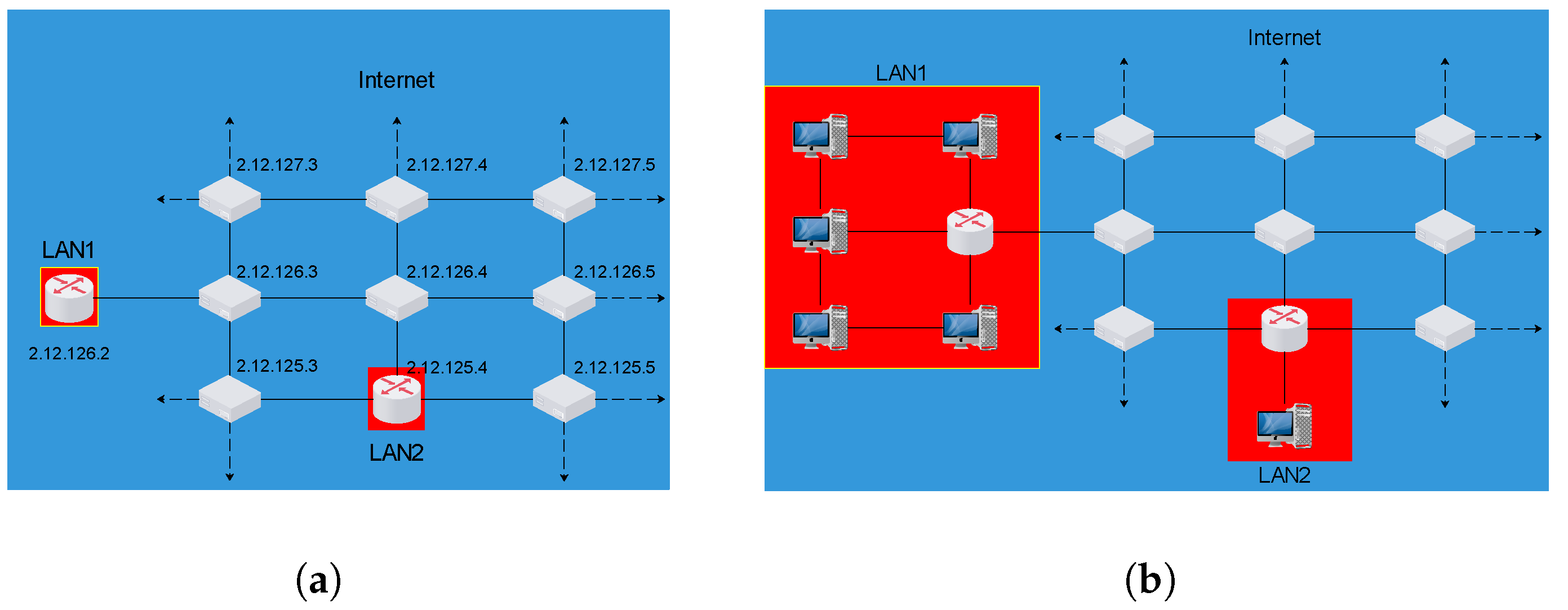
Figure 2.
Image of an internal LAN (I-LAN3 – shown in yellow), placed inside S-LAN3, with its router’s position on the (external) S-LAN3 shifting counter-clockwise. Under appropriate definitions, such a motion can be associated with intrinsic angular momentum, even though the whole LAN3 still seems point-like from the point of view of an outside observer (just like LAN1 of Figure 1(a)).
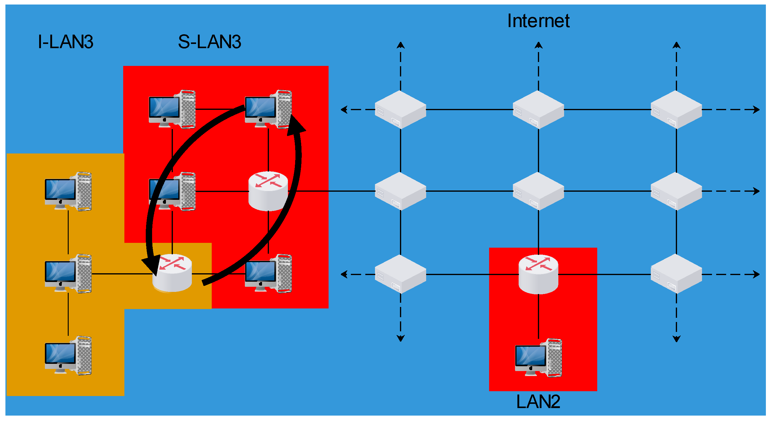
Figure 3.
Figure depicting the path on the network that a signal from node of I-LAN3 should follow in order to arrive to node of LAN2. The yellow arrows are steps on the Internet (i.e., depend on the distance between the two LANs), whereas the green arrows are steps inside a LAN and due to the rotation of I-LAN3 inside S-LAN3 depend on its phase.

Figure 4.
Figure of a 2D slab of átmita with an unoccupied position to the left of átmiton A. This hole results in its four neighbors each having an open port (red lines). Each of them will broadcast a signal with the details of the hole. The corresponding signal sent by átmiton A is []() in its local frame, which will be translated upon arrival at átmiton B to signal []() in the corresponding frame of reference. As the aforementioned signal-translation is trivial, it follows that both A and B belong to the same LAN, (see text).
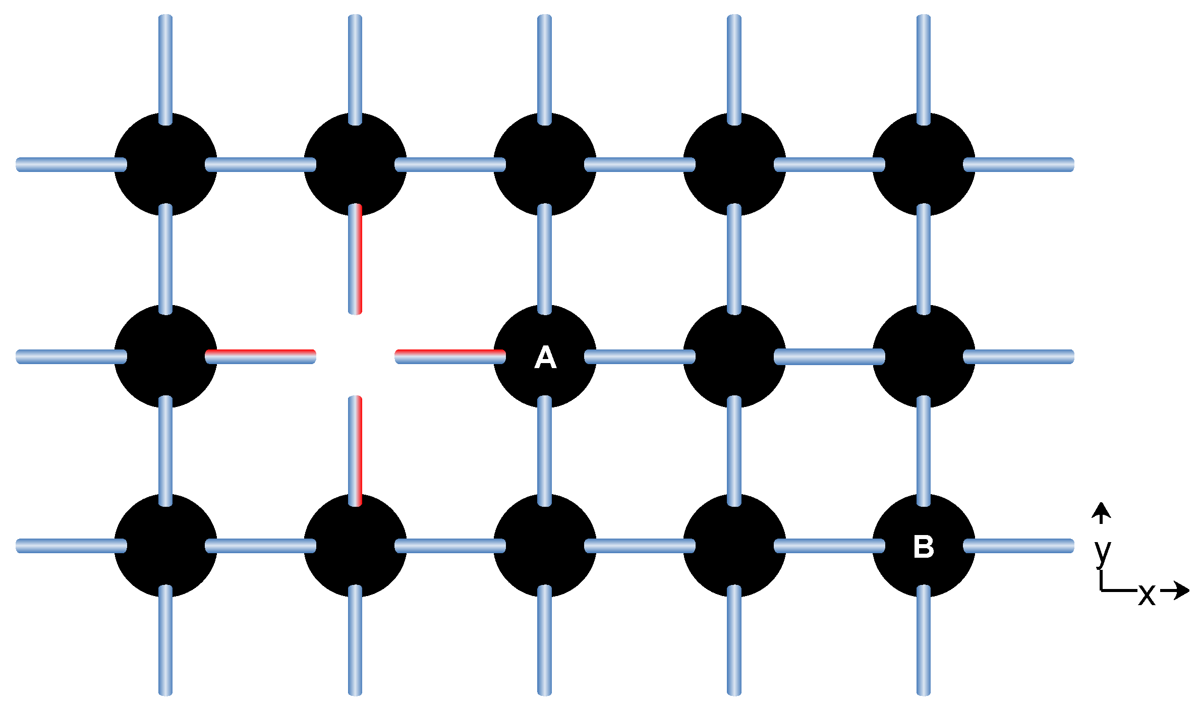
Figure 5.
Map of connections between átmita in a portion of Space (shown in 2D) (a) before and (b) after adding a LAN (consisting of a single átmiton, denoted as G) at the central position of the shown network, with the Space átmiton denoted as R acting as the router connecting the new LAN with Space. Red lines denote open connections and blue existing ones, while the open gray circle emphasizes the fact that router R has now an open port towards its local [-] direction. The connection of the new LAN in the y-axis of router átmiton R is fixed (see Section 3.5), whereas the fact that the broken Space bonds shown in this figure are in the x-axis, indicates that during the next gyros the LAN can move towards either the [-] or [+] directions by its router swapping positions with the corresponding neighboring Space átmiton (green arrows).
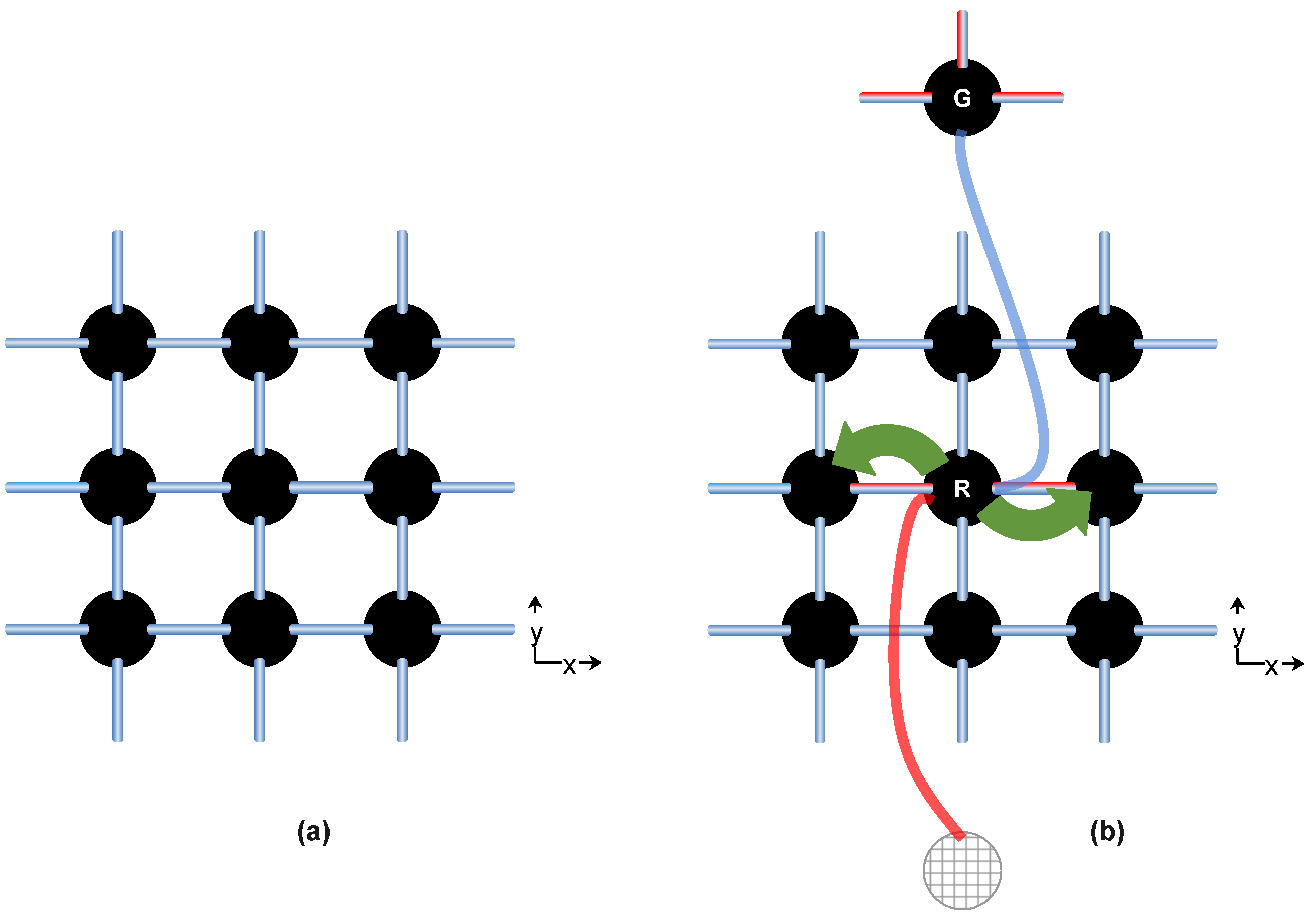
Figure 6.
Two pedestrians walking beside each other with the same speed of 1/, going from point A to point B. One of them (depicted in green) walks on the regular pavement, while the other (red color) walks on a conveyor belt, opposite to its motion. Obviously, the latter one will arrive to the destination later. This is analogous to how space defects produced by macroscopic objects are suggested to create an effective curvature.
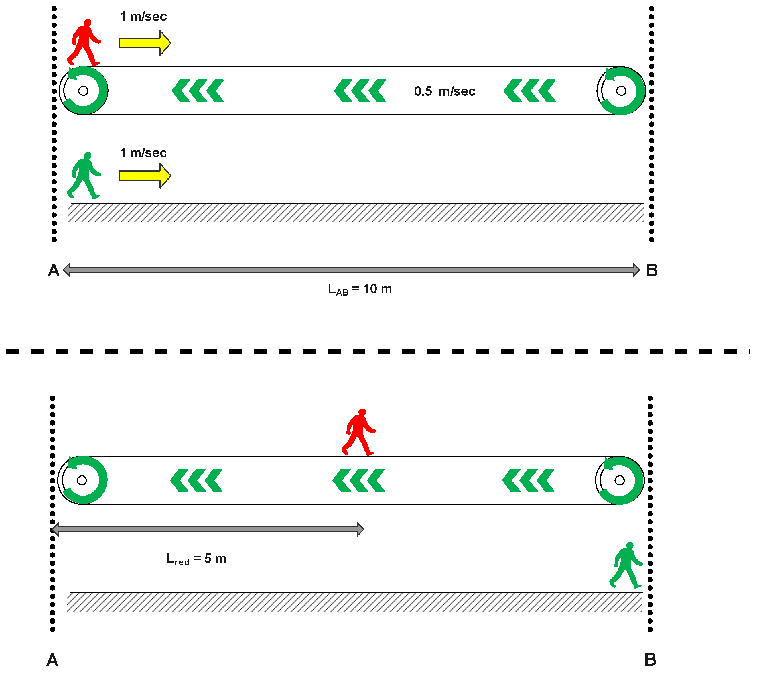
Figure 7.
Inset: Time-evolution of the apparent DE density, as seen by a matter-made observer, normalized to its long-time limit. Main panel: apparent expansion – in semi-log scale – of the normalized length of a given line segment. Here we assume an exponential increase of the number of DE particles inside the given region of “empty” Space, due to their interactions that gradually break high energy particles in more, lower energy ones (see text and Supplementary Section ??). Note that in this example calculation the rate of DE decay was selected in order to provide a reasonable agreement with the current understanding of DE abruptly “turning on” (as seen by matter-made observers) roughly 6 billion years ago (at the the transition redshift [48]). For a discussion on the derivation of the above, see Supplementary Section ??.
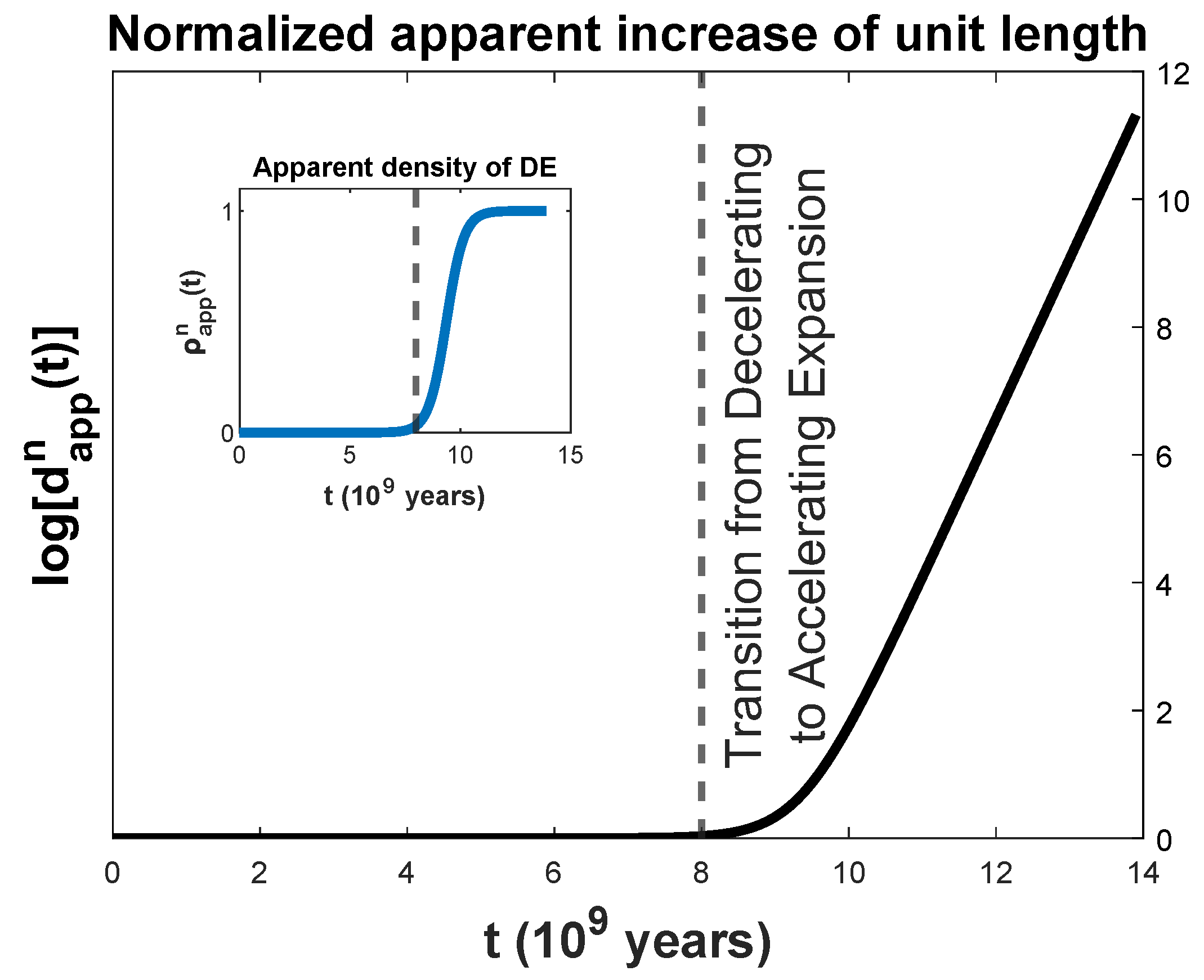
Figure 8.
Image detailing how Protocol 2b leads to every particle’s LANs having a quasi-2D shape. (A) A Z-based particle with a thin and narrow substrate. Near the center of it, there are “excess” new átmita, collectively denoted as N. These are close enough to all open surfaces (shown in thick black) to interact with them. But due to Protocol 2b, they will prioritize the open surfaces on the -plane and move towards them, reach them and turn into substrate themselves, thus widening the substrate (Supplementary Section ??). (B) When the above process continues for long enough, the open surfaces on the -plane will become out-of-bounds (C) the rest of átmita N (that are left after the end of steps A-B) will have to move towards the local z-axis, causing the particle to stand still in Space for the duration of their motion, in accordance to Protocol 2b. (D) At the end of the process, when either all átmita N have been turned into substrate, or the z-thickness of the substrate approaches the maximum value (see Supplementary Section ??), the particle will have a quasi-2D shape, with only the surfaces normal to the local z-axis still in-bounds of the memory of the particle’s router.
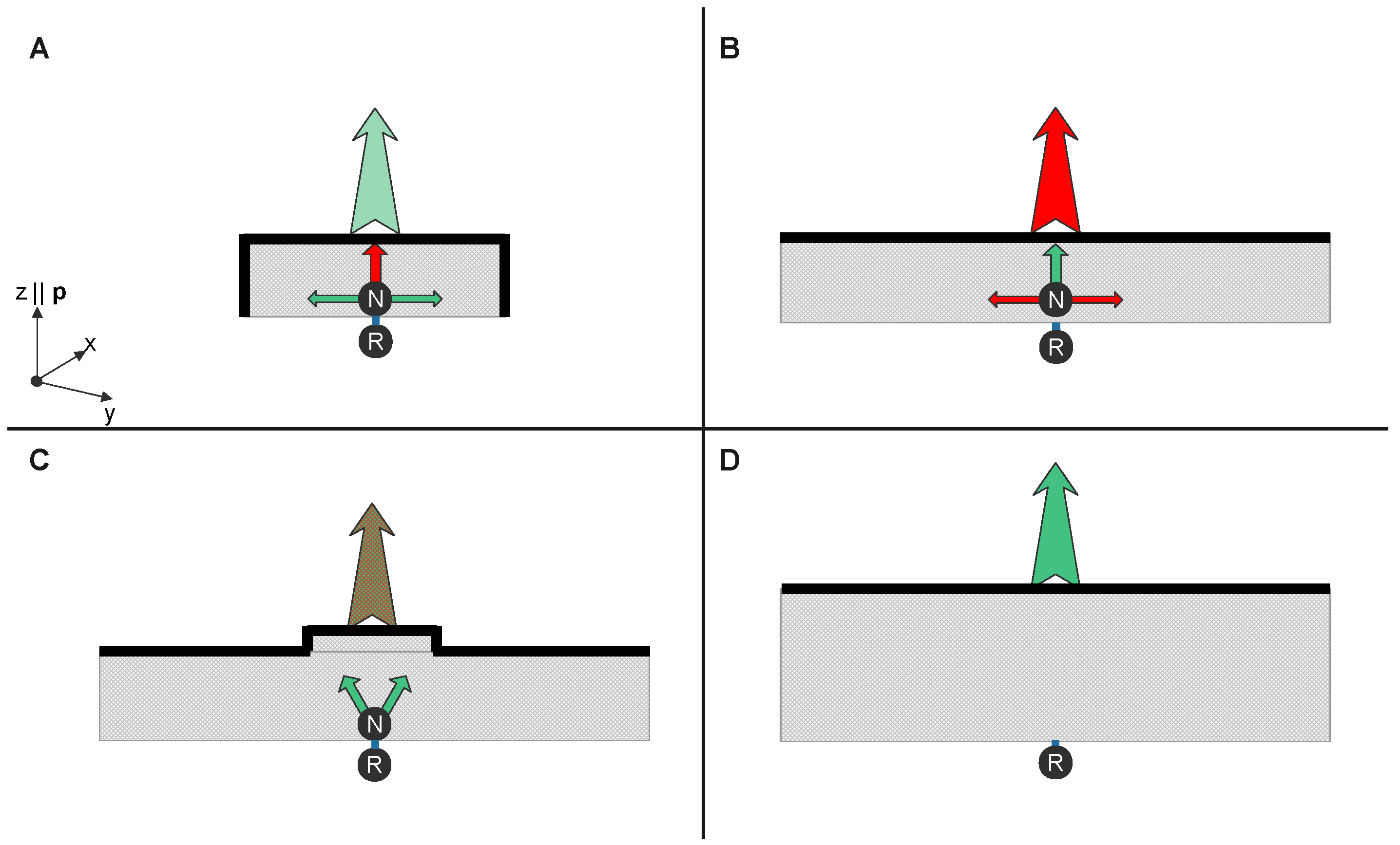
Figure 9.
Outline of the system’s structure : Each gray area corresponds to a LAN of átmita. The router R is connected to the positive and the negative substrates, with an impassable wall separating the two substrates (red dashed line, see Section 5.4). The black dashed lines are the mirror surfaces, from which all the internal addresses are reflected when the particle sends signals through Space. Here only the four surfaces normal to the local z-axis are shown (denoted as SPI(-) and SPE(+) for the positive LAN and SNI(+) and SNE(-) for the negative LAN) since they are the only ones that are relevant (see Section 5.2). For a discussion on the nomenclature of these surfaces, see Supplementary Section ??.
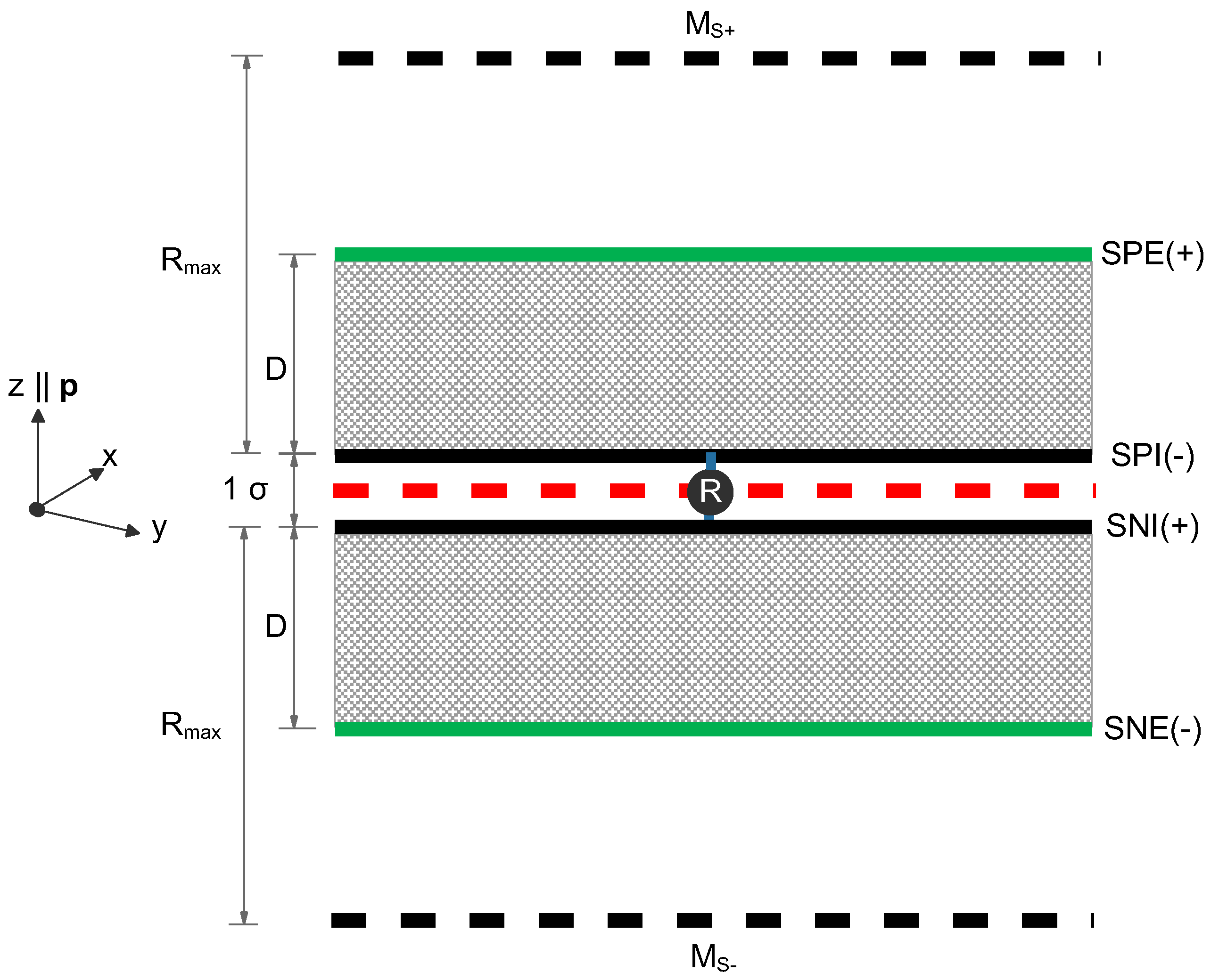
Figure 10.
An electron shown in the coordinate system of its router. For a discussion on the characteristics of this system and a derivation of certain properties of the electron, see text and Supplementary Section ??.
Figure 10.
An electron shown in the coordinate system of its router. For a discussion on the characteristics of this system and a derivation of certain properties of the electron, see text and Supplementary Section ??.
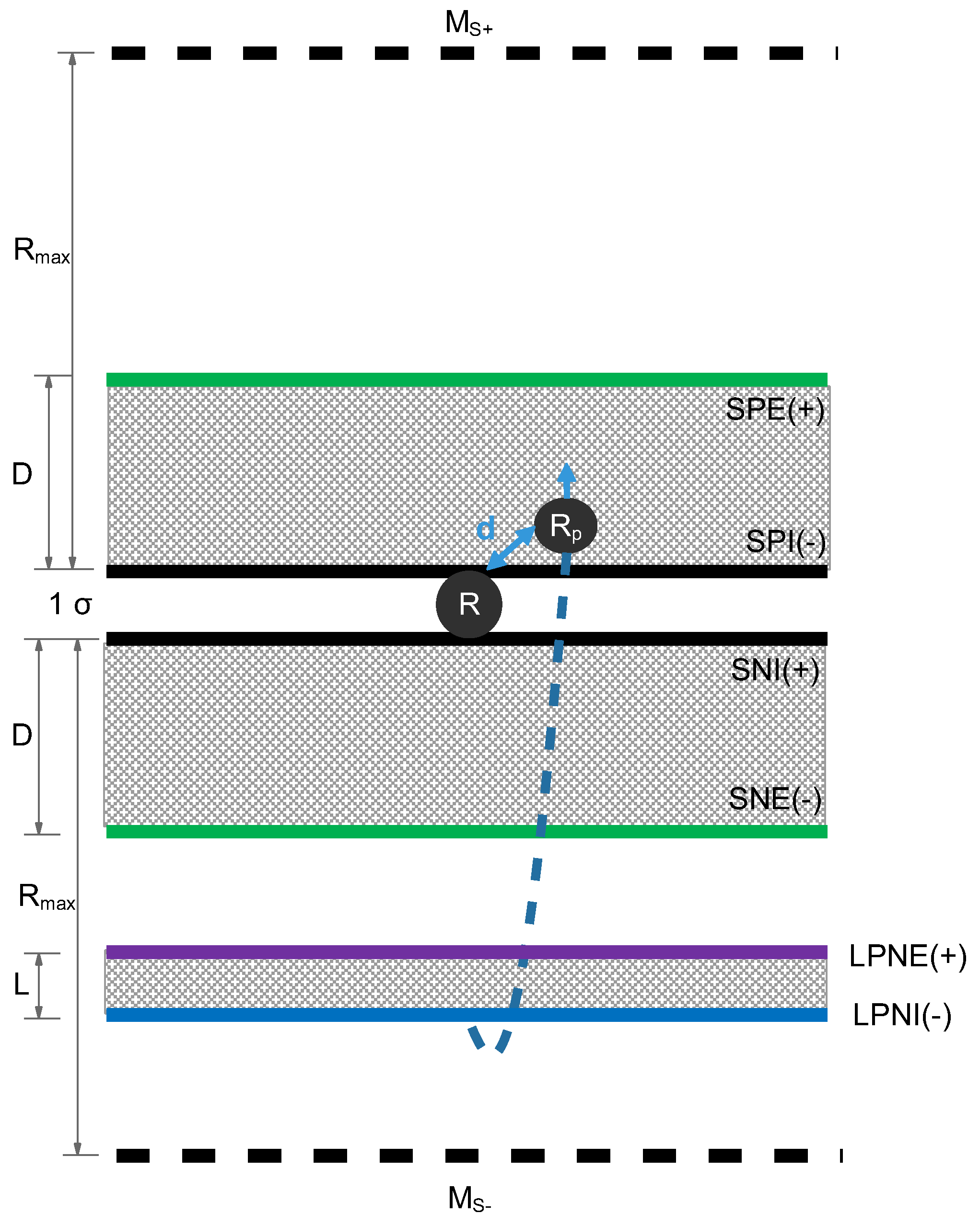
Figure 11.
Figure depicting the configuration of system , which is suggested to correspond to the boson, shown in its router’s coordinate frame. (a): If the internal LANs’ addresses are reflected the way the structure of this system suggests, then there will be address-collisions (shown as a red background color). (b): Due to Protocol 5, this can be avoided if the two internal LANs take turns “tunneling”, i.e., change their basis of reflection from z, to either x or y for up to a full period. This would make them effectively “Dark Matter” constituents. As a result, the bosons should have a charge of 1e, not 2e as their structure suggests, and also they should be able to interact with Dark Matter particles. This might provide an explanation regarding the recent anomalous measurement of their masses (see text).
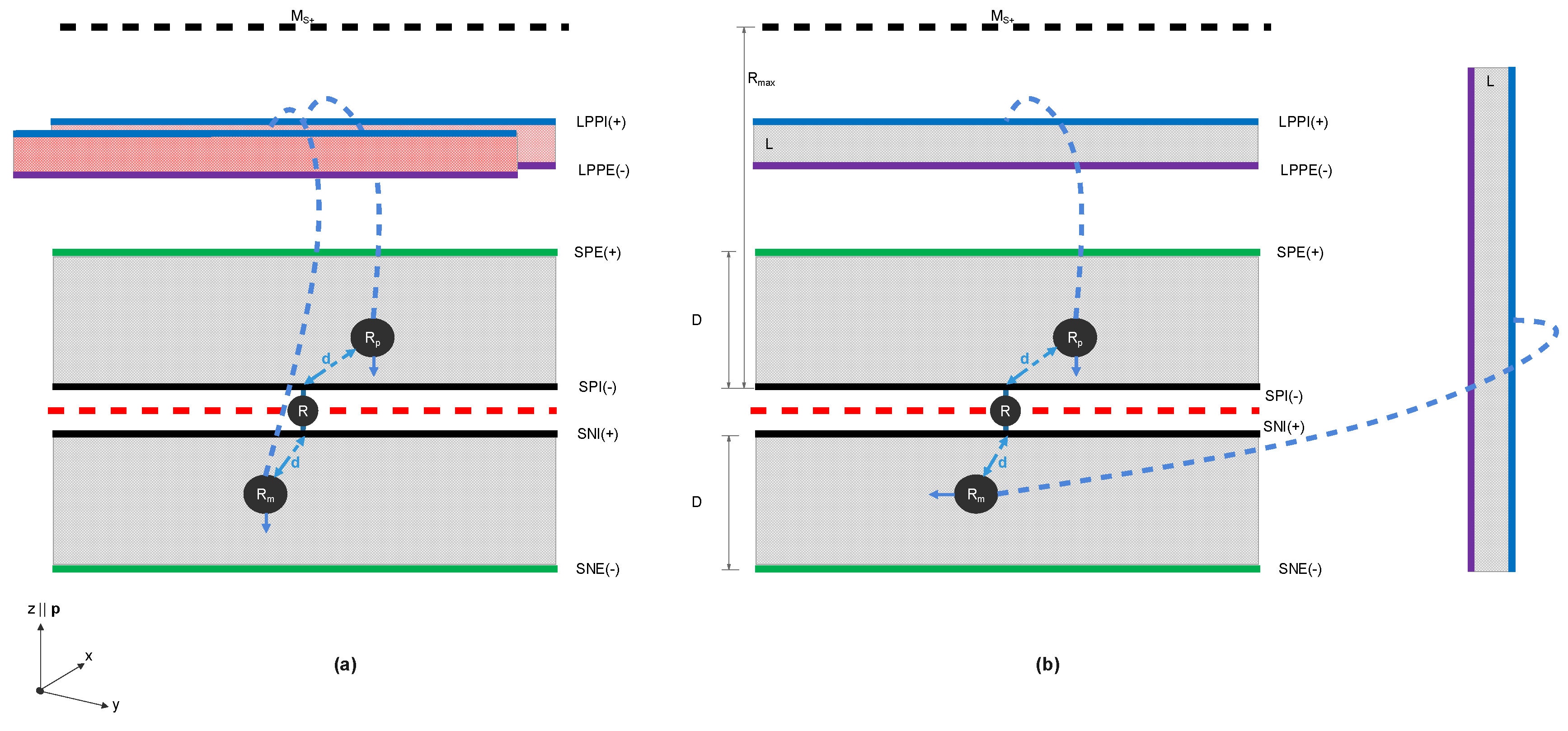

Table 1.
Comparison of the calculated percentages of Regular (baryonic) Matter, , Dark Matter, , and Dark Energy, (from this work) with observations from the primordial universe (WMAP, Plank, BAO), as well as lower-redshift methods (e.g., DES, GalWeight, Pantheon+). The values reported here from Plank (2018) include the Planck CMB temperature, polarization, and lensing power spectra, without including the BAO data. For BAO (2017), the reported value of includes Plank (2015) measurement for the flat CDM model. For DES (2021) it includes galaxy clustering and weak lensing and for DES (2025) BAO, SN, BBN and .
| WMAP (2010) [22] | ||||
| WMAP (2012) [23] | ||||
| Plank (2015) [24] | ||||
| Plank (2018) [20] | 0.0493 ± 0.0014 | 0.264 ± 0.011 | 0.3153 ± 0.0073 | 0.6847 ± 0.0073 |
| BAO (2017) [25] | - | - | - | |
| DES (2019) [26] | - | - | 0.331 ± 0.038 | 0.669 ± 0.038 |
| HSC (2020) [27] | - | - | - | |
| GalWeight (2020) [28] | - | - | 0.310 ± 0.044 | - |
| DES (2021) [29] | - | - | ||
| Pantheon+ (2022) [30] | - | - | 0.334 ±0.018 | - |
| DES (2025) [31] | - | - | 1- = | |
| This work | 0.06 | 0.26 | 0.33 | 0.6 |
Table 2.
The particles of the Standard Model (second column), with their suggested corresponding structures (first column). The index indicates the addition of a LAN, a system and the addition of a system in one of the particle’s substrates. The relevant substrate on which the internal LAN is placed is indicated by the use of a raised or lowered index for the positive and negative substrate, accordingly. The third column details all characteristics (discussed in the text and/or in the Supplementary Information) that help identify each second-order system as that particular Standard Model particle.
| LAN Structure | Standard Model particle | Justification |
|---|---|---|
| G | Boson (Section 5.5), spin-2, stable, massless, interacts only through Gravity (Suppl. Section ??) |
|
| Fermion (Section 5.5), stable, EM q=-1, Weak charge, much less massive than (Suppl. Section ??) |
||
| Antiparticle of (Section 5.4) | ||
| unknown | (highly unstable, , see Section 5.7 and Suppl. Section ??) |
|
| unknown | Antiparticle of (Section 5.4) | |
| Boson (Section 5.5), spin-1, no longitudinal spin component, stable, massless, participates in EM, q=0 (Suppl.Section ??) |
||
| Boson (Section 5.5), unstable (Section 5.7), massive, spin twice that of , participates in EM, q=0 (Suppl. Section ??) |
||
| Boson (Section 5.5), unstable (Section 5.7), massive, Weak charge, participates in EM, q=-1 (Section 5.9) |
||
| Antiparticle of (Section 5.4) | ||
| Fermion (Section 5.5), does not participate in EM (Section 5.9), Weak charge, no color (Section 5.10) |
||
| Antiparticle of (Section 5.4) | ||
| d | Fermion (Section 5.5), massive, negative fractional charge,color via internal tunneling (Section 5.10) |
|
| Antiparticle of (Section 5.4) | ||
| u | Fermion (Section 5.5), massive, positive fractional charge, color via internal tunneling (Section 5.10) |
|
| Antiparticle of (Section 5.4) | ||
| H | Boson (Section 5.5), more massive than , unstable (Section 5.7), does not participate in EM (Section 5.9) |
Disclaimer/Publisher’s Note: The statements, opinions and data contained in all publications are solely those of the individual author(s) and contributor(s) and not of MDPI and/or the editor(s). MDPI and/or the editor(s) disclaim responsibility for any injury to people or property resulting from any ideas, methods, instructions or products referred to in the content. |
© 2025 by the authors. Licensee MDPI, Basel, Switzerland. This article is an open access article distributed under the terms and conditions of the Creative Commons Attribution (CC BY) license (http://creativecommons.org/licenses/by/4.0/).
Copyright: This open access article is published under a Creative Commons CC BY 4.0 license, which permit the free download, distribution, and reuse, provided that the author and preprint are cited in any reuse.


