
Submitted:
15 October 2025
Posted:
16 October 2025
You are already at the latest version
Abstract
Domestic dogs can sense the geomagnetic field (GMF), spontaneously aligning their bodies along its axis, altering alignment's pattern during geomagnetic storms. Whether anthropogenic magnetic fields (MF) from high-voltage power lines (PL) influence this behavior remains unclear. We investigated the effects of alternating MF generated by PL on spontaneous magnetic alignment in 36 dogs. Behavior was recorded under north–south (NS) and east–west (EW) oriented PL and compared with control conditions lacking anthropogenic MF. Each dog’s mean alignment angle relative to magnetic north was calculated from >50 measurements per condition, and Grand Means (GM) were derived. Under control geomagnetically calm conditions, alignment was bimodal (GM = 23°/203°), while geomagnetic storms caused significant shifts and increased angular dispersion. Under NS-oriented PL, alignment remained bimodal (GM = 5°/185°), but under EW-oriented PL it became trimodal (Likelihood ratio test for multimodality: nodes = 3, p = 0.042; GM = 103°/283°). These differences were statistically significant (LME for linearized angles: p < 0.001 for control vs. NS PL and control vs. EW PL). Our results demonstrate that dogs maintain directional alignment under PL exposure, with orientation patterns corresponding to the direction of both MF and PL, which suggests a potentially complex impact involving non-magnetic cues.
Keywords:
alternating magnetic field
; geomagnetic storms
; magnetoreception
; mammal ethology
; spontaneous magnetic alignment
1. Introduction
The effects of the industrially created magnetic fields (MF) on animals and humans remain insufficiently studied [1,2], despite their relevance for technological development on all levels, especially for infrastructure planning and equipment installation. The health impacts of high-voltage power lines (PL), which generate alternating MF below 300 Hz (classified as extremely low frequency) has been investigated primarily in relation to carcinogenic [3,4], teratogenic [5,6,7], cardiovascular, reproductive and developmental outcomes [8,9,10]. Behavioral and physiological changes in animals exposed to alternating MF of varying intensities have been reported [11,12,13], and in some cases explained, albeit controversially, through the ‘parametric resonance model’ which attributes them to interactions between MF and specific ions in living tissues [14,15,16]. By contrast, the influence of alternating MF on spatial orientation in animals – particularly in relation to their natural magnetic sense, or magnetoreception – remains poorly understood and received limited attention [17,18,19,20,21,22].
Magnetoreception is most widely studied in the context of perceiving the geomagnetic field (GMF) which typically exhibits magnetic induction of 50±20 µT. Many vertebrates rely on GMF for navigation during homing and migration [23]. In addition to migratory birds, more than 30 mammal species have been shown to use magnetic clues for long-distance navigation, hunting, and other orientation-related behaviors (see reviews in [24,25]. Recently, magnetoreception has been demonstrated in domestic dogs, which are readily available and suitable test subjects for behavioral experiments [26,27,28,29,30,31].
Several mechanisms have been proposed to explain magnetoreception in animals, with the most frequently addressed being the radical-pair mechanism and magnetite-based receptors. The radical-pair mechanism studied primarily in migratory songbirds, Drosophila and more recently in mammals [32,33,34] relies on photochemical reactions in blue-light–sensitive flavoproteins (cryptochromes) located in the retinal tissue. These reactions lead to the formation of radical pairs in flavin adenine dinucleotide and tryptophan ([FAD•− TrpH•+]), whose interconversion between singlet and triplet states can be influenced by weak magnetic fields, thereby generating directional responses in retinal neurons. This mechanism is light-dependent, provides information on the inclination rather than the polarity of the geomagnetic field (GMF), and therefore cannot distinguish poleward direction. In contrast, magnetoreception based on the alignment of superparamagnetic magnetite crystals Fe3O4 does not require light and can detect the polarity of the horizontal GMF component. The evidence for this mechanism has been reported in bats, Ansell’s mole-rats, and migratory fish [35,36].
One external manifestation of magnetic sensitivity is the spontaneous aligning of the body axis along GMF lines, commonly termed ‘magnetic alignment’ [23]. This phenomenon was first documented in insects and later in fish, caudate amphibians, reptiles, birds, and mammals [26,37,38,39,40,41,42,43]. It was hypothesized that the magnetic alignment aids in reconciling external environmental cues with the animal’s internal cognitive map, thereby reducing its spatial complexity and demands on memory [24,44]. In dogs, excretion serves as form of scent-marking, functioning as a ‘bulletin board’ or even ‘property line’ [45]. Alignment during urination or defecation may thus assist in marking a location within the animal’s cognitive map and in facilitating its later recall.
Natural phenomena from beyond Earth (solar wind and flares) cause frequent fluctuations in the GMF known as geomagnetic storms. In addition, anthropogenic sources, including high-voltage PL, generate alternating MF that superimpose on static GMF, producing magnetic disturbances. Exposure to such oscillating MF has been shown to affect spontaneous magnetic alignment in animals; in dogs, rapid changes in GMF declination during GMF disturbances shifted alignment direction, increasing scattering of bearings to the state of almost disrupted alignment during strong magnetic storms [26]. On the other hand, [46] reported that high-voltage PL disrupted spontaneous alignment of ruminants, with bearings scattering effect attributed not only to oscillations in the MF direction but also to ~12% oscillations in MF intensity – an effect inconsistent with both magnetite-based polarity compass and light-dependent inclination-based magnetoreception.
The physical basis of these phenomena is illustrated in Figure 1 and Figure 2. In the absence of artificial MF sources or strong natural anomalies, animals rely solely on GMF as a magnetic cue. GMF properties (direction, declination, inclination, and magnetic induction indicative for the field strength) are shown in Figure 1. High-voltage PL generate alternating MF at 50 Hz (the standard frequency in the Czech Republic). These fields reach their maximum intensities directly beneath PL, at mid-span between pylons where conductor sag brings the lines closest to the ground: approximately 15 µT for 380 kV, 8 µT for 220 kV, and 5 µT for 110 kV lines [47,48]. At such locations, the relevant orientation cue is not the GMF itself but the resultant total field T, defined as the vector sum of GMF (B) and the wire-generated MF (W) according to the superposition principle. T oscillates 50 times per second within a defined angular range determined by the relative orientation of PL relative to GMF (Figure 2). It seems not impossible that dogs can perceive alternating magnetic cues of this oscillating field, as the 50 Hz frequency falls within the neural processing range for both their visual and somatosensory stimuli [49]. However, the presence of multiple, rapidly changing magnetic signals deviating from magnetic north may interfere with their magnetic sense, potentially causing alignment disruption through compromising either magnetically modulated visual patterns or magnetic compass itself [18].
This study was designed to test the hypothesis that alternating MF generated by high-voltage PL disrupt spontaneous magnetic alignment in domestic dogs, as previously observed in cattle and deer [46]. To evaluate this, we recorded and analyzed the spontaneous body alignment of dogs during excretion (urination and defecation) under conditions with and without detectable ELF MF generated by overhead PL.
2. Materials and Methods
2.1. Data collection
The study was conducted at 38 locations across the Czech Republic between 15 April 2013 and 25 June 2015. We recorded the body alignment of 36 healthy dogs freely moving off the leash – 22 males and 14 females belonging to 18 breeds and three crossbreeds, aged from 1 to 13 years (Supplementary material, Tables S1, S2). Magnetic alignment was quantified as the angular position of the thoracic spine axis relative to magnetic north (Figure 3). Observations were made during dog’s spontaneous urination and/or defecation, following the procedure described in [26]. Owners, trained in the protocol, recorded hand compass bearings (precision ±5°) while walking their dogs in designated areas. For each dog, 54-776 control measurements and 48-378 experimental measurements were collected throughout the day across the study period, yielding a total of 24,217 measurements. Data from [26] were excluded; all analyses are based solely on newly collected data.
In control conditions, dogs were roaming freely in open rural habitats (meadows, fields) located at least 500 m from potential confounding features such as linear structures or anthropogenic magnetic noise sources that could potentially affect dogs’ magnetic sense (such as fences, walls, motorways, powerlines, large metal constructions). Experimental observations were conducted at comparable rural locations situated directly beneath high-voltage PL. Bearings were taken when dogs were positioned under the PL wires at least 10 m away from pylons. Selected PL were oriented either north-south (NS) or east-west (EW) with respect to true (not magnetic) north, as determined using Google Maps. Creating sham PL (lines without current) was technically unfeasible for obtaining a statistically robust dataset.
For each measurement, the time (±1-10 min) and date of collection were recorded. Continuous magnetograms corresponding to all the observation dates were obtained from the Geomagnetic Observatory Fürstenfeldbruck in Munich, Germany (http://www.geophysik.uni-muenchen.de/observatory/geomagnetism) and used to calculate relative changes in GMF declination [26]. Time-specific GMF parameters (Bx, By, Bz) for the experimental locations and dates were retrieved from the NOAA database (https://www.ngdc.noaa.gov).
2.2. Statistical analyses
We conducted the procedures of first- and second-order circular statistics and generated graphs in Oriana v4.02 (Kovach Computing Services, 1994-2013). Additional statistical analyses were performed in R Studio v. 2023.03.0 (Posit Software, PBC, 2009-2023, packages circular, CircStats, NPCirc for the circular statistics, and lme4 for mixed models of linearized angular data). MF vector calculations and visualizations were conducted in Mathematica 13.0 (Wolfram Research).
Previous work [26] demonstrated that the percentage of relative change in GMF declination (RCD) provides a more informative marker of geomagnetic conditions than the Kp index for in studies of spontaneous magnetic alignment. In this study, RCD was calculated as the difference between minimum and maximum of GMF declination during a defined disturbance period, expressed as a percentage of 360 arch minutes divided by the disturbance duration, as measured on magnetograms. RCD values were determined for each time point of data collection and were used to categorize angular measurements into ‘magnetic calm’ (RCD = 0%) or ‘magnetic disturbance’ (moderate, RCD ≤ 2%, strong, RCD > 2-3%).
Compass-based azimuth measurements differ from true north by a location-specific angle of declination (D). Consequently, the direction of PL wires in our observations did not perfectly align with, nor remain strictly perpendicular to, the GMF induction vector (B). Parameters of the total MF beneath PL were calculated using averaged values of Bx, By, Bz across the study period and across location groups (PL oriented geographically, rather than magnetically, NS or EW).
Given a compass measurement error of ±5°, raw angular data were binned into 10° classes. As an initial inspection, both the complete dataset and individual sub-datasets (each for one dog with > 10 measurements) were examined for evidence of bi- or multimodality, we applied visual observation and likelihood ratio test for circular multimodality [50]. We calculated basic circular statistics (mean vector µ, mean vector length r, circular standard deviation CSD, and concentration parameter k), as well as second order statistics (Grand Mean vectors, Moore’s Modified Rayleigh Test for non-uniformity of axial grouped data). One-sample test (Rayleigh’s Uniformity Test) was applied to assess departures from uniform distribution. As measures of scatter, we employed r as an indicator of concentration and k as a measure of dispersion [51,52].
Standard tests for comparing two circular means – Hoteling’s Two Sample Test and Moore's Paired Test [53] – are not applicable to grouped circular data. To address this, we used a MANOVA-based approach recently proposed by [56]. This method linearizes circular values by converting each angle into sine and cosine components, which can then be analyzed using conventional MANOVA (R packages stats, MANOVA.RM) or linear models that accept paired data. For group comparisons, we applied linear mixed-effects model (LME) to linearized circular data, designating individual dogs as a random factor, and including dog-specific characteristics (sex, age, weight, breed, owner) as fixed factors.
2.3. Ethical statement
This work did not require ethical approval from a human subject or animal welfare committee.
3. Results
3.1. Differences in alignment during geomagnetic calm and during the periods of geomagnetic disturbances
The distribution of bearings in both control conditions and beneath PL wires was axial as suggested by visual inspection and multimodality test (Figure 4). The Grand Means (GM) calculated from the individual axial means (each mean is calculated from > 50 bearings of one dog) at any RCD were 35°/215° in control (36 dogs), 2°/182° under NS-directed PL (36 dogs), and 108°/288° under EW-directed PL (34 dogs). Overall, bearings were widely scattered around 360° (Figure 4a). However, during the periods of magnetic calm (RCD = 0%) bearings became more concentrated along the NS or EW axis (Figure 4b): GM was 23°/203° in control, shifting to 5°/185° under NS-oriented PL, and to 103°/283° under EW-oriented PL. Interestingly, the distribution of mean angles under EW-directed PL was trimodal (Likelihood ratio test for multimodality: estimated number of nodes=3, p=0.042)
Previous work [26] demonstrated that dogs’ alignment deviates progressively from the NS axis (relative to magnetic N) with increasing geomagnetic disturbance, shifting entirely toward the EW axis when RCD exceeded 2%. Our data showed the same trend (Table 1, Figure 5). In control conditions, GM also shifted clockwise during geomagnetic disturbances (Figure 5c, d), and this effect was highly significant (LME: F = 6.12, p = 0.0022). In contrast, under NS-oriented PL wires, alignment changed only slightly (Table 1), with differences that were not significant (F = 0.23, p = 0.79). Under EW-oriented PL, alignment showed a minor clockwise shift, but again changes were not significant (F = 0.59, p = 0.55).
To evaluate the effect of geomagnetic disturbances on concentration of bearings, we used standard circular measures: mean vector length (r) and concentration parameter (k). In control conditions, both r and k decreased with increasing geomagnetic disturbance (Table 1) indicating greater dispersion of bearings during disturbed periods. These reductions were statistically significant (LME: Fr = 4.749, p = 0.012; Fk: = 5.348, p = 0.007). Under NS-oriented PL, r and k showed only minor, non-significant changes (LME: Fr = 0.852, p = 0.43; Fk: = 1.885, p = 0.16). Under EW-directed PL, r and k decreased more markedly (k = 0.322), but these changes were likewise non-significant (LME: Fr = 0.573, p = 0.57; Fk: = 0.573, p = 0.99).
3.2. Predictions for the total magnetic field direction under the power lines
As described above, beneath PL wires the horizontal component of the total field (TB) is the vector sum of the GMF horizontal component (Bh) and the field generated by the wire (W, ~20 µT in the studied power lines) that is lacking vertical component. Th alternates symmetrically around its median at a frequency ~50 Hz. Across all observation sites, the total GMF ranged from 44.1792 to 49.1076 µT, with field parameters summarized in Table 2 (see Supplementary material, Table S1.2 for location details). Mean values of magnetic induction, declination (D, α0), and inclination (I, β0) were calculated for each condition (Table 2).
In control locations (no PL):
Bctr = (Bx, By, Bz) = (19.9830, -1.2373, 44.5499), |Bctr| = 48.8982 µT, Dctr = 3.55°, Ictr = 65.81°.
For locations with NS-oriented PL (outside the impact of PL):
BNS = (Bx, By, Bz) = (19.9596, -1.2149, 44.6225), |BNS| = 48.8157 µT, DNS = 3.48°, INS = 65.86°.
For locations with EW-oriented PL (outside the impact of PL):
BEW = (Bx, By, Bz) = (19.9784, -1.1925, 44.6184), |BEW| = 48.9015 µT, DEW = 3.41°, IEW = 65.84°.
We then calculated magnetic induction of the total field T = B + W separately for NS- and EW-oriented PL (Table 2, Figure 5). Directly beneath NS-oriented PL, the horizontal component of T alternated between Th1 = 27.4092 µT and Th2 = 29.1283 µT, with the amplitude angle Δα = 45.0° (Figure 5a, the vector lengths and the angles are scaled). The median azimuth between α1 and α2 was 356.5°. Inclination angles (not shown in Figure 5 but listed in Table 2) deviated from INS by -7.46° and -23.06°, yielding Δβ = 15.6°. The resulting inclination of T was shallower than that of GMF (I), implying that under an inclination-compass scenario a dog would experience -20° directional shift compared with control conditions.
Directly beneath EW-oriented PL, the horizontal component of T alternated between Th1 = 39.9961 µT and Th2 =1.1907 µT, Δα = 89.33° (Figure 5b). The mean angle between α1 and α2 was 43.8°. Left extreme of T was oriented approximately north and the right extreme toward east. Inclination angles β1 and β2 deviated from IEW by -17.7° and 22.7°, respectively, with Δβ = 40.4°.
3.3. Impact of power lines on dogs’ alignment
To test the hypothesis that alignment would be disrupted (and the bearings scattered) beneath PL, we used r and k as the measures of concentration/dispersion of bearings, and compared these two parameters calculated from control data with those characterizing the alignment under the PL.
As shown in the previous section, total r and k values calculated from bearings recorded under PL were higher than those in control. This indicates that dogs’ alignment did not disappear under PL; to the contrary, the bearings were less scattered: total rcontrol = 0.064, rNS = 0.125, rEW = 0.124; total kcontrol = 0.127, kNS = 0.251, kEW = 0.251. These differences were statistically significant (LME: Fr = 22.328, p = 0.0017; Fk = 19.471, p = 0.0024).
Nevertheless, marked changes in alignment pattern and direction were observed beneath high-voltage PL. In control conditions, dogs oriented primarily along 23°/203° (relative to magnetic north) during geomagnetic calm, with bearings concentrated along the NS axis relative to magnetic N (Figure 5a, b; Supplementary material, Table S1.5). Under geographically NS-oriented PL the bearings remained concentrated along the magnetic NS axis (GM = 5°/185° relative to magnetic N, RCD=0%). In contrast, under geographically EW-oriented PL, dogs aligned either along the NS axis or perpendicular to it (trimodal distribution, GM = 103°/283° relative to magnetic N, RCD=0%). This difference in alignment was highly significant (LME for linearized angles: F = 48.758, p <0.001 for control vs. NS PL, F = 90, p <0.001 for control vs. EW PL).
4. Discussion
Research on magnetoreception in large mammals remain challenging, as controlled laboratory experiments involving animal immobilization or direct brain electrophysiological recordings are ethically and technically unfeasible. Experiments with dogs in large magnetic coils have produced promising results [30], although these methods require further refinement. As an alternative, broad-scale observations of animals in natural settings provide a viable approach, particularly when individuals display spontaneous behaviors previously demonstrated to reflect magnetic orientation [26,39,40,46]. In this study, we analyzed a large dataset (> 24,000 measurements) collected under conditions where magnetically mediated behavior was expected to be either unaffected (control) or influenced by potentially disruptive factors, specifically the alternating MF generated by high-voltage PL.
Comparison of dogs’ body alignment across control conditions and under PL oriented along NS or EW axes showed that high-voltage PL induced directional changes but did not disrupt alignment, in contrast to the disruption reported in cattle and deer [46]. Some scattering of bearings was observed when dogs were exposed to PL during geomagnetic disturbances; however, this scattering was much less pronounced than in control conditions. The most straightforward explanation of this phenomenon would be that, in the absence of static, non-oscillating magnetic cue of the GMF intensity, dogs may switch completely from magnetoreception to relying on prominent visual cues for orientation, and align accordingly (for example, in the direction of PL pylons). However, this explanation does not account for the increase, although only slightly, in scattering of bearings observed during geomagnetic disturbances under PL in comparison with the periods of geomagnetic calm (Figure 4c,d). Nor does it adequately explain the trimodal alignment pattern observed under EW-oriented PL that contains NS and EW component (Figure 4, EW wires) which is different from orienting observed under EW-directed PL in the domestic cattle.
The geomagnetic environment at the time of recording can significantly influence animal behavior and physiology [55,56], including directional alignment in dogs [26]. Under geomagnetic calm and in the absence of non-geomagnetic MF sources, dogs exhibit spontaneous alignment along the NS axis. During magnetic disturbance, such alignment significantly departs from the NS axis, introducing additional information noise that can be source of false positives and false negatives. Since there is variation in direction and strength of GMF, including small reversible variations due to solar activity, only the days and time of magnetic calm should be selected to evaluate the significance of other factors in directional alignment.
The sensitivity of dogs to even minor GMF disturbances suggests an ability to detect weak MF and their subtle directional changes. Prior to this study, it remained unclear whether dogs can perceive alternating MF or discriminate between two oscillating MF vectors. Our results confirm the conclusions of [26] that in the absence of PL and during geomagnetic calm, dogs aligned along the NS axis (Figure 4b, control/no wires), but this alignment disappeared during geomagnetic disturbances (Figure 4c,d control/no wires). Under NS-oriented PL, dogs predominantly aligned in NS direction during magnetic calm periods (Figure 4, NS wires), consistent with the total field median direction (median of the two alternating MF vectors beneath the wire) and PL orientation. In contrast, under EW-oriented PL two perpendicular alignments were observed during geomagnetic calm conditions (Figure 4, EW wires) roughly correspond to the two alternating MF vectors beneath the wire, and PL orientation. The intensity of total field T (Figure 5, Table 2)
The observed patterns seem to be more complex than a simple shift from magnetoreception to reliance on visual cues. (e.g. pylons as the overhead wires are not clearly visible for roaming dogs and do not constitute a simple directional cue). Another, although less parsimonious explanation may be that dogs combine both visual and magnetic (even if oscillating) cues for orientation. As highlighted in the review on the ‘noisy’ nature of animal magnetoreception [57], non-magnetic cues may complement the magnetic sense, which alone provides neither rapid nor continuous directional information. Experimental evidence from Bogong moths [58] supports such a multimodal orientation system, in which magnetic input is integrated with visual cues. Similarly, avian navigation is as well established as multimodal, relying on sun, stars, and magnetic compass [23].
The temporal resolution of the cone cells in the canine retina is higher than in humans, reaching 70-80 Hz, while the critical flicker fusion of rod cells is similar in both species (~20Hz) [49]. This suggests that dogs may be able to detect, albeit during daylight, visual flickering at frequencies above 50 Hz. However, it would be speculative to assume that they can also perceive MF oscillating at this frequency as a discrete cue, or use it for orientation, and further research is needed on this matter.
The intensity of the total field T (Figure 5, Table 2) in this study was 1.4 times higher than that of B, exceeding by far the sensitivity range of the inclination compass estimated for birds [59]. Unfortunately, because we did not record the dogs’ alignment separately on the left and right sides of the wires, as described for cattle in [46], this study does not allow us to determine whether dogs employ a radical-pair–based inclination compass, neither if the observed increase in field intensity (B + 76%) could render the dogs’ magnetic compass non-functional, thereby narrowing the potential causes of the persisting alignment to visual or other cues (e.g., position of the Sun). Further research is needed to clarify the underlying reasons for the persistence of dogs' alignment under PL.
5. Conclusions
1. Our study provides further evidence of magnetoreceptive abilities in domestic dogs, expressed, among other behaviors, as spontaneous directional alignment. This alignment occurs consistently in the absence of magnetic sources other than the geomagnetic field (GMF) and demonstrates dogs’ sensitivity to minor variations in GMF declination.
2. Under the PL wires, dogs were exposed to an oscillating magnetic stimulus 1.4 times more intensive than the GMF, alternating at 50 Hz, in a direction differing from the GMF vector (41.5° and 311.5° relative to magnetic north under NS-directed PL, and 91.0° and 358.3° under EW-directed PL).
3. Dogs maintain directional alignment under PL, unlike cattle and deer [47]. While the simplest explanation of this phenomenon would be a shift from magnetic to visual cues (like PL pylons) for orientation, the trimodal pattern observed under EW-directed PL (with both NS and EW components) suggests a more complex mechanism, not excluding a combination of magnetic and non-magnetic cues.
Supplementary Materials
The following supporting information can be downloaded at: http://datadryad.org/stash/share/e2T2311ESuJoahA8mdyrwBoWoE8257ty5NIQMNOvFs0 , Table S1: Information about the dogs used in the experiments, locations, and basic statistics; Table S1: Raw measurements of dogs' alignment in control and under PL.
Author Contributions
Conceptualization, VH, HB, KB, JA and NI; methodology, VH, HB, KB, JA and PN; software, NI; validation, VH, HB, NI, KB, JA, and HB; formal analysis, NI; investigation, VH, KB, JA, PN, VH, KT, and JM; resources, VH, TK, MJ and HB; data curation, VH, KB, JA and PN; writing—original draft preparation, NI; writing—review and editing, HB, KB, JA, VH, HB; visualization, HB; supervision, VH, HB; project administration, VH, HB, KB; funding acquisition, VH, HB, MJ. All authors have read and agreed to the published version of the manuscript.
Funding
This research was funded by grant "Advanced research supporting the forestry and wood-processing sector´s adaptation to global change and the 4th industrial revolution", No. CZ.02.1.01/0.0/0.0/16_019/0000803 financed by OP RDE".
Data Availability Statement
The original data analyzed in this paper are publicly available on Dryad repository and can be downloaded at: http://datadryad.org/stash/share/e2T2311ESuJoahA8mdyrwBoWoE8257ty5NIQMNOvFs0.
Acknowledgments
Authors gratefully acknowledge the staff and students of Department of Game Management and Wildlife Biology, Faculty of Forestry and Wood Sciences, Czech University of Life Sciences Prague who helped collecting the data and participating in field experiments. Dr Vitalii Zablotsky is gratefully acknowledged for suggestions on magnetic field theory and help in calculations. Anonymous reviewer of this paper is gratefully acknowledged for critical remarks and suggestions that helped to significantly improve this manuscript.
Conflicts of Interest
The authors declare no conflicts of interest. The funders had no role in the design of the study; in the collection, analyses, or interpretation of data; in the writing of the manuscript; or in the decision to publish the results.
Abbreviations
The following abbreviations are used in this manuscript:
| GMF | Magnetic field of Earth/geomagnetic field |
| MF | Magnetic field |
| PL | Power lines |
| NS | North-south (direction) |
| EW | East-west (direction) |
References
- Saunders, R. Static magnetic fields: animal studies. Prog. Biophys. Mol. Biol. 2005, 87 (2–3), 225–239. [CrossRef]
- Yamazaki, K.; Taki, M.; Ohkubo, C. Safety assessment of human exposure to intermediate frequency electromagnetic fields. Electr. Eng. Jpn. 2016, 197 (4), 3–11. [CrossRef]
- Kheifets, L.; Ahlbom, A.; Crespi, C. M.; Feychting, M.; Johansen, C.; Monroe, J.; Murphy, M. F. G.; Oksuzyan, S.; Preston-Martin, S.; Roman, E.; Saito, T.; Savitz, D.; Schuz, J.; Simpson, J.; Swanson, J.; Tynes, T.; Verkasalo, P.; Mezei, G. A pooled analysis of extremely low-frequency magnetic fields and childhood brain tumors. Am. J. Epidemiol. 2010, 172 (7), 752–761. [CrossRef]
- Repacholi, M. Concern that “EMF” magnetic fields from power lines cause cancer. Sci. Total Environ. 2012, 426, 454–458. [CrossRef]
- Huuskonen, H.; Juutilainen, J.; Komulainen, H. Development of preimplantation mouse embryos after exposure to a 50 Hz magnetic field in vitro. Toxicol. Lett. 2001, 122 (2), 149–155. [CrossRef]
- Brent, R. L.; Gordon, W. E.; Bennett, W. R.; Beckman, D. A. Reproductive and teratologic effects of electromagnetic fields. Reprod. Toxicol. 1993, 7 (6), 535–580. [CrossRef]
- Malagoli, C.; Crespi, C. M.; Rodolfi, R.; Signorelli, C.; Poli, M.; Zanichelli, P.; Fabbi, S.; Teggi, S.; Garavelli, L.; Astolfi, G.; Calzolari, E.; Lucenti, C.; Vinceti, M. Maternal exposure to magnetic fields from high-voltage power lines and the risk of birth defects. Bioelectromagnetics 2012, 33 (5), 405–409. [CrossRef]
- Ahlbom, A.; Feychting, M.; Gustavsson, A.; Hallqvist, J.; Johansen, C.; Kheifets, L.; Olsen, J. H. Occupational magnetic field exposure and myocardial infarction incidence: Epidemiology 2004, 15 (4), 403–408. [CrossRef]
- International Commission on Non-Ionizing Radiation Protection. ICNIRP guidelines for limiting exposure to time-varying electric and magnetic fields (1 Hz – 100 kHZ). Health Phys. 2010, 99 (6), 818–836.
- BioInitiative Working Group. BioInitiative Report 2012: A rationale for biologically-based exposure standards for low-intensity electromagnetic radiation; 2012; pp 1–1479. https://bioinitiative.org/table-of-contents/ .
- Marino, A. A.; Becker, R. O. Biological effects of extremely low frequency electric and magnetic fields: A Review. Physiol. Chem. Phys. 1977, 9 (2), 131–147.
- Kirschvink, J. L.; Padmanabha, S.; Boyce, C. K.; Oglesby, J. Measurement of the threshold sensitivity of honeybees to weak, extremely low-frequency magnetic fields. J. Exp. Biol. 1997, 200 (9), 1363–1368. [CrossRef]
- Prato, F. S.; Desjardins-Holmes, D.; Keenliside, L. D.; DeMoor, J. M.; Robertson, J. A.; Thomas, A. W. Magnetoreception in laboratory mice: sensitivity to extremely low-frequency fields exceeds 33 nT at 30 Hz. J. R. Soc. Interface 2013, 10 (81), 20121046. [CrossRef]
- Zhadin, M. N.; Deryugina, O. N.; Pisachenko, T. M. Influence of combined DC and AC magnetic fields on rat behavior. Bioelectromagnetics 1999, 20 (6), 378–386. [CrossRef]
- Belova, N. A.; Acosta-Avalos, D. The effect of extremely low frequency alternating magnetic field on the behavior of animals in the presence of the geomagnetic field. J. Biophys. 2015, 2015, 1–8. [CrossRef]
- Ermakov, A.; Afanasyeva, V.; Ermakova, O.; Blagodatski, A.; Popov, A. Effect of weak alternating magnetic fields on planarian regeneration. Biochem. Biophys. Res. Commun. 2022, 592, 7–12. [CrossRef]
- Nishimura, T.; Okano, H.; Tada, H.; Nishimura, E.; Sugimoto, K.; Mohri, K.; Fukushima, M. Lizards respond to an extremely low-frequency electromagnetic field. J. Exp. Biol. 2010, 213 (12), 1985–1990. [CrossRef]
- Vanderstraeten, J.; Gillis, P. Theoretical evaluation of magnetoreception of power-frequency fields. Bioelectromagnetics 2010, 31 (5), 371–379. [CrossRef]
- Vanderstraeten, J.; Burda, H. Does magnetoreception mediate biological effects of power-frequency magnetic fields? Sci. Total Environ. 2012, 417–418, 299–304. [CrossRef]
- Kolbabová, T.; Pascal Malkemper, E.; Bartoš, L.; Vanderstraeten, J.; Turčáni, M.; Burda, H. Effect of exposure to extremely low frequency magnetic fields on melatonin levels in calves is seasonally dependent. Sci. Rep. 2015, 5 (1), 14206. [CrossRef]
- Vanderstraeten, Jacques. Champs Magnétiques et Santé : De l’épidémiologie à La Chimie Des Cryptochromes [Magnetic Fields and Health: From Epidemiology to Cryptochrome Chemistry]. Rev Med Brux 2017, 38 (2), 79–89.
- Xie, C. Searching for unity in diversity of animal magnetoreception: From biology to quantum mechanics and back. The Innovation 2022, 3 (3), 100229. [CrossRef]
- Wiltschko, R.; Wiltschko, W. Magnetic orientation in animals; Bradshaw, S. D., Burggren, W., Heller, H. C., Ishii, S., Langer, H., Neuweiler, G., Randall, D. J., Series Eds.; Zoophysiology; Springer Berlin Heidelberg: Berlin, Heidelberg, 1995; Vol. 33. [CrossRef]
- Moritz, R. E.; Burda, H.; Begall, S.; Němec, P. Magnetic compass: a useful tool underground. In Subterranean Rodents; Begall, S., Burda, H., Schleich, C. E., Eds.; Springer Berlin Heidelberg: Berlin, Heidelberg, 2007; pp 161–174. [CrossRef]
- Burda, H.; Begall, S.; Hart, V.; Malkemper, E. P.; Painter, M. S.; Phillips, J. B. Magnetoreception in mammals. In The Senses: A Comprehensive Reference; Elsevier, 2020; pp 421–444. [CrossRef]
- Hart, V.; Nováková, P.; Malkemper, E.; Begall, S.; Hanzal, V.; Ježek, M.; Kušta, T.; Němcová, V.; Adámková, J.; Benediktová, K.; Červený, J.; Burda, H. Dogs are sensitive to small variations of the Earth’s magnetic field. Front. Zool. 2013, 10 (1), 80. [CrossRef]
- Martini, S.; Begall, S.; Findeklee, T.; Schmitt, M.; Malkemper, E. P.; Burda, H. Dogs can be trained to find a bar magnet. PeerJ 2018, 6, e6117. [CrossRef]
- Benediktová, K.; Adámková, J.; Svoboda, J.; Painter, M. S.; Bartoš, L.; Nováková, P.; Vynikalová, L.; Hart, V.; Phillips, J.; Burda, H. Magnetic alignment enhances homing efficiency of hunting dogs. eLife 2020, 9, e55080. [CrossRef]
- Adámková, J.; Svoboda, J.; Benediktová, K.; Martini, S.; Nováková, P.; Tůma, D.; Kučerová, M.; Divišová, M.; Begall, S.; Hart, V.; Burda, H. Directional preference in dogs: Laterality and ‘pull of the north’. PLOS ONE 2017, 12 (9), e0185243. [CrossRef]
- Adámková, J.; Benediktová, K.; Svoboda, J.; Bartoš, L.; Vynikalová, L.; Nováková, P.; Hart, V.; Painter, M. S.; Burda, H. Turning preference in dogs: North attracts while south repels. PLOS ONE 2021, 16 (1), e0245940. [CrossRef]
- Yosef, R.; Raz, M.; Ben-Baruch, N.; Shmueli, L.; Kosicki, J. Z.; Fratczak, M.; Tryjanowski, P. Directional preferences of dogs’ changes in the presence of a bar magnet: Educational experiments in Israel. J. Vet. Behav. 2020, 35, 34–37. [CrossRef]
- Chandler, S. A.; Gehrckens, A. S.; Shah, L. M. N.; Buckton, K. E.; Cao, G.; Sen, N.; Zollitsch, T.; Rodriguez, R.; Solov’yov, I. A.; Schleicher, E.; Weber, S.; Hore, P. J.; Timmel, C. R.; Mackenzie, S. R.; Benesch, J. L. P. Light-induced conformational switching and magnetic sensitivity of Drosophila cryptochrome. Biophysics January 14, 2025. [CrossRef]
- Nießner, C.; Denzau, S.; Malkemper, E. P.; Gross, J. C.; Burda, H.; Winklhofer, M.; Peichl, L. Cryptochrome 1 in retinal cone photoreceptors suggests a novel functional role in mammals. Sci. Rep. 2016, 6 (1), 21848. [CrossRef]
- Xu, J.; Jarocha, L. E.; Zollitsch, T.; Konowalczyk, M.; Henbest, K. B.; Richert, S.; Golesworthy, M. J.; Schmidt, J.; Déjean, V.; Sowood, D. J. C.; Bassetto, M.; Luo, J.; Walton, J. R.; Fleming, J.; Wei, Y.; Pitcher, T. L.; Moise, G.; Herrmann, M.; Yin, H.; Wu, H.; Bartölke, R.; Käsehagen, S. J.; Horst, S.; Dautaj, G.; Murton, P. D. F.; Gehrckens, A. S.; Chelliah, Y.; Takahashi, J. S.; Koch, K.-W.; Weber, S.; Solov’yov, I. A.; Xie, C.; Mackenzie, S. R.; Timmel, C. R.; Mouritsen, H.; Hore, P. J. Magnetic sensitivity of cryptochrome 4 from a migratory songbird. Nature 2021, 594 (7864), 535–540. [CrossRef]
- Caspar, K. R.; Moldenhauer, K.; Moritz, R. E.; Němec, P.; Malkemper, E. P.; Begall, S. Eyes are essential for magnetoreception in a mammal. J. R. Soc. Interface 2020, 17 (170), 20200513. [CrossRef]
- Naisbett-Jones, L. C.; Lohmann, K. J. Magnetoreception and magnetic navigation in fishes: A half century of discovery. J. Comp. Physiol. A 2022, 208 (1), 19–40. [CrossRef]
- Begall, S.; Malkemper, E. P.; Červený, J.; Němec, P.; Burda, H. Magnetic alignment in mammals and other animals. Mamm. Biol. 2013, 78 (1), 10–20. [CrossRef]
- Bianco, G.; Köhler, R. C.; Ilieva, M.; Åkesson, S. The importance of time of day for magnetic body alignment in songbirds. J. Comp. Physiol. A 2022, 208 (1), 135–144. [CrossRef]
- Diego-Rasilla, F. J.; Pérez-Mellado, V.; Pérez-Cembranos, A. Spontaneous magnetic alignment behaviour in free-living lizards. Sci. Nat. 2017, 104 (3–4), 13. [CrossRef]
- Nováková, P.; Kořanová, D.; Begall, S.; Malkemper, E. P.; Pleskač, L.; Čapek, F.; Červený, J.; Hart, V.; Hartová, V.; Husinec, V.; Burda, H. Direction indicator and magnetic compass-aided tracking of the sun by flamingos? Folia Zool. 2017, 66 (2), 79–86. [CrossRef]
- Obleser, P.; Hart, V.; Malkemper, E. P.; Begall, S.; Holá, M.; Painter, M. S.; Červený, J.; Burda, H. Compass-controlled escape behavior in roe deer. Behav. Ecol. Sociobiol. 2016, 70 (8), 1345–1355. [CrossRef]
- Schlegel, P. A.; Renner, H. Innate preference for magnetic compass direction in the Alpine newt, Triturus alpestris (Salamandridae, Urodela)? J. Ethol. 2007, 25 (2), 185–193. [CrossRef]
- Vácha, M.; Kvíčalová, M.; Půžová, T. American Cockroaches Prefer Four Cardinal Geomagnetic Positions at Rest. Behaviour 2010, 147 (4), 425–440 . [CrossRef]
- Phillips, J. B.; Muheim, R.; Jorge, P. E A behavioral perspective on the biophysics of the light-dependent magnetic compass: a link between directional and spatial perception? J. Exp. Biol. 2010, 213 (19), 3247–3255. [CrossRef]
- Cafazzo, S.; Natoli, E.; Valsecchi, P. Scent-marking behaviour in a pack of free-ranging domestic dogs. Ethology 2012, 118 (10), 955–966. [CrossRef]
- Burda, H.; Begall, S.; Cerveny, J.; Neef, J.; Nemec, P. Extremely low-frequency electromagnetic fields disrupt magnetic alignment of ruminants. Proc. Natl. Acad. Sci. 2009, 106 (14), 5708–5713. [CrossRef]
- Olsen, J. H.; Nielsen, A.; Schulgen, G. Residence near high voltage facilities and risk of cancer in children. BMJ 1993, 307 (6909), 891–895. [CrossRef]
- Hamza, A. H.; Mahmoud, S. A.; Abdel-Gawad, N. M.; Ghania, S. M. Evaluation of magnetic induction inside humans at high voltage substations. Electr. Power Syst. Res. 2005, 74 (2), 231–237. [CrossRef]
- Pretterer, G.; Bubna-Littitz, H.; Windischbauer, G.; Gabler, C.; Griebel, U. Brightness discrimination in the dog. J. Vis. 2004, 4 (3), 10. [CrossRef]
- Bolón, D.; Crujeiras, R. M.; Rodríguez-Casal, A. A likelihood ratio test for circular multimodality. Environ. Ecol. Stat. 2025, 32 (1), 57–87. [CrossRef]
- Pewsey, A.; Neuhäuser, M.; Ruxton, G. D. Circular statistics in R, First edition.; Oxford University Press: Oxford ; New York, 2013.
- Mardia, K. V.; Jupp, P. E. Directional Statistics, 1st ed.; Wiley Series in Probability and Statistics; Wiley, 1999. [CrossRef]
- Zar, J. H. Biostatistical Analysis, 4. ed., internat. ed.; Prentice Hall International: Upper Saddle River, NJ, 1999.
- Landler, L., Ruxton, G.D. & Malkemper, E.P. The multivariate analysis of variance as a powerful approach for circular data. Mov Ecol 2022, 10, 21. [CrossRef]
- Vanselow, K. H.; Ricklefs, K. Are solar activity and sperm whale Physeter macrocephalus strandings around the North Sea related? J. Sea Res. 2005, 53 (4), 319–327. [CrossRef]
- Krylov, V.; Machikhin, A.; Sizov, D.; Guryleva, A.; Sizova, A.; Zhdanova, S.; Tchougounov, V.; Burlakov, A. Influence of hypomagnetic field on the heartbeat in zebrafish embryos. Front. Physiol. 2022, 13, 1040083. [CrossRef]
- Johnsen, S.; Lohmann, K. J. The physics and neurobiology of magnetoreception. Nat. Rev. Neurosci. 2005, 6 (9), 703–712. [CrossRef]
- Dreyer, D.; Frost, B.; Mouritsen, H.; Günther, A.; Green, K.; Whitehouse, M.; Johnsen, S.; Heinze, S.; Warrant, E. The Earth’s magnetic field and visual landmarks steer migratory flight behavior in the nocturnal Australian Bogong moth. Curr. Biol. 2018, 28 (13), 2160-2166.e5. [CrossRef]
- Wiltschko, W. Further analysis of the magnetic compass of migratory birds. In Animal Migration, Navigation, and Homing; Schmidt-Koenig, K., Keeton, W. T., Eds.; Proceedings in Life Sciences; Springer Berlin Heidelberg: Berlin, Heidelberg, 1978; pp 302–310. [CrossRef]
Figure 1.
Schematic representation of the geomagnetic field (GMF) in the Northern hemisphere, Central Czechia. The total vector of the Earth’s MF magnetic induction (B) is a sum of two horizontal components (Bh = Bx + By), and a vertical component Bz. The angle α0 between Bx pointing to the true (geographic) north, and Bh, corresponding to the direction of the compass needle pointing to magnetic north, is the magnetic declination of GMF, often referred as D. In the northern hemisphere Bz is pointing downwards perpendicularly to Bh, thus GMF lines point down with the angle β0 indicating its magnetic inclination, designated as I. The length of the vector components is proportional to their magnetic induction measured in µT.
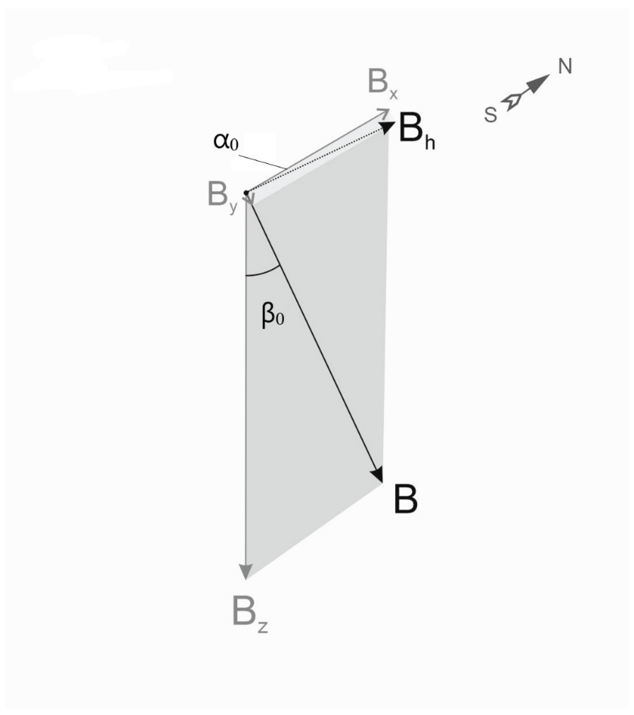
Figure 2.
Magnetic field characteristics under high-voltage power lines (PL). The length of the vector components is proportional to their magnetic induction. GMF direction indicated by north-south (NS) arrow corresponds to that of B. The vector of magnetic induction of the wire W right under PL has only a horizontal component oscillating between W1 and W2 (and W1 = W2). Lines of the wire’s MF encircling it in an annular manner are depicted as cylindric shapes, W is pointing tangentially to them. The total vector T = B + W periodically changes direction, oscillating between T1 and T2 (alternating current frequency is 50 Hz in Central Czechia). (a) An idealized example where a dog stands right under the wire that goes strictly parallel to the GMF direction (i.e. to the magnetic, not geographic, N-S axis). W is perpendicular to the horizontal vector Bh. The total field horizontal vector Th will oscillate between Th1 and Th2 (where Th1 = Th2) and have nonzero azimuth α1, α2 (the angles between B and Th, α2 = 360º - α1). The resulting inclination angles β1 = β2 will be slightly different from the GMF inclination I at the distance of over 300m from the wires. (b) In another idealized example the dog stands under the wire strictly perpendicular to the NS axis. Both W and Th are parallel to Bh (but Th1 ≠ Th2). The azimuth of Th1, Th2 is α1 = 0°, α2 = 180°. The inclination angles β1 ≠ β2 will significantly differ both from GMD inclination I and each other. (c) Schematic representation of the experiments in this study where a dog stands under the wire neither strictly parallel nor perpendicular to NS axis (like power lines parallel to topographic, not magnetic, N-S axis). Here, Th1 ≠ Th2, α1 ≠ α2 and β1 ≠ β2 ≠ I.
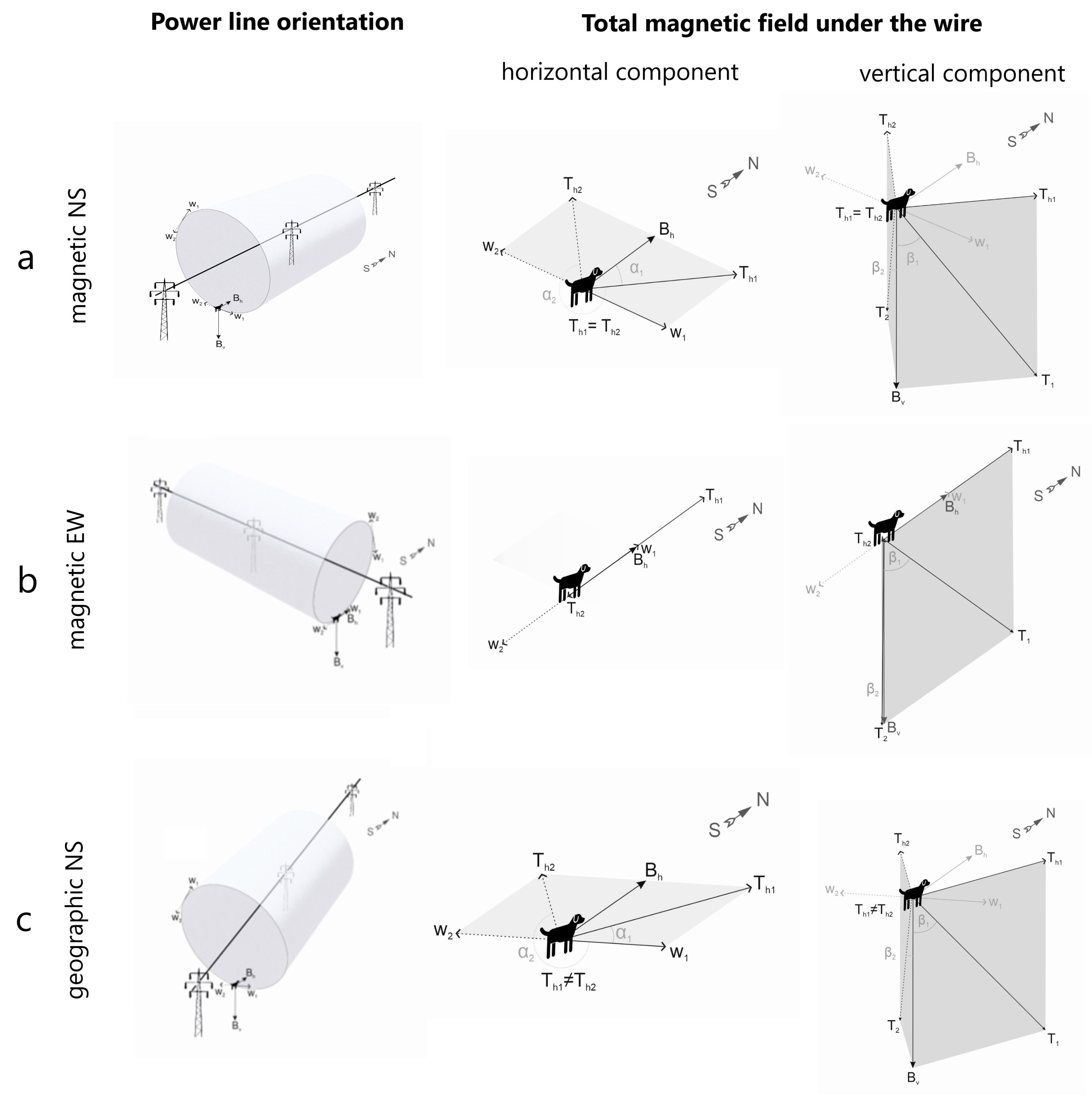
Figure 3.
Body orientation of the dogs during the measurements of the alignment. The bearings were recorded during dog's defecation or urination, measured as the azimuth of the axis going along thoracic spine (between scapulae) towards the head. Photo credits: J. Adamková.
Figure 3.
Body orientation of the dogs during the measurements of the alignment. The bearings were recorded during dog's defecation or urination, measured as the azimuth of the axis going along thoracic spine (between scapulae) towards the head. Photo credits: J. Adamková.

Figure 4.
Directional alignment of freely roaming dogs in control and experiment. (a) Representation of all datapoints, regardless of the magnetic weather. (b) Alignment during the periods of magnetic calm (RCD = 0%). (c) Alignment during the periods of moderate magnetic disturbance (RCD ≤ 2%). (d) Alignment during strong magnetic disturbances (RCD < 2%). The NS arrow represents the direction of GMF. The line with pillars represents the direction of PL wires. Two arrows represent the direction of total field horizontal components Th1, Th2. Rose diagram represents distribution of all bearings for all dogs. Smaller point diagram shows the distribution of means (one point – mean angle for one dog); the arrow represents the size and direction of Grand Mean (GM) vector r; N – total number of measurements for each condition.
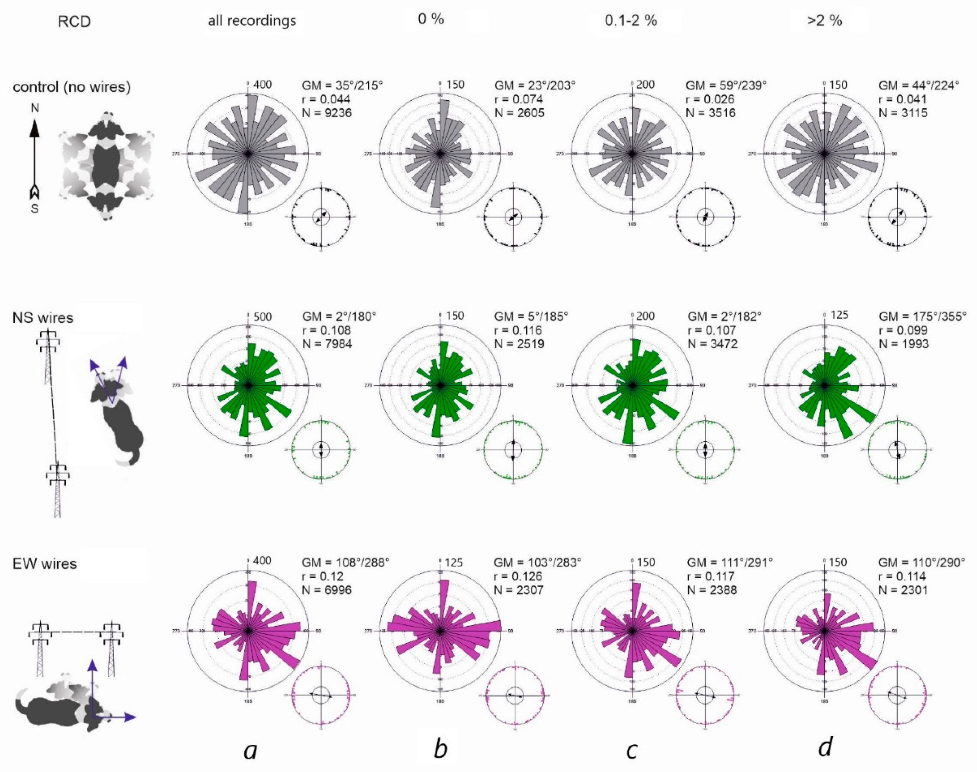
Figure 5.
Horizontal component of the total field T under the high-voltage PL versus dog’s alignment (2D representation of 3D system). N – geographical north, W – geographical west, figures on the scale indicate magnetic induction in µT. Bh – horizontal component of GMF at the given location away from the wires, Th1, Th2 – alternating horizontal component of the total field, dashed line represents median between Th1 and Th2.
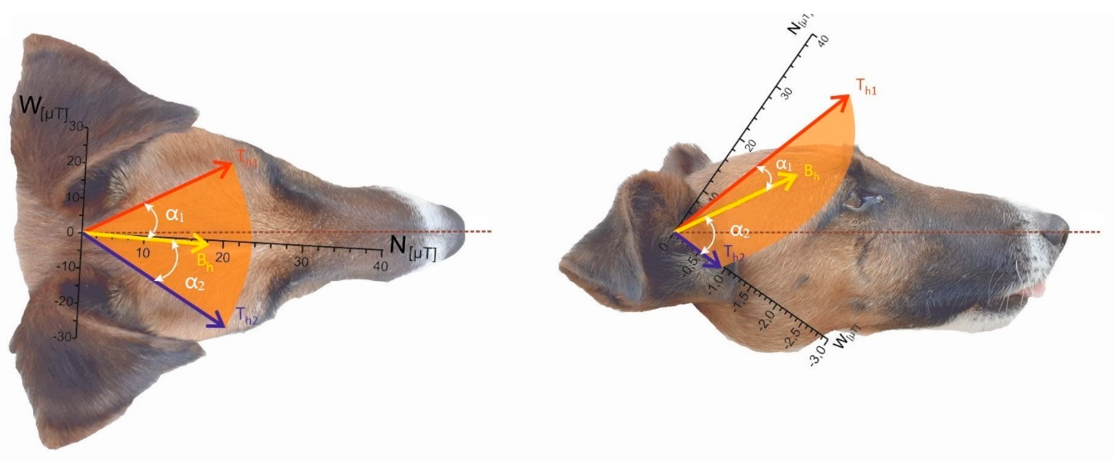

Table 1.
Characteristics of dogs’ alignment during magnetic calm and geomagnetic disturbances.
| Direction of the wires | Magnetic calm (RCD = 0%) | Moderate magnetic disturbances (RCD = 0.1-2%) | Strong magnetic disturbances (RCD > 2%) | ||||||
|---|---|---|---|---|---|---|---|---|---|
| Axial GM | r | k | Axial GM | r | k | Axial GM | r | k | |
| No wires | 23°/203° | 0.074 | 0.214 | 59°/239° | 0.026 | 0.086 | 44°/224° | 0.041 | 0.119 |
| Geographic NS | 5°/185° | 0.149 | 0.301 | 5°/185° | 0.113 | 0.228 | 2°/182° | 0.119 | 0.241 |
| Geographic EW | 103°/283° | 0.159 | 0.322 | 111°/291° | 0.101 | 0.203 | 110°/290° | 0.137 | 0.277 |
Table 2.
Magnetic field characteristics in the control (no high-voltage PL) and the experiments (NS- or EW-going PL). N – number of localities.
Table 2.
Magnetic field characteristics in the control (no high-voltage PL) and the experiments (NS- or EW-going PL). N – number of localities.
| Direction of the wires | N | Total field (T) characteristics | ||||||||
|---|---|---|---|---|---|---|---|---|---|---|
| Bx, µT | By, µT | Bz, µT | |T1|,µT | |T2|, µT | α1 | α2 | β1 | β2 | ||
| No wires | 26 | 19.98 ± 0.15 |
1.23 ± 0.14 | 44.62 ± 0.18 | |B| = 48.9 µT, Bh = 20.0 µT, D(α0) = 3.6°, I (β0) = 65.8° | |||||
| Geographic NS | 15 | 19.96 ± 0.13 | 1.23 ± 0.11 | 44.64 ± 0.15 | 52.4 | 53.3 | 41.5° | 311.5° | 42.8° | 58.4° |
| Geographic EW | 14 | 19.97 ± 0.14 | 1.19 ± 0.12 | 44.60 ± 0.17 | 59.9 | 44.6 | 91.0° | 358.3° | 48.1° | 88.5° |
Disclaimer/Publisher’s Note: The statements, opinions and data contained in all publications are solely those of the individual author(s) and contributor(s) and not of MDPI and/or the editor(s). MDPI and/or the editor(s) disclaim responsibility for any injury to people or property resulting from any ideas, methods, instructions or products referred to in the content. |
© 2025 by the authors. Licensee MDPI, Basel, Switzerland. This article is an open access article distributed under the terms and conditions of the Creative Commons Attribution (CC BY) license (https://creativecommons.org/licenses/by/4.0/).
Copyright: This open access article is published under a Creative Commons CC BY 4.0 license, which permit the free download, distribution, and reuse, provided that the author and preprint are cited in any reuse.


